Deep Autoencoder-based Z-Interference Channels with Perfect and Imperfect CSI

Abstract

A deep autoencoder (DAE)-based structure for end-to-end communication over the two-user Z-interference channel (ZIC) with finite-alphabet inputs is designed in this paper. The proposed structure jointly optimizes the two encoder/decoder pairs and generates interference-aware constellations that dynamically adapt their shape based on interference intensity to minimize the bit error rate (BER). An in-phase/quadrature-phase (I/Q) power allocation layer is introduced in the DAE to guarantee an average power constraint and enable the architecture to generate constellations with nonuniform shapes. This brings further gain compared to standard uniform constellations such as quadrature amplitude modulation. The proposed structure is then extended to work with imperfect channel state information (CSI). The CSI imperfection due to both the estimation and quantization errors are examined. The performance of the DAE-ZIC is compared with two baseline methods, i.e., standard and rotated constellations. The proposed structure significantly enhances the performance of the ZIC both for the perfect and imperfect CSI. Simulation results show that the improvement is achieved in all interference regimes (weak, moderate, and strong) and consistently increases with the signal-to-noise ratio (SNR). For instance, more than an order of magnitude BER reduction is obtained with respect to the most competitive conventional method at weak interference when $\rm SNR>15dB$ and two bits per symbol are transmitted. The improvements reach about two orders of magnitude when quantization error exists, indicating that the DAE-ZIC is more robust to the interference compared to the conventional methods.

I Introduction

Interference is a central issue in today’s multi-cell networks. The information-theoretic model for a multi-cell network is the interference channel (IC). There have been many efforts to find the capacity of the IC either with the same generality and accuracy used by Shannon for point-to-point systems [3, 4, 5, 6] or by seeking approximate solutions with a guaranteed gap to optimality at any signal-to-noise ratio (SNR) [7]. However, the capacity region of the two-user IC is only known for strong interference where decoding and canceling the interference is optimal [3]. Also, at very weak interference, sum-capacity is achievable by treating interference as noise [8, 9, 10], whereas, in general, decoding part of the interference and treating the remaining as noise is the best achievable scheme to date [5].

The aforementioned Shannon-theoretic works are based on Gaussian inputs. Despite being theoretically optimal, Gaussian alphabets are continuous and unbounded, and thus, are rarely applied in real-world communication. In practice, signals are generated using finite alphabet sets, such as phase-shift keying (PSK) and quadrature amplitude modulations (QAM). The performance gap between the finite alphabet input and the Gaussian input design is non-negligible [11]. However, conventional finite-alphabet approaches are based on predefined uniform constellations like QAM. These constellations are defined for point-to-point systems [12, 13, 14, 15] and their constellation shaping is oblivious to interference. Such an inability to respond to interference is an obstacle to improving the bit-error rate and spectral efficiency of today’s interference-limited communication systems.

In this paper, we consider the two-user single-input single-output (SISO) one-sided IC, also known as the Z-interference channel (ZIC). With Gaussian signaling, the capacity region of this channel is known only in the strong and very strong interference regimes [6]. However, Gaussian signaling is unsuitable for practical applications. Previous work has studied ZIC with finite alphabet sets in specific regimes and predefined uniform constellations. In [16], it is shown that rotating one input constellation (alphabet) can improve the sum-rate of the two-user IC in strong/very strong interference regimes. Later, an exhaustive search for finding the optimal rotation of the signal constellation was presented in [17]. In addition, a signaling design is proposed in [18] which applies a rotation to the channel which resembles rotating the input. The main focus of the above papers is to maximize the achievable rates, and they do not study bit-error rate (BER) performance. However, BER is a key metric and interference can severely reduce the BER by distorting the received constellation, when uniform constellations like QAM are employed.

Recent research has proved end-to-end learning as a promising approach for encoding, decoding, and signal representation to reduce BER [19]. Particularly, deep autoencoder (DAE) is a popular architecture for implementing end-to-end learning. It consists of an encoder that transforms input data into a low-dimensional representation to find its structure and a decoder that reconstructs the original input from this representation. DAE-based end-to-end communication is an emerging approach to finite-alphabet communication in which BER is the main performance measure and constellation design is inherent. DAE-based communication is introduces both for single- and multi-user systems by various groups [19, 20, 21, 22, 23, 24]. These studies indicate that the DAE surpasses current solutions and enhances performance beyond conventional methods [24].

Specifically, utilizing two DAEs for the transmitter/receiver pairs enables effective signal separation/decoding of original data even in the presence of interference, thereby paving the way for enhancing communication performance over the IC, as investigated in prior studies [19, 25, 26]. However, these studies have limitations as they focus solely on symmetric interference scenarios and compare their results against simple baselines like quadrature phase shift keying (QPSK), despite the fact that QPSK performs much worse than rotated QPSK in the context of the IC [16, 17, 18]. Further, the DAE designs in [19, 25, 26] produce symbols with fixed power levels and lack the ability to generalize to QAM-like constellations. Thus, they do not efficiently use the in-phase and quadrature-phase (I/Q) plane. Additionally, these designs assume perfect knowledge of channel state information (CSI), and the transition from perfect CSI to imperfect CSI remains unexplored.

I-A Motivation and Contribution

The above limitations has motivated us to investigate DAEs potential for the long-lasting problem of interference in more practical settings. We shed light on DAE-based communication over asymmetric interference with both perfect and imperfect CSI. Specifically, we design and train novel DAE-based architectures for the ZIC with finite-alphabet inputs. In the ZIC, two DAEs should be considered in two transmitter-receiver pairs. The two DAE pairs cooperate to avoid interference and adapt their constellation to the interference intensity. Our work is motivated by the following question: Can we design interference-aware constellations using DAEs? Will the gains remain/vanish if CSI is not perfect? We answer these questions by developing new structures and explaining how the designed nonuniform constellations lend themselves to interference mitigation in different regimes, and thus improving the BER.

The ZIC is characterized by local, short-range interference [27], where far-away users are not affected by interference. This simple channel model is a fundamental building block for more complex interference networks and its understanding is crucial in the field of interference research. As such, it has been widely studied in the literature of interference [6, 28, 29], as it provides insights into the limits interference-limited scenarios. By understanding the behavior of interference in the ZIC, we can develop more effective strategies to mitigate interference in more complex networks.

The main contributions of the paper are as follows:

• We design a DAE-based transmission structure for the ZIC and demonstrate its effectiveness across weak, moderate, and strong interference levels. We propose incorporating an average power constraint normalization layer that enables nonuniform constellations, resulting in more efficient utilization of the I/Q plane. The designed constellations are adaptive to the interference intensity, and morph in a way that the ‘receivers’ see distinguishable symbols, thereby improving BER even in the presences of interference. We also conduct a neural network ablation study to demonstrate the impact and necessity of each design element in our proposed model. This analysis provides valuable insights into the significance of each component and also serves to validate the overall architectural effectiveness.

• We extend the proposed structure to the finite-alphabet ZIC with imperfect CSI, where we consider both estimation and quantization errors. Particularly, CSI estimation errors pose confuses for DAE training and testing performance. Meanwhile, quantization errors, arising from limited feedback capacity, introduce undesirable rotations to the constellations. In order to develop a DAE that is robust against these errors, we introduce an equivalent system model that reduces the CSI parameters and ultimately lowers the BER.

• Our design directly accepts the transmission bits as its input rather than converting them to symbols and using one-hot vectors for the DAE input. This has two advantages. First, our design can directly minimize the BER and we do not need to worry about optimal bit-to-symbol mapping. Second, it reduces the complexity as to transmit $b$ bits, the input and output layers require only $b$ neurons whereas the one-hot vector method needs $2^{b}$ neurons.

It worth mentioning that, for benchmarking purposes, we use rotated uniform constellations, which have been proven to be more competitive than their unrotated counterparts. Our proposed DAE-ZIC shows significantly better BER performance for all interference regimes (weak, moderate, and strong interference). For perfect CSI, when averaged over SNRs from 0 to 20dB, 44% reduction in BER is achieved. At certain SNRs and interference regimes, the improvement is over an order of magnitude. For imperfect CSI, the overall reduction is about 40%. The gap between the DAE-ZIC and conventional methods is even larger when quantization error is applied.

I-B Organization

The remainder of this paper is organized as follows. We elaborate on the ZIC system model in Section II. The DAE design and the training approach are introduced in Section III. The system model with an imperfect CSI is derived in Section IV. The modifications for the DAE with an imperfect CSI is introduced in Section V. Numerical results are presented in Section VI, and the paper is concluded in Section VII.

Notation: $(\cdot)^{T}$ denotes transpose, $\mathbb{E}\{\cdot\}$ denotes expectation, and ${\rm{diag}}(\lambda_{1},\dots,\lambda_{n})$ represents the diagonal matrix with elements $\lambda_{1},\dots,\lambda_{n}$. $\mathcal{N}(\mu,\sigma^{2})$ and $\mathcal{CN}(\mu,\sigma^{2})$ are real and complex Gaussian distributions where $\mu$ and $\sigma^{2}$ are the mean and variance. $|\cdot|$ is the amplitude of a complex number.

II System Model of ZIC with Perfect CSI

Figure 1 shows the system model of a two-user complex SISO ZIC with perfect CSI. The two transmitter-receiver pairs wish to reliably transmit their messages while the transmission of the first pair interferes with the transmission of the second. The four nodes are named Tx1, Tx2, Rx1, and Rx2, as shown in Fig. 1. $h_{ij}$ refers to the channel gain from the $i$th transmitter to the $j$th receiver and $i,j\in\{1,2\}$. For ZIC, $h_{21}=0$. The received signals at the receivers can be written as

$$y_{1}=h_{11}x_{1}+h_{21}x_{2}+n_{1},$$ (1a)

$$y_{2}=h_{22}x_{2}+n_{2},$$ (1b)

in which $x_{1}$ and $x_{2}$ denote the transmitted symbols of Tx1 and Tx2. The transmitted signals are complex-valued with finite-alphabets and variances $\mathbb{E}\{|x_{1}|^{2}\}=P_{1}$ and $\mathbb{E}\{|x_{2}|^{2}\}=P_{2}$ in which $P_{1}$ and $P_{2}$ are the power budgets of the two transmitters. The channel coefficients are complex random variables

$$h_{ij}\triangleq r_{ij}e^{j\theta_{ij}}\sim\mathcal{CN}(\mu_{h},\sigma_{h}^{2}),$$ (2)

where $\mu_{h}$ and $\sigma_{h}^{2}$ are the mean and variance of the channel distribution, and $r_{ij}$ and $\theta_{ij}$ represent the magnitude and phase of $h_{ij}$. Also, $n_{1}$ and $n_{2}$ are the complex-valued independent and identically distributed (i.i.d.) additive white Gaussian noise with zero means and variances $\sigma_{1}^{2}$ and $\sigma_{2}^{2}$. Without loss of generality, we assume the noise powers at the two receivers’ sides are the same, i.e., $\sigma_{1}^{2}=\sigma_{2}^{2}=\sigma^{2}$ [28].

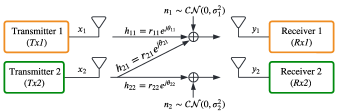
Figure 1: System model of the ZIC.

II-A The Equivalent System Model of the ZIC

It is known that, without loss of generality, the channel gains of the direct transmission links can be modeled as one, shown in Fig. 2(b), [29, 30, 28]. The interference gain is also real-valued for both real- and complex-valued systems. When CSI is available and if we apply pre- and post-processing illustrated in Fig. 2(a), such a system model in Fig. 1 is equivalent to that of Fig. 2(b). The Tx2 applies $e^{j(\theta_{11}-\theta_{21})}$ to cancel the phase of $h_{21}$ and align its phase with that of $h_{11}$. The Rx1 and Rx2 applies $h_{11}^{-1}$ and $h_{22}^{-1}e^{j(\theta_{21}-\theta_{11})}$ to normalize the channel gain to one. Then, the received post-processed signals are

$$\bar{y}_{1}=h_{11}^{-1}y_{1}=x_{1}+r_{21}r_{11}^{-1}x_{2}+n_{1}h_{11}^{-1},$$ (3a)

$$\bar{y}_{2}=h_{22}^{-1}e^{j\theta_{21}}y_{2}=x_{2}+e^{j\theta_{21}}{n_{1}}h_{22}^{-1}.$$ (3b)

By defining

$$\sqrt{\alpha}\triangleq r_{21}r_{11}^{-1},$$ (4a)

$$\bar{n}_{1}\triangleq n_{1}h_{11}^{-1},\;\textmd{and},\;\bar{n}_{2}\triangleq e^{j\theta_{21}}{n_{1}}h_{22}^{-1},$$ (4b)

we have the system model in Fig. 2(b) as

$$\bar{y}_{1}=\bar{h}_{11}x_{1}+\sqrt{\alpha}x_{2}+\bar{n}_{1},$$ (5a)

$$\bar{y}_{2}=\bar{h}_{22}x_{2}+\bar{n}_{2}.$$ (5b)

where $\bar{h}_{11}=\bar{h}_{22}=1$ and $\bar{h}_{21}=\sqrt{\alpha}$ are the equivalent channel gains.

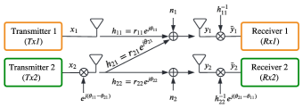
(a) Original system model

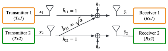
(b) Equivalent system model

Figure 2: The equivalent system model of the ZIC.

Thus, the two system models in Fig. 1 and Fig. 2 are equivalent. Hence, we follow the existing studies and use the system model in Fig. 2(b), and consider a fixed $\sqrt{\alpha}$ at each time. It is worth mentioning that both actual channel gains and noise ($h_{ij}$ and $n_{i}$, $i,j\in\{1,2\}$) are Gaussian. In this paper, we assume a slow fading scenario with

$$\bar{n}_{i}\sim\mathcal{CN}(0,\sigma_{i}^{2}r_{ii}^{-2}).$$ (6)

III Deep Autoencoder with Perfect CSI

Existing studies [16, 17, 31] use standard QAM constellations at each transmitter. Such constellations are fixed and are not adjustable according to the interference intensity. To further improve the transmission performance, we propose a DAE-based transmission for the two-user ZIC, named DAE-ZIC. The architecture is shown in Fig. 3.

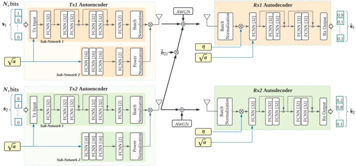
Figure 3: The architecture of the two-user DAE-ZIC implemented by two pairs of deep autoencoders. Each transmitter of the ZIC contains two sub-networks. Sub-network 1 mainly generates the constellation and sub-network 2 is used to implement the average power constraint. The receivers decode their bits from the received signal. This architecture is based on the system model in Fig. 2(b). $\eta$ is a power control parameter defined in (15).

III-A The Architecture of DAE-ZIC

The DAE-ZIC consists of two pairs of DAEs. Each pair performs an end-to-end transmission, which includes input bits, autoencoder at the transmitter, channel and noise layers, autoencoder at the receiver, and final output bits.

III-A1 Network Input

Each transmitter sends $N_{s}$ bits to the corresponding receiver. The interference channel coefficient $\sqrt{\alpha}$ is known at the transmitter and receiver and is appended to the input bit vector. Then, both the transmitters and receivers have the knowledge of the CSI. The two transmitters are expected to jointly design their constellations and the receivers will decode correspondingly.

III-A2 Transmitter DAE

As shown in Fig. 3, the DAE of the transmitter contains two sub-networks: Sub-network 1 and Sub-network 2. Sub-network 1 converts the input bit-vector to symbols with unit power in the I/Q components. Sub-network 2 performs power allocation, which controls the power of the I/Q components. The two sub-networks combines in parallel to yield a nonuniform constellation. The batch normalization in sub-network 1 together with sub-network 2 realize the average power constraint at the transmit antenna. Having an average power constraint is necessary especially for SISO systems. In this way, the I/Q plane is used efficiently, like QAM. Otherwise, the DAE can only produce constant-power constellations, like PSK, where constellation points are on a circle which is not efficient in terms of BER.

The components of sub-network 1 are fully connected layers (FCNN), residual connections, or shortcuts, to alleviate the vanishing gradient effect, and the output batch normalization layer. The activation function of the FCNN layers is tanh, except for the last layer which has two hidden nodes and no activation function.

Let the batch size be $N_{B}$. The output of the last FCNN is

$$\mathbf{X}_{\textmd{fcnn}}\triangleq[\mathbf{x}_{\textmd{fcnn}}^{\textmd{I}},\;\mathbf{x}_{\textmd{fcnn}}^{\textmd{Q}}],$$ (7)

where $\mathbf{x}_{\textmd{fcnn}}^{\textmd{I}}$ and $\mathbf{x}_{\textmd{fcnn}}^{\textmd{Q}}\in\mathbb{R}^{N_{B}\times 1}$ are the outputs of the two hidden nodes and represent I/Q of the complex-valued signal. Since the FCNN has unbounded outputs, it cannot guarantee a power constraint at the transmitter. We propose the transmitter design shown in Fig. 3 to achieve an average power constraint at each antenna. First, we use batch normalization in sub-network 1 to unify the average power of I/Q independently. The batch normalization layer linearly normalizes ${\mathbf{x}}_{\textmd{fcnn}}^{\textmd{I}}$ and ${\mathbf{x}}_{\textmd{fcnn}}^{\textmd{Q}}$, in which the normalized vectors $\mathbf{x}_{B}^{\textmd{I}}$ and $\mathbf{x}_{B}^{\textmd{Q}}$ are given by

$$\mathbf{x}_{B}^{\textmd{I}}\triangleq\beta^{\textmd{I}}\cdot{\mathbf{x}}_{\textmd{fcnn}}^{\textmd{I}},\;\;\mathbf{x}_{B}^{\textmd{Q}}\triangleq\beta^{\textmd{Q}}\cdot{\mathbf{x}}_{\textmd{fcnn}}^{\textmd{Q}},$$ (8)

where $\bm{\beta}\triangleq[\beta^{\textmd{I}},\;\beta^{\textmd{Q}}]^{T}$ contains two factors for normalization.

In sub-network 2, the power allocation of the I/Q components is determined by the FCNN layers, which take the input value $\sqrt{\alpha}$ into account. The FCNN layers calculates the powers of I/Q components, and the power normalization block limits the total power to $P_{t}$, thus achieving the intended power control. The powers of $\mathbf{x}_{B}^{\textmd{I}}$ and $\mathbf{x}_{B}^{\textmd{Q}}$ (i.e., each batch of I/Q signals) are multiplied by $\gamma^{\textmd{I}}$ and $\gamma^{\textmd{Q}}$, which are the outputs of Sub-network 2. Defining the input and output of the power normalization layer as ${\bm{\gamma}}_{0}\triangleq[\gamma^{\textmd{I}}_{0},\;\gamma^{\textmd{Q}}_{0}]^{T}\in\mathbb{R}^{2\times 1}$ and ${\bm{\gamma}}\triangleq[\gamma^{\textmd{I}},\;\gamma^{\textmd{Q}}]^{T}\in\mathbb{R}^{2\times 1}$ respectively, the power normalization layer normalizes its input and scales its power, i.e., ${\bm{\gamma}}=\sqrt{P_{t}}\frac{{\bm{\gamma}}_{0}}{|{\bm{\gamma}}_{0}|}$. Thus, ${\bm{\gamma}}^{T}{\bm{\gamma}}=P_{t}$. Such an operation can be done via the Lambda layer in Keras [32]. Finally, the outputs of the batch normalization and power normalization are multiplied together, i.e.,

$$\mathbf{x}_{\textmd{out}}^{\textmd{I}}\triangleq\gamma^{\textmd{I}}\cdot\mathbf{x}_{B}^{\textmd{I}},\;\;\mathbf{x}_{\textmd{out}}^{\textmd{Q}}\triangleq\gamma^{\textmd{Q}}\cdot\mathbf{x}_{B}^{\textmd{Q}}.$$ (9)

The powers of $\mathbf{x}_{\textmd{out}}^{\textmd{I}}$ and $\mathbf{x}_{\textmd{out}}^{\textmd{Q}}$ are $\gamma^{\textmd{I}}$ and $\gamma^{\textmd{Q}}$, respectively. In short, batch normalization is applied to I and Q components separately and along the time axis (batch by batch) while power normalization scales the power of I/Q components at each time to reach the average power constraint. That is, the two normalization operations are implemented in different dimensions. The final output of the transmitter is

$$\mathbf{X} \triangleq[\mathbf{x}_{\textmd{out}}^{\textmd{I}},\;\mathbf{x}_{\textmd{out}}^{\textmd{Q}}]$$

$$=[\mathbf{x}_{B}^{\textmd{I}},\;\mathbf{x}_{B}^{\textmd{Q}}]\cdot\textmd{diag}({\bm{\gamma}})$$

$$=[\mathbf{x}_{\textmd{fcnn}}^{\textmd{I}},\;\mathbf{x}_{\textmd{fcnn}}^{\textmd{Q}}]\cdot\textmd{diag}({\bm{\beta}})\cdot\textmd{diag}({\bm{\gamma}}).$$ (10)

where $\mathbf{x}_{\textmd{fcnn}}^{\textmd{I}}$ and $\mathbf{x}_{\textmd{fcnn}}^{\textmd{Q}}$ are the output of the FCNN layer in sub-network 1 and represent the preliminary I/Q signals, $\bm{\beta}$ normalizes the power of each batch, and $\bm{\gamma}$ controls the power of the I/Q signals such that average power is $P_{t}$.

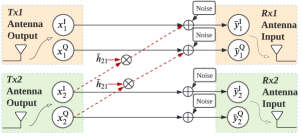
Figure 4: Form a SISO complex-valued channel by a 2x2 MIMO real-valued channel.

III-A3 Channel Implementation

The channel is formed following (1). The complex-valued SISO channel is achieved by real values intuitively shown in Fig. 4. At Rx1, the received signal is $\bar{y}_{1}=\bar{y}_{1}^{\textmd{I}}+j\bar{y}_{1}^{\textmd{Q}}$,

$$\left[\begin{matrix}\bar{y}_{1}^{\textmd{I}}\\ \bar{y}_{1}^{\textmd{Q}}\end{matrix}\right]=\left[\begin{matrix}x_{1}^{\textmd{I}}\\ x_{1}^{\textmd{Q}}\end{matrix}\right]+\bar{h}_{21}\cdot\left[\begin{matrix}x_{2}^{\textmd{I}}\\ x_{2}^{\textmd{Q}}\end{matrix}\right]+\left[\begin{matrix}\bar{n}_{1}^{\textmd{I}}\\ \bar{n}_{1}^{\textmd{Q}}\end{matrix}\right],$$ (11)

where $\bar{y}_{1}^{\textmd{I}}$ and $\bar{y}_{1}^{\textmd{Q}}$ are the I/Q components of the received signal, $x_{i}^{\textmd{I}}$ and $x_{i}^{\textmd{Q}}$ are the I/Q components of the $i$the transmitter, and $\bar{n}_{i}^{\textmd{I}},\bar{n}_{i}^{\textmd{Q}}\sim\mathcal{N}(0,\frac{1}{2}\sigma_{N}^{2}r_{ii}^{-2})$ are the I/Q components of the complex-valued. Similarly, the received signal for Rx2 is $\bar{y}_{2}=\bar{y}_{2}^{\textmd{I}}+j\bar{y}_{2}^{\textmd{Q}}$,

$$\left[\begin{matrix}\bar{y}_{2}^{\textmd{I}}\\ \bar{y}_{2}^{\textmd{Q}}\end{matrix}\right]=\left[\begin{matrix}x_{2}^{\textmd{I}}\\ x_{2}^{\textmd{Q}}\end{matrix}\right]+\left[\begin{matrix}\bar{n}_{2}^{\textmd{I}}\\ \bar{n}_{2}^{\textmd{Q}}\end{matrix}\right].$$ (12)

The additive Gaussian white noise (AWGN) is implemented by a Gaussian noise layer in Keras. The noise power is set according to SNR in the training and testing stages.

III-A4 Receiver DAE

The received signals are $\bar{y}_{1}$ and $\bar{y}_{2}$. To ensure the receiver networks have a finite input range, we use batch normalization layers in Keras unifying the power of the received signals, i.e.,

$${y}_{\textmd{B},i}=\xi\cdot\bar{y}_{i},\;\;E\{|{y}_{\textmd{B},i}|^{2}\}=1,\;\;\forall i\in\{1,2\},$$ (13)

where $\xi$ is a coefficient to reach the unit power. The process details and settings are the same as those in the transmitter.

We further define the desired signal for Rx1 as

$$x_{\textmd{D},1}\triangleq x_{1}+\sqrt{\alpha}x_{2}.$$ (14)

$x_{\textmd{D},1}$ contains the true desired signal $x_{1}$ and the interference $\sqrt{\alpha}x_{2}$. The goal of the receiver is to decode $x_{1}$ for an arbitrary $x_{2}$ in its constellation. The desired signal of Rx2 is $x_{\textmd{D},2}\triangleq x_{2}$. However, the normalization of the received signal (13) causes the power of the desired signal to vary with the SNR. Hence, the autoencoder should adjust the decoding boundary according to the SNR, which is an extra burden. So, we turn to normalize the desired signal using linear factor, $\eta$, multiplied on the batch normalization output, i.e.,

$$y_{\textmd{D},i}=\eta\cdot{y}_{\textmd{B},i},\;\eta\triangleq\sqrt{1+\frac{P_{\textmd{D,i}}}{\sigma_{N}^{2}}},\quad\forall i\in\{1,2\},$$ (15)

where $P_{\textmd{D},i}$ is the power of the desired signal $x_{\textmd{D},i}$ and $\sigma_{N}^{2}$ is the noise power. The batch normalization normalizes the desired signals using pre-processing $\eta$. Then, the normalized signal, $y_{\textmd{D},i}$, together with the feature of the ZIC, $h_{21}=\sqrt{\alpha}$, are sent to the rest of the FCNN layers. The final output of the DAE is an estimation of the transmitted bit-vectors, $\hat{\mathbf{s}}_{1}$ and $\hat{\mathbf{s}}_{2}$, as shown in Fig. 3.

The activation function of the output layer is sigmoid function, i.e., $f(s)=\frac{1}{1+e^{-s}}$. Thus, assuming the input of the final layer, marked as Rx Output in Fig. 3, of $i$th receiver is $\mathbf{y}_{F,i}$, the output equations can be written as $\hat{\mathbf{s}}_{i}=f(\mathbf{y}_{F,i})$. The sigmoid function is commonly used because it outputs a value between 0 and 1, which can be interpreted as a probability of the input belonging to the positive class. This function is also differentiable, which is important for backpropagation during training of neural networks.

III-A5 Loss Function

In our DAE-ZIC, each receiver has its own estimation of the transmitted bits. Then, the overall loss function of the DAE-ZIC is $\mathcal{L}=\mathcal{L}_{1}+\mathcal{L}_{2}$, where $\mathcal{L}_{1}$ and $\mathcal{L}_{2}$ are the loss at Rx1 and Rx2. Each output vector in the two receivers represents binary messages, then the network can be trained using binary cross-entropy loss:

$$\mathcal{L}_{i}=\frac{1}{N_{B}}\sum_{n=1}^{N_{B}}(\mathbf{s}_{i,n})^{T}\log\hat{\mathbf{s}}_{i,n}+(1-\mathbf{s}_{i,n})^{T}\log(1-\hat{\mathbf{s}}_{i,n}),$$ (16)

where $i\in\{1,2\}$ distinguishes the users, $N_{B}$ is the batch size, $\mathbf{s}_{i,n}$ is the $n$th input bit-vector in the batch, and $\hat{\mathbf{s}}_{i,n}$ is the corresponding output. The loss function treats each element of the DAE output as a 0/1 classification task. The binary cross-entropy loss function is commonly used for multi-label classification problems, where each example can have multiple binary labels. The loss function measures the difference between the predicted probability of each label being present in the example and the true probability of the label being present. Finally, the loss is the summation of the loss of $N_{s}$ tasks, where $N_{s}$ is the number of bits in the transmission. In the training process, the backpropagation algorithm passes $\mathcal{L}_{1}$ to Rx1 and it will further go to Tx1 and Tx2, whereas $\mathcal{L}_{2}$ affects Rx2 and Tx2.

III-B Training Procedure of the DAE-ZIC

Due to the difficulty of training a single network across all values of the interference gain $\alpha$, distinct instances of DAEs are employed for a few different ranges of $\alpha$. For each training session, a value for $N_{s}$ is selected and the desired range for $\alpha\in[\alpha_{\min},\alpha_{\max}]$ is specified. During the training process, all four sub-networks are trained simultaneously. The DAE is trained iteratively using random values of $\alpha$ within this interval. For each $\alpha$, the DAE undergoes training for $E_{p}$ epochs with a mini-batch size of $N_{B}$ and a constant learning rate of $l_{r}$. After training the DAE for $N_{d}$ different values of $\alpha$, the learning rate is reduced to $d_{r}l_{r}$. A comprehensive description of the training procedure, including the simultaneous training of all sub-networks to adapt to the ZIC interference patterns, can be found in Algorithm 1.

Algorithm 1 Training Procedure for the DAE-ZIC

1:Fix $N_{s}$, $\alpha_{\min}$, and $\alpha_{\max}$.

2:Set $P_{t}=1$W and SNR$=10$dB.

3:Set $N_{\alpha}=30,000$, the number of channels.

4:Set $E_{p}=10$, the number of the epochs.

5:Set $N_{B}=10^{4}$, the batch size.

6:Set $l_{r}=10^{-2}$, the initial learning rate, which will drop to $d_{r}l_{r}=0.95l_{r}$ after every $N_{d}=200$ trained channels.

7:Initialize the DAE-ZIC network.

8:for index $i_{\alpha}$ from $1$ to $N_{\alpha}$ do

9:     Uniformly and randomly select one $\alpha\in[\alpha_{\min},\alpha_{\max}]$.

10:     Randomly generate $h_{11}$ and $h_{22}$ using (2).

11:     Normalize the channel using (5).

12:     Update $\bar{h}_{21}=\sqrt{\alpha}$ in the DAE-ZIC in (11).

13:     Set the variance of the noise layer according to (6).

14:     for index $i_{e}$ from $1$ to $E_{p}$ do

15:         Randomly generate $N_{B}$ bit vectors.

16:         Update the weights of the DAE-ZIC using Adam.

17:     end for

18:     Set learning rate $l_{r}=d_{r}l_{r}$ if $i_{\alpha}/N_{d}$ is an integer.

19:end for

IV System Model with Imperfect CSI

In this section, we consider the ZIC with imperfect CSI and find its equivalent channel. The CSI imperfectness comes from two sources: the error in the estimation of the CSI at each receiver and the error due to the quantization of the CSI before feeding it back to the transmitter. The system model is depicted in Fig. 5(a), in which both the estimation error and quantization error are considered. In general, the notation is similar to Section II-A. One main difference is that the estimation errors $\varepsilon_{ij}$ occur at the receivers when we estimate the channel coefficients $\hat{h}_{ij}$. The imperfectness of $\hat{h}_{ij}$ affects the decoding process. Besides, the quantization error occurs when the parameters need to be fed back to another node. For example, the Tx2 applies

$$\theta_{q}\triangleq Q(\hat{\theta}_{11}-\hat{\theta}_{21}),$$ (17)

to cancel the phase of $h_{21}$ where $\theta_{11}$ and $\hat{\theta}_{21}$ are estimated by Rx1 and $Q(\cdot)$ is a quantization function. Ideally, $\theta_{q}$ is expected to be $\hat{\theta}_{11}-\hat{\theta}_{21}$, however, the quantization error exists which is defined as

$$\theta_{\delta}\triangleq\theta_{q}-(\hat{\theta}_{11}-\hat{\theta}_{21}),$$ (18)

The quantization error is included in $\bar{h}_{21}$ in Fig. 5(b). The details of the system model and the two types of errors are given as follows.

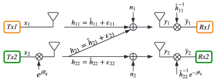
(a) Original system model with imperfect CSI. The angle $\theta_{q}$ is the pre-processing angle defined in (17).

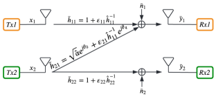
(b) Equivalent system model with imperfect CSI. The angle $\theta_{\delta}$ is the quantization error defined in (18).

Figure 5: System model of the ZIC with imperfect CSI.

IV-1 Estimation Error

The estimated channel gain is modeled as in [33]

$$\hat{h}_{ij}\triangleq\hat{r}_{ij}e^{j\hat{\theta}_{ij}}={h}_{ij}-\varepsilon_{ij},$$ (19)

where

$$h_{ij}\sim\mathcal{CN}(\mu_{h},\sigma_{h}^{2})$$ (20)

is the actual channel with mean $\mu_{h}$ and variance $\sigma_{h}^{2}$, and

$$\varepsilon_{ij}\sim\mathcal{CN}(0,\sigma_{E}^{2})$$ (21)

is the estimation error in which $\sigma_{E}^{2}$ is the variance of the error, and $ij\in\{11,21,22\}$. $\hat{h}_{11}$ and $\hat{h}_{21}$ are estimated by Rx1 while $\hat{h}_{22}$ is estimated by Rx2. The estimated channel coefficients are determined by the actual channel and noise, hence, $\hat{h}_{ij}\sim\mathcal{CN}(\mu_{h},\sigma_{h}^{2}+\sigma_{E}^{2})$. Once the actual channel and noise are determined, we have $h_{ij}=\hat{h}_{ij}+\varepsilon_{ij}$ as the channels in Fig. 5(a).

Tx2 keeps the pre-processing based on a feedback angle, $\theta_{q}$. Rx1 applies post-processing in Fig. 2 based on the $\hat{h}_{ij}$. Then, $\bar{y}_{i}$ in (3a) becomes

$$\bar{y}_{1}= \left(1+\frac{\varepsilon_{11}}{\hat{h}_{11}}\right)x_{1}+\frac{n_{1}}{\hat{h}_{11}}+e^{j\theta_{q}}\left(\frac{\hat{h}_{21}}{\hat{h}_{11}}+\frac{\varepsilon_{21}}{\hat{h}_{11}}\right)x_{2},$$ (22a)

$$\bar{y}_{2}= \left(1+\frac{\varepsilon_{22}}{\hat{h}_{22}}\right)x_{2}+\frac{n_{2}}{\hat{h}_{22}},$$ (22b)

which can be rewritten as

$$\bar{y}_{1}= \bar{h}_{11}x_{1}+\bar{h}_{21}x_{2}+\bar{n}_{1},$$ (23a)

$$\bar{y}_{2}= \bar{h}_{22}x_{2}+\bar{n}_{2},$$ (23b)

by defining

$$\bar{h}_{ii}\triangleq(1+\varepsilon_{ii}\hat{h}_{ii}^{-1}),$$ (24a)

$$\bar{h}_{21}\triangleq(\hat{r}_{21}\hat{r}_{11}^{-1}e^{j\theta_{\delta}}+\varepsilon_{21}\hat{h}_{11}^{-1}),$$ (24b)

$$\bar{n}_{i}\triangleq n_{i}\hat{h}_{ii}^{-1}\sim\mathcal{CN}(0,\sigma_{N}^{2}\hat{r}_{ii}^{-2}).$$ (24c)

In (24b), $\theta_{\delta}$ is the residual angle caused by the quantized feedback, which is defined in (18) where ${\theta}_{q}$ is the feedback angle as (25b).

IV-2 Quantization Error

Next, the transmitters require the knowledge of CSI to perform pre-processing and modification on constellation for enhanced performance. However, due to the limited feedback resources, the feedback information is quantized. This generates another source of imperfection. The estimated and quantized parameters owned by each end are shown in Fig. 6. Rx1 has the estimated $r_{11}$, $r_{21}$, $\theta_{11}$, and $\theta_{21}$. Rx2 has the estimated $r_{22}$, and $\theta_{22}$. To make all the four nodes access to the channel knowledge, both

$$\alpha_{q}=Q(\hat{\alpha})=Q({\hat{r}_{21}^{2}}\cdot{\hat{r}_{11}^{-2}}),$$ (25a)

$$\color[rgb]{0,0,0}\theta_{q}=Q(\hat{\theta})=Q(\hat{\theta}_{11}-\hat{\theta}_{21})=\hat{\theta}_{11}-\hat{\theta}_{21}+\theta_{\delta},$$ (25b)

are sent to the transmitter and Rx2, where $Q(\cdot)$ is a uniform quantizer with accuracy $N_{q}$, $\hat{\alpha}$ is the estimation of the interference intensity, $\hat{\theta}=\hat{\theta}_{11}-\hat{\theta}_{21}$, and $\theta_{\delta}$ is the same quantization error in (18). The quantizer $Q(\cdot)$ uniformly divides the region of the input variable into $2^{N_{q}}$ segments. The region for $\alpha$ and angle are $[0,3]$ and $[-\pi,\pi]$, respectively. The middle value of the segment is the quantization result if the input value of $Q(\cdot)$ is within this segment.

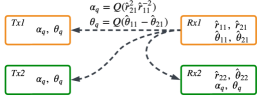
Figure 6: Feedback process for the ZIC transmission. $\alpha_{q}$ and $\theta_{q}$ are the only feedback parameters.

IV-3 Implementation of the imperfect ZIC

To implement the imperfect channel model, we randomly generate actual channels $h_{11}$ and $h_{22}$ and estimation errors $\varepsilon_{11}$, $\varepsilon_{22},$ and $\varepsilon_{21}$. Then, $\hat{h}_{11}$ and $\hat{h}_{22}$ are determined by (19). We give interference gain $\alpha$ and then $h_{21}=\sqrt{\alpha}e^{i\theta_{21}}$, where $\theta_{21}$ is a random uniformly distributed angle on $[0,2\pi)$. After actual channels are generated, the receivers will have the estimated CSI and can normalize the channel as Fig. 5(b). The receivers will then assume the channel gains are unity and the Rx1 assumes the interference gain is ${\hat{\alpha}}=|\hat{r}_{21}\hat{r}_{11}^{-1}|^{2}$.

It is worth mentioning that, $\bar{y}_{1}$ or $\bar{y}_{2}$ will go to infinity when the estimated channel gains ($r_{11}$ or $r_{22}$) are close to zero. In this case, the transmission is not reliable due to the wrong information obtained from the channel estimation no matter if the equalization in (23a) is applied or not. The receivers will suffer from a mismatch between the received symbol and the constellation. In the channel generation for the imperfect model, we keep the channel only if

$$\max(\left|\frac{\varepsilon_{11}}{\hat{h}_{11}}\right|,\left|\frac{\varepsilon_{22}}{\hat{h}_{22}}\right|,\left|\frac{\varepsilon_{21}}{\hat{h}_{11}}\right|)<T.$$ (26)

where $T$ is a threshold. We use $T=1$ in this paper so that the estimation errors is not dominating in $\bar{h}_{ii}$ in (24a).

To summarize, for $i,j\in\{1,2\}$,

• The actual channels coefficients are $h_{ij}$ in (20).

• The estimated channels coefficients are $\hat{h}_{ij}$, as in (19);

• After the equalization, the equivalent channel coefficients are $\bar{h}_{ij}$, as in (24a)-(24b);

• After normalization, Rx1 and Rx2 will assume the direct channel gains are one and the interference gain is $\hat{\alpha}$.

• Rx1 knows both the estimated and quantized parameters. Rx1 sends feedback parameters ($\hat{\alpha}_{q}$ and $\hat{\theta}_{q}$) to Tx1, Tx2, and Rx2.

Remark 1

If $\sigma_{E}^{2}=0$ and $N_{q}\to\infty$ (i.e., the CSI is perfect), the system in Fig. 5(b) reduces to that of Fig. 2(b).

V Deep Autoencoder for ZIC with Imperfect CSI

The channel implementation should follow the imperfect ZIC model in Section IV. The equivalent channels, $\bar{h}_{ij}$s, are set into the channel layers inside the DAE-ZIC. Different from the perfect channel case in (11)-(12) and Fig. 4, the I/Q components become

$$\left[\begin{matrix}\bar{y}_{1}^{\textmd{I}}\\ \bar{y}_{1}^{\textmd{Q}}\end{matrix}\right]=\bar{\mathbf{H}}_{11}\left[\begin{matrix}x_{1}^{\textmd{I}}\\ x_{1}^{\textmd{Q}}\end{matrix}\right]+\bar{\mathbf{H}}_{21}\left[\begin{matrix}x_{2}^{\textmd{I}}\\ x_{2}^{\textmd{Q}}\end{matrix}\right]+\left[\begin{matrix}\bar{n}_{1}^{\textmd{I}}\\ \bar{n}_{1}^{\textmd{Q}}\end{matrix}\right],$$ (27a)

$$\left[\begin{matrix}\bar{y}_{2}^{\textmd{I}}\\ \bar{y}_{2}^{\textmd{Q}}\end{matrix}\right]=\bar{\mathbf{H}}_{22}\left[\begin{matrix}x_{2}^{\textmd{I}}\\ x_{2}^{\textmd{Q}}\end{matrix}\right]+\left[\begin{matrix}\bar{n}_{2}^{\textmd{I}}\\ \bar{n}_{2}^{\textmd{Q}}\end{matrix}\right],$$ (27b)

in which $x_{i}^{\textmd{I}}$ and $x_{i}^{\textmd{Q}}$ are I/Q components of the transmitted signals, where $i\in\{1,2\}$ denotes the users; similarly, $\bar{y}_{i}^{\textmd{I}}$ and $\bar{y}_{i}^{\textmd{Q}}$ are I/Q components of the received signals; and, $\bar{n}_{i}^{\textmd{I}}$ and $\bar{n}_{i}^{\textmd{Q}}$ are the noises. $\bar{\mathbf{H}}_{ij}$ is the real form of the complex-valued channel $\bar{h}_{ij}$ in (24a)-(24b),

$$\bar{\mathbf{H}}_{ij}=\left[\begin{matrix}\bar{h}_{ij}^{\textmd{I}}&-\bar{h}_{ij}^{\textmd{Q}}\\ \bar{h}_{ij}^{\textmd{Q}}&\quad\bar{h}_{ij}^{\textmd{I}}\end{matrix}\right].$$ (28)

where $\bar{h}_{ij}=\bar{h}_{ij}^{\textmd{I}}+j\bar{h}_{ij}^{\textmd{Q}}$. Therefore, we add an FCNN layer to implement each of the channels. The weight of the channel layer is $\bar{\mathbf{H}}_{ij}$ in (28). These channel layers have zero bias, no activation function, and are non-trainable. The weight will be replaced only if the channel is updated during the training and testing.

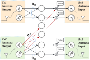
Figure 7: Implementation of the channels inside the proposed DAE network.

In contrast to the scenario with perfect CSI, illustrated in Fig. 3, the presence of imperfections in the CSI introduces distinct considerations to our approach.

• Differences in parameters. In the case of imperfect CSI, the parameter $\alpha$ is not directly available for utilization. The imperfectness at Rx1 side comes from the estimation of the interference gain $\hat{\alpha}$ and angle $\hat{\theta}$. Rx1 transmits $\alpha_{q}$ and $\theta_{q}$ (quantized values of $\hat{\alpha}$ and $\hat{\theta}$) to Tx1, Tx2, and Rx2, as shown in Fig. 6. Thus, the information in three nodes suffer from both sources of imperfectness, i.e., estimation and quantization errors.

• Differences in network input configurations. For Rx1, the input comprises the non-quantized $\sqrt{\hat{\alpha}}$. Furthermore, Rx1 is uniquely positioned to incorporate the quantization error of the feedback angle, $\theta_{\delta}$, as an additional input. This is because Rx1 oversees the quantization process, and thus is aware of the quantization discrepancy. As a result, $\theta_{\delta}$ serves as an input to the network at Rx1.

The training process with imperfect channels is similar to Algorithm 1. We still use Algorithm 1 but lines 10–13 of that algorithm will be replaced by Algorithm 2.

Algorithm 2 Channel Layer Preparation for DAE-ZIC

1:Inputs: $\mu_{h}$, $\sigma_{h}^{2}$, $\sigma_{E}^{2}$, $T$, and $N_{q}$.

2:while 1 do

3:     Randomly generate $h_{11}$ and $h_{22}$ using (20).

4:     Randomly generate $\varepsilon_{11}$, $\varepsilon_{22}$, and $\varepsilon_{21}$ using (21).

5:     if (26) satisfied then

6:         Break.

7:     end if

8:end while

9:Uniformly generate $\Delta\theta_{q}$ in $\frac{1}{2^{N_{q}}}[-\pi,\pi]$.

10:Update $\theta_{\delta}$ using (18).

11:Normalize the channels using (24a) and (24b).

12:Set the channel layers using (27) and according to Fig. 7.

13:Set the variance of the noise layer according to (24c).

14:Update $\alpha_{q}$ and $\theta_{q}$ using (25a) and (25b).

15:Complete the feedback process according to Fig. 6.

VI Performance Analysis

The performance is evaluated and compared for the three methods below:

• DAE-ZIC: The proposed method which designs new constellations based on the interference intensity.

• Baseline-1: The transmitters directly use standard QAM.

• Baseline-2: Tx1 uses standard QAM, while Tx2 rotates the standard QAM symbols based on the interference intensity [16, 17, 31].

First, we illustrate and analyze the constellations given by the proposed DAE-ZIC methods with perfect CSI. Then, the BER performance of the three methods is analyzed under perfect CSI assumption. Finally, we compare the performance of the three methods under imperfect channels, including imperfect estimation and quantization in the feedback.

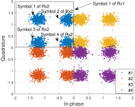
(a) Baseline-1, $\alpha=0.5$

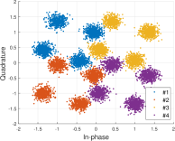
(b) Baseline-2, $\alpha=0.5$

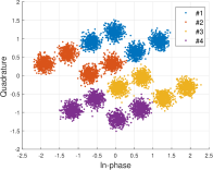
(c) DAE-ZIC, $\alpha=0.5$

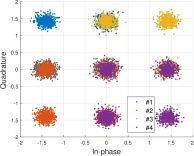
(d) Baseline-1, $\alpha=1$

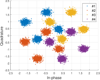
(e) Baseline-2, $\alpha=1$

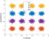
(f) DAE-ZIC, $\alpha=1$

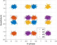
(g) Baseline-1, $\alpha=2$

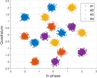
(h) Baseline-2, $\alpha=2$

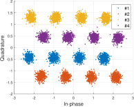
(i) DAE-ZIC, $\alpha=2$

Figure 8: Constellation of th DAE-ZIC and baselines at Rx1 for three values of $\alpha$. The colors distinguish different symbols. Each of the four clusters of the same color are caused by one of the four symbols from the interference with different noise.

VI-A Network Ablation Study

In this section, we conduct an ablation study to analyze the impact of network design and training parameters. Specifically, we investigate the effects of incorporating residual connections and selecting various training parameters. To this end, we design and perform six ablation experiments, which are detailed in Table I. The first experiment (Exp. 1) examines the presence or absence of shortcuts in the proposed method. Through Exp. 2 to Exp. 5, we investigate the impact of feeding or not feeding the training parameter $\sqrt{\alpha}$ into different sub-networks at the transmitters and receives. Exp. 6 explores the importance of Sub-network 2 which is a new design to perform power allocation.

TABLE I: Ablation settings and their performance for different values of $\alpha$.

Settings	Proposed	Exp. 1	Exp. 2	Exp. 3	Exp. 4	Exp. 5	Exp. 6
Use shortcuts	✓	-	✓	✓	✓	✓	✓
$\sqrt{\alpha}$ to sub-net 1	✓	✓	-	✓	-	✓	✓
$\sqrt{\alpha}$ to sub-net 2	✓	✓	✓	-	-	✓	-
$\sqrt{\alpha}$ to the Rx	✓	✓	✓	✓	✓	-	✓
Use sub-net 2	✓	✓	✓	✓	✓	✓	-
Performance	Proposed	Exp. 1	Exp. 2	Exp. 3	Exp. 4	Exp. 5	Exp. 6
$\alpha=0.5$	0.0252	0.0424	0.0324	0.0318	0.0340	0.0513	0.0934
$\alpha=1$	0.0236	0.1207	0.0294	0.0288	0.0281	0.0488	0.0391
$\alpha=1.5$	0.0212	0.1288	0.0253	0.0237	0.0308	0.0463	0.0328

VI-A1 The impact of residual connections

The incorporation of residual connections into the proposed DAE has a significant impact on its performance, especially for bit inputs. The addition of these shortcuts enables the network to increase its learning capacity and improve its performance without the need for additional parameters or a wider network. Moreover, these skip connections help preserve gradients, allowing the network to learn representations at varying depths. As can be seen in the first two columns of Table I, excluding residual connections significantly increases the BER, indicating that residual connections play a crucial role in the overall performance of the proposed DAE-ZIC.

VI-A2 The impact of $\sqrt{\alpha}$ at the Txs

We develop three experiments (Exp. 2, Exp. 3, and Exp. 4) in which $\sqrt{\alpha}$ is fed into either sub-networks or non and compare their BER with the proposed network in which $\sqrt{\alpha}$ is fed into bot sub-networks. While there is not big performance difference between Exp. 2, Exp. 3, and Exp. 4, for all $\alpha$ settings, there is a significant improvement when $\sqrt{\alpha}$ is fed into both sub-networks (proposed method). Sub-network 1 primarily focuses on constellation design, whereas Sub-network 2 regulates the power of I/Q dimension. Since $\sqrt{\alpha}$ influences both the constellation layout and the power distribution, providing $\sqrt{\alpha}$ to each sub-network is essential for optimizing the overall performance of the system.

VI-A3 The impact of $\sqrt{\alpha}$ at the Rx

Exp. 5 examines the performance when $\sqrt{\alpha}$ is not fed to the decoder. This experiment emphasizes the importance of incorporating interference information at the decoder side, as otherwise the BER roughly doubles (compared to the first column).

VI-A4 The impact of Sub-network 2

Exp. 6 demonstrates the importance of Sub-network 2, which is a new design to ensure different powers at I/Q dimensions. Our simulations reveal that the DAE-designed constellations downgraded to PSK in the absence of Sub-network 2. This explains why neglecting Sub-network 2 yields results similar to the Baseline-2 which uses rotated QPSK. On the contrary, as shown by the simulations, the inclusion of Sub-network 2 allows the proposed structure to design other shapes such as pulse-amplitude keying (PAM) at each transmitter. The combination of these PAMs ultimately yields a QAM-like constellation at the receiver affected by interference. These findings further emphasize the importance of incorporating Sub-network2, as it enables effective power control across the I/Q dimensions, crucial for ensuring the proper functioning of the constellations.

VI-B Scenario I: Perfect CSI

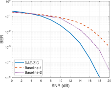
(a) ${M}_{1}={M}_{2}=4$, $\alpha=0.5$

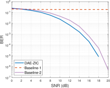
(b) ${M}_{1}={M}_{2}=4$, $\alpha=1$

(c) ${M}_{1}={M}_{2}=4$, $\alpha=1.5$

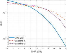
(d) ${M}_{1}={M}_{2}=8$, $\alpha=0.5$

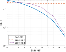
(e) ${M}_{1}={M}_{2}=8$, $\alpha=1$

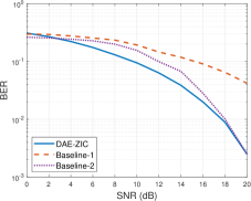
(f) ${M}_{1}={M}_{2}=8$, $\alpha=1.5$

Figure 9: The maximum (worst case) BER performance among the two users of DAE-ZIC versus SNR. The BER is averaged over different interference gains which is uniformly distributed in the given interval.

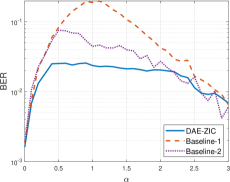
(a) ${M}_{1}={M}_{2}=4$

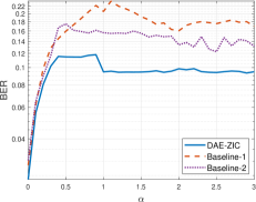
(b) ${M}_{1}={M}_{2}=8$

Figure 10: The maximum (worst case) BER performance versus interference gains. The SNR is fixed as 10dB.

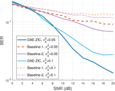
(a) ${M}_{1}={M}_{2}=4$, $\alpha=0.5$

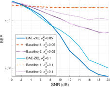
(b) ${M}_{1}={M}_{2}=4$, $\alpha=1$

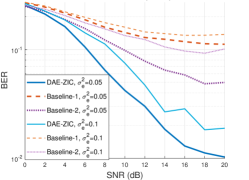
(c) ${M}_{1}={M}_{2}=4$, $\alpha=1.5$

Figure 11: The maximum (worst) BER performance among the two users versus SNR when estimation error is considered.

VI-B1 Constellation Analysis

The received constellations at Rx1 for all three methods (the two baselines and the proposed DAE-ZIC) are shown in Fig. 8. In this simulation, we set $N_{s}=2$ so that each user has $2^{N_{s}}=4$ information symbols. The channels are perfectly known, the transmit power is unity, and the SNR is 8dB.

Each sub-figure of Fig. 8 contains four four-symbol clusters differentiated by different colors. Each cluster refers to a symbol transmitted to Rx1. Within each cluster, there are four symbols, which are due to the symbols of Rx2. For example, the blue colors denote symbol $1$ of Rx1, each contaminated by one of the symbols of Rx2 (interference) and AWGN noise. It can be seen that the location and distribution of symbols are different in each method. The constellations of Baseline-1 (left column) are very crowded and even overlapped when $\alpha=1$ in Fig 8(d). This is because Tx2 strongly interferes with the transmission of Tx1 to Rx1 by directly applying 4-QAM. Baseline-2 (middle column) rotates the constellation of Tx2, which enlarges the space between symbols and thus makes the decoding easier. The proposed DAE-ZIC (right-column) creates the most separable constellations. It can better make use of the I/Q plane in constellation design based on the interference intensity. The two cooperating DAEs can intelligently choose and adjust various scaled constellation types to avoid constellation overlapping. When $\alpha=0.5$, the DAE-ZIC designs parallelogram-shape constellations compared with the square-shape constellations in the baselines. For $\alpha=1$, both the constellation of both Tx1 and Tx2 morph to PAM. The two PAM constellations are perpendicular to each other hence the overlapping is eliminated. When $\alpha=2$, Tx1 uses a parallelogram-shape QAM and Tx2 uses a PAM. By adapting their constellations to the interference intensity, the two DAEs cooperate to avoid constellation overlap as much as possible. This is the main reason that the DAE-ZIC outperforms the baselines.

In addition, compared with [26], where the symbols exhibit nearly equal power in one stream, our design allows the I/Q domains to have different power levels by incorporates sub-network 2. With this, the transmitter can generate QAM-like constellations, further mitigating the impact of interference. It is also worth noting that imperfect CSI is not considered in [26], we will show in the next section.

VI-B2 BER Performance of the DAE-ZIC

To evaluate the effectiveness of the DAE-ZIC, we compare the BER of the three methods over SNR in $[0,20]$dB and $0\leq\alpha\leq 3$. For the DAE-ZIC, we divide interval $\alpha\in[0,3]$ in to six sub-intervals, i.e, $[0,0.5)$, $[0.5,1)$, $\ldots$, $[2.5,3]$. For each sub-interval of $\alpha$, we train a DAE-ZIC through Algorithm 1.

The BER versus the SNR is shown in Fig. 9. In each sub-figure, $\alpha$ is a fixed value. In general, the DAE-ZIC outperforms the two baseline models, especially in moderate and strong interference regimes. With $N_{s}=3$, performance of DAE-ZIC drops at 0dB. The reason is we have trained the network at $\textmd{SNR}=10$dB but have tested it for a range of SNRs from 0 to 20dB. A potential way to improve is to train the DAE-ZIC with a variety of SNRs.

The BER performance versus $\alpha$ at $\textmd{SNR}=10$dB is shown in Fig. 10. In Fig. 10(a) and Fig. 10(b), we set $N_{s}=2$ and $N_{s}=3$, i.e., ${M}_{1}={M}_{2}=4$ and ${M}_{1}={M}_{2}=8$. When interference is very weak, i.e., $\alpha\in[0,0.25]$, the three methods have similar BERs. The proposed DAE-ZIC noticeably reduces the BER in weak, moderate, and strong interference cases, where $\alpha\in[0.5,2]$. From Fig. 10(a), using DAE-ZIC over $\alpha\in[0,3]$, BER is reduced 75.7% and 44.29% with respect to Baseline-1 and Baseline-2, respectively. When $\alpha\in[0.5,2]$, the improvement becomes 80.3% and 51.5%. When the interference is very strong, e.g., $\alpha>2.5$, Baseline-2 slightly outperforms the DAE-ZIC. The reason could be that 4-QAM with rotation may achieve optimal performance [16]. For $N_{s}=3$ in Fig. 10(b), 44.4% and 31.5% BER reduction is reached by the DAE-ZIC over $\alpha\in[0,3]$. For $\alpha\in[0.5,2]$, DAE-ZIC outperforms the other two methods with 45.0% and 33.4%. Baseline-1 performs poorly for $\alpha\in[0.5,2]$, because the two added QAM constellations may get crossed and overlap. Thus, Rx1 cannot decode its message. Such a phenomenon is alleviated in Baseline-2 which simply rotates one QAM constellation and the added constellations still have a reasonable symbol distance. The normalization layer allows the DAE-ZIC to design constellations without any regular-shape restrictions. Thus, the minimum distance at receivers can be enlarged which results in a lower BER.

VI-C Scenario II: Imperfect CSI

The influences of the imperfect CSI on the BER performance are shown as follows. Two types of imperfection are analyzed independently: CSI estimation error and quantization error. For imperfect CSI, both baselines use the system model in Fig. 5(b). When decoding, Rx1 will take $\theta_{\delta}$ into decoding. The performance of the two baselines and the proposed DAE-ZIC are evaluated for $\alpha\in[0,3]$ and SNR in $[0,20]$dB. In the simulation, the actual direct channel $h_{ii}\sim\mathcal{CN}(1,0.1)$ where $i\in\{1,2\}$. The estimation error $\varepsilon_{ij}$s are in $\mathcal{CN}(0,\sigma_{E}^{2})$. Then the estimated channels are obtained from (19). To be fair to the users, we use the maximum (worst) BER between them as the measurement. Each result is averaged over 500 random channels.

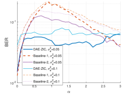
(a) ${M}_{1}={M}_{2}=4$

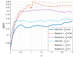
(b) ${M}_{1}={M}_{2}=8$

Figure 12: The maximum (worst) BER performance of the two users under the estimation error. The SNR is fixed as 10dB.

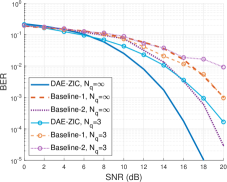
(a) ${M}_{1}={M}_{2}=4$, $\alpha=0.5$

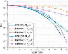
(b) ${M}_{1}={M}_{2}=4$, $\alpha=1$

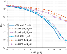
(c) ${M}_{1}={M}_{2}=4$, $\alpha=1.5$

Figure 13: The maximum (worst) BER performance of the two users versus SNR. The quantization is considered while free from estimation error.

VI-C1 CSI with Estimation Error

The BER versus interference intensity $\alpha$ is shown in Fig. 12. Two levels of the estimation error are examined. Specifically, $\sigma_{E}^{2}\in\{0.05,0.1\}$. The proposed DAE-ZIC outperforms the baselines almost for any $\alpha$. The percentage of the BER reduction is shown in Table II. With a fixed $\alpha$, the BER versus SNR is shown in Fig. 11 for weak, moderate, and strong interference. Compared to the baseline methods, the DAE-ZIC has a remarkable improvement in BER performance in all interference and estimation error levels. As mentioned earlier, the main difference between the proposed DAE-ZIC and the baselines is that the network is able to re-design the constellation based on the interference intensity, and that is how the DAE-ZIC reduces the BER.

TABLE II: BER Reductions of DAE-ZIC Compared to the Baseline Methods (in Percentage and $\alpha\in[0,3]$).

Compared to		Baseline-1		Baseline-2
$N_{s}$		2	3	2	3
$\sigma_{E}^{2}$	$0$	75.77%	44.29%	44.43%	31.50%
	$0.05$	55.40%	38.97%	39.12%	31.43%
	$0.1$	48.83%	35.81%	41.41%	29.24%

VI-C2 CSI with Feedback Quantization

When channel estimation is perfect, the BER performance with feedback quantization (with ${N_{q}=3}$) and without quantization (${N_{q}=\infty}$) is shown in Fig. 13. The DAE-ZIC outperforms the baselines with and without feedback quantization. In addition, the quantization error increases the BER of all methods. However, the performance degradation of the DAE-ZIC is much less than the other two methods. Especially, for $\alpha=1$ and $\alpha=1.5$), where the interference is strong, the DAE-ZIC outperform other methods by more than two orders of magnitude when $N_{q}=3$ and $\rm SNR=20$dB. Interestingly, Baseline-1 performs better for $N_{q}=3$ compared to $N_{q}=\infty$. The reason is that quantization of the angles may introduce rotation angle on Tx2, acting like Baseline-2 unintentionally. This then reduces the constellation overlapping and thus a better BER is reached.

With high interference intensities, i.e, $\alpha=1$ and $\alpha=1.5$, the BER of the DAE-ZIC with quantization ($N_{q}=3$) is only slightly degraded compared to the un-quantized case ($N_{q}=\infty$). This is because, while Txs receive the quantized CSI, Rx1 knows CSI before and after quantization. Then, it can to some extent correct the imperfectness in transmitters. Therefore, there is no dramatic degradation for the DAE-ZICs. On the other hand, Baseline-2 is more sensitive to the quantization error and thus a big gap of the BER happens between $N_{q}=\infty$ and $N_{q}=3$. The reason is that Baseline-2 only rotates the constellation in Tx2, which highly depends on the phase shifted by the channels.

VII Conclusion

A novel DAE architecture for interference mitigation in the two-user ZIC with perfect and imperfect CSI has been proposed. The DAE-ZIC minimizes the BER by jointly designing transmit and receive DAEs and optimizing them together. In this architecture, the average power constraint is realized by designing a normalization layer. This enables the proposed DAE-ZIC to design more efficient symbols to achieve lower BERs. BER simulations verify the effectiveness of the proposed structure. We have compared the proposed DAE-ZIC with two baseline models, and the DAE-ZIC outperforms both. With quantized CSI, the gain obtained by the DAE-ZIC compared to the best conventional method is remarkable and can be as large as two orders of magnitude at $\rm SNR=20dB$. Getting back to the questions asked in the introduction, we conclude that autoencoder is a viable solution for interference channels and it outperforms the conventional methods by designing new, nonuniform constellations which make the symbols separable at the interfered receiver side.

Xinliang Zhang (S’19) received the B.Eng. and M.Eng. degrees in Electrical Engineering from Xidian University, Xi’an, China, in 2015 and 2018, respectively. He obtained the Ph.D. degree from the Department of Electrical and Computer Engineering, Villanova University in 2022. His research interests lie in physical layer security, machine learning for wireless communications, MIMO networks, and signal processing.

Mojtaba Vaezi (S’09–M’14–SM’18) received the B.Sc. and M.Sc. degrees from Amirkabir University of Technology (Tehran Polytechnic) and the Ph.D. degree from McGill University, all in Electrical Engineering. From 2015 to 2018, he was with Princeton University as a Postdoctoral Research Fellow and Associate Research Scholar. He is currently an Associate Professor of ECE at Villanova University. Before joining Princeton, he was a researcher at Ericsson Research in Montreal, Canada. His research interests include the broad areas of signal processing and machine learning for wireless communications with an emphasis on physical layer security and sixth-generation (6G) radio access technologies. Among his publications in these areas is the book Multiple Access Techniques for 5G Wireless Networks and Beyond (Springer, 2019). Dr. Vaezi has held editorial positions at various IEEE journals, currently serving as an Editor for IEEE Transactions on Communications along with his role as a Senior Editor for IEEE Communications Letters and Senior Area Editor for IEEE Signal Processing Letters. He is a recipient of several academic, leadership, and research awards, including McGill Engineering Doctoral Award, IEEE Larry K. Wilson Regional Student Activities Award in 2013, the Natural Sciences and Engineering Research Council of Canada (NSERC) Postdoctoral Fellowship in 2014, Ministry of Science and ICT of Korea’s best paper award in 2017, IEEE Communications Letters Exemplary Editor Award in 2018, the 2020 IEEE Communications Society Fred W. Ellersick Prize, the 2021 IEEE Philadelphia Section Delaware Valley Engineer of the Year Award, and the National Science Foundation (NSF) CAREER Award in 2023.

References

- [1] X. Zhang and M. Vaezi, “Deep autoencoder-based Z-interference channels,” in Proc. Wireless Communications and Networking Conference (WCNC), pp. 1–6, 2023.
- [2] X. Zhang, M. Vaezi, and L. Zheng, “Interference-aware constellation design for Z-interference channels with imperfect CSI,” in Proc. IEEE International Conference on Communications (ICC), pp. 1–6, 2023.
- [3] A. Carleial, “A case where interference does not reduce capacity (corresp.),” IEEE Transactions on Information Theory, vol. 21, no. 5, pp. 569–570, 1975.
- [4] H. Sato, “The capacity of the Gaussian interference channel under strong interference,” IEEE Transactions on Information Theory, vol. 27, no. 6, pp. 786–788, 1981.
- [5] T. Han and K. Kobayashi, “A new achievable rate region for the interference channel,” IEEE Transactions on Information Theory, vol. 27, no. 1, pp. 49–60, 1981.
- [6] I. Sason, “On achievable rate regions for the Gaussian interference channel,” IEEE transactions on information theory, vol. 50, no. 6, pp. 1345–1356, 2004.
- [7] R. H. Etkin, D. N. Tse, and H. Wang, “Gaussian interference channel capacity to within one bit,” IEEE Transactions on Information Theory, vol. 54, no. 12, pp. 5534–5562, 2008.
- [8] A. S. Motahari and A. K. Khandani, “Capacity bounds for the Gaussian interference channel,” IEEE Transactions on Information Theory, vol. 55, no. 2, pp. 620–643, 2009.
- [9] X. Shang, G. Kramer, and B. Chen, “A new outer bound and the noisy-interference sum–rate capacity for Gaussian interference channels,” IEEE Transactions on Information Theory, vol. 55, no. 2, pp. 689–699, 2009.
- [10] V. S. Annapureddy and V. V. Veeravalli, “Gaussian interference networks: Sum capacity in the low-interference regime and new outer bounds on the capacity region,” IEEE Transactions on Information Theory, vol. 55, no. 7, pp. 3032–3050, 2009.
- [11] Y. Wu, C. Xiao, X. Gao, J. D. Matyjas, and Z. Ding, “Linear precoder design for MIMO interference channels with finite-alphabet signaling,” IEEE Transactions on Communications, vol. 61, no. 9, pp. 3766–3780, 2013.
- [12] G. Foschini, R. Gitlin, and S. Weinstein, “Optimization of two-dimensional signal constellations in the presence of Gaussian noise,” IEEE Transactions on Communications, vol. 22, no. 1, pp. 28–38, 1974.
- [13] G. Forney, R. Gallager, G. Lang, F. Longstaff, and S. Qureshi, “Efficient modulation for band-limited channels,” IEEE Journal on Selected Areas in Communications, vol. 2, no. 5, pp. 632–647, 1984.
- [14] A. J. Goldsmith and S.-G. Chua, “Variable-rate variable-power MQAM for fading channels,” IEEE Transactions on Communications, vol. 45, no. 10, pp. 1218–1230, 1997.
- [15] M. F. Barsoum, C. Jones, and M. Fitz, “Constellation design via capacity maximization,” in In Proc. IEEE International Symposium on Information Theory, pp. 1821–1825, 2007.
- [16] F. Knabe and A. Sezgin, “Achievable rates in two-user interference channels with finite inputs and (very) strong interference,” in Proc. IEEE Asilomar Conference on Signals, Systems and Computers (ACSSC), pp. 2050–2054, 2010.
- [17] A. Ganesan and B. S. Rajan, “Two-user Gaussian interference channel with finite constellation input and FDMA,” IEEE Transactions on Wireless Communications, vol. 11, no. 7, pp. 2496–2507, 2012.
- [18] Z. K. Ho and E. Jorswieck, “Improper Gaussian signaling on the two-user SISO interference channel,” IEEE Transactions on Wireless Communication, vol. 11, no. 9, pp. 3194–3203, 2012.
- [19] T. O’Shea and J. Hoydis, “An introduction to deep learning for the physical layer,” IEEE Transactions on Cognitive Communications and Networking, vol. 3, no. 4, pp. 563–575, 2017.
- [20] T. J. O’Shea, T. Erpek, and T. C. Clancy, “Deep learning based MIMO communications,” arXiv:1707.07980, 2017.
- [21] N. Nartasilpa, A. Salim, D. Tuninetti, and N. Devroye, “Communications system performance and design in the presence of radar interference,” IEEE Transactions on Communications, vol. 66, no. 9, pp. 4170–4185, 2018.
- [22] H. Ye, L. Liang, G. Y. Li, and B.-H. Juang, “Deep learning-based end-to-end wireless communication systems with conditional GANs as unknown channels,” IEEE Transactions on Wireless Communications, vol. 19, no. 5, pp. 3133–3143, 2020.
- [23] J. Song, C. Häger, J. Schröder, T. O’Shea, and H. Wymeersch, “Benchmarking end-to-end learning of MIMO physical-layer communication,” in Proc. IEEE Global Communications Conference (GLOBECOM), pp. 1–6, 2020.
- [24] X. Zhang, M. Vaezi, and T. J. O’Shea, “SVD-embedded deep autoencoder for MIMO communications,” in Proc. IEEE International Conference on Communications (ICC), pp. 1–6, 2022.
- [25] T. Erpek, T. J. O’Shea, and T. C. Clancy, “Learning a physical layer scheme for the MIMO interference channel,” in Proc. IEEE International Conference on Communications (ICC), pp. 1–5, 2018.
- [26] D. Wu, M. Nekovee, and Y. Wang, “Deep learning-based autoencoder for M-user wireless interference channel physical layer design,” IEEE Access, vol. 8, pp. 174679–174691, 2020.
- [27] S. Shamai and M. Wigger, “Rate-limited transmitter-cooperation in wyner’s asymmetric interference network,” in Proc. IEEE International Symposium on Information Theory Proceedings, pp. 425–429, 2011.
- [28] G. Kramer, “Review of rate regions for interference channels,” in Proc. IEEE International Zurich Seminar on Communications (IZSC), pp. 162–165, 2004.
- [29] M. Vaezi and H. V. Poor, “Simplified Han-Kobayashi region for one-sided and mixed Gaussian interference channels,” in Proc. IEEE International Conference on Communications (ICC), pp. 1–6, 2016.
- [30] C. Lameiro, I. Santamaría, and P. J. Schreier, “Rate region boundary of the SISO Z-interference channel with improper signaling,” IEEE Transactions on Communications, vol. 65, no. 3, pp. 1022–1034, 2016.
- [31] N. Deshpande and B. S. Rajan, “Constellation constrained capacity of two-user broadcast channels,” in Proc. IEEE Global Telecommunications Conference (GLOBECOM), pp. 1–6, 2009.
- [32] F. Chollet, J. Allaire, et al., “R interface to KERAS.” https://github.com/rstudio/keras, 2017.
- [33] Y. Chen and C. Tellambura, “Performance analysis of maximum ratio transmission with imperfect channel estimation,” IEEE Communications Letters, vol. 9, no. 4, pp. 322–324, 2005.