Low-depth Clifford circuits approximately solve MaxCut

Abstract

We introduce a quantum-inspired approximation algorithm for MaxCut based on low-depth Clifford circuits. We start by showing that the solution unitaries found by the adaptive quantum approximation optimization algorithm (ADAPT-QAOA) for the MaxCut problem on weighted fully connected graphs are (almost) Clifford circuits. Motivated by this observation, we devise an approximation algorithm for MaxCut, ADAPT-Clifford, that searches through the Clifford manifold by combining a minimal set of generating elements of the Clifford group. Our algorithm finds an approximate solution of MaxCut on an $N$-vertex graph by building a depth $O(N)$ Clifford circuit, with worst-case runtime and space complexities $O(N^{6})$ and $O(N^{2})$, respectively. We implement ADAPT-Clifford and characterize its performance on graphs with positive and signed weights. The case of signed weights is illustrated with the paradigmatic Sherrington-Kirkpatrick model, for which our algorithm finds solutions with ground-state mean energy density corresponding to $\sim 94\%$ of the Parisi value in the thermodynamic limit. The case of positive weights is investigated by comparing the cut found by ADAPT-Clifford with the cut found with the Goemans-Williamson (GW) algorithm. For both sparse and dense instances we provide copious evidence that, up to hundreds of nodes, ADAPT-Clifford finds cuts of lower energy than GW. Since good approximate solutions to MaxCut can be efficiently found within the Clifford manifold, we hope our results will motivate to rethink the approach so far used to search for quantum speedup in combinatorial optimization problems.

I Introduction

Quantum computation allows for information processing capacities beyond those attainable in classical digital computing, provided that fault-tolerant quantum computers can be built in practice [1]. While the milestone of break-even error correction of a single logical qubit has been reached [2, 3, 4], the roadmap to scalable fault-tolerant quantum processors extends into the long term. At the same time, the level of noise in near-term quantum devices with modest numbers of qubits precludes their use as general-purpose machines [5, 6].

On the other hand, near-term quantum processors have found a niche in the hybrid quantum-classical model of computation with Variational Quantum Algorithms (VQAs) [7, 8, 9]. These algorithms perform classical optimization of a problem-specific objective function that is evaluated by measuring the output of a parametrized quantum circuit. Through variational search over circuit parameters, a VQA thus seeks a solution circuit that transforms a simple input state in the Hilbert space of problem variables to a superposition of approximate solutions, i.e., configurations that yield near-optimal values of the objective function. In attempts to determine whether they can lead to a speedup over classical algorithms for any useful task, VQAs have been applied to a variety of combinatorial optimization problems. Quantum approximate optimization algorithms (QAOAs) [10, 11] have been in a constant tug of war with classical solvers, with initial indications of putative quantum speedups [12, 13, 14, 15], followed by experimental claims [16] and rebuttals [17], and then further proposals for possible quantum speedup [18]. A byproduct of this large effort has been the definition and construction of quantum-inspired algorithms [19, 20, 21, 22, 23, 24]. These are “dequantized” classical versions of quantum or hybrid quantum-classical algorithms that unveil and exploit previously unrecognized properties or structures in a problem, leading to solution strategies that outperform the best known classical algorithm.

In this work, we introduce a quantum-inspired approximation algorithm for the MaxCut problem. The algorithm, which we dub ADAPT-Clifford, is motivated by the observation that the solution circuits found by an adaptive QAOA variant for MaxCut on weighted complete graphs are (almost) Clifford circuits, a well-known restricted class of quantum circuits that are easy to simulate classically [25, 26, 27, 28, 29]. ADAPT-Clifford builds an entangled state with a number of unitary operations that is equal to the number of nodes $N$, adding at every step a known two-qubit gate to the circuit. The algorithm is polynomial both in time and space, with worst case runtime complexity $O(N^{6})$ and space complexity $O(N^{2})$. We characterize the performance of the algorithm in several families of graphs. For graph sizes up to $N=30$ nodes we report the exact approximation ratios. For larger problem sizes up to hundreds of nodes and depending on graph family, we assess the performance by either direct comparison with the solution found by the best classical algorithm for MaxCut [30, 31], or by comparing with the known value of the mean energy density in the thermodynamic limit.

The rest of this manuscript is organized as follows. In Sec. II we present a short summary of the MaxCut problem, quantum approximate optimization and its adaptive variant, Clifford circuits, and introduce the tools we use to characterize the structure of solution circuits. In Sec. III we present the origin of the algorithm by analyzing the structure of solution circuits to MaxCut on weighted complete graphs obtained with QAOA and ADAPT-QAOA. In Sec. IV we present the ADAPT-Clifford algorithm, discuss its details, and analyze its runtime and space complexities in different types of graphs. In Sec. V we present numerical results of the algorithm performance on weighted complete graphs with positive and signed weights, using the Sherrington-Kirkpatrick model as a specific example of the latter. In Sec. VI we explore the performance of the algorithm beyond complete graphs, including weighted and unweighted $K$-regular graphs and Erdös-Rényi graphs. Finally in Sec. VII we conclude with a discussion of our results in the context of near-term quantum optimization algorithms and present an outlook of future work.

II Background and methods

II.1 The MaxCut problem

Given a graph $\mathcal{G}=(\mathcal{V},\mathcal{E})$, where $\mathcal{V}$ is the vertex set and $\mathcal{E}\subseteq\mathcal{V}^{2}$ is the set of edges ($\mathcal{E}=\mathcal{V}^{2}$ is a complete graph), and edge weights $\omega_{i,j}\in\mathbb{R}$ for $(i,j)\in\mathcal{E}$, the MaxCut problem asks to partition $\mathcal{V}$ into two complementary subsets $\mathcal{A},\overline{\mathcal{A}}\subset\mathcal{V}$, such that the total weight of the edges between $\mathcal{A}$ and $\overline{\mathcal{A}}$ is maximized. We use binary variables $z_{i}\in\{0,1\}$, $i\in\mathcal{V}$ to help us identify each subset, so that $z_{i}=1$ if vertex $i\in\mathcal{A}$ and $z_{i}=0$ if $i\in\overline{\mathcal{A}}$. The maximal cut can then be formally expressed as the assignment $\mathbf{z}^{\prime}$ that maximizes the cost function

$$C(\mathbf{z})=\sum_{(i,j)\in\mathcal{E}}\omega_{i,j}z_{i}(1-z_{j}),$$ (1)

where $\mathbf{z}=z_{1}...z_{N}$ is a $N$-bit binary string and $\omega_{i,j}=\omega_{j,i}$ $\forall(i,j)\in\mathcal{E}$.

The MaxCut problem on general graphs is known to be NP-hard [32]. However, MaxCut can be solved in polynomial time in some special cases, such as graphs without long odd cycles [34], weakly bipartite graphs [35], planar graphs both weighted [36, 37] and unweighted [38, 39], $1$-planar graphs [40], and graphs with $k$ crossings [41]. Finally, when all the edge weights are negative, MaxCut becomes a equivalent to MinCut and admits a polynomial time algorithm [42].

Beyond the special cases mentioned above and due to the difficulty of solving the problem exactly, one often aims instead to find approximation algorithms that yield reasonably good solutions in polynomial time for all problem instances. That is, we search for an algorithm that outputs an assignment $\mathbf{z}^{*}$, such that the approximation ratio

$$\alpha(\mathbf{z}^{*})=\frac{C(\mathbf{z^{*}})}{\underset{\mathbf{z}}{{\rm max}}[C(\mathbf{z})]},$$ (2)

equals some desired value, ideally as close to $1$ as possible, on all instances of MaxCut. However, in some cases the gap between approximate an optimal solutions cannot be reduced arbitrarily in polynomial time [43], a phenomenon known as hardness of approximation. For MaxCut on general graphs, the best known approximation algorithm is that of Goemans and Williamson (GW) [30], which has a performance guarantee (worst case) of $\alpha\simeq 0.878$ [30, 44, 31] . Below we will present extensive performance comparisons between ADAPT-Clifford and the GW algorithm, in order to be as self contained as possible we review the details of the GW algorithm in App. A.

One might hope to achieve better approximation ratios by focusing on specific families of graphs. For unweighted graphs Ref. [46] showed that finding an algorithm yielding an approximation ratio better than $16/17$ is NP-hard. Nearly optimal algorithms both for cubic graphs [47], guaranteeing $\alpha=0.9326$, and for $K$-regular graphs of large degree [48], are known. Another interesting example is the case of dense graphs, i.e., graphs with $O(N^{2})$ edges. Polynomial time approximation schemes (PTAS) are known for both unweighted [49, 50] and weighted [51] graphs, although for the latter there is only an existence result. A PTAS guarantees an approximate solution whose cost is $1-\epsilon$ away from the optimal. Although these schemes have a provable polynomial runtime in $N$, it might not be polynomial in $\epsilon$, see for example Ref. [50]. We will come back to this point in Sec. VII.

In quantum approximate optimization, the objective function of a combinatorial optimization problem defined on binary variables $z_{i}$, such as MaxCut, is expressed as an Ising Hamiltonian through the mapping $\sigma_{i}=2z_{i}-1$, with connectivity dictated by the graph $\mathcal{G}$ [52]. That is, the entries $\omega_{i,j}$ of the adjacency matrix reflect the coupling between the $i$-th and $j$-th spin. In this setting the optimum $\mathbf{z}^{\prime}$ is encoded as the ground state of the Ising Hamiltonian. The Ising Hamiltonian is then promoted to a Hamiltonian operator via the identification $\sigma_{i}\to Z_{i}$, with $Z_{i}$ a Pauli-$z$ operator acting on the qubit that corresponds to the $i$-th spin. For the MaxCut problem, the corresponding Hamiltonian is

$$H_{\rm C}=\frac{1}{2}\sum_{i<j}\omega_{i,j}Z_{i}Z_{j}.$$ (3)

In writing Eq. (3) we have dropped a constant factor equal to $\sum_{i<j}\frac{\omega_{i,j}}{2}$ and added a minus sign to turn the maximization problem defined by Eq. (1) into a minimization one.

In analogy with classical approximation algorithms, quantum approximate optimization yields approximate solutions in the form of a state $|\phi\rangle$, whose energy expectation is as close as possible to the ground-state energy of the Ising Hamiltonian. Thus, the approximation ratio, Eq. (2), takes the form

$$\alpha=\frac{\langle\phi|H_{\rm C}|\phi\rangle}{E^{\rm C}_{\rm min}},$$ (4)

where $E^{\rm C}_{\rm min}$ is the smallest eigenvalue of $H_{\rm C}$. To achieve advantageous performance, a quantum algorithm must produce an approximate solution with a desired $\alpha$ faster than any classical algorithm.

II.2 The quantum approximate optimization algorithm and its adaptive variant

The Quauntum Approximated Optimization Algorithm (QAOA) is a type of variational algorithm [8] that aims to solve combinatorial optimization problems [10]. It is defined by a parametrized quantum circuit with a periodic structure. Each layer of the circuit is given by a product of two unitaries, time evolution under $H_{\rm C}$, followed by time evolution under a mixer Hamiltonian

$$H_{\rm M}=\sum_{j=1}^{N}X_{j},$$ (5)

where $X_{j}$ is a Pauli-$x$ on the $j$-th qubit. For $p$ layers QAOA prepares the state

$$|\psi(\boldsymbol{\gamma},\boldsymbol{\beta})\rangle_{p}=\left[\prod_{l=1}^{p}e^{-i\beta_{l}H_{\rm M}}e^{-i\gamma_{l}H_{\rm C}}\right]\mathrm{H}^{\otimes N}|0\rangle^{\otimes N},$$ (6)

where $\boldsymbol{\gamma}=\gamma_{1},...,\gamma_{p}$, $\boldsymbol{\beta}=\beta_{1},...,\beta_{p}$, and $\mathrm{H}$ is the Hadamard gate. In order to find approximate solutions the set of $2p$ parameters is optimized so as to minimize $\langle\psi(\boldsymbol{\gamma},\boldsymbol{\beta})|H_{\rm C}|\psi(\boldsymbol{\gamma},\boldsymbol{\beta})\rangle_{p}$. After executing the circuit with optimized parameters a measurement in the computational basis returns a candidate solution in the form of a bit string $\mathbf{z}^{*}$. Ideally, one would sample with high probability a good approximate solution. We will denote the optimal parameters found by numerical experiments as $(\boldsymbol{\gamma}^{*},\boldsymbol{\beta}^{*})$, and the associated solution unitary $U(\boldsymbol{\gamma}^{*},\boldsymbol{\beta}^{*})=\prod_{l=1}^{p}e^{-i\beta^{*}_{l}H_{\rm M}}e^{-i\gamma^{*}_{l}H_{\rm C}}$.

Not much is known regarding performance guarantees and hardness of approximation for QAOA. The case of constant $p$ has so far been the main focus, as it is the regime of interest for current quantum devices [5]. Ref. [53] gives evidence for a possible quantum advantage for MaxCut on $3$-regular graphs with shallow QAOA. At the same time, it is known that constant $p$ QAOA is bounded away from optimality in sparse graphs [54, 55, 56], as well as in some dense problems where the overlap gap property  is known to exist [58]. These results were recently extended to the case of $p\sim\log(N)$ [59]. However these results do not apply directly to the case of $p\sim{\rm poly}(N)$. As a consequence there are no conclusive results on the runtime required for $p\sim{\rm poly}(N)$ QAOA to reach a given approximation ratio, with only loose lower bounds appearing recently [60]. Most studies of QAOA so far have been numerical experiments, meaning that indications of a putative advantage [12], have been inconclusive due to the small problem sizes accessible to either quantum implementations or classical simulation.

To alleviate some of the roadblocks explored above, variants to the original QAOA ansatz have been developed, see Ref. [62] for a review. Of interest to us here is the ADAPT [63] variant, which was proposed as a way to find ansätze which are tailored to the specifics of the problem under consideration. ADAPT-QAOA is an iterative variational algorithm which replaces the fixed mixer Hamiltonian in Eq. (6), by a suitably chosen one, $A_{l}$, at each layer $l\leq p$. Thus, $p$-layer ADAPT-QAOA prepares the state

$$|\psi(\gamma,\beta)\rangle_{p}^{\rm ADAPT}=\left[\prod_{l=1}^{p}e^{-i\beta_{l}A_{l}}e^{-i\gamma_{l}H_{\rm C}}\right]\mathrm{H}^{\otimes N}|0\rangle^{\otimes N}.$$ (7)

The $l$-th mixer Hamiltonian is chosen as the one which maximizes the energy gradient, that is,

$$A_{l}=\underset{A_{s}\in\mathrm{P}_{\rm OP}}{\rm max}\left[-i\langle\psi_{l-1}|e^{i\gamma_{l}H_{\rm C}}[H_{\rm C},\hat{A}_{s}]e^{-i\gamma_{l}H_{\rm C}}|\psi_{l-1}\rangle\right],$$ (8)

where the new variational parameter $\gamma_{l}$ is set to a predefined small positive value $\gamma_{0}\sim 0$ [63], and $\mathrm{P}_{\rm OP}$ is an operator pool. The choice of pool is not unique, with different pools being advantageous in different situations [64, 65]. Below we restrict ourselves to the pool

$$\begin{split}\mathrm{P}_{\rm OP}=&\{\sum_{i}X_{i},\sum_{i}Y_{i}\}\cup\{X_{j},Y_{j}\}_{j=1,...,N}\\ &\cup\{X_{j}X_{k},Y_{j}Y_{k},Y_{j}Z_{k},Z_{j}Y_{k}\}_{j,k=1,...,N,j\neq k},\end{split}$$ (9)

which is sufficient for our purposes.

In contrast to QAOA, ADAPT-QAOA grows the circuit layer by layer, until the desired number $p$. As such, we begin with a single layer, find the corresponding mixer according to Eq. (8), then optimize to find the best parameters. We then add a second layer, find the corresponding mixer according to Eq. (8), initialize the new pair of parameters to zero , the rest of the parameters to the best values already found, and optimize all of them. This procedure is repeated until $p$ layers are added. For a fair comparison between QAOA and ADAPT-QAOA in our numerical simulations we construct the QAOA solution circuit following the same iterative strategy, but with a fixed mixer.

II.3 Clifford circuits and their efficient simulation

In this subsection we review some concepts of the stabilizer formalism which will be used later in the manuscript. For a general presentation see Ref. [1].

The single qubit Pauli group is given by the operators $\{\mathbb{I},X,Y,Z\}$ together with multiplicative factors $\pm 1,\pm i$. The $N$ qubit Pauli group $\mathcal{\tilde{P}}_{N}$ is given by all the $N$-tensor products of these operators together with multiplicative factors. Given a pure state on $N$ qubits $|\psi\rangle$, we say $\tilde{P}_{i}\in\mathcal{\tilde{P}}_{N}$ stabilizes $|\psi\rangle$ if the state is an eigenvector of $\tilde{P}_{i}$ with eigenvalue $+1$: $\tilde{P}_{i}|\psi\rangle=|\psi\rangle$. A $n$-qubit pure state is a stabilizer state if it can be completely specified, up to a global phase, by its $N$ stabilizers.

Quantum circuits which map stabilizer states to stabilizer states define a large class of nontrivial quantum circuits —stabilizer circuits— which can be simulated in polynomial time on a classical computer [28, 29]. This is the content of the celebrated Gottesman-Knill theorem [26, 27]. These quantum circuits can be completely written in terms of controlled-NOT, Hadamard, and phase gates, and single qubit measurements. Importantly, the efficient classical simulability does not imply these circuits are not interesting. On the contrary, they have extensive applications in quantum information science, for instance encoding and decoding in quantum error correction [67, 68, 25, 27], dense quantum coding [69], quantum teleportation [70], quantum simulation [71, 72], proof of principle of quantum advantage with nonlocal games [73, 74], as well as in quantum many-body physics [75, 76, 77, 78, 79].

In absence of measurements, stabilizer circuits are referred to as Clifford circuits or Clifford unitaries. They form a group $\mathcal{C}$, defined as the unitaries which normalize the Pauli group, that is, the unitaries which map Pauli operators to Pauli operators. Following from the Gottesman-Knill theorem, this group has three generators, the controlled-NOT, Hadamard, and phase gates. Naturally the Pauli operators are elements of the group, as they are generated by Hadamard and phase.

Both the QAOA and ADAPT-QAOA ansätze are defined as products of unitaries generated by Pauli strings. When are unitary transformations generated by Pauli strings Clifford unitaries? To answer this question, take $\tilde{P}_{i},\tilde{P}_{j}\in\mathcal{\tilde{P}}$, two distinct Pauli strings that either commute or anticommute by definition. If $W(\theta)=e^{-i\theta\tilde{P}_{j}}$, then $W^{\dagger}\tilde{P}_{i}W=\tilde{P}_{i}$ if $[\tilde{P}_{i},\tilde{P}_{j}]=0$, and $W^{\dagger}\tilde{P}_{i}W=i\tilde{P}_{i}\tilde{P}_{j}$ if $\{\tilde{P}_{i},\tilde{P}_{j}\}=0$ and $\theta=\pm m\frac{\pi}{4}$ with $m\in\mathbb{N}$. We thus see that when a quantum circuit is composed of products of unitaries generated by Pauli strings that do not necessarily commute, it is a Clifford circuit if an only if the parameters of these transformations are integer multiples of $\pm\pi/4$. Therefore, if QAOA solution circuits $U(\boldsymbol{\gamma}^{*},\boldsymbol{\beta}^{*})$ are to be Clifford, then the circuit parameters $\boldsymbol{\gamma}^{*}$ and $\boldsymbol{\beta}^{*}$ must be integer multiples of $\pm\pi/4$.

II.4 Characterizing the structure of solution unitaries

Here we introduce the tools we use in the next section to characterize the structure of QAOA solution circuits $U(\boldsymbol{\gamma}^{*},\boldsymbol{\beta}^{*})$. Consider the Hilbert space $\mathcal{H}$ of $N$ qubits with dimension $d=2^{N}$, and define the $N$-qubit Pauli basis as $\mathcal{P}_{N}=\mathcal{\tilde{P}}_{N}/\langle\pm i\mathbb{I}\rangle$, the quotient group containing, $D=4^{N}-1$, Pauli strings with all multiplicative factors equal to $+1$. Furthermore any pair of Pauli strings obey ${\rm Tr}[P_{i}P_{j}]=d\delta_{ij}$. Therefore, $\mathcal{P}_{N}$ defines a basis for all Hermitian operators in $\mathcal{H}$.

Consider some Hermitian operator $O$ acting on $\mathcal{H}$. If $O$ evolves under some unitary transformation $V$, we write

$$O^{\prime}=V^{\dagger}OV=\sum_{j=1}^{D}f[P_{j};O^{\prime}]P_{j},$$ (10)

with $P_{j}\in\mathcal{P}_{N}$. Noticing that $\sum_{j}|f[P_{j};O^{\prime}]|^{2}={\rm Tr}[O^{\prime 2}]={\rm Tr}[O^{2}]$, we define

$$p_{j}(O;V)=\frac{1}{{\rm Tr}[O^{2}]}|f[P_{j};O^{\prime}]|^{2}.$$ (11)

It is easy to see that $\sum_{j}p_{j}=1$. Eq. (11) thus denotes the probability of finding $O^{\prime}$ to be the $j$-th Pauli string $P_{j}$. In the case of $O=P_{l}$, the normalization factor in Eq. (11) is $\sum_{j}|f[P_{j};O^{\prime}]|^{2}=d$.

We analyze the transformation $V$ as an “input-output” channel, with $O$ the input and $O^{\prime}$ the output, and are interested in characterizing the locality, in the Pauli basis, of the output. This can be inferred from the the localization properties of $p_{j}(O;V)$, which we investigate with the Second Renyi entropy, see Ref. [80] and Sec. 2.7 of Ref. [81], 

$$\mathcal{S}\left(O;V\right)=-\log\left(\sum_{j=0}^{4^{N}}\frac{|f[P_{j};O^{\prime}]|^{4}}{d^{2}}\right).$$ (12)

The $P_{l}\in\mathcal{P}_{N}$ can be ordered by their “weight”, i.e., the number of nonidentity elements in the Pauli string. This ordering allows us to systematically study the Clifford character of the transformation $V$ on Pauli strings. Naturally, the first step will be to check it for strings of weight one, which is done by setting $O=Y_{n}$, where $Y_{n}$ denotes a Pauli operator with a Pauli-$y$ on the $n$-th qubit position and identity everywhere else. In particular we denote $\mathcal{S}\left(Y_{n};V\right)=\mathcal{S}_{n}\left(V\right)$. Since we can place the initial Pauli-$y$ at any of the $N$ positions representing the nodes of the graph, we consider the node-averaged Renyi entropy of the operator distribution

$$\overline{\mathcal{S}}\left(V\right)=\frac{1}{N}\sum_{n=1}^{N}\mathcal{S}_{n}(V),$$ (13)

as our figure of merit. Since Clifford unitaries map Pauli strings to Pauli strings, then $\mathcal{S}\left(O;V\right)=0$ for all $O\in\mathcal{P}_{N}$. Since we are only checking the behavior of $V$ as a “channel” for Pauli strings localized on one qubit, a vanishing $\overline{\mathcal{S}}$ is necessary (but not sufficient) for $V$ to be Clifford. We thus use $\overline{S}$ as a witness of Cliffordness.

We supplement this witness with an examination of the optimal parameters $(\boldsymbol{\gamma}^{*},\boldsymbol{\beta}^{*})$. Observation of $\boldsymbol{\gamma}^{*},\boldsymbol{\beta}^{*}=\pm m\frac{\pi}{4}$ with $m\in\mathbb{N}$, then provides the sufficient condition for $V$ to be Clifford. This observation is made quantitative via the distance of the vector of parameters $\mathbf{v}$ to the discrete set of interest. We define this distance as

$$\mathcal{D}(\mathbf{v})=\sum_{v_{i}\in\mathbf{v}}\frac{\underset{l\in\mathbb{Z}}{\rm min}[|v_{i}-l\frac{\pi}{4}|]}{\pi/8},$$ (14)

where the normalization ensures that each term in the sum is bounded to the interval $[0,1]$, thus we have $0\leq\mathcal{D(\mathbf{v})}\leq|\mathbf{v}|$. Then the instance averaged distances $\mathbb{E}[\mathcal{D}(\gamma^{*})]\to 0$ and $\mathbb{E}[\mathcal{D}(\beta^{*})]\to 0$ will inform us of solution circuits which are close to Clifford.

III Origin of the ADAPT-Clifford algorithm

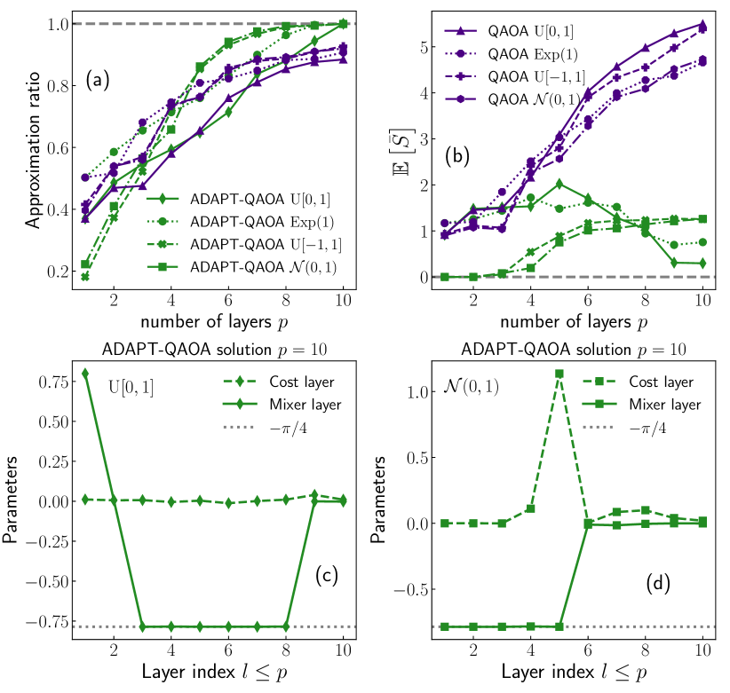
Figure 1: QAOA and ADAPT-QAOA results for MaxCut on weighted complete graphs with $N=6$. (a) Instance average of $\alpha$ for QAOA (purple) and ADAPT-QAOA (green). (b) Instance average of $\overline{\mathcal{S}}$ in Eq. 13 of solution circuits with $p$ layers fore QAOA (purple) and ADAPT-QAOA (green). For both (a) and (b) the distributions of the weights used are indicated in the figure. (c,d) Examples of the parameters $\boldsymbol{\gamma}^{*}$ (cost, solid line) and $\boldsymbol{\beta}^{*}$ (mixer, dashed line) of the solution unitary $U(\boldsymbol{\gamma}^{*},\boldsymbol{\beta}^{*})$ for an instance with weights drawn from ${\rm U}[0,1]$ (c) and $\mathcal{N}(0,1)$ (d).

To understand the origin of the ADAPT-Clifford algorithm, it is instructive to examine the solution circuits obtained with QAOA and ADAPT-QAOA for MaxCut on small weighted complete graphs. We implemented both variational algorithms in the extensible Julia framework Yao.jl [83] and use the COBYLA optimizer. The analysis of the operator distribution in the Pauil basis was implemented using QuantumOptics.jl [84].

We consider first the case of graphs with positive weights with $\omega_{i,j}$ from either ${\rm U}[0,1]$, where by ${\rm U}[a,b]$ we denote the uniform distribution in the interval $[a,b]$, or ${\rm Exp}(1)$, the exponential distribution with mean $1$. In Fig. 1a we show the mean approximation ratios for $50$ problem instances with $N=6$ for circuits up to $p=10$ layers. Similar to the observation in Ref. [63], ADAPT-QAOA (green diamonds and circles in Fig. 1a) finds a solution arbitrarily close to the exact solution at sufficiently high but finite $p$, away from the $p\to\infty$ limit where QAOA is guaranteed to reach the exact solution. In Fig. 1b we show the expectation value over instances of $\overline{\mathcal{S}}$, $\mathbb{E}[\overline{\mathcal{S}}]$. The ADAPT-QAOA solution circuits that lead to $\alpha\to 1$ in Fig. 1a display $\mathbb{E}[\overline{\mathcal{S}}]\to 0$, indicating they might be Clifford circuits. In contrast, the QAOA solution unitaries show $\mathbb{E}[\overline{\mathcal{S}}]>0$ with a tendency towards the typical value, $\log(4^{-N})$, with increasing depth, in agreement with previous works using other indicators [85, 86].

To verify the Cliffordness of the ADAPT-QAOA solution circuits we examine the optimized parameters, $(\boldsymbol{\gamma}^{*},\boldsymbol{\beta}^{*})$, at $p=10$. An example is shown in Fig. 1c where dashed and solid lines correspond to $\boldsymbol{\gamma}^{*}$ and $\boldsymbol{\beta}^{*}$, respectively. We observe $\boldsymbol{\gamma}^{*}\to 0$ and $\boldsymbol{\beta}^{*}\to-\pi/4$ in all layers, and the mixer Hamiltonians selected by the adaptive step are almost always $Y_{l}Z_{m}$ for some pair of qubits $(l,m)$. Furthermore the distances of the optimal parameters for $p=10$ to $\pm s\frac{\pi}{4}$ with $s\in\mathbb{N}$ averaged over all instances with $\alpha\to 1$ ($\omega_{i,j}\in{\rm U}[0,1]$), are $\mathbb{E}[\mathcal{D}(\gamma^{*})]=0.522\pm 0.270$ and $\mathbb{E}[\mathcal{D}(\beta^{*})]=0.247\pm 0.322$, indicating the optimized parameters are closed, on average, to the Clifford values. This is to be contrasted with $\mathbb{E}[\mathcal{D}(\gamma^{*})]=3.53\pm 0.94$ and $\mathbb{E}[\mathcal{D}(\beta^{*})]=3.41\pm 0.62$ for the optimized parameters of the QAOA solution circuits with $p=10$. Finally, we extensively checked that the properties of the ADAPT-QAOA solution unitary discussed here do not change as long as the edge weights are all positive.

Next we consider the case of signed weights with $\omega_{i,j}$ sampled either from ${\rm U}[-1,1]$ or $\mathcal{N}(0,1)$, the normal distribution with mean $0$ and variance $1$. In Fig. 1a we compare the averaged approximation ratio of the ADAPT-QAOA solutions with that of the QAOA solutions for the same problem instances. Similar to the case of strictly positive weights, ADAPT-QAOA solutions get arbitrarily close to the exact solution when enough layers are considered. As seen in Fig. 1b $\mathbb{E}[\overline{\mathcal{S}}]\neq 0$ for the ADAPT-QAOA solution (green crosses and squares). Although the circuits found are therefore not Clifford, $\mathbb{E}[\overline{\mathcal{S}}]\sim 1$ at $p=10$ for the small problem size under study, in contrast to QAOA solution circuits (purple crosses and hexagons), for which $\mathbb{E}[\overline{\mathcal{S}}]$ tends towards the typical value.

The small value of $\mathbb{E}[\overline{\mathcal{S}}]$ for the ADAPT-QAOA solutions raises the question: how far is this solution from the Clifford manifold? To answer this, in Fig. 1d we show the optimized parameters $(\boldsymbol{\gamma}^{*},\boldsymbol{\beta}^{*})$ found for one of the problem instances solved. The $\boldsymbol{\beta}^{*}$'s are either $0$ or $-\pi/4$, indicating the mixer unitaries are Clifford, with mixer Hamiltonians almost always $Y_{l}Z_{m}$ for some pair of qubits $(l,m)$, and most of the $\boldsymbol{\gamma}^{*}$'s are zero with only few, $\sim 2$, being nonzero. Furthermore, the distances of the optimized parameters for $p=10$ to $\pm s\frac{\pi}{4}$ with $s\in\mathbb{N}$ averaged over all instances with $\alpha\to 1$ ($\omega_{i,j}\in\mathcal{N}(0,1)$), are $\mathbb{E}[\mathcal{D}(\boldsymbol{\gamma}^{*})]=1.51\pm 0.72$ and $\mathbb{E}[\mathcal{D}(\boldsymbol{\beta}^{*})]=0.83\pm 0.96$, indicating that, on average, the solution circuits are further away from the Clifford manifold than in the case of $\omega_{i,j}>0$. This is to be contrasted with $\mathbb{E}[\mathcal{D}(\boldsymbol{\gamma}^{*})]=2.77\pm 0.78$ and $\mathbb{E}[\mathcal{D}(\boldsymbol{\beta}^{*})]=2.75\pm 0.64$ for the optimal parameters of the QAOA solution circuits with $p=10$. Therefore, the overall structure of the mixer unitaries of the ADAPT-QAOA $U(\boldsymbol{\gamma}^{*},\boldsymbol{\beta}^{*})$ found for positive $\omega_{i,j}$ is still there when $\omega_{i,j}$ are signed, complemented with a nontrivial non-Clifford action of a few of the cost layers. We have checked that this structure is common to all ADAPT-QAOA solutions reaching $\alpha\to 1$.

We summarize the observations of this section:

• The mixer part of all layers is Clifford with parameters either $0$ or $-\pi/4$. The mixer Hamiltonian at a given step is of the form $Y_{l}Z_{m}$ for some pair of qubits $(l,m)$.

• The cost part of most layers acts trivially with parameters equal to $0$.

• Only $N$ steps are required to find an approximated solution. Consequently, only $N$ mixer layers of the form described in the first point are needed.

IV ADAPT-Clifford approximation algorithm for MaxCut

A bit string $\mathbf{z}^{*}$ is a good approximate solution to MaxCut if $\alpha(\mathbf{z}^{*})$ is as close to $1$ as possible. Thus, finding good approximate solutions to this problem using only Clifford circuits means to prepare a stabilizer state $|\Psi\rangle$ whose energy expectation satisfies $|\langle\Psi|H_{\rm C}|\Psi\rangle-E_{\rm min}^{\rm C}|\leq\epsilon$, with $\epsilon$ a small positive constant ideally equal to $0$. A measurement in the computational basis then returns $\mathbf{z}^{*}$ with the desired value of $\alpha$.

Consider the bit string $\mathbf{z}^{\prime}$ which maximizes the cost in Eq. (1). A stabilizer state satisfying the conditions discussed above is

$$|\Psi^{\prime}\rangle=\frac{1}{\sqrt{2}}\left(\left|\mathbf{z}^{\prime}\right\rangle-\left|\overline{\mathbf{z}^{\prime}}\right\rangle\right),$$ (15)

where $\overline{\mathbf{z}^{\prime}}$ is the complement of $\mathbf{z}^{\prime}$, and we have chosen the state to be antisymetric under the Ising symmetry $[H_{\rm C},X^{\otimes N}]=0$, of the cost Hamiltonian. The state $|\Psi^{\prime}\rangle$ is completely determined by its $N$ stabilizers. One of them is $-X_{1}X_{2}X_{3}...X_{N}$, while the remaining $N-1$ ones are of $ZZ$ type and their signs encode the maximal cut of the graph. In this setting, an approximation algorithm based on Clifford circuits must be able to determine an assignment of the signs of the $ZZ$ stabilizers leading to either $\mathbf{z}^{\prime}$ or a $\mathbf{z}^{*}$ with $\alpha(\mathbf{z}^{*})$ as close to one as possible.

IV.1 Details of the algorithm

We design ADAPT-Clifford so as to exploit the observations summarized at the end of Sec. III in preparing a stabilizer state $|\Psi\rangle$ satisfying the properties described above. In particular, ADAPT-Clifford prepares the stabilizer state

$$|\Psi\rangle=\left[\prod_{r=2}^{N-1}e^{i\frac{\pi}{4}Z_{a^{(r)}}Y_{b^{(r)}}}\right]e^{i\frac{\pi}{4}Z_{b^{(1)}}Y_{a^{(1)}}}Z_{k}\mathrm{H}^{\otimes N}|0\rangle^{\otimes N},$$ (16)

where $k$ is the position of a qubit chosen arbitrarily, $a^{(r)}\in\mathbf{a}^{(r)}$ and $b^{(r)}\in\mathbf{b}^{(r)}$ are indices denoting the positions of “active” and “inactive” qubits, respectively, and $\mathbf{a}^{(r)}$ and $\mathbf{b}^{(r)}$ are vectors storing the positions of all the active and inactive qubits at step $r$. We call a qubit active if a Pauli gate has been applied to it, otherwise it is inactive.

ADAPT-Clifford prepares $|\Psi\rangle$ starting from the $k$-th qubit and growing this entangled state qubit by qubit, in such a way that at step $r$ the state is a product of two parts: an entangled state of all the $|\mathbf{a}^{(r)}|$ active qubits and all the $|\mathbf{b}^{(r)}|$ inactive qubits in the product state $|+\rangle^{\otimes|\mathbf{b}^{(r)}|}$. To specify the pair $(a^{(r)},b^{(r)})$ of qubit indices at each step, we use a “gradient” criterion similar to that of ADAPT-QAOA. Specifically, at step $r>2$ we compute

$$g_{a^{(r-1)},b^{(r-1)}}^{(r)}=-i\langle[H_{\rm C},Z_{a^{(r-1)}}Y_{b^{(r-1)}}]\rangle_{r-1}\\ =-\sum_{l}\omega_{l,b^{(r-1)}}\langle Z_{l}X_{b^{(r-1)}}Z_{a^{(r-1)}}\rangle_{r-1},$$ (17)

where $\langle.\rangle_{r-1}=\langle\psi_{r-1}|.|\psi_{r-1}\rangle$ is taken on the state at step $r-1$. Then, we choose the pair of qubits $(a^{(r-1)},b^{(r-1)})$ that maximizes $g_{a^{(r-1)},b^{(r-1)}}^{(r)}$. The case of $r=1$ is special, and we discuss it below alongside the steps of the algorithm.

ADAPT-Clifford returns a candidate maximal cut $\mathbf{z}^{*}$ of a graph $\mathcal{G}$ after completing the following $N$ steps:

1. At step $r=0$ we begin by selecting a position $k$ and preparing the product state

   $$|\psi_{0}\rangle=Z_{k}\mathrm{H}^{\otimes N}|0\rangle^{\otimes N}.$$ (18)

   At this point the active and inactive qubits are $\mathbf{a}^{(0)}=\{k\}$ and $\mathbf{b}^{(0)}=\{1,..,N\}\backslash\{k\}$.

2. At step $r=1$, given that $a^{(0)}=k$ we can estimate the largest gradient analytically. In fact, $\underset{b^{(0)}}{\rm max}[g^{(1)}_{k,b^{(0)}}]=\underset{b^{(0)}}{\rm max}[\omega_{k,b^{(0)}}]$, thus the pair we are looking for is the edge $(k,j)$ of $\mathcal{G}$ with

   $$j=\underset{b^{(0)}}{{\rm argmax}}[\omega_{k,b^{(0)}}].$$ (19)

   After applying the gate $e^{i{\frac{\pi}{4}}Y_{k}Z_{j}}$, the state is

   $$|\psi_{1}\rangle=e^{i\frac{\pi}{4}Z_{j}Y_{k}}Z_{k}\mathrm{H}^{\otimes N}|0\rangle^{\otimes N}.$$ (20)

   The vectors of active and inactive qubits are updated to $\mathbf{a}^{(1)}=\{k,j\}$ and $\mathbf{b}^{(1)}=\{1,..,N\}\backslash\{k,j\}$, respectively.

3. For $r=2,...,N-1$, we find the pair of qubits $(\tilde{l},b^{(r-1)})$, with $\tilde{l}\in\{k,j\}$, which maximizes $g^{(r)}_{\tilde{l},b^{(r-1)}}$, apply the gate $e^{i{\frac{\pi}{4}}Z_{\tilde{l}}Y_{b^{(r-1)}}}$, and update the vectors of active and inactive qubits. In the case of more than one pair $(\tilde{l},b^{(r-1)})$ leading to the same largest value of $g^{(r)}_{a^{(r-1)},b^{(r-1)}}$ we break the tie arbitrarily.

4. After all $N$ steps are completed, we perform a measurement in the computational basis. From the output bit string, $\mathbf{z}_{\rm out}$, we readout the approximate maximal cut of the graph as $(\mathcal{A},\overline{\mathcal{A}})$ with $\mathcal{A}=\{z_{i}\in\mathbf{z}_{\rm out}|z_{i}=0,i=1,..,N\}$ and $\mathcal{A}=\{z_{i}\in\mathbf{z}_{\rm out}|z_{i}=1,i=1,..,N\}$.

While it may seem that restricting the search to pairs of the form $(\tilde{l},b^{(r-1)})$ in step 2 may lead to missing the true largest gradient, in App. B we show that this is not the case. Furthermore, this restriction has a simple interpretation. After step $r=1$, we have effectively selected the edge $(k,j)$ as a reference with respect to which we are going to partition the graph. Nodes $k$ and $j$ are thus representatives of the disjoint subsets of the cut. Thus, from that step onward, we can pick $a^{(r-1)}\in\{k,j\}$ without loss of generality in order to decide which qubit to move into the active set, i.e., to include in the entangled state.

Some further comments are in order: (i) Given the type of two-qubit gate we are considering, the form of the initial product state $|\psi_{0}\rangle$ is chosen as to guarantee that $\underset{b^{(0)}}{\rm max}[g^{(1)}_{k,b^{(0)}}]$ will be positive. (ii) For $r>1$, and independently of the graph connectivity, not all the terms in the sum in Eq. (17) are nonzero; in fact, the expectation values in $g^{(r)}_{a^{(r-1)},b^{(r-1)}}$ become $\langle Z_{l}X_{b^{(r-1)}}Z_{a^{(r-1)}}\rangle_{r-1}=\langle Z_{l}Z_{a^{(r-1)}}\rangle_{r-1}$ and are nonzero only for those values of $l$ for which either $\pm Z_{l}Z_{a}^{(r-1)}$ is a stabilizer of $|\psi_{r-1}\rangle$. (iii) The relevant two-qubit gate can be written in terms of Clifford gates as

$$e^{i{\frac{\pi}{4}}Y_{l}Z_{m}}=\mathrm{S}_{l}\mathrm{H}_{m}{\rm CNOT}_{\rm l,m}R_{x}^{(l)}(-\pi/2){\rm CNOT}_{l,m}\mathrm{S}^{\dagger}_{l}\mathrm{H}_{m},$$ (21)

where the $\mathrm{S}_{l}$, $\mathrm{H}_{l}$, are the phase and Hadamard gates acting on the $l$-th qubit, ${\rm CNOT}_{l,m}$ is the controlled NOT gate, with qubit $l$ and qubit $m$ as control and target qubits, respectively. Furthermore one can write $R_{x}^{(l)}(-\pi/2)=\mathrm{H}_{l}^{YZ}Z_{l}$ with $\mathrm{H}_{l}^{YZ}$ a variant of the Hadamard gate which swaps the $y$- and $z$-axes. For the interested reader, we work through the operations of our algorithm for two small examples in App. C.

IV.1.1 A stabilizer perspective on the algorithm

We can gain further understanding of the inner workings of the algorithm by looking at the way the stabilizers of the state change from step $r=0$ to step $r=N-1$. At step $r=0$, the product state $|\psi_{0}\rangle$ has $N-1$ stabilizers equal to $X_{l}$, $l=1,..,N$, $l\neq k$ and the remaining stabilizer equal to $-X_{k}$. At step $r=1$ the action of the gate between qubits $(k,j)$, with $j$ found as described previously, increases the weight of the $-X$ stabilizer by one and changes one of the $+X$ stabilizers by a $ZZ$ stabilizer. The state $|\psi_{1}\rangle$ is hence stabilized by $-\mathbb{I}_{1}..X_{k}\mathbb{I}_{k+1}...\mathbb{I}_{j-1}X_{j}..\mathbb{I}_{N}$ and $-\mathbb{I}_{1}..Z_{k}\mathbb{I}_{k+1}...\mathbb{I}_{j-1}Z_{j}..\mathbb{I}_{N}$ while the remaining $N-2$ are still $X_{l}$ with $l\neq k,j$.

This process continues until $r=N-1$; with every new gate the weight of the $-X$ stabilizer increases by one and one of the $+X$ stabilizers gets replaced by a $ZZ$ stabilizer. In this sense the goal of the algorithm is to correctly assign the signs of the $ZZ$ stabilizers. After all $N-1$ steps are completed, the state $|\psi_{N-1}\rangle$ has one stabilizer equal to $-X_{1}X_{2}X_{3}...X_{N}$ and the remaining $N-1$ stabilizers are $ZZ$ with signs that were determined in the previous steps. If this sign assignment is done correctly, it encodes the approximate maximal cut produced by the algorithm. One can read it out directly by setting the value of any spin to either $+1$ or $-1$ arbitrarily and use the measured signs of the $ZZ$ stabilizers to fix the values of the spins at the other $N-1$ positions relative to the first one.

IV.2 Runtime and space complexities

Since the evaluation of the gradient requires the computation of a large number of expectation values, this part of the algorithm incurs the leading runtime cost.

At step $r>1$ and before applying the two-qubit gate, there are $r-1$ active qubits and $N-r+1$ inactive qubits. In order to decide on which pair of qubits we act the gate, we compute Eq. (17) for all pairs $(\tilde{l},b^{(r-1)})$ where $\tilde{l}\in\{k,j\}$ and $b^{(r-1)}\in\mathbf{b}^{(r-1)}$. There are $2(N-r+1)$ of those pairs. For a given pair the sum in Eq. (17) is $\forall_{l}$ such that $(l,\tilde{l})\in\mathcal{E}$. However only when $l\in\mathbf{a}^{(r-1)}$ is the expectation value $\langle Z_{l}X_{b}^{(r-1)}Z_{\tilde{l}}\rangle_{r-1}$ nonzero. Hence, at step $r$, there are at most $r-1$ nonzero terms in the sum and thus at most a number of expectation values $\delta={\min}(r-1,K)$, with $K$ the maximum degree of the graph, has to be computed per pair $(\tilde{l},b^{(r-1)})$. For bounded-degree graphs, such as $K$-regular graphs, $\delta=O(K)$ at most, whereas for dense graphs with $K=O(N)$, $\delta=O(N)$.

For a fixed initial position $k$, the algorithm executes $N-1$ steps before reaching a candidate solution. The total number of expectation values to be computed is therefore $\sum_{r=2}^{N-1}2(N-r+1)\delta$, so we have

$$2K\sum_{r=2}^{N-1}(N-r+1)=K(N^{2}-N+2),$$ (22)

or

$$2\sum_{r=2}^{N-1}(N-r+1)(r-1)=\frac{2}{3}(N^{3}-7N+6),$$ (23)

for bounded-degree and dense graphs, respectively. Since the expectation value of a Pauli string on a stabilizer state can be computed in $O(N^{2})$ time [28] (worst case) , the run time complexity of the algorithm is $O(N^{4})$ for bounded degree graphs and $O(N^{5})$ for dense graphs.

Since in general the initial position $k$ leading to the best approximate solution is not known, we propose and explore two complementary approaches. In the first approach, we choose the initial position at random. This algorithm, to which we refer as randomized ADAPT-Clifford, leads to run time complexities of $O(N^{4})$ and $O(N^{5})$ for bounded-degree and dense graphs, respectively, as described above. Second, we introduce a deterministic version —deterministic ADAPT-Clifford— where the best initial position $k^{*}$ is determined by exhaustive search. That is, we run ADAPT-Clifford $N$ times, each with a different initial position $k$, and return the cut of minimal energy found. The runtime complexity of this deterministic approach is thus $O(N^{5})$ and $O(N^{6})$ for bounded-degree and dense graphs, respectively. Naturally, the deterministic approach is guaranteed to return solutions of equal or smaller energy expectation that the randomized approach, at the cost of a more limiting runtime. Whether there exist graph families for which any initial position is as good as any other is a question for future work. Finally, it is easy to see that for both randomized and deterministic approaches the space complexity of the algorithm is $O(N^{2})$, corresponding to the memory required to store the Tableau.

V Algorithm performance on weighted complete graphs

We have implemented the ADAPT-Clifford algorithm using the fast stabilizer circuit simulator Stim [29]. Our implementation is available at . Although we have chosen this simulator to implement our algorithm, any stabilizer circuit simulator which supports interactivity, that is, where expectation values of Pauli strings can be computed and the circuit modified according to the results, could be used to implement the algorithm.

We follow the presentation of Sec. III and discuss separately our algorithm's performance for MaxCut on weighted complete graphs with positive and signed weights. For the latter case, we will focus on the Sherrington-Kirkpatrick model.

V.1 The case of positive weights

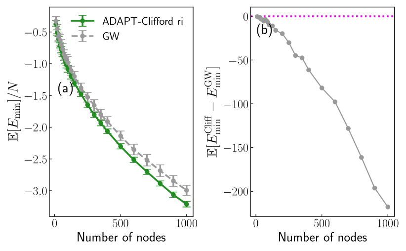
Figure 2: Performance of randomized ADAPT-Clifford on weighted complete graphs. (a) Normalized energy found by randomized ADAPT-Clifford (green circles) and GW (light grey circles) averaged over $100$ instances. (b) Instance averaged minimum energy difference between the solution found with randomized ADAPT-Clifford and GW as a function of problem size. Notice that randomized ADAPT-Clifford is almost always superior to GW. The magenta dotted line indicates a mean energy difference of zero. We have omitted the error bars for the sake of clarity.

The results of Sec. III indicate that the precise choice of positive weight distribution may be immaterial. We have verified numerically that this is indeed the case for a few different weight distributions. In this subsection, we focus the discussion to $\omega_{i,j}$ sampled from ${\rm U}[0,1]$ and leave an exhaustive investigation for future work.

We begin studying the performance of the randomized approach. We draw a parallel between the random initialization of ADAPT-Clifford and the rounding step of GW, and thus assess the performance of the randomized ADAPT-Clifford by direct comparison with GW. We solved $100$ different problem instances for graph sizes up to $N=1000$ with both algorithms. In Fig. 2a we show the normalized mean minimum energy, $\mathbb{E}[E_{\rm min}]/N$, of the solutions obtained with randomized ADAPT-Clifford (green circles) and the ones obtained with GW (light grey circles). Notice that our randomized ADAPT-Clifford almost always produces a solution of lower energy expectation than GW. These observations can be further verified with the mean difference of the minimum energy found, $\mathbb{E}[E_{\rm min}^{\rm Cliff}-E_{\rm min}^{\rm GW}]$, which we show in Fig. 2b. Since our randomized ADAPT-Clifford consistently beats GW, we expect it to have a performance guarantee for typical instances of positively weighted complete graphs above that of GW for the general problem. We discuss the methodology used to estimate it in App. D. We find $\overline{\alpha}^{\rm r}\approx 0.8986$ a value which confirms our intuition and sets a lower bound for the expected performance of the deterministic ADAPT-Clifford.

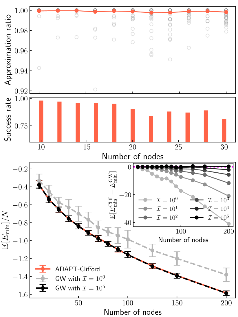
Figure 3: (a) Approximation rations $\alpha$ (empty circles) and mean approximation ratios (orange full circles) of solutions to MaxCut on $100$ weighted complete graphs per graph size found with deterministic ADAPT-Clifford. (b) Success rate on the $100$ problem instances per graph size considered in (a). (c) Instance-averaged minimum energy over $60$ problems up to graphs with $200$ nodes, both whit our algorithm (orange solid line), with Goemans-Williamson algorithm (light grey dashed line), and Goemans-Williamson with $\mathcal{I}=10^{5}$ (black dashed line). The inset shows the mean difference in the minimum energies found by our algorithm and the GW algorithm as a function of the problem size and for different values of $\mathcal{I}$. The magenta dotted line indicates a mean energy difference of zero. In the inset we have omitted the error bars for the sake of clarity.

We now focus on the deterministic approach. First, we benchmark this algorithm for instances with size up to $N=30$ for which the exact solution can be found exhaustively. Fig. 3a shows the exact approximation ratios $\alpha$, obtained for $100$ problem instances. For these small problems, our algorithm performs, on average, above $\alpha=0.997$, with the value of the minimum $\alpha$ increasing as $N\to 30$. We notice that the number of instances for which our algorithm finds the exact ground state slightly decreases with the problem size. The success rate, defined as the number of times the algorithm finds a cut with energy $E_{\rm min}^{\rm Cliff}-E^{\rm C}_{\rm min}<10^{-10}$, is shown in Fig. 3b as a function of the problem size. We observe a success rate $\sim 80\%$ for $N=30$.

For problem sizes beyond $N=30$, when we cannot access the exact value of the ground state energy, we resort to a direct comparison with the GW algorithm. We find that the cuts obtained with deterministic ADAPT-Clifford are of superior quality to those found with the standard GW algorithm. To obtain a comparison, we thus systematically increase the number of times $\mathcal{I}$ the rounding step is performed in GW and return the best cut found —see App. A for details. The standard GW algorithm thus corresponds to $\mathcal{I}=1$. In Fig. 3c we show the normalized mean energies $\mathbb{E}[E_{\rm min}]/N$ for $60$ problem instances up to a problem size of $N=200$ produced by our algorithm (orange circles), standard GW (light grey circles), and GW with $\mathcal{I}=10^{5}$ (black circles). Notice that our algorithm produces cuts which are always, not merely on average, better than those produced with standard GW, and only when we reach $\mathcal{I}=10^{5}$ does the GW algorithm begin to produce a cut whose quality is, on average, superior to that of the cut produced by our algorithm.

To further verify this observation, the inset of Fig. 3c shows the mean energy difference, $\mathbb{E}[E_{\rm min}^{\rm Cliff}-E_{\rm min}^{\rm GW}]$, between the solution found with our algorithm and the one found with GW, with the magenta dotted line indicating $\mathbb{E}[E_{\rm min}^{\rm Cliff}-E_{\rm min}^{\rm GW}]=0$, that is, equal quality cuts on average. It is seen that ADAPT-Clifford performs increasingly better than GW with fixed $\mathcal{I}$ as problem size is increased. To quantify the approximation quality of ADAPT-Clifford, we estimate the average approximation ratio of the deterministic ADAPT-Clifford on this family of graphs to be $\overline{\alpha}=0.9686$ – see App. D for details.

While Fig. 3c shows that $\mathcal{I}=10^{5}$ rounding steps are needed for the GW algorithm to match the approximation quality of the deterministic ADAPT-Clifford for problem sizes up to $N=200$, the data in the inset imply that $\mathcal{I}$ may in fact need to scale with $N$ for the GW algorithm to compete with ADAPT-Clifford. Therefore, although the expected runtime of standard GW $O(N^{3.5})$, see [30, 89] and references therein, compared to $O(N^{6})$ for ADAPT-Clifford on complete graphs, our benchmarks are inconclusive as to which of the two algorithms is faster.

V.2 Signed weights: the Sherrington-Kirkpatrick model

The Sherrington-Kirkpatrick (SK) model [90] has played a fundamental role in the advancement of the understanding of the physics of spin glasses and disordered systems [91, 92, 93, 94]. It describes $N$ classical spins with all-to-all couplings of both ferromagnetic and antiferromagnetic character. The Hamiltonian is given by

$$H_{\rm sk}=\frac{1}{\sqrt{N}}\sum_{i<j}\omega_{i,j}\sigma_{i}\sigma_{j},$$ (24)

where $\sigma_{i}\in\{-1,1\}$ is a classical spin and the couplings $\omega_{i,j}$ are sampled from a distribution with zero mean and unit variance, for instance the normal distribution $\mathcal{N}(0,1)$. A milestone result by Parisi [95, 96] gave an explicit expression for the ground state energy density of this model in the thermodynamic limit, which we refer to as the Parisi value,

$$\lim_{N\to\infty}\mathbb{E}\left[\frac{E^{\rm sk}_{\rm min}}{N}\right]=\Pi^{*}=-0.763166...,$$ (25)

where the expectation value is over realizations of the random couplings, and $E^{\rm sk}_{\rm min}$ refers to the ground state energy of Hamiltonian in Eq. (24). The most accurate numerical value of Eq. (25) to date was computed in Ref. [97]. The limit in the LHS of Eq. (25) has been formally shown to both exist and be equal to the Parisi value [98, 99].

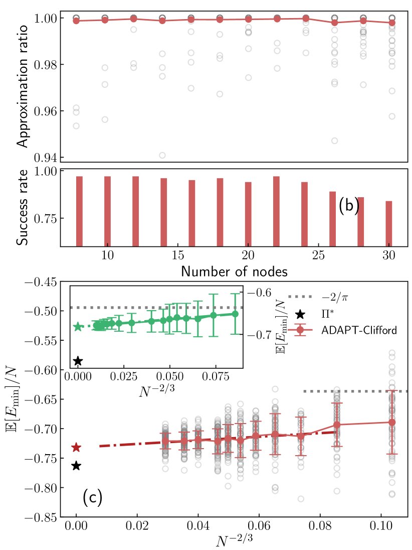
Figure 4: (a) Approximation rations $\alpha$ (empty circles) and mean approximation ratios (red full circles) of deterministic ADAPT-Clifford for $100$ different disorder realizations of the SK model per system size. (b) Success rate on the $100$ problem instances per graph size considered in (a). (c) Ground-state energy density for each of the $100$ problem instances (empty circles) per problem size up to $N=200$, and their mean (full circles). The dashed-dotted line show the best linear fit and the red star the respective mean energy density in the thermodynamic limit. The inset shows the average ground state energy density up to $N=1000$ as obtained with randomized ADAPT-Clifford, with its corresponding linear fit (see main text) and the value in the thermodynamic limit (green star). The grey dotted line shows the mean energy density obtained with semidefinite programing and the black star shows the Parisi value $\Pi^{*}$.

Recently the SK model has been used as a benchmark in the study of quantum approximate optimization algorithms [100, 101, 15]. Motivated by these works, we focus our attention on this model to characterize the performance of our algorithm on complete graphs with signed weights. A word of caution: The ADAPT-QAOA solution circuits for the signed case, including small instances of the SK model, are not completely Clifford, see Fig. 1b,d and Sec. III. As such, we do not expect our algorithm to match the solution quality of the best classical algorithm due to Montanari [102, 103], which produces a $\boldsymbol{\sigma}^{*}$ with energy below $(1-\epsilon)$ times the lowest energy for typical instances, with $\epsilon$ a small positive constant . Nevertheless, we are interested in seeing how close the $\boldsymbol{\sigma}^{*}$'s produced by our algorithm get to the Parisi value, both for the randomized and deterministic variants of ADAPT-Clifford.

In order to utilize ADAPT-Clifford we promote the classical spin in Eq. (24) to $\sigma_{i}\to Z_{i}$ and use the resulting Hamiltonian as our cost. Following the presentation of the previous subsection, we discuss first the performance of the randomized ADAPT-Clifford. The green circles in the inset of Fig. 4c show $\mathbb{E}\left[\frac{E_{\rm min}}{N}\right]$ for this algorithm with problem sizes up to $N=1000$. To obtain its value in the thermodynamic limit we fit the data for $N\in[40,1000]$ to a model of the form $qN^{-2/3}+\Pi^{\rm Cliff}_{\rm ri}$  where $\Pi^{\rm Cliff}_{\rm ri}$ corresponds to the mean energy density in the thermodynamic limit obtained with the randomized ADAPT-Clifford. We find $\Pi^{\rm Cliff}_{\rm ri}\approx-0.682$ which corresponds to $\sim 89\%$ of the Parisi value (black star in inset of Fig. 4c). This value is below what is obtained with convex relaxation methods, for instance semidefinite programming, which is known to give $\mathbb{E}\left[\frac{E_{\rm min}}{N}\right]=-\frac{2}{\pi}+o(1)\approx-0.6366$ with $o(1)$ a number which vanishes for $N\to\infty$ [106, 107]. For comparison we display $\mathbb{E}\left[\frac{E_{\rm min}}{N}\right]=-\frac{2}{\pi}$ as the horizontal dotted line both in the inset and in Fig. 4c.

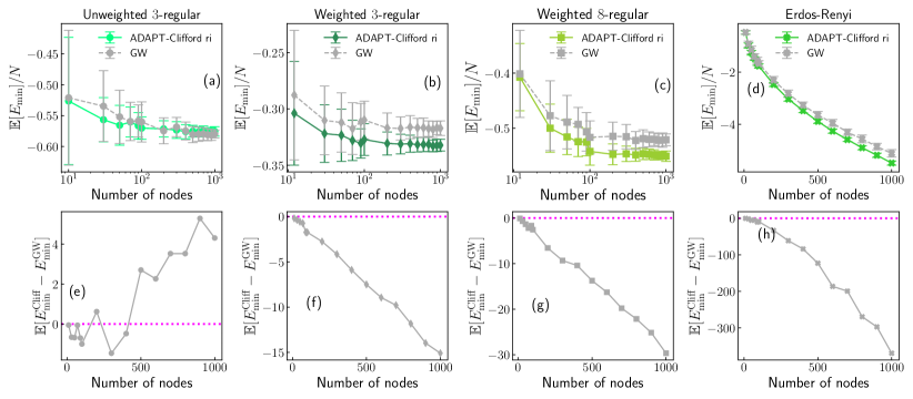
Figure 5: Performance of randomized ADAPT-Clifford vs GW. (a-d) Normalized instance-averaged minimum energy found with randomized ADAPT-Clifford (colorful markers and solid lines) and standard GW (light grey markers and dashed lines). The different graph types studied are: (a) unweighted $3$-regular graphs, (b) weighted $3$-regular graphs, (c) weighted $8$-regular graphs, (d) unweighted Erdös-Rényi graphs with edge probability $1/2$. For the weighted case we take $\omega_{i,j}$ in ${\rm U}[0,1]$. (e-h) Instance-averaged minimum energy differences between the solutions found with ADAPT-Clifford and standard GW for (e) unweighted $3$-regular (circles), (f) weighted $3$-regular (diamonds), (g) weighted $8$-regular (squares), and (h) Erdos-Renyi with edge probability $1/2$ (exes). The magenta dotted line indicates equal energy of the solutions found on average. We have omitted the error bars to avoid saturating the figure. All averages were computed over $100$ randomly generated instances.

Let us now consider the deterministic ADAPT-Clifford. For small problems $N\in[10,30]$ we computed the exact approximation ratios $\alpha$ over $100$ problem instances, and show them as empty circles in Fig. 4a. Notably we do not observe $\alpha<0.94$ for any instance, and the average over instances is always above $\alpha>0.997$. To complement this observation we compute the success rate, defined as the number of instances for which the difference $E^{\rm SK}_{\rm min}-E_{\rm min}^{\rm Cliff}<10^{-10}$. These are shown in Fig. 4b with the smallest one being $\sim 82\%$ at $N=30$.

To fully explore the performance of the deterministic ADAPT-Clifford algorithm, we solve $100$ instances for problems up to $N=200$. The normalized energies $E_{\rm min}^{\rm Cliff}/N$ are shown as empty circles in Fig. 4c for all the instances considered, the red full circles show the respective $\mathbb{E}[E_{\rm min}^{\rm Cliff}]/N$ and the error bars correspond to the standard deviation of the normalized energies. To assess the quality of the solutions found we consider the data in the interval $N\in[40,200]$ and fit it to a model of the form $qN^{-2/3}+\Pi^{\rm Cliff}$ with $\Pi^{\rm Cliff}$ the estimated mean energy density in the thermodynamic limit of the solutions found by our algorithm. In particular for $N=200$ we find $\mathbb{E}\left[\frac{E^{\rm Cliff}_{\rm min}}{N}\right]\approx-0.727...$ and from the linear fit we find $\Pi^{\rm Cliff}\approx-0.7409...$, shown by a red star in Fig. 4c. These values correspond to $\sim 94\%$ and $\sim 97\%$ of the Parisi value, respectively (the latter is shown with a black star in Fig. 4c). These values are below what is obtained with convex relaxation methods (horizontal dotted line in Fig. 4c). Notably, the value reached by our algorithm for $N=200$ is already better than what can be obtained with zero-temperature simulated annealing which gives $\mathbb{E}\left[\frac{E_{\rm min}}{N}\right]\sim-0.71$ (as quoted in Ref. [100]), and $\Pi^{\rm Cliff}$ is comparable to what is achievable with simulated annealing on large problem instances.

VI Algorithm performance on other families of graphs

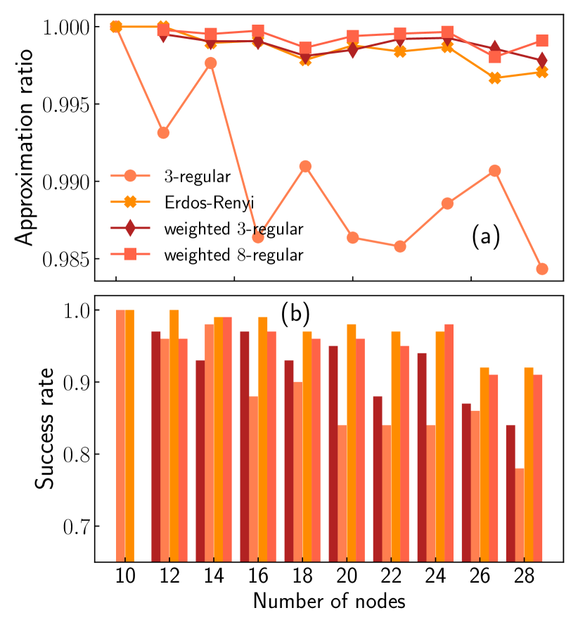
Figure 6: (a) Instance averaged approximation ratios up to $N=28$ for $100$ different instances of: unweighted $3$-regular graphs (circles), weighted $3$- (diamonds) and $8$-regular graphs (squares) with $\omega_{i,j}\in{\rm U}[0,1]$, and Erdös-Rényi graphs with edge probability $1/2$ (exes). We have omitted the error bars for clarity. (b) Success rate for each of the problem sizes and graph types considered in (a).

In this section, we characterize the performance of ADAPT-Clifford in both its variants for the MaxCut problem on $K$-regular graphs (unweighetd and weighted) and unweighted Erdos-Renyi graphs with various edge probabilities. For the randomized ADAPT-Clifford, we directly compare the quality of the cuts found with standard GW, while for determinisitic ADAPT-Clifford we discuss the exact approximation ratios for small problems and compare against GW with variable $\mathcal{I}$, the number of time the rounding step is performed.

VI.1 Performance on $K$-regular graphs

We consider $3$-regular and $8$-regular graphs, unweighted and weighted. In all cases edge weights are sampled from ${\rm U}[0,1]$.

In Fig. 5a-c we show the normalized instance-averaged minimum energy of the solutions found with randomized ADAPT-Clifford and standard GW. For large ($N>200$) unweighted $3$-regular graphs, GW finds better solutions, on average, than randomized ADAPT-Clifford —see Fig. 5e. The situation is markedly reversed with the inclusion of nontrivial edge weights, with randomized ADAPT-Clifford outperforming standard GW (see Fig. 5b), and the performance margin widens with increased connectivity, see Fig. 5c. These observations are verified with the averaged minimum energy differences shown in Fig. 5f,g for weighted $3$- and $8$-regular graphs, respectively. Thus, GW performs better than randomized ADAPT-Clifford only for unweighted $3$-regular graphs, while the comparative performance of our algorithm consistently improves with both the inclusion of edge weights and higher connectivity.

We now move to the performance of deterministic ADAPT-Clifford. In Fig. 6a we show the mean approximation ratios over $100$ problem instances for each of these types of graphs. For the unweighted $3$-regular graphs we consider problem sizes $N\in[10,28]$ and for the weighted problems we consider problem sizes $N\in[12,28]$. We have omitted the error bars from the figure for the sake of clarity. Deterministic ADAPT-Clifford shows the poorest performance for unweighted $3$-regular graphs, circles in Fig. 6a, with a decreasing mean $\alpha$ as $N$ increases. Interestingly the comparative performance of ADAPT-Clifford improves upon inclusion of edge weights, diamonds in Fig. 6a, with a mean $\alpha$ above $0.995$ for all problem sizes considered. Further improved performance is observed with higher edge connectivity, as evidence by the mean approximation ratio for weighted $8$-regular graphs (squares in Fig. 6a). In Fig. 6b we show the success rate of the algorithm, i.e., the number of times ADAPT-Clifford found the maximal cut. The $3$-regular graphs (unweighted and weighted) show a success rate which consistently decay with problem size. On the contrary for weighted $8$-regular graphs our algorithm shows a success rate above $90\%$ up to $N=28$.

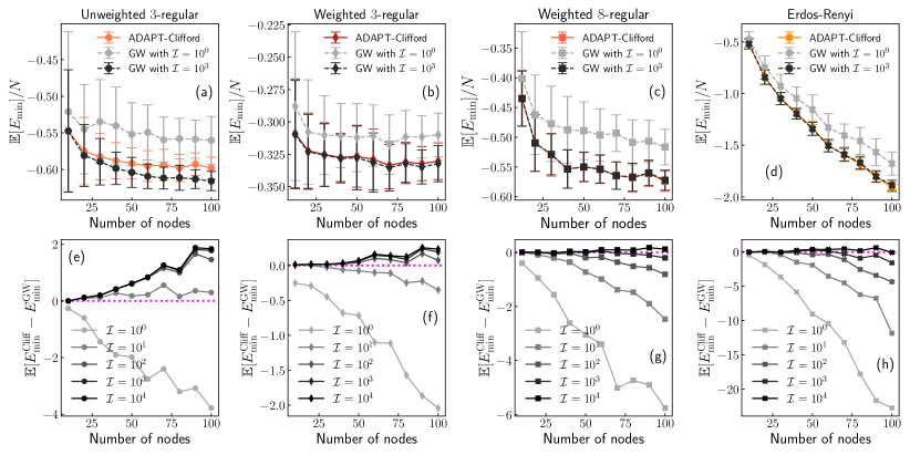
Figure 7: (a-d) Normalized instance-averaged minimum energy found over $100$ instances for problem sizes up to $N=100$ and different graph types obtained with deterministic ADAPT-Clifford (colorful markers and solid lines), with standard GW (light grey markers and dashed lines), and GW with $\mathcal{I}=10^{3}$ (dark grey markers and dashed lines). The different graph types studied are: (a) unweighted $3$-regular graphs, (b) weighted $3$-regular graphs, (c) weighted $8$-regular graphs, (d) unweighted Erdös-Rényi graphs with edge probability $1/2$. For the weighted case we always take $\omega_{i,j}$ in ${\rm U}[0,1]$. (e-h) Instance averaged minimum energy differences between the solutions found with our algorithm and the solution found with GW with different values of $\mathcal{I}$. For the graph types: (e) unweighted $3$-regular (circles), (f) weighted $3$-regular (diamonds), (g) weighted $8$-regular (squares), and (h) Erdos-Renyi with edge probability $1/2$ (exes). As a reference the the magenta dotted line indicates equal energy of the solutions found on average. We have omitted the error bars to avoid saturating the figure.

For larger problem sizes, we compare the solution quality of deterministic ADAPT-Clifford with that of GW with variable $\mathcal{I}$ ($\mathcal{I}=1$ is the standard GW algorithm). Fig. 7a,b,c shows the normalized mean minimum energy $\mathbb{E}[E_{\rm min}]/N$ for the $K$-regular graphs studied. Notably, deterministic ADAPT-Clifford produces solutions of lower energy than GW for all three graph ensembles under consideration, compare the colorful markers with the light grey markers in Fig. 7a,b,c. For the unweighted $3$-regular graphs, Fig. 7a, already at $\mathcal{I}=10$ GW consistently finds a cut of lower energy than deterministic ADAPT-Clifford, signaling at a reduced performance of the latter method compared to the case of weighted complete graphs. This observation can be further verified with the mean difference of the minimum energy found, $\mathbb{E}[E_{\rm min}^{\rm Cliff}-E_{\rm min}^{\rm GW}]$, shown in Fig. 7e.

Similarly to its randomized counterpart, deterministic ADAPT-Clifford performs more competitively when edge weights are included. In Fig. 7b we show the $\mathbb{E}[E_{\rm min}]/N$ obtained with our algorithm (red diamonds), GW (light grey diamonds), and GW with $\mathcal{I}=10^{3}$ (black diamonds), for the weighted $3$-regular graphs. Further inspection of the corresponding $\mathbb{E}[E_{\rm min}^{\rm Cliff}-E_{\rm min}^{\rm GW}]$, shown in Fig. 7f, shows that at least $\mathcal{I}=10^{2}$ are necessary for the GW solution to be, on average, superior to that found by our algorithm. The performance margin widens as we move to regular graphs with higher connectivity. Fig. 7c shows $\mathbb{E}[E_{\rm min}]/N$ obtained with deterministic ADAPT-Clifford (orange squares), standard GW (light grey squares), and GW with $\mathcal{I}=10^{3}$ (black squares), for weighted $8$-regular graphs. After inspecting the $\mathbb{E}[E_{\rm min}^{\rm Cliff}-E_{\rm min}^{\rm GW}]$ in Fig. 7g we observe that $\mathcal{I}=10^{4}$ is necessary for the GW solution to be consistently better than the deterministic ADAPT-Clifford solution. Thus, for sparse graphs the performance of both randomized and deterministic ADAPT-Clifford improves with the inclusion of edge weights and/or higher node connectivity.

VI.2 Performance on unweighted Erdös-Rényi graphs

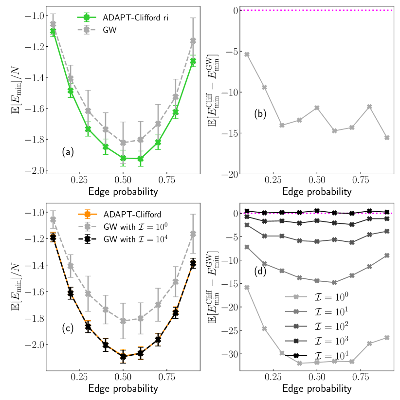
Figure 8: (a) Normalized instance-averaged minimum energy of the solutions found with randomized ADAPT-Clifford (green) and GW (light grey). (b) Instance averaged minimum energy differences between the solutions found with our algorithm and the solution found with GW. (c) Normalized instance averaged minimum energy of the solutions found with the deterministic ADAPT-Clifford (orange), standard GW (light grey), and GW with $\mathcal{I}=10^{4}$ (black), as a function of the edge probability which we take in $[0.1,0.9]$. (d) Instance averaged minimum energy differences between the solutions found with our algorithm and the solution found with GW with different values of $\mathcal{I}$, as a function of edge probability. The magenta dotted line indicates mean energy difference of zero. The averages are taken over $100$ different problem instances and for $N=120$.

We now wish to characterize the performance of ADAPT-Clifford for MaxCut on dense graphs with variable density. For this task we will focus on unweighted Erdös-Rényi graphs.

First, we fixed the edge probability to $1/2$ and study the performance with respect to the problem size. In Fig. 5e we show the instance averaged minimum energy of solutions obtained with randomized ADAPT-Clifford (green) and standard GW (light grey). For graphs up to $N=1000$. The randomized version of our algorithm produces better solutions, on average, than GW, an observation that is verified by the instance-averaged minimum energy differences shown in Fig. 5h.

Next, we analyze the performance of the deterministic ADAPT-Clifford on small problems $N\leq 28$. Fig. 6a,b show mean approximation ratios (exes), which is above $\alpha\sim 0.997$, and success rates, respectively. Notably, deterministic ADAPT-Clifford shows a higher success rate for this family of graphs, finding the maximal cut on all instances considered for the sizes $N=10,12$ (whereas it only achieves the same for the $19$ nonisomorphic $3$-regular graphs at $N=10$). For larger problems, in Fig. 7d we compare the normalized instance-averaged minimum energy found by our algorithm (orange solid line), standard GW (light grey dashed line), and GW with $\mathcal{I}=10^{3}$ (black dashed line). Our algorithm (orange) finds a solution of lower energy, on average, than that found with GW (light grey). We explore the extent of this advantage by inspecting the mean difference of the minimum energy found, $\mathbb{E}[E_{\rm min}^{\rm Cliff}-E_{\rm min}^{\rm GW}]$, as a function of $N$ and with $\mathcal{I}$ as a control parameter. The results are shown in Fig. 7h. It is seen that only at $\mathcal{I}=10^{4}$ the GW solutions are consistently of lower energy than those found by deterministic ADAPT-Clifford.

Now we turn our attention to benchmarking both the randomized and deterministic ADAPT-Clifford on Erdös-Rényi graphs with varying edge inclusion probability. We focus on problems with $N=120$ and consider edge probabilities in $[0.1,0.9]$. We solve $100$ problem instances of MaxCut per edge inclusion probability. In Fig. 8a we show the normalized mean energies found with the randomized ADAPT-Clifford (green) and with standard GW (light grey). Our randomized algorithm returns, on average, a cut of better quality than GW (see also instance-averaged minimum energy differences in Fig. 8b). The normalized mean energies of the solutions found with deterministic ADAPT-Clifford (orange) are shown in Fig. 8c, alongside those for standard GW (light grey), and GW with $\mathcal{I}=10^{4}$ (black). With the exception of edge probabilities smaller than $0.15$ and larger than $0.85$, the solutions found by our algorithm are always, not merely on average, better than the ones found with GW, with the largest advantage observed for edge probabilities around $1/2$. Only at $\mathcal{I}\sim 10^{4}$ does GW produce solutions on average comparable to those found by ADAPT-Clifford. This is seen more clearly in the instance-averaged energy difference of the solutions found $\mathbb{E}[E_{\rm min}^{\rm Cliff}-E_{\rm min}^{\rm GW}]$, shown in Fig. 8b. Only at $\mathcal{I}=10^{4}$ we find $\mathbb{E}[E_{\rm min}^{\rm Cliff}-E_{\rm min}^{\rm GW}]\in(0,0.5]$ for all edge probabilities, indicating our algorithm no longer offers an advantage over GW.

The results discussed here suggest that ADAPT-Clifford offers an advantage over GW on the quality of the cut found for dense graphs, with the largest gap for graphs with density $\sim 1/2$.

VII Discussion and outlook

We introduce ADAPT-Clifford, a quantum inspired classical approximation algorithm for MaxCut. For each problem instance, ADAPT-Clifford builds a low-depth Clifford circuit to prepare a stabilizer state that encodes an approximate solution. The algorithm was inspired by observation of the (almost) Clifford character of the ADAPT-QAOA solution circuits for MaxCut on weighted fully connected graphs. We introduce a randomized and a deterministic variant of this algorithm. Their respective runtime complexities are $O(N^{4})$ and $O(N^{5})$ for sparse graphs, and $O(N^{5})$ and $O(N^{6})$ for dense graphs, and in all cases the space complexity is $O(N^{2})$. Naturally, the deterministic variant always outperforms the randomized variant, albeit at the cost of an increased runtime.

We have studied the performance of ADAPT-Clifford on MaxCut for various families of graphs, both dense and sparse, and both unweighted and weighted. On weighted complete graphs with positive weights, ADAPT-Clifford finds very high quality cuts, reaching the absolute maximum in the majority of small instances. Moreover, the algorithm is scalable, allowing us to easily find solutions for instances with up to $1000$ nodes. ADAPT-Clifford also performs well for signed weights, finding good approximations to the ground state of the SK model with an energy that extrapolates to $97\%$ of the Parisi value in the thermodynamic limit. To investigate performance as a function of density, we applied ADAPT-Clifford to MaxCut on unweighted Erdös-Rény graphs with variable edge inclusion probability. We again find that ADAPT-Clifford finds the absolute maximum cut for the majority of small instances and easily scales to hundreds of nodes. Finally, we study the performance of ADAPT-Clifford for sparse graphs. Even though these graphs are far from the context that gave rise to the algorithm, we find that ADAPT-Clifford still performs well, producing the absolute maximum cut with high probability for small instances and easily scaling to $1000$ nodes. Only for the case of $3$-regular graphs, the sparsest category of graphs we studied, we observe a noticeable deterioration in solution quality with increasing size. Counter-intuitively, performance improves somewhat with the inclusion of edge weights.

To assess the performance of ADAPT-Clifford for large problem instances whose exact solution is intractable, we compare its performance with the GW algorithm, which represents the state of the art in approximate solution of MaxCut. For all graph families studied, ADAPT-Clifford outperforms the standard GW algorithm in the quality of the cut found. Only for very sparse unweighted graphs, such as $3$-regular graphs, the performance of the GW algorithm becomes comparable to that of ADAPT-Clifford, but even in this case the inclusion of edge weights favors the latter. Finally, ADAPT-Clifford solves problems to which the GW algorithm is not directly applicable, as exemplified by our results on the SK model.

The Clifford or near Clifford character of the ADAPT-QAOA solution circuits is a key observation which was missed in previous work [108]. This observation, as laid out in Sec. III, allowed us to devise a quantum-inspired, polynomial-time approximartion algorithm for MaxCut. While it is known that MaxCut on dense graphs admits Polynomial Time Approximation Schemes (PTAS), leading to approximated solutions which are $1-\epsilon$ away from the optimum in time polynomial in $N$ [50, 51], the scaling of the runtime as a function of $\epsilon$ may render these algorithms impractical. In contrast, in this work we showed empirically that ADAPT-Clifford performs better than an algorithm that offers a guaranteed approximation ratio.

We hope the results reported here will help delimit the subset of graphs where a quantum speedup could be expected and thus where the current efforts should focus, in similar spirit to previous results obtained with a different subuniversal family of gates [109]. While our work indicates that ADAPT-Clifford has a guaranteed approximation ratio, we do not yet have a proof. Whether it is possible to improve the runtime without compromising the solution quality is also an open problem. Our algorithm showed the poorest performance on fully connected graphs with signed weights. This was anticipated in Sec. III since the ADAPT-QAOA solution circuits are not fully Clifford. However, they are near-Clifford, motivating then a resource-centered design of variational ansätze, with a Clifford mixer part constructed following a scheme like the one introduced in this work, similar in spirit to the optimal mixers restricted to subspaces [110], and a cost part with few variational parameters adding just the right amount of nonCliffordness necessary to approximate the problem up to a desired ratio. Furthermore our algorithm could aid in reducing the cost of parameter optimization in QAOA when used to warm-start [111] it. Finally, our Clifford algorithm was tailored to solve the MaxCut problem. It remains an open question to what extent other combinatorial optimization problems admit Clifford approximation algorithms with practical polynomial runtimes.

Appendix A The Goemans-Williamson algorithm

Suppose we are interested in solving the MaxCut problem for some given graph $\mathcal{G}=(\mathcal{V},\mathcal{E})$ of $N$ nodes and edge weights $\omega_{i,j}$ using the Goemans-Williamson algorithm [30, 31]. To do so one proceeds as follows:

1. Relax the binary character of the variables in the optimization problem defined by the cost function in Eq. (1), that is, replace the $z_{i}\in\{0,1\}$ with unit vectors $y_{i}\in\mathbb{R}^{N}$ and the product $z_{i}z_{j}$ with the inner product $y_{i}^{T}y_{j}$ with $T$ the transpose. The new cost function $\sum_{i,j<i}\omega_{i,j}(1-y_{i}^{T}y_{j})$ with the constraints $y_{i}^{T}y_{i}=1$, $\tilde{Y}=[y_{i}^{T}y_{j}]$ is positive semidefinite, defines a semidefinite program.

2. Solve the semidefinite program using a polynomial time algorithm, and find an optimal solution $\tilde{Y}^{*}$ for the relaxed problem.

3. Rounding. Choose a random vector $\mathbf{r}\in\mathbb{R}^{N}$ from a Gaussian distribution and for all $i$ define $h_{i}={\rm sgn}(\mathbf{r}^{T}y^{*}_{i})$, where ${\rm sgn}(x)$ is the sign function. This assignment defines a partition of the nodes in two disjoint sets $\mathcal{A}=\{i|h_{i}=1\}$ and $\overline{\mathcal{A}}=\{i|h_{i}=-1\}$.

4. return the cut $(\mathcal{A},\overline{\mathcal{A}})$.

In this form the algorithm only performs the rounding, step (3), a single time based on a single random vector $\mathbf{r}$. As such, a simple improvement consists on repeating this step $\mathcal{I}$ times for different random vectors and then returning the cut of largest cost among all the cuts found. We have used this approach in comparing our algorithm with GW.

All the results for the GW algorithm reported in this manuscript have been obtained using a freely available Julia implementation .

Appendix B Validity of the search through a restricted set of pairs

In step (2) of ADAPT-Clifford in Sec. IV, we restricted our search to pairs of the form $(\tilde{l},b^{(r-1)})$ with $\tilde{l}\in\{k,j\}$ and $(k,j)$ is the edge where the first two-qubit gate was applied, and $b^{(r-1)}\in\mathbf{b}^{(r-1)}$. In this appendix we show than in doing so we do not miss the value of the largest gradient.

At step $r>1$ the gradient is of the form

$$g_{a^{(r-1)},b^{(r-1)}}^{(r)}=-\sum_{l}\omega_{l,b^{(r-1)}}\langle Z_{l}X_{b^{(r-1)}}Z_{a^{(r-1)}}\rangle_{r-1}\\ =-\sum_{l}\omega_{l,b^{(r-1)}}\langle Z_{l}Z_{a^{(r-1)}}\rangle_{r-1},$$ (26)

where we have used the fact that $X_{b^{(r-1)}}|\psi_{r-1}\rangle=|\psi_{r-1}\rangle$ since $b^{(r-1)}$ is inactive. The maximum of Eq. (26) happens at the pair $(a^{(r-1)},b^{(r-1)})$ such that the number of $l$'s, with $l\in\mathbf{a}^{(r-1)}$, for which $-Z_{l}Z_{a^{(r-1)}}|\psi_{r-1}\rangle=|\psi_{r-1}\rangle$ is the largest.

Now consider the situation of interest where we search for the pair to apply the gate among those of the form $(\tilde{l},b^{(r-1)})$, and suppose we know that the maximum of Eq. (26) occurs at the pair $(\tilde{a},\tilde{b})$ with $\tilde{a}\in\mathbf{a}^{(r-1)}$ and $\tilde{b}\in\mathbf{b}^{(r-1)}$. Then

$$g_{\tilde{a},\tilde{b}}^{(r)}=\sum_{l}\omega_{l,\tilde{b}}\langle-Z_{l}Z_{\tilde{a}}\rangle_{r-1}\\ =\sum_{l}\omega_{l,\tilde{b}}\langle-Z_{l}Z_{\tilde{l}}Z_{\tilde{l}}Z_{\tilde{a}}\rangle_{r-1},$$ (27)

where we introduced an identity $\mathbb{I}_{\tilde{l}}=Z_{\tilde{l}}Z_{\tilde{l}}$.

Since $\tilde{a}$ is active and $-Z_{k}Z_{j}|\psi_{r-1}\rangle=|\psi_{r-1}\rangle$ we can always pick the value of $\tilde{l}\in\{k,j\}$ such that $Z_{\tilde{a}}Z_{\tilde{l}}|\psi_{r-1}\rangle=|\psi_{r-1}\rangle$. Thus, we can extend Eq. (27) to the following chain of equalities

$$g_{\tilde{a},\tilde{b}}^{(r)}=\sum_{l}\omega_{l,\tilde{b}}\langle-Z_{l}Z_{\tilde{l}}Z_{\tilde{l}}Z_{\tilde{a}}\rangle_{r-1}\\ =\sum_{l}\omega_{l,\tilde{b}}\langle-Z_{l}Z_{\tilde{l}}\rangle_{r-1}=g_{\tilde{l},\tilde{b}}^{(r)}.$$ (28)

We see then that the largest gradient does live within the restricted set of pairs of the form $(\tilde{l},b^{(r-1)})$.

Appendix C Some explicit examples of ADAPT-Clifford solving MaxCut

In this appendix, we go over the full analytical calculation of the steps involved in solving MaxCut using the algorithm introduced in Sec. IV for two small graphs with $N=4,5$ nodes. In order to keep the expressions clean we have decided to focus on the case of unweighted graphs.

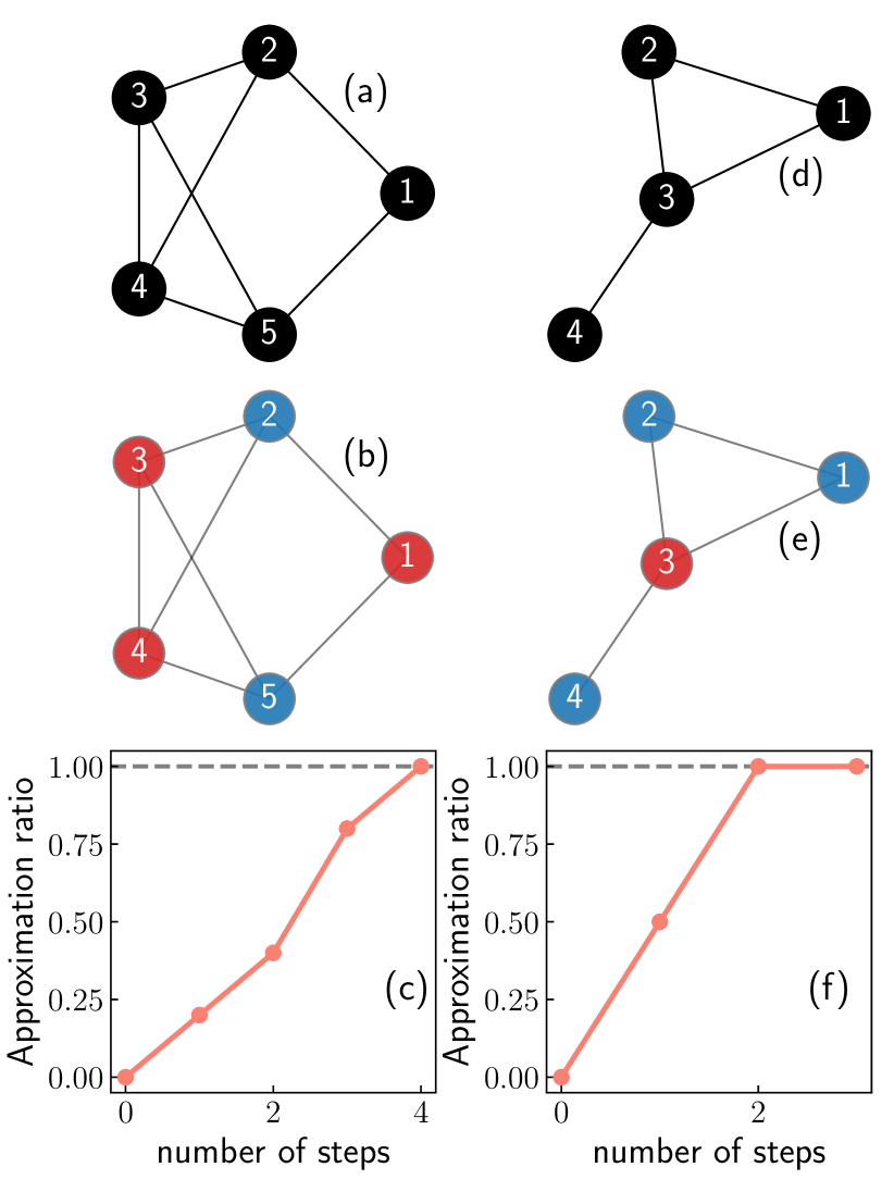
Figure 9: (a,d) Example graphs with $N=5$ and $N=4$ nodes, respectively. (b,e) Partitioned graphs according to the cuts produced by our algorithm, different colors denote the nodes in each of the disjoint subsets. (c,f) Approximation ratios of the states produced by our algorithm in the search process for the maximal cut of the graphs shown in (a) and (d). In both cases the algorithm reaches approximation ratio of $1$, indicating a maximal cut has been found.

C.1 An example with $N=5$ nodes

Consider the unweighted graph with five nodes shown in Fig. 9a. Its adjacency matrix is given by

$$[\omega_{i,j}]=\begin{pmatrix}0&&1&&0&&0&&1\\ 1&&0&&1&&1&&0\\ 0&&1&&0&&1&&1\\ 0&&1&&1&&0&&1\\ 1&&0&&1&&1&&0\end{pmatrix}.$$ (29)

We will solve MaxCut on this graph using our algorithm. We begin by flipping the state of the qubit at $k=2$, thus we have

$$|\psi_{0}\rangle=|+-+++\rangle,$$ (30)

where $|+\rangle=\mathrm{H}|0\rangle$ and $|-\rangle=Z\mathrm{H}|0\rangle$ are the eigenstates of the Pauli-$x$ operator corresponding to eigenvalues $+1$ and $-1$, respectively. At this point we have to initialize the records of active and innactive qubits, which we identify by their respective indices. The active qubits are $[2]$ and the inactive qubits are $[1,3,4,5]$.

Given our choice of initial position, we have that $g_{1,2}^{(1)}=g_{2,3}^{(1)}=g_{2,4}^{(1)}=1$ and are the largest “gradients”. We break this tie arbitrarily and chose the pair of qubits $(2,4)$. Then

$$|\psi_{1}\rangle=e^{i\frac{\pi}{4}Y_{2}Z_{4}}|\psi_{0}\rangle=\frac{1}{\sqrt{2}}\left[|+-+++\rangle-|+++-+\rangle\right],$$ (31)

and the records of the active and inactive qubits are updated to be $[2,4]$ and $[1,3,5]$, respectively. The second set of gradients is given by

$$g_{1,2}^{(2)} =-\sum_{l=2,5}\langle Z_{l}X_{1}Z_{2}\rangle=-\langle X_{1}\rangle-\langle Z_{5}X_{1}Z_{2}\rangle=-1+0=-1,$$ (32a)

$$g_{3,2}^{(2)} =-\sum_{l=2,4,5}\langle Z_{l}X_{3}Z_{2}\rangle=-\langle X_{3}\rangle-\langle Z_{4}X_{3}Z_{2}\rangle-\langle Z_{5}X_{3}Z_{2}\rangle=-1+1+0=0,$$ (32b)

$$g_{5,2}^{(2)} =-\sum_{l=1,3,4}\langle Z_{l}X_{5}Z_{2}\rangle=-\langle Z_{1}X_{5}Z_{2}\rangle-\langle Z_{3}X_{5}Z_{2}\rangle-\langle Z_{4}X_{5}Z_{2}\rangle=0+0+1=1,$$ (32c)

$$g_{1,4}^{(2)} =-\sum_{l=2,5}\langle Z_{l}X_{1}Z_{4}\rangle=-\langle Z_{2}X_{1}Z_{4}\rangle-\langle Z_{5}X_{1}Z_{4}\rangle=1+0=1,$$ (32d)

$$g_{3,4}^{(2)} =-\sum_{l=2,4,5}\langle Z_{l}X_{3}Z_{4}\rangle=-\langle Z_{2}X_{3}Z_{4}\rangle-\langle X_{3}\rangle-\langle Z_{5}X_{3}Z_{4}\rangle=1-1+0=0,$$ (32e)

$$g_{5,4}^{(2)} =-\sum_{l=1,3,4}\rangle Z_{l}X_{5}Z_{4}\rangle=-\langle Z_{1}X_{5}Z_{4}\rangle-\langle Z_{3}X_{5}Z_{4}\rangle-\langle X_{5}\rangle=-1,$$ (32f)

the largest gradients are $g_{5,2}^{(2)}$ and $g_{1,4}^{(2)}$. Since they are equal, we break the tie arbitrarily and chose the pair of qubits $(1,4)$. Thus the state at step $r=2$ is given by

$$|\psi_{2}\rangle=e^{i\frac{\pi}{4}Y_{1}Z_{4}}|\psi_{1}\rangle=\frac{1}{2}\left[|+-+++\rangle+|--+-+\rangle\right.\\ -\left.|+++-+\rangle-|-++++\rangle\right].$$ (33)

After the application of the gate we update the records of active and inactive qubits, which now are $[1,2,4]$ and $[3,5]$, respectively. The third set of gradients is given by

$$g_{3,1}^{(3)} =-\sum_{l=2,4,5}\langle Z_{l}X_{3}Z_{1}\rangle=-\langle Z_{2}X_{3}Z_{1}\rangle-\langle Z_{4}X_{3}Z_{1}\rangle-\langle Z_{5}X_{3}Z_{1}\rangle=1-1+0=0,$$ (34a)

$$g_{5,1}^{(3)} =-\sum_{l=1,3,4}\langle Z_{l}X_{5}Z_{1}\rangle=-\langle X_{5}\langle-\langle Z_{3}X_{5}Z_{1}\rangle-\langle Z_{4}X_{5}Z_{1}\rangle=-1+0-1=-2,$$ (34b)

$$g_{3,2}^{(3)} =-\sum_{l=2,4,5}\langle Z_{l}X_{3}Z_{2}\rangle=-\langle X_{3}\rangle-\langle Z_{4}X_{3}Z_{2}\rangle-\langle Z_{5}X_{3}Z_{2}\rangle=-1+1+0=0,$$ (34c)

$$g_{5,2}^{(3)} =-\sum_{l=1,3,4}\langle Z_{l}X_{5}Z_{2}\rangle=-\langle Z_{1}X_{5}Z_{2}\rangle-\langle Z_{3}X_{5}Z_{2}\rangle-\langle Z_{4}X_{5}Z_{2}\rangle=1+0+1=2,$$ (34d)

$$g_{3,4}^{(3)} =-\sum_{l=2,4,5}\langle Z_{l}X_{3}Z_{4}\rangle=-\langle Z_{2}X_{3}Z_{4}\rangle-\langle X_{3}\rangle-\langle Z_{5}X_{3}Z_{4}\rangle=1-1+0=0,$$ (34e)

$$g_{5,4}^{(3)} =-\sum_{l=1,3,4}\langle Z_{lX_{5}Z_{4}}\rangle=-\langle Z_{1}X_{5}Z_{4}\rangle-\langle Z_{3}X_{5}Z_{4}\rangle-\langle X_{5}\rangle=-1+0-1=-2.$$ (34f)

The largest gradient is $g_{5,2}^{(3)}=2$, the gate is applied at the pair of qubits $(2,5)$, where $2$ is an active qubit and $5$ is inactive. The state at step $r=3$ is given by

$$|\psi_{3}\rangle=e^{i\frac{\pi}{4}Z_{2}Y_{5}}|\psi_{2}\rangle=\frac{1}{2\sqrt{2}}\left[|+-+++\rangle+|++++-\rangle+|--+-+\rangle+|-++--\rangle\right.\\ \left.-|+++-+\rangle-|+-+--\rangle-|-++++\rangle-|--++-\rangle\right],$$ (35)

with the records of active and inactive qubits updated to $[1,2,4,5]$ and $[3]$, respectively. From this state we can compute the set of gradients of step $r=4$. They are given by

$$g_{1,3}^{(4)} =-\sum_{l=2,4,5}\langle Z_{l}X_{3}Z_{1}\rangle=-\langle Z_{2}X_{3}Z_{1}\rangle-\langle Z_{4}X_{3}Z_{1}\rangle-\langle Z_{5}X_{3}Z_{1}\rangle=1-1+1=1,$$ (36a)

$$g_{2,3}^{(4)} =-\sum_{l=2,4,5}\langle Z_{l}X_{3}Z_{2}\rangle=-\langle X_{3}\rangle-\langle Z_{4}X_{3}Z_{2}\rangle-\langle Z_{5}X_{3}Z_{2}\rangle=-1+1-1=-1,$$ (36b)

$$g_{4,3}^{(4)} =-\sum_{l=2,4,5}\langle Z_{l}X_{3}Z_{4}\rangle=-\langle Z_{2}X_{3}Z_{4}\rangle-\langle X_{3}\rangle-\langle Z_{5}X_{3}Z_{4}\rangle=+1-1+1=1,$$ (36c)

$$g_{5,3}^{(4)} =-\sum_{l=2,4,5}\langle Z_{l}X_{3}Z_{5}\rangle=-\langle Z_{2}X_{3}Z_{5}\rangle-\langle Z_{4}X_{3}Z_{5}\rangle-\langle X_{3}\rangle=-1+1-1=-1.$$ (36d)

There are two largest gradients, $g_{1,3}^{(4)}=g_{4,3}^{(4)}=1$. We break the tie arbitrarily and take the pair of qubits $(3,4)$. Thus the state at step $r=4$ is given by

$$|\psi_{4}\rangle=e^{i\frac{\pi}{4}Y_{3}Z_{4}}|\psi_{3}\rangle=\frac{1}{4}\left[|+-+++\rangle+|+---+\rangle+|++++-\rangle+|++---\rangle+|--+-+\rangle\right.\\ +|---++\rangle+|-++--\rangle+|-+-+-\rangle-|+++-+\rangle-|++-++\rangle-|+-+--\rangle\\ \left.-|+--+-\rangle-|-++++\rangle-|-+--+\rangle-|--++-\rangle-|-----\rangle\right].$$ (37)

To extract the cut found by our algorithm we should write $|\psi_{4}\rangle$ in the computational basis. In order to do this we use its stabilizers, which are

$$-XXXXX,\enspace-Z\mathbb{I}\mathbb{I}\mathbb{I}Z,\enspace+\mathbb{I}Z\mathbb{I}\mathbb{I}Z,\enspace-\mathbb{I}\mathbb{I}Z\mathbb{I}Z,\enspace-\mathbb{I}\mathbb{I}\mathbb{I}ZZ,$$ (38)

which correspond to the state

$$|\psi_{4}\rangle=\frac{1}{\sqrt{2}}\left(|10110\rangle-|01001\rangle\right),$$ (39)

in the computational basis. This state upon a measurement in this basis returns the cut $(\mathcal{A},\overline{\mathcal{A}})=([1,3,4],[2,5])$, which is a maximal cut of the graph under consideration. We illustrate this partitioning of the graph by coloring the nodes in $\mathcal{A}$ red and those in $\overline{\mathcal{A}}$ blue, and show the resulting partitioned graph in Fig. 9b. Additionally in Fig. 9c we show the approximation ratio of the states $|\psi_{r}\rangle$ computed in this section, notice that at $r=4$ we have approximation ratio equal to $1$, indicating the algorithm found a state compose of strings encoding maximal cuts.

C.2 An example with $N=4$ nodes

We consider now the graph with $N=4$ nodes shown in Fig. 9d. Its adjacency matrix is given by

$$[\omega_{i,j}]=\begin{pmatrix}0&&1&&1&&0\\ 1&&0&&1&&0\\ 1&&1&&0&&1\\ 0&&0&&1&&0\end{pmatrix}.$$ (40)

Let us start the algorithm wiht the state $|\psi_{0}\rangle=|+-++\rangle$. For this state there are two largest gradients at step $r=1$ given by $g_{2,3}^{(1)}=g_{2,1}^{(1)}=1$. We break the tie arbitrarily and pick the pair of qubits $(2,3)$. Thus the state at step $r=1$ is given by

$$|\psi_{1}\rangle=e^{i\frac{\pi}{4}Y_{2}Z_{3}}|\psi_{0}\rangle=\frac{1}{\sqrt{2}}\left[|+-++\rangle-|++-+\rangle\right].$$ (41)

Now, the gradients at step $r=2$ are given by

$$g_{1,2}^{(2)} =-\sum_{l=2,3}\langle Z_{l}X_{1}Z_{2}\rangle=-\langle X_{1}\rangle-\langle Z_{3}X_{1}Z_{2}\rangle=-1+1=0,$$ (42a)

$$g_{1,3}^{(2)} =-\sum_{l=2,3}\langle Z_{l}X_{1}Z_{3}\rangle=-\langle Z_{2}X_{1}Z_{3}\rangle-\langle X_{1}\rangle=1-1=0,$$ (42b)

$$g_{4,2}^{(2)} =-\langle Z_{3}X_{4}Z_{2}\rangle=1,$$ (42c)

$$g_{4,3}^{(2)} =-\langle X_{4}\rangle=-1.$$ (42d)

Thus the largest gradient is $g_{4,2}^{(2)}=1$. We apply the next gate to the pair $(2,4)$ leading to a state at step $r=2$ of the form

$$|\psi_{2}\rangle=e^{i\frac{\pi}{4}Z_{2}Y_{4}}|\psi_{1}\rangle=\frac{1}{2}\left[|+-++\rangle+|+++-\rangle\right.\\ \left.-|++-+\rangle-|+---\rangle\right].$$ (43)

For the next step we find all three gradients $g_{1,2}^{(3)}=g_{1,3}^{(3)}=g_{1,4}^{(3)}=0$, thus no gate needs to be added in this last step. We verify this by looking at the approximation ratio of the states produced by the algorithm, shown in Fig. 9f, we observe that only after two steps the algorithm reaches approximation ratio of $1$, indicating a maximal cut has been found. In order to extract this cut we write $|\psi_{2}\rangle$ in the computational basis as

$$|\psi_{2}\rangle=\frac{1}{2}\left[|0010\rangle+|1101\rangle-|1010\rangle-|0101\rangle\right],$$ (44)

notice that the algorithm prepares a state which encodes two distinct maximal cuts for the graph under consideration. One of the form $(\mathcal{A},\overline{\mathcal{A}})=([1,2,4],[3])$ which we illustrate in Fig. 9e, and one of the form $(\mathcal{A},\overline{\mathcal{A}})=([1,3],[2,4])$.

Appendix D Estimation of the mean approximation ratios for the case of positive weights

In this appendix we present the method used to estimate $\overline{\alpha}$ and $\overline{\alpha}^{\rm r}$ reported in Sec. V.1. Recall that our algorithm solves the problem $N$ times, each time starting from a different position $k\in[1,N]$. As such, for the same problem we might have up to $N$ different $\alpha$'s.

We begin by fixing a threshold value $\alpha_{\rm tr}$ for a given graph ensemble. For $N\in[10,30]$, we count how many initial positions $k$, $\mathrm{Num}(N;\alpha_{\rm tr})$, lead to a solution with $\alpha>\alpha_{\rm tr}$. We repeat this process for all problem instances considered and obtain $\mathbb{E}[\mathrm{Num}(N;\alpha_{\rm tr})]$. At this point, we perform a linear fit to the data $(N,\mathbb{E}[\mathrm{Num}(N;\alpha_{\rm tr})])$ and obtain the slope $\mathcal{M}=\mathcal{M}(\alpha_{\rm tr})$. We then vary the threshold $\alpha_{\rm tr}\in[0.88,1]$ and repeat the above procedure. Once all the data $(\alpha_{\rm tr},\mathcal{M}(\alpha_{\rm tr}))$ has been obtained we identify $\overline{\alpha}=\alpha_{\rm tr}|_{\mathcal{M}(\alpha_{\rm tr})=0}$, the last threshold value before the slope becomes negative. The largest approximation ratio we can guarantee is thus the one for which no initial position $k\leq N$ leads to $\alpha=\alpha_{\rm tr}$. To account for fluctuations among instances, the linear fit is done to the data $(N,\mathbb{E}[\mathrm{Num}(N;\alpha_{\rm tr})]-\sigma[\mathrm{Num}(N;\alpha_{\rm tr})])$, with $\sigma[\mathrm{Num}(N;\alpha_{\rm tr})])$ one standard deviation. As reported in the main text, this procedure leads to $\overline{\alpha}=0.9686$ for the case of positive-weighted complete graphs with $N\in[10,30]$ and $100$ instances per $N$.

For the case of randomly chosen initial condition we identify $\overline{\alpha}^{\rm r}=\alpha_{\rm tr}|_{\mathcal{M}(\alpha_{\rm tr})=0.5}$, that is, the threshold for which at least half of the possible initial conditions will lead to, on average, an approximation ratio equal to the threshold. As reported in the main text, this procedure leads to $\overline{\alpha}^{\rm r}=0.8986$.

References

- Nielsen and Chuang [2010] M. A. Nielsen and I. L. Chuang, Quantum Computation and Quantum Information: 10th Anniversary Edition (Cambridge University Press, 2010).
- Krinner et al. [2022] S. Krinner, N. Lacroix, A. Remm, A. Di Paolo, E. Genois, C. Leroux, C. Hellings, S. Lazar, F. Swiadek, J. Herrmann, et al., Realizing repeated quantum error correction in a distance-three surface code, Nature 605, 669 (2022).
- Zhao et al. [2022] Y. Zhao, Y. Ye, H.-L. Huang, Y. Zhang, D. Wu, H. Guan, Q. Zhu, Z. Wei, T. He, S. Cao, F. Chen, T.-H. Chung, H. Deng, D. Fan, M. Gong, C. Guo, S. Guo, L. Han, N. Li, S. Li, Y. Li, F. Liang, J. Lin, H. Qian, H. Rong, H. Su, L. Sun, S. Wang, Y. Wu, Y. Xu, C. Ying, J. Yu, C. Zha, K. Zhang, Y.-H. Huo, C.-Y. Lu, C.-Z. Peng, X. Zhu, and J.-W. Pan, Realization of an error-correcting surface code with superconducting qubits, Phys. Rev. Lett. 129, 030501 (2022).
- Acharya et al. [2023] R. Acharya et al., Suppressing quantum errors by scaling a surface code logical qubit, Nature 614, 676 (2023).
- Preskill [2018] J. Preskill, Quantum Computing in the NISQ era and beyond, Quantum 2, 79 (2018).
- Cai [2023] J.-Y. Cai, Shor’s algorithm does not factor large integers in the presence of noise, arXiv preprint arXiv:2306.10072 (2023).
- McClean et al. [2016] J. R. McClean, J. Romero, R. Babbush, and A. Aspuru-Guzik, The theory of variational hybrid quantum-classical algorithms, New Journal of Physics 18, 023023 (2016).
- Cerezo et al. [2021] M. Cerezo, A. Arrasmith, R. Babbush, S. C. Benjamin, S. Endo, K. Fujii, J. R. McClean, K. Mitarai, X. Yuan, L. Cincio, et al., Variational quantum algorithms, Nature Reviews Physics 3, 625 (2021).
- Bharti et al. [2022] K. Bharti, A. Cervera-Lierta, T. H. Kyaw, T. Haug, S. Alperin-Lea, A. Anand, M. Degroote, H. Heimonen, J. S. Kottmann, T. Menke, W.-K. Mok, S. Sim, L.-C. Kwek, and A. Aspuru-Guzik, Noisy intermediate-scale quantum algorithms, Rev. Mod. Phys. 94, 015004 (2022).
- Farhi et al. [2014] E. Farhi, J. Goldstone, and S. Gutmann, A quantum approximate optimization algorithm, arXiv preprint arXiv:1411.4028 (2014).
- Hadfield et al. [2019] S. Hadfield, Z. Wang, B. O’gorman, E. G. Rieffel, D. Venturelli, and R. Biswas, From the quantum approximate optimization algorithm to a quantum alternating operator ansatz, Algorithms 12, 34 (2019).
- Crooks [2018] G. E. Crooks, Performance of the quantum approximate optimization algorithm on the maximum cut problem, arXiv preprint arXiv:1811.08419 (2018).
- Golden et al. [2022] J. Golden, A. Bärtschi, S. Eidenbenz, and D. O’Malley, Evidence for super-polynomial advantage of qaoa over unstructured search, arXiv preprint arXiv:2202.00648 (2022).
- Boulebnane and Montanaro [2022] S. Boulebnane and A. Montanaro, Solving boolean satisfiability problems with the quantum approximate optimization algorithm, arXiv preprint arXiv:2208.06909 (2022).
- Carlson et al. [2023] C. Carlson, Z. Jorquera, A. Kolla, and S. Kordonowy, Comparing a classical and quantum one round algorithm on localmaxcut, arXiv preprint arXiv:2304.08420 (2023).
- Ebadi et al. [2022] S. Ebadi, A. Keesling, M. Cain, T. T. Wang, H. Levine, D. Bluvstein, G. Semeghini, A. Omran, J.-G. Liu, R. Samajdar, et al., Quantum optimization of maximum independent set using rydberg atom arrays, Science 376, 1209 (2022).
- Andrist et al. [2023] R. S. Andrist, M. J. Schuetz, P. Minssen, R. Yalovetzky, S. Chakrabarti, D. Herman, N. Kumar, G. Salton, R. Shaydulin, Y. Sun, et al., Hardness of the maximum independent set problem on unit-disk graphs and prospects for quantum speedups, arXiv preprint arXiv:2307.09442 (2023).
- Shaydulin et al. [2023] R. Shaydulin, P. C. Lotshaw, J. Larson, J. Ostrowski, and T. S. Humble, Parameter transfer for quantum approximate optimization of weighted maxcut, ACM Transactions on Quantum Computing 4, 10.1145/3584706 (2023).
- Gilyén et al. [2018] A. Gilyén, S. Lloyd, and E. Tang, Quantum-inspired low-rank stochastic regression with logarithmic dependence on the dimension, arXiv preprint arXiv:1811.04909 (2018).
- Tang [2019] E. Tang, A quantum-inspired classical algorithm for recommendation systems, in Proceedings of the 51st annual ACM SIGACT symposium on theory of computing (2019) pp. 217–228.
- Gilyén et al. [2022] A. Gilyén, Z. Song, and E. Tang, An improved quantum-inspired algorithm for linear regression, Quantum 6, 754 (2022).
- Arrazola et al. [2020] J. M. Arrazola, A. Delgado, B. R. Bardhan, and S. Lloyd, Quantum-inspired algorithms in practice, Quantum 4, 307 (2020).
- Tene-Cohen et al. [2023] Y. Tene-Cohen, T. Kelman, O. Lev, and A. Makmal, A variational qubit-efficient maxcut heuristic algorithm, arXiv preprint arXiv:2308.10383 (2023).
- Misra-Spieldenner et al. [2023] A. Misra-Spieldenner, T. Bode, P. K. Schuhmacher, T. Stollenwerk, D. Bagrets, and F. K. Wilhelm, Mean-field approximate optimization algorithm, PRX Quantum 4, 030335 (2023).
- Gottesman [1996] D. Gottesman, Class of quantum error-correcting codes saturating the quantum hamming bound, Phys. Rev. A 54, 1862 (1996).
- Gottesman [1997] D. Gottesman, Stabilizer codes and quantum error correc- tion, Ph.D. thesis, arXiv:9705052(1997) (1997).
- Gottesman [1998] D. Gottesman, The heisenberg representation of quantum computers, arXiv preprint quant-ph/9807006 (1998).
- Aaronson and Gottesman [2004] S. Aaronson and D. Gottesman, Improved simulation of stabilizer circuits, Phys. Rev. A 70, 052328 (2004).
- Gidney [2021] C. Gidney, Stim: a fast stabilizer circuit simulator, Quantum 5, 497 (2021).
- Goemans and Williamson [1995] M. X. Goemans and D. P. Williamson, Improved approximation algorithms for maximum cut and satisfiability problems using semidefinite programming, J. ACM 42, 1115–1145 (1995).
- Goemans [1995] M. X. Goemans, Worst-case comparison of valid inequalities for the tsp, Math. Program. 69, 335–349 (1995).
- Karp [1972] R. M. Karp, Reducibility among combinatorial problems, in Complexity of Computer Computations: Proceedings of a symposium on the Complexity of Computer Computations, held March 20–22, 1972, at the IBM Thomas J. Watson Research Center, Yorktown Heights, New York, and sponsored by the Office of Naval Research, Mathematics Program, IBM World Trade Corporation, and the IBM Research Mathematical Sciences Department, edited by R. E. Miller, J. W. Thatcher, and J. D. Bohlinger (Springer US, 1972) pp. 85–103.
- Note [1] There is no polynomial time algorithm to solve the problem exactly in the worst case. It has also shown to be APX-hard [113] no polynomial time approximation scheme exists unless P=NP.
- Grötschel and Nemhauser [1984] M. Grötschel and G. L. Nemhauser, A polynomial algorithm for the max-cut problem on graphs without long odd cycles, Mathematical Programming 29, 28 (1984).
- Grötschel and Pulleyblank [1981] M. Grötschel and W. R. Pulleyblank, Weakly bipartite graphs and the max-cut problem, Operations research letters 1, 23 (1981).
- Shih et al. [1990] W.-K. Shih, S. Wu, and Y. Kuo, Unifying maximum cut and minimum cut of a planar graph, IEEE Transactions on Computers 39, 694 (1990).
- Liers and Pardella [2012] F. Liers and G. Pardella, Partitioning planar graphs: a fast combinatorial approach for max-cut, Computational Optimization and Applications 51, 323 (2012).
- Hadlock [1975] F. Hadlock, Finding a maximum cut of a planar graph in polynomial time, SIAM Journal on Computing 4, 221 (1975).
- Orlova [1972] G. Orlova, Finding the maximum cut in a graph, Engineering Cybernetics 10, 502 (1972).
- Dahn et al. [2018] C. Dahn, N. M. Kriege, and P. Mutzel, A fixed-parameter algorithm for the max-cut problem on embedded 1-planar graphs, in International Workshop on Combinatorial Algorithms (Springer, 2018) pp. 141–152.
- Chimani et al. [2020] M. Chimani, C. Dahn, M. Juhnke-Kubitzke, N. M. Kriege, P. Mutzel, and A. Nover, Maximum cut parameterized by crossing number, Journal of Graph Algorithms and Applications 24, 155 (2020).
- Stoer and Wagner [1997] M. Stoer and F. Wagner, A simple min-cut algorithm, Journal of the ACM (JACM) 44, 585 (1997).
- [43] S. Khot, Inapproximability of np-complete problems, discrete fourier analysis, and geometry, in Proceedings of the International Congress of Mathematicians 2010 (ICM 2010), pp. 2676–2697.
- Karloff [1999] H. Karloff, How good is the goemans–williamson max cut algorithm?, SIAM Journal on Computing 29, 336 (1999), https://doi.org/10.1137/S0097539797321481 .
- Note [2] We point out that there exist several heuristic algorithms which perform well, see Ref. [114] for a comparison of several ones. However at the moment these have not known formal guarantees.
- Håstad [2001] J. Håstad, Some optimal inapproximability results, J. ACM 48, 798–859 (2001).
- Halperin et al. [2004] E. Halperin, D. Livnat, and U. Zwick, Max cut in cubic graphs, Journal of Algorithms 53, 169 (2004).
- El Alaoui et al. [2021a] A. El Alaoui, A. Montanari, and M. Sellke, Local algorithms for maximum cut and minimum bisection on locally treelike regular graphs of large degree, Random Structures & Algorithms (2021a).
- Fernandez de la Vega [1996] W. Fernandez de la Vega, Max-cut has a randomized approximation scheme in dense graphs, Random Structures & Algorithms 8, 187 (1996).
- Arora et al. [1999] S. Arora, D. Karger, and M. Karpinski, Polynomial time approximation schemes for dense instances of np-hard problems, Journal of Computer and System Sciences 58, 193 (1999).
- Fernandez de la Vega and Karpinski [2000] W. Fernandez de la Vega and M. Karpinski, Polynomial time approximation of dense weighted instances of max-cut, Random Structures & Algorithms 16, 314 (2000).
- Lucas [2014] A. Lucas, Ising formulations of many np problems, Frontiers in Physics 2, 10.3389/fphy.2014.00005 (2014).
- Wurtz and Love [2021] J. Wurtz and P. Love, Maxcut quantum approximate optimization algorithm performance guarantees for , Phys. Rev. A 103, 042612 (2021).
- Chou et al. [2021] C.-N. Chou, P. J. Love, J. S. Sandhu, and J. Shi, Limitations of local quantum algorithms on random max-k-xor and beyond, arXiv preprint arXiv:2108.06049 (2021).
- Farhi et al. [2020a] E. Farhi, D. Gamarnik, and S. Gutmann, The quantum approximate optimization algorithm needs to see the whole graph: A typical case, arXiv preprint arXiv:2004.09002 (2020a).
- Farhi et al. [2020b] E. Farhi, D. Gamarnik, and S. Gutmann, The quantum approximate optimization algorithm needs to see the whole graph: Worst case examples, arXiv preprint arXiv:2005.08747 (2020b).
- Note [3] The overlap gap property (OGP) is a property of the geometry of the space of solutions which (very) roughly speaking states that nearly optimal solutions are either close or far apart from each other. The OGP is currently understood as an algorithmic barrier as it implies a large family of algorithms have their best solutions bounded away from optimality. For an extended discussion see Ref. [115].
- Basso et al. [2022] J. Basso, D. Gamarnik, S. Mei, and L. Zhou, Performance and limitations of the qaoa at constant levels on large sparse hypergraphs and spin glass models, in 2022 IEEE 63rd Annual Symposium on Foundations of Computer Science (FOCS) (IEEE, 2022) pp. 335–343.
- Chen et al. [2023] A. Chen, N. Huang, and K. Marwaha, Local algorithms and the failure of log-depth quantum advantage on sparse random csps, arXiv preprint arXiv:2310.01563 (2023).
- Benchasattabuse et al. [2023] N. Benchasattabuse, A. Bärtschi, L. P. García-Pintos, J. Golden, N. Lemons, and S. Eidenbenz, Lower bounds on number of qaoa rounds required for guaranteed approximation ratios, arXiv preprint arXiv:2308.15442 (2023).
- Note [4] With further putative evidence coming from numerical experiments relying on techniques to bypass the classical optimization of the variational parameters [108, 100, 18, 116].
- Blekos et al. [2023] K. Blekos, D. Brand, A. Ceschini, C.-H. Chou, R.-H. Li, K. Pandya, and A. Summer, A review on quantum approximate optimization algorithm and its variants, arXiv preprint arXiv:2306.09198 (2023).
- Zhu et al. [2022] L. Zhu, H. L. Tang, G. S. Barron, F. A. Calderon-Vargas, N. J. Mayhall, E. Barnes, and S. E. Economou, Adaptive quantum approximate optimization algorithm for solving combinatorial problems on a quantum computer, Phys. Rev. Res. 4, 033029 (2022).
- Chen et al. [2022] Y. Chen, L. Zhu, N. J. Mayhall, E. Barnes, and S. E. Economou, How much entanglement do quantum optimization algorithms require?, in Quantum 2.0 (Optica Publishing Group, 2022) pp. QM4A–2.
- Feniou et al. [2023] C. Feniou, B. Claudon, M. Hassan, A. Courtat, O. Adjoua, Y. Maday, and J.-P. Piquemal, Adaptive variational quantum algorithms on a noisy intermediate scale quantum computer, arXiv preprint arXiv:2306.17159 (2023).
- Note [5] In practice the structure of the cost landscape forces us to initialize to a small positive value, which we fix to be see Ref. [63] for details.
- Bennett et al. [1996] C. H. Bennett, D. P. DiVincenzo, J. A. Smolin, and W. K. Wootters, Mixed-state entanglement and quantum error correction, Phys. Rev. A 54, 3824 (1996).
- Calderbank et al. [1997] A. R. Calderbank, E. M. Rains, P. W. Shor, and N. J. A. Sloane, Quantum error correction and orthogonal geometry, Phys. Rev. Lett. 78, 405 (1997).
- Bennett and Wiesner [1992] C. H. Bennett and S. J. Wiesner, Communication via one- and two-particle operators on einstein-podolsky-rosen states, Phys. Rev. Lett. 69, 2881 (1992).
- Bennett et al. [1993] C. H. Bennett, G. Brassard, C. Crépeau, R. Jozsa, A. Peres, and W. K. Wootters, Teleporting an unknown quantum state via dual classical and einstein-podolsky-rosen channels, Phys. Rev. Lett. 70, 1895 (1993).
- Begušić et al. [2023] T. Begušić, K. Hejazi, and G. K. Chan, Simulating quantum circuit expectation values by clifford perturbation theory, arXiv preprint arXiv:2306.04797 (2023).
- Begušić and Chan [2023] T. Begušić and G. K. Chan, Fast classical simulation of evidence for the utility of quantum computing before fault tolerance, arXiv preprint arXiv:2306.16372 (2023).
- Daniel and Miyake [2021] A. K. Daniel and A. Miyake, Quantum computational advantage with string order parameters of one-dimensional symmetry-protected topological order, Phys. Rev. Lett. 126, 090505 (2021).
- Daniel et al. [2022] A. K. Daniel, Y. Zhu, C. H. Alderete, V. Buchemmavari, A. M. Green, N. H. Nguyen, T. G. Thurtell, A. Zhao, N. M. Linke, and A. Miyake, Quantum computational advantage attested by nonlocal games with the cyclic cluster state, Phys. Rev. Res. 4, 033068 (2022).
- Kitaev [1997] A. Kitaev, Quantum error correction with imperfect gates, in Quantum Communication, Computing, and Measurement, v. 1 (Plenum Press, 1997).
- Li et al. [2018] Y. Li, X. Chen, and M. P. A. Fisher, Quantum zeno effect and the many-body entanglement transition, Phys. Rev. B 98, 205136 (2018).
- Chan et al. [2019] A. Chan, R. M. Nandkishore, M. Pretko, and G. Smith, Unitary-projective entanglement dynamics, Phys. Rev. B 99, 224307 (2019).
- Côté and Kourtis [2022] J. Côté and S. Kourtis, Entanglement phase transition with spin glass criticality, Phys. Rev. Lett. 128, 240601 (2022).
- Kelly et al. [2022] S. P. Kelly, U. Poschinger, F. Schmidt-Kaler, M. Fisher, and J. Marino, Coherence requirements for quantum communication from hybrid circuit dynamics, arXiv preprint arXiv:2210.11547 (2022).
- Rényi [1961] A. Rényi, On measures of entropy and information, in Proceedings of the Fourth Berkeley Symposium on Mathematical Statistics and Probability, Volume 1: Contributions to the Theory of Statistics, Vol. 4 (University of California Press, 1961) pp. 547–562.
- Bengtsson and Życzkowski [2017] I. Bengtsson and K. Życzkowski, Geometry of quantum states: an introduction to quantum entanglement (Cambridge university press, 2017).
- Note [6] It is interesting to notice the similarities of this quantity with the Stabilizer entropy [117], we restrain ourselves from making any definite claims and leave it for future work.
- Luo et al. [2020] X.-Z. Luo, J.-G. Liu, P. Zhang, and L. Wang, Yao.jl: Extensible, Efficient Framework for Quantum Algorithm Design, Quantum 4, 341 (2020).
- Krämer et al. [2018] S. Krämer, D. Plankensteiner, L. Ostermann, and H. Ritsch, Quantumoptics. jl: A julia framework for simulating open quantum systems, Computer Physics Communications 227, 109 (2018).
- Dupont et al. [2022] M. Dupont, N. Didier, M. J. Hodson, J. E. Moore, and M. J. Reagor, Entanglement perspective on the quantum approximate optimization algorithm, Phys. Rev. A 106, 022423 (2022).
- Qian et al. [2023] C. Qian, W.-F. Zhuang, R.-C. Guo, M.-J. Hu, and D. E. Liu, Information scrambling and entanglement in quantum approximate optimization algorithm circuits, arXiv preprint arXiv:2301.07445 (2023).
- Note [7] In practice we found that for the problem sizes we studied, the expectation value of a weight Pauli string on the relevant stabilizer states, as in Eq. 17, does not require a runtime beyond and only , in some cases.
- Note [8] https://github.com/manuelmz/adapt-clifford.
- Alizadeh [1995] F. Alizadeh, Interior point methods in semidefinite programming with applications to combinatorial optimization, SIAM Journal on Optimization 5, 13 (1995), https://doi.org/10.1137/0805002 .
- Sherrington and Kirkpatrick [1975] D. Sherrington and S. Kirkpatrick, Solvable model of a spin-glass, Phys. Rev. Lett. 35, 1792 (1975).
- Binder and Young [1986] K. Binder and A. P. Young, Spin glasses: Experimental facts, theoretical concepts, and open questions, Rev. Mod. Phys. 58, 801 (1986).
- Panchenko [2012] D. Panchenko, The sherrington-kirkpatrick model: an overview, Journal of Statistical Physics 149, 362 (2012).
- Panchenko [2013] D. Panchenko, The sherrington-kirkpatrick model (Springer Science & Business Media, 2013).
- Charbonneau et al. [2023] P. Charbonneau, E. Marinari, M. Mézard, G. Parisi, F. Ricci-Tersenghi, G. Sicuro, and F. Zamponi, Spin Glass Theory and Far Beyond (WORLD SCIENTIFIC, 2023) https://www.worldscientific.com/doi/pdf/10.1142/13341 .
- Parisi [1979] G. Parisi, Infinite number of order parameters for spin-glasses, Phys. Rev. Lett. 43, 1754 (1979).
- Mezard et al. [1986] M. Mezard, G. Parisi, and M. Virasoro, Spin Glass Theory and Beyond (WORLD SCIENTIFIC, 1986) https://www.worldscientific.com/doi/pdf/10.1142/0271 .
- Schmidt [2008] M. J. Schmidt, Replica symmetry breaking at low temperatures, Ph.D. thesis, Universität Würzburg (2008).
- Guerra [2003] F. Guerra, Broken replica symmetry bounds in the mean field spin glass model, Communications in mathematical physics 233, 1 (2003).
- Talagrand [2006] M. Talagrand, The parisi formula, Annals of mathematics , 221 (2006).
- Farhi et al. [2022] E. Farhi, J. Goldstone, S. Gutmann, and L. Zhou, The Quantum Approximate Optimization Algorithm and the Sherrington-Kirkpatrick Model at Infinite Size, Quantum 6, 759 (2022).
- Dupont and Sundar [2023] M. Dupont and B. Sundar, Quantum relax-and-round algorithm for combinatorial optimization, arXiv preprint arXiv:2307.05821 (2023).
- Montanari [2019] A. Montanari, Optimization of the sherrington-kirkpatrick hamiltonian, in 2019 IEEE 60th Annual Symposium on Foundations of Computer Science (FOCS) (2019) pp. 1417–1433.
- El Alaoui et al. [2021b] A. El Alaoui, A. Montanari, and M. Sellke, Optimization of mean-field spin glasses, The Annals of Probability 49, 2922 (2021b).
- Note [9] The run time of this algorithm is with an inverse polynomial of .
- Note [10] We point out that formal proof of the scaling only exists above the critical temperature, but it is believed that it holds for the whole spin glass phase. Thus assumption is supported with extensive numerical results, see for instance Ref. [118, 119] and references therein. This is why we feel confident in its use in our model to fit the data.
- Aizenman et al. [1987] M. Aizenman, J. L. Lebowitz, and D. Ruelle, Some rigorous results on the sherrington-kirkpatrick spin glass model, Communications in mathematical physics 112, 3 (1987).
- Montanari and Sen [2016] A. Montanari and S. Sen, Semidefinite programs on sparse random graphs and their application to community detection, in Proceedings of the forty-eighth annual ACM symposium on Theory of Computing (2016) pp. 814–827.
- Zhou et al. [2020] L. Zhou, S.-T. Wang, S. Choi, H. Pichler, and M. D. Lukin, Quantum approximate optimization algorithm: Performance, mechanism, and implementation on near-term devices, Phys. Rev. X 10, 021067 (2020).
- Weitz et al. [2023] G. Weitz, L. Pira, C. Ferrie, and J. Combes, Sub-universal variational circuits for combinatorial optimization problems, arXiv preprint arXiv:2308.14981 (2023).
- Fuchs [2023] F. G. Fuchs, Optimal mixers restricted to subspaces and the stabilizer formalism, arXiv preprint arXiv:2306.17083 (2023).
- Egger et al. [2021] D. J. Egger, J. Mareček, and S. Woerner, Warm-starting quantum optimization, Quantum 5, 479 (2021).
- Note [11] It can be found at https://github.com/ericproffitt/maxcut.jl.
- Papadimitriou and Yannakakis [1988] C. Papadimitriou and M. Yannakakis, Optimization, approximation, and complexity classes, in Proceedings of the twentieth annual ACM symposium on Theory of computing (1988) pp. 229–234.
- Dunning et al. [2018] I. Dunning, S. Gupta, and J. Silberholz, What works best when? a systematic evaluation of heuristics for max-cut and qubo, INFORMS Journal on Computing 30, 608 (2018), https://doi.org/10.1287/ijoc.2017.0798 .
- Gamarnik et al. [2022] D. Gamarnik, C. Moore, and L. Zdeborová, Disordered systems insights on computational hardness, Journal of Statistical Mechanics: Theory and Experiment 2022, 114015 (2022).
- Brandao et al. [2018] F. G. Brandao, M. Broughton, E. Farhi, S. Gutmann, and H. Neven, For fixed control parameters the quantum approximate optimization algorithm’s objective function value concentrates for typical instances, arXiv preprint arXiv:1812.04170 (2018).
- Leone et al. [2022] L. Leone, S. F. E. Oliviero, and A. Hamma, Stabilizer rényi entropy, Phys. Rev. Lett. 128, 050402 (2022).
- Giberti and Vernia [2008] C. Giberti and C. Vernia, Numerical study of ground state energy fluctuations in spin glasses, arXiv preprint arXiv:0807.1197 (2008).
- Palassini [2008] M. Palassini, Ground-state energy fluctuations in the sherrington–kirkpatrick model, Journal of Statistical Mechanics: Theory and Experiment 2008, P10005 (2008).