Invariance is Key to Generalization: Examining the Role of Representation in Sim-to-Real Transfer for Visual Navigation

Abstract

The data-driven approach to robot control has been gathering pace rapidly, yet generalization to unseen task domains remains a critical challenge. We argue that the key to generalization is representations that are (i) rich enough to capture all task-relevant information and (ii) invariant to superfluous variability between the training and the test domains. We experimentally study such a representation—containing both depth and semantic information—for visual navigation and show that it enables a control policy trained entirely in simulated indoor scenes to generalize to diverse real-world environments, both indoors and outdoors. Further, we show that our representation reduces the $\mathcal{A}$-distance between the training and test domains, improving the generalization error bound as a result. Our proposed approach is scalable: the learned policy improves continuously, as the foundation models that it exploits absorb more diverse data during pre-training.

1 Introduction

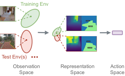
Figure 1: Transforming different domains into a compact representation space reduces the generalization gap between training and test environments.

Recent years have witnessed the increasing popularity of robot learning, yet data scarcity and generalization remain critical challenges. While simulators may serve as “data factories”, learned policies often face performance degradation, because of the sim-to-real gap, i.e., the data distribution shift between the simulated and the real world [12]. For reliable robot performance, robustness against such domain shifts is essential. Our work studies one mechanism that enables learned policies to generalize across domains (Fig. 1).

We target the task of visual navigation. Given a goal location, the robot receives an RGB image as observation at each time step and then predicts a motion command for actuation. Our objective is to learn a policy entirely in simulation, and enable it to generalize to the real world. This is challenging, because the high-dimensional input space, consisting of all possible visual images, induces enormous variability. Our idea is to inject inductive bias into the learning system [8], in particular, a structured representation.

How do we acquire such a representation? It should fulfill two conditions. First, it captures sufficient information for the end task objective, e.g., predicting control commands. Second, to be robust against domain shifts, it contains little extraneous information and has low information entropy. We expect such a representation to be invariant across domains. Clearly, to achieve invariance, there is a trade-off between representation informativeness and compactness.

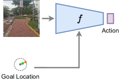
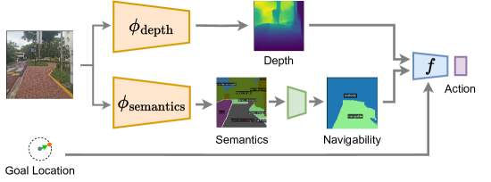
(a)	(b)

Figure 2: A structured representation as an inductive bias for learning robot control policy $f$. (a) The standard end-to-end learning approach (e.g., [1]) uses an image of raw pixels as the input to $f$. (b) Our approach uses pre-trained representation models, $\phi_{\textrm{depth}}$ and $\phi_{\textrm{semantics}}$, to extract invariant representations and improve the generalization performance of the learned policy.

We propose an instance of such representation for visual navigation: SEER, standing for Spatial sEmantic rEpResentation, consists of two features: depth and navigability (Fig. 2). We extract features with pre-trained vision models, learn the mapping from features to control commands in simulation, and test the controller in diverse real-world environments. Our experimental results show that, albeit the simulation is purely indoor environments, our approach enables the policy to generalize effectively to indoor and even outdoor scenes. This significantly outperforms some of the best methods for sim-to-real transfer. We also provide additional experimental evidence that indicates a reduced domain gap in the representation space and thus explains the improved generalizability.

2 Related Work

Generalization is a fundamental question in machine learning and has a vast literature. Within robot learning, for sim-to-real transfer, the two most common approaches are domain randomization (DR) and domain adaptation (DA).

The main idea behind DR is to randomize the training domain so that the test domain appears as one variation of training. DR has been effective in robotic manipulation [11], but has shown limited success in navigation because of the difficulty of achieving sufficient data coverage over the diverse open-world environments in which a mobile robot might operate. On the other hand, DA seeks to learn a mapping from one domain to the other so that the observations in the training and test domains appear similar. However, learning such a mapping requires a large amount of data from both domains and the optimization is often difficult. Both VR-Goggles [7] and BDA [16] use CycleGAN [18] to transform visual observations at test time back to the training domain, but CycleGAN is known to be weak at modeling geometric transformations [18], limiting the applicability of the sim-to-real approach.

In this work, we believe that injecting invariance is a scalable and practical way of achieving generalization [8]. Our approach is related to the work on mid-level representations [2, 5]. The earlier work proposes a maximum coverage feature set comprised of four features (i.e., surface normal, 2D keypoints, 2D segmentation, semantic segmentation) and shows it has significant information overlap with all 26 features in [3] and leads to good generalization performance for control policies. Our work proposes a novel set of only two features, demonstrating that this compact feature set provides much better generalization for visual navigation. Further, we connect the empirical performance to theories on generalization [4] and point out that the gap between different environments is reduced in our representation space, validating our approach and gaining a theoretical understanding for further investigation.

3 Technical Approach

To enable a policy to generalize across domains, the representation could act as an abstraction that filters out task-irrelevant details. The more compact a representation is, the more it is invariant to visual observation $o_{t}$ from different distributions, whereas the less information it could potentially provide to the downstream module $f$.

To formalize this intuition, we use discrete random variables $\mathcal{X}$, $\mathcal{Y}$, and $\mathcal{Z}{}$ to represent observation, representation, and the predicted controls respectively. Since each variable predicts the subsequent one, $\mathcal{X}\rightarrow\mathcal{Y}\rightarrow\mathcal{Z}$ forms a Markov chain, and the model’s predictive uncertainty can be decomposed and bounded by the cardinality of the objective and some information entropy terms:

$$H(\mathcal{Z}|\mathcal{X}) =\operatorname*{\mathbb{E}}\left[\log p(\mathcal{Z}|\mathcal{X})\right]$$

$$=\operatorname*{\mathbb{E}}\left[\log p(\mathcal{Z}|\mathcal{Y})+\log p(\mathcal{Y}|\mathcal{X})\right]$$

$$=H(\mathcal{Z}|\mathcal{Y})+H(\mathcal{Y}|\mathcal{X})$$

$$=H(\mathcal{Z})-I(\mathcal{Z};\mathcal{Y})+H(\mathcal{Y}|\mathcal{X})$$

$$\leq H(\mathcal{Z})-I(\mathcal{Z};Y)+H(\mathcal{Y})$$

$$\leq\log({|\mathcal{Z}|})-I(\mathcal{Z};\mathcal{Y})+H(\mathcal{Y})$$

where $I(\mathcal{Z};\mathcal{Y})$ denotes the mutual information between $\mathcal{Z}$ and $\mathcal{Y}$, and ${|\mathcal{Z}|}$ is the cardinality of $\mathcal{Z}$. The inequality shows that, to make a model make confident predictions, i.e., to minimize $H(\mathcal{Z}|\mathcal{X})$, we can minimize $H(\mathcal{Y})$, the information contained in the representation, and maximize $I(\mathcal{Z};\mathcal{Y})$, the relevance of information in representation with respect to the final objective. Thus, these two terms conceptualize compactness and informativeness respectively. It is worth noting that $H(\mathcal{Y})$ is bounded by $\log({|\mathcal{Y}|})$, thus it is a useful heuristic in practice that we use representations that lie in low-dimensional space.

In this work, we introduce one instance of such representation for navigation. We conjecture that the world can be decomposed into geometry and semantics, both are useful to predict the control commands:

• Geometry: 3D occupancy of points in the space, which encapsulates information about the presence of obstacles, e.g., walls and trees.

• Semantics: Attributes associated with the points in the space, which may capture traversability, e.g., a path is drivable while a wall is an obstacle.

These two pieces of information can be readily extracted with pre-trained depth estimation and semantic segmentation models. Specifically, we find Mask2Former [6] and DPT [13] to work well for in-the-wild data without fine-tuning.

In addition, we observe that the semantic segmentation mask contains redundant information, e.g., the agent does not need to differentiate between a tree and a wall to avoid a collision. Thus, we make the representation more compact by converting object categories to navigability measures (Table 1). It can be observed that this conversion significantly reduces the domain gap (Fig. 5).

Table 1: Mapping of object categories to navigability.

Navigability	Object Category
Obstacle	person, bicycle, car, motorcycle, airplane, bus, train, truck, window-other, tree-merged…
Ambiguous/ Unrelated	ceiling-merged, sky-other-merged, mountain-merged, dirt-merged…
Free space	gravel, playing field, stairs, floor-other-merged, pavement-merged, rug-merged, floor-wood…

4 Experiments

4.1 Setup

We seek to examine the following hypotheses to show that our method is compact, informative, and effective in enabling sim-to-real transfer.

1. Our representation enables the policy to zero-shot transfer from simulated indoor to real outdoor environments, significantly outperforming GAN-based domain adaptation approaches.

2. Reducing semantics categories to navigability is effective in improving the controller’s generalizability to semantically different environments.

3. Our representation is compact. Both geometry and navigability are essential, omitting one of which causes performance degradation.

4. Our representation is informative to the end task. Injecting more information may not improve task performance.

To quantify performance, we repeat each task $N$ times and compute success rate (SR) and success weighted by path length (SPL), defined as

$$SR{}=\frac{1}{N}\sum_{i=1}^{N}s_{i}\quad SPL{}=\frac{1}{N}\sum_{i=1}^{N}s_{i}\frac{l^{*}_{i}}{l_{i}}$$

where $s_{i}$ is a boolean variable indicating success in the i-th trial, $l^{*}_{i}$ is the shortest path length achievable, and $l_{i}$ is the actual path length traversed by the controller. We evaluate all policies in five environments, with increasing levels of domain shifts (Fig. 4). Here are the baselines.

1. RGB. An RGB-based policy learned from scratch.

2. BDA-Real2sim. A policy using CycleGAN to transform real-world observations to the simulator domain, following the most recent work [7, 16].

3. MaxCover. An agent using the max coverage feature set [2] as the representation.

4. SEER w/o Sem2nav. An ablation model that does not convert semantics to navigability. Basically, the control module $f$ directly takes in the segmentation mask and depth prediction as the input.

5. SEER w/o Semantics. An ablation model with only depth as input.

6. SEER w/o Depth. An ablation model with only navigability as input.

For a fair comparison, we train all controllers with the same algorithm and data.

4.2 Implementation

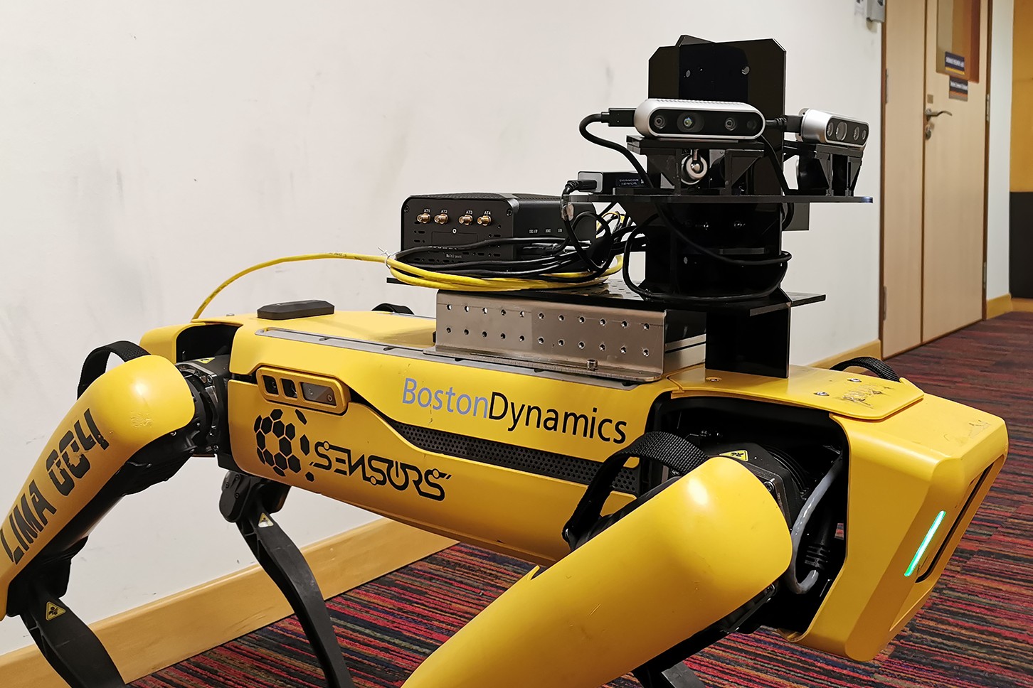
Figure 3: Real-world system setup.

We use a photo-realistic indoor simulator, Habitat [10], for policy learning. We use the training split in [17] that contains 72 maps, and we evaluate the policy in another 5 maps for simulation-based testing.

To generate labeled data for imitation learning, we use a path planner to find the shortest path between randomly sampled initial and goal locations using the ground-truth mesh. The action space is {turn_left, turn_right, go_forward}, as specified by the simulator. We collect 100 trajectories in each training environment. Each sample is a 4-tuple of current pose $s_{t}$, goal pose $s_{goal}$, RGB observation $o_{t}$, and the expert action $a_{t}$.

We parallelly run 36 simulator processes to generate expert demonstrations, which takes 4 hours to finish and we end up having $740K$ samples. Finally, we train the policy model by minimizing the cross-entropy loss between the prediction and the expert actions. We use the AdamW optimizer [9] with an initial learning rate of $1e\text{-}3$ and a batch size of $200$. Training is completed in approximately two days with 2 $\times$ RTX2080Ti.

For real-world testing, we use the Boston Dynamics Spot robot as a physical platform, which is connected to an NVIDIA AGX Xavier onboard computer (Fig. 3). We use the RGB stream of one Intel RealSense D435i RGB-D camera as the agent observation and visual odometry from the Spot robot for localization.

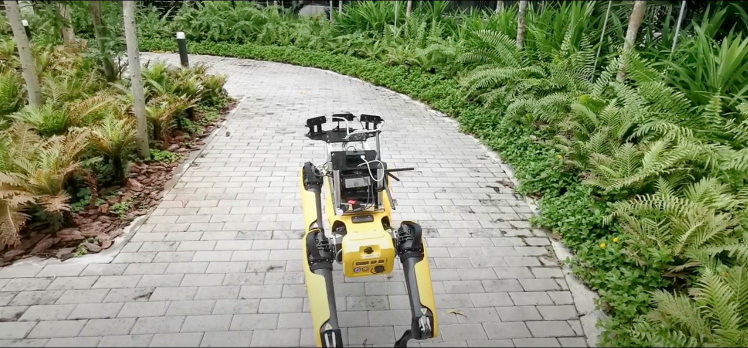
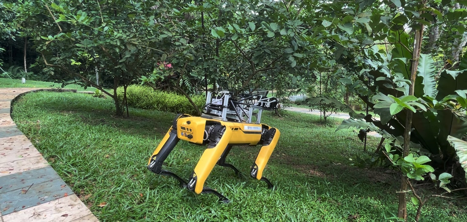
Training	Testing
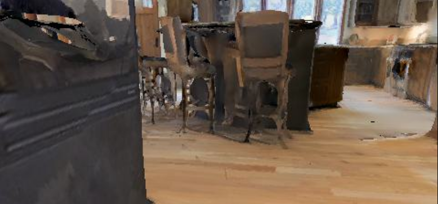
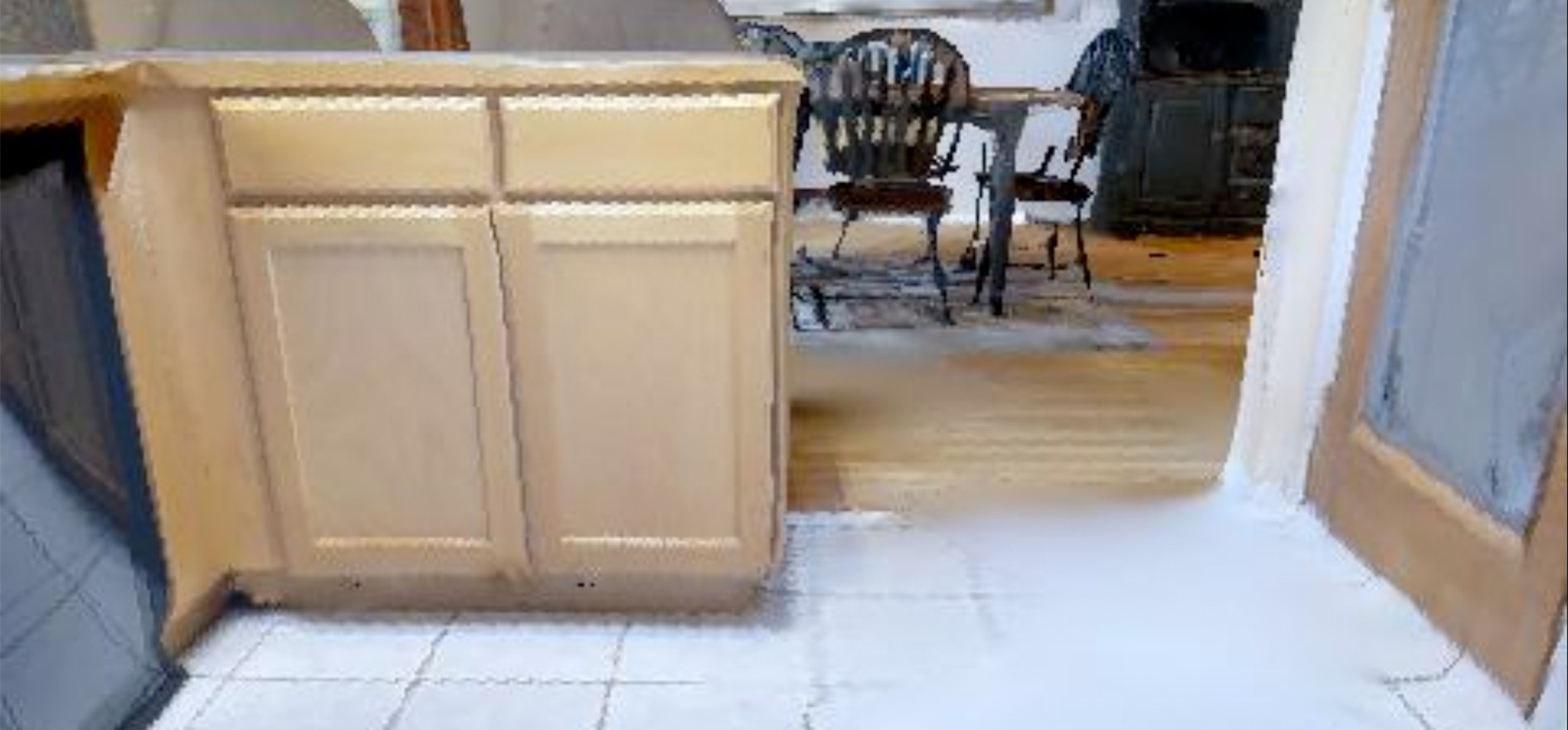
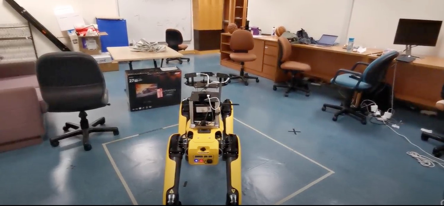
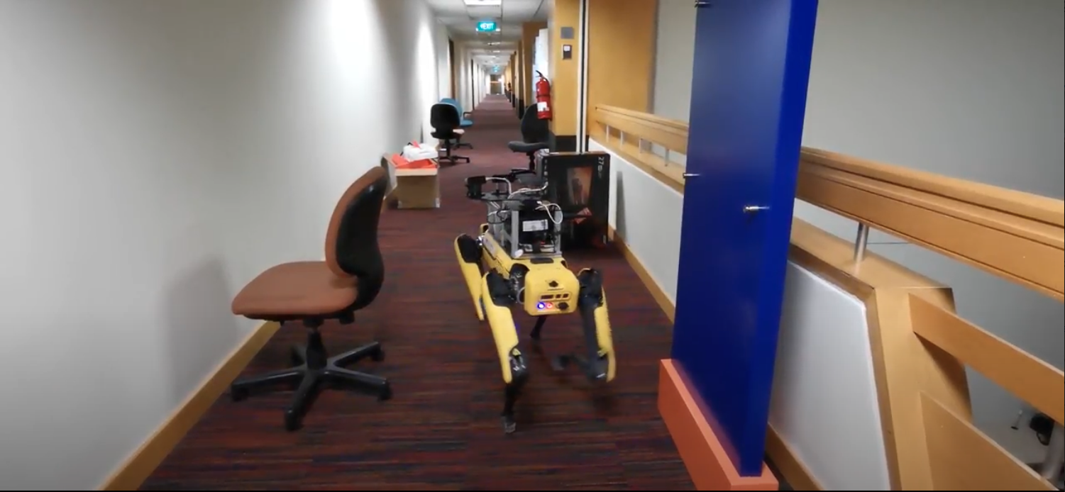
(0) Indoor Simulation	(1) Indoor Lab (2) Indoor Corridor (3) Outdoor Pavement (4) Outdoor Grassland

Figure 4: Third-person view of the training and testing environments. Only data collected in Env0 is used to train the controller. It can be observed that the testing environment differs significantly from the simulation in terms of visual features and spatial geometry.

4.3 Results

Table 2: Navigation experiment results. Best performance in bold.

Model	Env0 Simulation (N = 25)		Env1 Lab (N = 5)		Env2 Corridor (N = 5)		Env3 Pavement (N = 5)		Env4 Grassland (N = 5)		Average
	SR	SPL	SR	SPL	SR	SPL	SR	SPL	SR	SPL	SR	SPL
RGB	0.72	0.68	0	0	0	0	0.40	0.39	0.20	0.17	0.26	0.25
BDA-Real2sim [16]	0.68	0.63	0.60	0.58	0.60	0.59	0.80	0.71	0.60	0.54	0.65	0.61
MaxCover [2]	0.76	0.72	0	0	0.40	0.35	0.60	0.49	0.20	0.11	0.39	0.33
SEER	0.80	0.76	1	0.92	0.80	0.71	1	0.94	0.80	0.64	0.88	0.79
SEER w/o Sem2nav	0.72	0.67	0.40	0.37	0.40	0.32	0.20	0.17	0.40	0.37	0.42	0.38
SEER w/o Depth	0.64	0.62	0.80	0.73	0.60	0.53	1	0.93	0.20	0.12	0.65	0.59
SEER w/o Semantics	0.72	0.68	0.60	0.53	0.60	0.70	0.20	0.16	0.60	0.48	0.54	0.51

	Env0 Simulation	Env1 Lab	Env2 Corridor	Env3 Pavement	Env4 Grassland
RGB
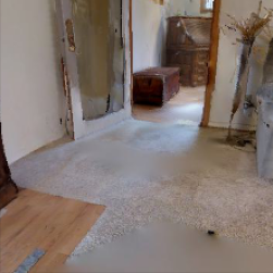
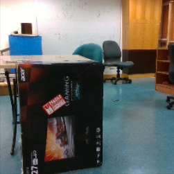
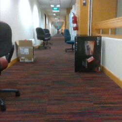
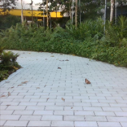
Depth
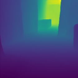
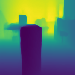
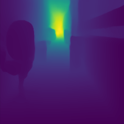
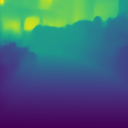
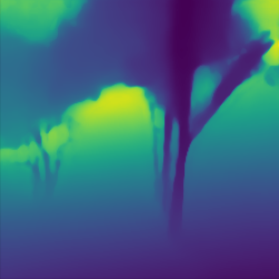
Semantics
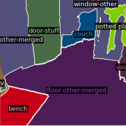
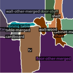
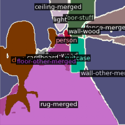
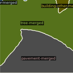
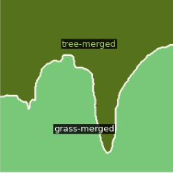
Navigability

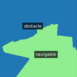
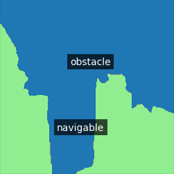
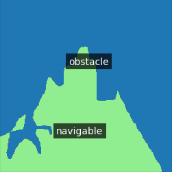
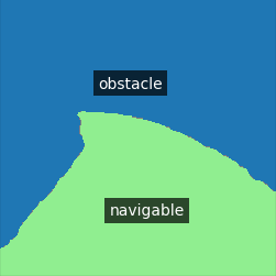
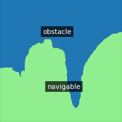
Figure 5: Representations during navigation experiments. It can be observed that the environments appear more visually similar in the depth and navigability space. However, with navigability alone, the agent suffers from size-distance ambiguity in geometrically complex environments, such as the grassland, in which case depth information is particularly helpful for obstacle avoidance.

Full results are summarized in Table 2. Overall, our proposed approach outperforms all baselines across all environments. As expected, RGB is unable to generalize to the real world, due to domain shifts in color, obstacle type, texture, and other variabilities. BDA-Real2sim improves upon RGB by transforming the observation image back to the simulator domain, and the improvement is pronounced in real-world indoor scenes, where RGB fails drastically. In outdoor scenes, it is not comparable with SEER, as it produces distorted and unnatural images when the source differs significantly from the target domain (H₁).

Next, by comparing SEER with SEER w/o Sem2nav across different environments, we observe that the performance gap between controllers increases when the testing environment deviates from the simulation. Specifically, SEER maintains an SR of above 0.8, but that of SEER w/o Sem2nav ranges from 0.2 to 0.4. This shows that converting semantic categories helps the controller generalize to semantically different scenes (H₂).

We can also find out why we need both semantics and depth in our representation. If we compare the performance of SEER w/o Depth, and SEER w/o Semantics in Env3 and Env4, we would find that SEER w/o Depth has a much better performance in Env4 (SR 0.6 vs 0.2), whereas SEER w/o Semantics is significantly better in Env3 (SR 1 vs 0.2). This is because Env3 is an open free space where the geometry is simple and the pavement boundary can be segmented out by semantics. On the other hand, Env4 has homogeneous semantics and obstacles, i.e., trees. Without geometry information, the model suffers from size-distance ambiguity. This loss of information increases the chance of collision. These show that both depth and navigability are important (H₃).

Lastly, MaxCover uses the feature set that has the most information overlap with all visual features, among all possible combinations of the same set size (k = 4) [3]. We can see it has better performance than RGB in Env0, Env2, and Env3, but not in other environments. In contrast, SEER has a consistent and strong performance across all environments, including outdoor scenes. This shows that our representation is informative to the task (H₄).

Above all, we show that our representation is compact and informative, which effectively improves the generalization of the learned policy.

4.4 Further Analysis

Further, we seek to understand how representations improve generalization performance. One way is to estimate the difference between domains in the representation space, and the difference can be estimated by samples, i.e., representations of the agent while operating in different environments. If some representation reduces the difference, it helps preserve the performance across environments.

However, finding such a distance measure is non-trivial. Geometry-based measures, such as L1 and Wasserstein distance, are not invariant to the numerical scale of the data. For example, simply linearly scaling RGB values to $[0,1]$ reduces the distance between two samples, though this linear transformation should not change the domain gap. On the other hand, density-based measures, such as KL-divergence, cannot be estimated accurately with Monte Carlo methods on our high-dimensional data.

Instead, we find $\mathcal{A}$-distance [4] suitable for our purpose. We define a domain as a distribution $\mathcal{D}$ on an instance set $\mathcal{S}$. For sim-to-real transfer, we have a source domain $\mathcal{D}_{S}$ and a target domain $\mathcal{D}_{T}$. The task is to predict a label $\mathcal{Z}$, i.e., control, and we assume $\mathcal{Z}\in[0,1]$. The ground-truth mapping from $\mathcal{D}$ to $\mathcal{Z}$ is defined as $h$. Given a representation function $\phi$ that maps $\mathcal{D}$ to a feature space $\mathcal{Y}$, the features induce distributions $\tilde{\mathcal{D}}_{S}$ and $\tilde{\mathcal{D}}_{T}$, as well as $\tilde{h}$, which is the ground-truth mapping from $\mathcal{Y}$ to $\mathcal{Z}$. Under an imitation learning setup, we learn a predictor $f$ from data, which is an approximation of $h$, then the one-step error rate of $f$ can be defined as the difference between its prediction and the output from the label-generating function $h$. Here we formalize the error rate under distribution $\mathcal{D}_{S}$:

$$\epsilon_{S}(f) =\operatorname*{\mathbb{E}}_{y\sim\tilde{\mathcal{D}}_{S}}\left[\tilde{h}(y)-f(y)\right]$$ (1)

The error under the target distribution, $\epsilon_{T}(f)$, can be defined similarly. Further, as behavior cloning suffers from the compounding error issue [15], the cost of rolling out policy $f$ in the target domain for $T$ steps is $\mathcal{O}(T^{2}\epsilon_{T}(f))$.

Next, we define a learner in the hypothesis space $\mathcal{H}$ which performs optimally on the source and the target domains, i.e.

$$f^{*}=\operatorname*{arg\,min}_{f\in\mathcal{H}}(\epsilon_{S}(h)+\epsilon_{T}(h))$$ (2)

and we denote the total error rate of $f^{*}$ as $\lambda$, i.e., $\lambda=\epsilon_{S}(f^{*})+\epsilon_{T}(f^{*})$. According to [4], we have the following generalization error bound:

Theorem 4.1.

With probability as least $1-\delta$, for every $f$ in hypothesis space $\mathcal{H}$ of Vapnik-Chervonenkis (VC) dimension $d$, the following holds

$$\epsilon_{T}(f) \leq\hat{\epsilon}_{S}(f)+d_{\mathcal{H}}(\tilde{\mathcal{U}}_{S},\tilde{\mathcal{U}}_{T})+\lambda$$

$$\quad\qquad+\frac{4}{m}\sqrt{(d\log\frac{2em}{d}+\log\frac{4}{\delta})}+4\sqrt{\frac{d\log(2m^{\prime})+\log(\frac{4}{\delta})}{m^{\prime}}}$$ (3)

where $\tilde{\mathcal{U}}_{S}$ and $\tilde{\mathcal{U}}_{T}$ are unlabelled samples of size $m^{\prime}$ each drawn from $\tilde{\mathcal{D}}_{S}$ and $\tilde{\mathcal{D}}_{T}$ respectively, $d_{\mathcal{H}}$ is the $\mathcal{A}$-distance, and $e$ is the natural logarithm base.

The intuition behind the theory is that, the error bound under the target distribution can be decomposed into the error under the source distribution, the lowest achievable error, the domain gap, plus some terms dependent on the complexity of the function and the dataset size. For our purpose, what is important is that it explains the relation between the domain gap and model performance, and the $\mathcal{A}$-distance can be estimated from the error rate of an optimal binary classifier on the task of discriminating between samples from the two distributions. Formally, the distance is defined as

$$d_{\mathcal{A}}(\tilde{\mathcal{U}}_{S},\tilde{\mathcal{U}}_{T})=2(1-2\min_{f^{\prime}\in\mathcal{H}}err(f^{\prime}))$$ (4)

where $err$ is the binary classification error, i.e.,

$$err(f^{\prime})=\frac{1}{2m^{\prime}}\sum^{2m^{\prime}}_{i=1}|f^{\prime}(z_{i})-I_{z_{i}\in\tilde{\mathcal{U}}_{S}}|$$ (5)

where $I$ is the indicator function. Note that here $\mathcal{H}{}$ is shared in Eq. (4.1) and Eq. (4). On our task, given that our controller $f$ is a deep neural network, it is infeasible to find $\min_{f^{\prime}\in\mathcal{H}}err(f^{\prime})$ in Eq. (4), which is a global optimum in $\mathcal{H}{}$. To sidestep the difficulty, we use a linear model as an approximation, i.e.

$$d_{\mathcal{A}}(\tilde{\mathcal{U}}_{S},\tilde{\mathcal{U}}_{T}) \approx 2(1-2\min_{f^{\prime}\in\mathcal{H}^{\prime}}err(f^{\prime}))$$ (6)

where $\mathcal{H}^{\prime}$ is the hypothesis space of the linear classifier.

Table 3: $\mathcal{A}$-distance from the testing environment to the training environment in the representation space.

Representation	Env1 Lab	Env2 Corridor	Env3 Pavement	Env4 Grassland
RGB	1.95	1.73	1.99	1.80
BDA-Real2sim	1.93	1.62	1.94	1.74
depth	1.07	1.63	1.39	1.27
semantics	1.24	1.14	1.38	1.95
navigability	1.18	1.11	1.17	1.40
SEER	1.36	1.63	1.65	1.82
2D Segmentation	1.61	1.46	1.88	1.59
2D keypoints	1.85	1.61	1.87	1.67
surface normal	1.83	1.77	1.92	1.90

The estimated $\mathcal{A}$-distance under different representation spaces is presented in Table 3. It can be observed that our selected representations, depth and navigability, minimize the $\mathcal{A}$-distance between the target domain and the source domain among all candidates. It is interesting to see that the domain gap of Env1 and Env4 is minimized in the depth space, which is intuitive: the obstacles in these environments are cluttered and less than 5 meters away, similar to the simulated household scenes during training time. The other two environments are made close to the training environment by the navigability representation, possibly because the navigable regions are narrow with obstacles on the sides, whereas the other environments have a large open space with scattered non-navigable regions. The results are consistent with our intuitive perception of these environments.

Comparing the domain gap in different representation spaces, we find that RGB has the largest $\mathcal{A}$-distance, and BDA-Real2sim reduces the distance by a margin as expected. Comparing semantics and navigability, we can see that our conversion is effective in narrowing the gap, particularly in Env4 where the semantics are completely different from training. This is consistent with our observation from Table 2 that the conversion is very effective in improving the end-task performance.

The estimated $\mathcal{A}$-distance shows that our representation is compact and effectively reduces the domain gap. As pointed out by Theorem 4.1, reducing $\mathcal{A}$-distance lowers the generalization error bound, which explains the performance improvement brought by our representation.

5 Conclusion

This work shows that invariant representations are key to generalization, specifically, in sim-to-real transfer for visual navigation. Our proposed approach enables a local navigation policy trained entirely in simulated indoor environments to generalize to the real world, both indoor and outdoors. We also provide quantitative analyses to show that our representation narrows the domain gap and improves the generalization performance.

Furthermore, we expect the model to be scalable, as it leverages pre-trained models, also known as foundation models [14], to achieve zero-shot transfer to unseen domains. We believe the generalizability of the learned policy improves over time as the foundation models absorb more diverse data during pre-training. On this note, one potentially promising future direction is to explore “foundational representations” for robotics tasks, i.e., representations that emerge from foundation models and capture the minimal sufficient information for decision-making. Having a set of such representations might enable policies to generalize seamlessly to new domains. We hope this work provides insights for future work on the broader key question of generalization in robot learning.

Acknowledgments

This research is supported by Agency of Science, Technology & Research (A*STAR), Singapore under its National Robotics Program (Award M23NBK0053).

References

- [1] Bo Ai, Wei Gao, Vinay, and David Hsu. Deep visual navigation under partial observability. In ICRA, pages 9439–9446. IEEE, 2022.
- [2] Alexander Sax, et al. Learning to navigate using mid-level visual priors. In CoRL, Proceedings of Machine Learning Research, 2019.
- [3] Amir R. Zamir, et al. Taskonomy: Disentangling task transfer learning. In CVPR, pages 3712–3722, 2018.
- [4] Shai Ben-David, John Blitzer, Koby Crammer, and Fernando Pereira. Analysis of representations for domain adaptation. In NeurIPS, pages 137–144, 2006.
- [5] Bryan Chen, et al. Robust policies via mid-level visual representations: An experimental study in manipulation and navigation. In CoRL, volume 155, pages 2328–2346. PMLR, 2020.
- [6] Bowen Cheng, Ishan Misra, Alexander G. Schwing, Alexander Kirillov, and Rohit Girdhar. Masked-attention mask transformer for universal image segmentation. In CVPR, pages 1280–1289. IEEE, 2022.
- [7] Jingwei Zhang, et al. Vr-goggles for robots: Real-to-sim domain adaptation for visual control. IEEE RAL, 4(2):1148–1155, 2019.
- [8] Leslie Pack Kaelbling. The foundation of efficient robot learning. Science, 369(6506):915–916, 2020.
- [9] Ilya Loshchilov and Frank Hutter. Decoupled weight decay regularization. In ICLR. OpenReview.net, 2019.
- [10] Manolis Savva, et al. Habitat: A platform for embodied AI research. In ICCV, pages 9338–9346. IEEE, 2019.
- [11] Marcin Andrychowicz, et al. Learning dexterous in-hand manipulation. Int. J. Robotics Res., 39(1), 2020.
- [12] Nicholas Roy, et al. From machine learning to robotics: Challenges and opportunities for embodied intelligence. CoRR, abs/2110.15245, 2021.
- [13] René Ranftl, Alexey Bochkovskiy, and Vladlen Koltun. Vision transformers for dense prediction. In ICCV, pages 12159–12168. IEEE, 2021.
- [14] Rishi Bommasani, et al. On the opportunities and risks of foundation models. CoRR, abs/2108.07258, 2021.
- [15] Stéphane Ross, Geoffrey J. Gordon, and Drew Bagnell. A reduction of imitation learning and structured prediction to no-regret online learning. In AISTATS, volume 15 of JMLR Proceedings, pages 627–635, 2011.
- [16] Joanne Truong, Sonia Chernova, and Dhruv Batra. Bi-directional domain adaptation for sim2real transfer of embodied navigation agents. IEEE Robotics Autom. Lett., 6(2):2634–2641, 2021.
- [17] Fei Xia, Amir Roshan Zamir, Zhi-Yang He, Alexander Sax, Jitendra Malik, and Silvio Savarese. Gibson env: Real-world perception for embodied agents. In CVPR, pages 9068–9079, 2018.
- [18] Jun-Yan Zhu, Taesung Park, Phillip Isola, and Alexei A. Efros. Unpaired image-to-image translation using cycle-consistent adversarial networks. In ICCV, pages 2242–2251, 2017.