Bayesian Regression Markets

Abstract

Abstract

Machine learning tasks are vulnerable to the quality of data used as input. Yet, it is often challenging for firms to obtain adequate datasets, with them being naturally distributed amongst owners, that in practice, may be competitors in a downstream market and reluctant to share information. Focusing on supervised learning for regression tasks, we develop a regression market to provide a monetary incentive for data sharing. Our proposed mechanism adopts a Bayesian framework, allowing us to consider a more general class of regression tasks. We present a thorough exploration of the market properties, and show that similar proposals in current literature expose the market agents to sizeable financial risks, which can be mitigated in our probabilistic setting.

1 Introduction

Data is the lifeblood of machine learning, yet for many firms, obtaining datasets of sufficient quality remains a challenge, with them being naturally distributed amongst owners with heterogeneous characteristics (e.g., privacy preferences). This has motivated several developments in the field of collaborative analytics, also known as federated learning (Figure 1(a)), where models are trained on local servers without the need for data centralization, thereby preserving privacy and distributing the computational burden (Kairouz et al., 2019). However, this framework provides only an incentive-free means for data sharing, relying on the critical assumption that owners are willing to collaborate (i.e., by sharing their private information) altruistically. This rather strong assumption may be violated if owners are competitors in a downstream market environment (Gal-Or, 1985). Consequently, a fruitful area of research has emerged that proposes to instead commoditize data within a market-based framework, where compensation (e.g., remuneration) can be used as an incentive for collaboration (Bergemann and Bonatti, 2019).

(a) Collaborative Analytics

(b) Data Markets

(c) Analytics Markets

Figure 1: Schematic illustration of existing frameworks for data sharing with multiple buyers and sellers, where each figure depicts a building block consisting of a single interaction. The blue, red and green arrows indicate computational, information and monetary transactions between the buyer and the seller, respectively.

Information economics has been a prominent concept in game theory literature since the 1980s (Gal-Or, 1985), with early works focused on incentive-free data sharing, both publicly (Morris and Shin, 2002) and within local information channels (Dahleh et al., 2016). Over the last decade, data monetization has been an increasingly discussed topic, for which the first proposals considered data markets (Figure 1(b)), allowing buyers to purchase raw data from sellers through bilateral transactions (Rasouli and Jordan, 2021). Whilst this offers a seemingly practical way to acquire data from others, the value of the data to the buyer typically depends on the analytics task at hand, hence pricing raw data in these markets is difficult (Cong et al., 2022), especially in the context of privacy-preservation (Acemoglu et al., 2022). Instead, one can acknowledge that the reason a firm may procure data in the first place is often to enhance capabilities in some analytics task. Rather than viewing the value of data as an intrinsic property, it can instead be a function of any enhancement in said capabilities it can provide (Agarwal et al., 2019). This leads to opportunities for combining the notion of data markets with collaborative analytics to form analytics markets (Figure 1(c)), whereby the buyer owns an analytics task (e.g., a machine learning model) and seeks to enhance its capabilities (e.g., predictive performance) by harnessing the data, and possibly the compute, of the sellers. The buyer pays for the overall capability enhancement, for which each seller is compensated based on its marginal contribution. As in Pinson et al. (2022a), we are interested in applications in which the analytics task describes a regression model along with the process for inference used for training (i.e., our attention centers on regression markets). This builds on current literature concerning data elicitation from strategic (Dekel et al., 2010) and privacy-sensitive (Cummings et al., 2015) owners. In this context, owners of regression models seek to enhance predictive performance, for which they have a private valuation (e.g., their value of forecast accuracy in a downstream decision-making process). Their public bids, which may not equal private valuations, are then used to set the price. Sellers propose their own data as features and are remunerated based on their marginal contributions to the improved model-fitting. The market revenue is therefore a function of both the market price and the overall enhancement in predictive performance. In related work, these regression tasks are often introduced from a frequentist perspective, which seems to contradict current trends towards probabilistic forecasting across many industries (Gneiting and Katzfuss, 2014). This would instead favour probablistic regression models capable of directly providing the distribution of the target signal, rather than merely point-estimating a particular characteristic thereof (e.g., the expected value). Even though frequentist methods can indeed be used for probabilistic forecasting (e.g., by interpolating point-estimated quantiles), disregarding uncertainty in parameter estimation can yield overly confident predictions that miss-represent the true level of variability in the data. Accordingly, there is an incentive to adopt Bayesian inference, a principled framework for modelling parameter uncertainty that, in fact, subsumes many frequentist regression methods, thereby providing richer and more nuanced information about future outcomes. Our contribution is the development of a regression market that enables Bayesian methods for regression, allowing us to consider a more general class of probabilistic regression tasks. We provide a thorough exploration of the market properties with a focus on fair allocation of market revenue. We further show that frequentist-based mechanism designs in the current literature expose the market agents to considerable financial risks, which we mitigate by re-formulating the value of a feature in terms of the information gain it provides. The remainder of the paper reads as follows: Section 2 introduces the market agents and the design of our proposed market mechanism. Section 3 assesses the theoretical market properties of our proposal and presents methods for mitigating financial risks exhibited by the agents. Section 4 and Section 5 illustrate our findings through a set of simulation-based and real-world case studies, respectively. Finally, Section 6 gathers our conclusions and perspectives for future work.

2 Preliminaries

Our proposed mechanism is intended to be hosted on a platform capable of handling both the analytical (e.g., parameter inference) and market-based (e.g., revenue allocation) components together in tandem. As the market will comprise multiple agents, we define a transaction as an exchange between a single central agent (i.e., a buyer) and multiple support agents (i.e., sellers), at a particular point in time, whereby the central agent seeks to enhance the predictive performance of a regression task, for which the support agents propose their own data as input features. Whilst this definition preserves the capacity for parallel transactions, we assume each is independent, thereby disregarding data exclusivity, wherein the same data can only be sold a finite number of times (Cao et al., 2017), as well as any externalities this may exert (Agarwal et al., 2020). Although there may be multiple sellers, the enhancement in performance received by the central agent is perceived to be a function of the complete set of information available. We hence view a transaction as being between the central agent and a single monopolistic support agent, a single agent with access to the complete set of features and only one item for sale, specifically the available loss reduction. The private valuation is assumed to equal the public bid (i.e., the valuation for a marginal improvement in model fitting). The central agent is then allocated the full performance enhancement offered by the monopolistic support agent, and the payment collected is a function of these two values. One can view this as a specification of the mechanism proposed in Agarwal et al. (2019), where the monopolistic support agent offers several possible performance enhancements, each representing varying degrees of obfuscation of the true data, characterized by the discrepancy between the bid of the central agent and the market price. Since we assume the market price to be exogenous, our work is concerned specifically with the regression analysis and subsequent revenue allocation, as opposed to the pricing mechanism.

2.1 Market Agents

Let $\mathcal{A}$ denote the set of market agents, one of which $c\in\mathcal{A}$ is the central agent seeking to enhance their forecasts. The remaining agents $a\in\mathcal{A}_{-c}$ are support agents that propose data as input features, whereby $\mathcal{A}_{-c}=\mathcal{A}\setminus\{c\}$. The central agent is characterized by an interest in a particular stochastic process $\{Y_{t}\}$, defined as a set of successive random variables $Y_{t}$ indexed over discretized time steps $t$. Eventually, a time-series $\{y_{t}\}$ is observed, comprising realizations from $\{Y_{t}\}$ (i.e., one per time step). Instead of assuming that a particular characteristic of $Y_{t}$ is sought (e.g., the expected value, a specific quantile, etc.), we rather model the entire distribution, albeit conditioned on the observed data; the characteristic extracted by the central agent is simply treated as some downstream decision-making process. We write $\textbf{x}_{\mathcal{I},t}$ as the vector of input features at time $t$, indexed by the ordered set $\mathcal{I}$. Each agent $a\in\mathcal{A}$ owns a subset $\mathcal{I}_{a}\subseteq\mathcal{I}$ of indices, such that the features are distributed amongst the market agents as follows: the central agent $c$ owns the subset $\mathcal{I}_{c}\subset\mathcal{I}$. Each support agent $a\in\mathcal{A}_{-c}$ also owns a subset, with indices $\mathcal{I}_{a}\subset\mathcal{I}$, such that $|\mathcal{I}_{c}|+\sum_{a\in\mathcal{A}_{-c}}|\mathcal{I}_{a}|=|\mathcal{I}|$. We write $\mathcal{I}_{-c}$ as the set of indices for features owned only by the support agents. Since the data is observed at successive time steps, we let $\textbf{x}_{t}=[x_{1,t},\dots,x_{|\mathcal{I}|,t}]^{\top}$ be the vector of values for all features at time $t$. When only a particular subset of features $\mathcal{C}\subseteq\mathcal{I}$ is used, we add an index for the set itself, such that the vector of values for features in $\mathcal{C}$ at time $t$ is denoted by $\textbf{x}_{\mathcal{C},t}$. We write $\mathcal{D}_{\mathcal{C},t}=\{\textbf{x}_{\mathcal{C},t^{\prime}},y_{t^{\prime}}\}_{\forall t^{\prime}\leq t}$ to be the set of input-output pairs for a particular subset of features observed over a set of discrete time indices $t^{\prime}\in\{1,\dots,t\}$ up until time $t$.

2.2 Regression Task

To instigate a transaction, the central agent first posts a regression task to the market platform, which describes the particular model for which they seek to enhance predictive performance. We consider the problem of interpolating through data (i.e., the observations $\{y_{t}\}$) under the assumption that the target signal is subject to noise, whilst the input features are noise-free. Let us define an interpolant as a mapping $f$ between a subset of features $\textbf{x}_{\mathcal{C},t}$ and a real-valued scalar, which may, for instance, represent the expected value of the target signal conditioned on the inputs such that

$$f:\textbf{x}_{\mathcal{C},t}\in\mathbb{R}^{|\mathcal{C}|}\mapsto\mathbb{E}[Y_{t}\,|\,\textbf{x}_{\mathcal{C},t}]\in\mathbb{R},\quad\forall t,\ \forall\mathcal{C}.$$ (1)

We focus solely on parametric regression, and further limit ourselves to functions that can be expressed as linear in their coefficients, with a view to preserve convexity and later guarantee certain market properties. The simplest regression models within this class are those which are also linear functions of the input features, and hence exhibit limited flexibility. We can however obtain a richer class of models by considering linear combinations of a fixed set of nonlinear functions (i.e., basis functions). These models maintain linearity with respect to the parameters, whilst facilitating nonlinearity with respect to the input features. Let $\textbf{w}_{\mathcal{C}}\in\mathbb{R}^{|\mathcal{C}|}$ be a vector of coefficients that is used to parameterize the mapping in (1), which, for notational brevity, we assume to be part of a general set of free parameters $\Theta_{\mathcal{C}}$ that shall be inferred from data. We write $\psi(\textbf{x}_{\mathcal{C},t})$ to be the vector of basis functions specified by the central agent, such that the linear interpolant is given by

$$f(\textbf{x}_{\mathcal{C},t},\textbf{w}_{\mathcal{C}})=\textbf{w}_{\mathcal{C}}^{\top}\,\psi(\textbf{x}_{\mathcal{C},t}),\quad\forall t,\ \forall\mathcal{C},$$ (2)

where we assume that the vector of basis functions under consideration invariably incorporates a dummy basis function (i.e., $\psi_{0}(\mathbf{x}_{\mathcal{C},t})=1,\,\forall t$) which is included as part of the feature set owned by the central agent. We note that in general the central agent need not own any feature themselves, in which case only this dummy term is provided and all predictive performance is supplied by the features owned by support agents. From a probabilistic perspective, it is favourable to describe the entire target distribution, rather than simply a particular characteristic thereof, in effort to express the uncertainty in the target signal for each value of the input features. We model the target variable as a deviation from the deterministic mapping in (2) under a zero-mean additive noise process, the parameters of which are also held in $\Theta_{\mathcal{C}}$. In frequentist regression analyses, the free parameters in $\Theta_{\mathcal{C}}$ would be treated as unknown yet fixed quantities, with the observed data perceived as random samples from an underlying stochastic process. Hence, any uncertainties in the parameter estimates (e.g., sampling variability, measurement error, misspecification, etc.) are disregarded. In contrast, Bayesian inference treats the parameters themselves as random variables and aims to infer their distribution by incorporating prior beliefs, which are updated as new data is observed. Let $\mathcal{H}$ denote a hypothesis, a set of fixed assumptions that restricts the space of possible regression models. The hypothesis contains the vector of basis functions, as well as the functional forms of two probability distributions, namely a prior distribution (i.e., plausible parameter values) and a likelihood (i.e., the probability of the data conditioned on the parameters). The regression task posted to the market platform by the central agent at time $t$ is therefore fully described by a hypothesis and the observed data.

2.3 Market Clearing

Each of the support agent posts their feature(s) to the platform in hope to receive monetary compensation, albeit without knowing the value of their data a priori. We suppose each support agent is willing to accept any nonnegative payment if their data is deemed useful. However, we acknowledge that in practice, support agents may indeed prefer to condition their participation on a minimum payment to, for instance, reflect privacy costs (Acquisti et al., 2016; Han et al., 2022b). Whilst the intention is to fairly allocate revenue amongst features based on marginal contributions to the overall improvement in some objective, in reality, certain features may worsen predictive performance and have a negative impact to the central agent, hence we make the following assumption.

Assumption 1

Given the specified hypothesis, a feature selection process (e.g., cross-validation or marginal likelihood optimization) is performed by the market operator a priori (i.e., before market clearing), such that only features capable of imposing a nonnegative impact on the objective are considered.

For discussions on conventional feature selection problems, cross-validation in a Bayesian context and methods for marginal likelihood optimization, the reader is referred to Guyon and Elisseeff (2003), Watanabe and Opper (2010) and Fong and Holmes (2020), respectively. Once the entire set of required market inputs have been received, the market operator is tasked with clearing the market. In addition to feature selection, this procedure involves several steps, namely parameter inference, performance evaluation, payment collection and revenue allocation.

2.3.1 Parameter Inference

Based on all of the observations up until time $t$, we can summarize our updated beliefs about the parameters through the posterior distribution, which, by virtue of Bayes theorem, is proportional to the product of the likelihood and the prior such that

$$p(\Theta_{\mathcal{C}}|\mathcal{D}_{\mathcal{C},t})\propto p(\mathcal{D}_{\mathcal{C},t}|\Theta_{\mathcal{C}})p(\Theta_{\mathcal{C}}),\quad\forall t,\ \forall\mathcal{C}.$$ (3)

For an arbitrary choice of prior, the posterior may not be available in closed-form, requiring methods for approximate Bayesian inference (e.g., Monte-Carlo integration) to be employed. However, for a known functional form of the likelihood, priors that are conjugate can result in posteriors with tractable, well-known densities. Although we can indeed use the entire set of observations to evaluate the posterior (i.e., batch inference), it may be more appropriate to allow the moments of this distribution to vary in time, thereby accounting for nonstationarities in any of the underlying processes that can lead to concept drift. In a Bayesian treatment of linear regression, batch inference can be viewed as a specification of a more general online learning problem, whereby the parameters are updated in a recursive manner. To see this, we re-write the expression in (3) as a series of sequential updates such that

$$p(\Theta_{\mathcal{C}}|\mathcal{D}_{\mathcal{C},t}) \propto p(\mathcal{D}_{\mathcal{C},t}|\Theta_{\mathcal{C}})p(\Theta_{\mathcal{C}}|\mathcal{D}_{\mathcal{C},t-1}),\quad \forall t,\ \forall\mathcal{C},$$ (4a)

$$=p(\mathcal{D}_{\mathcal{C},t}|\Theta_{\mathcal{C}})\left[p(\Theta_{\mathcal{C}})\prod_{t^{\prime}<t}p(\mathcal{D}_{\mathcal{C},t^{\prime}}|\Theta_{\mathcal{C}})\right],\quad \forall t,\ \forall\mathcal{C}.$$ (4b)

To place greater weight on more recent data, we can augment this update step to use exponential forgetting, where the importance given to past information decreases exponentially. This generally translates to the idea of likelihood flattening, whereby we reformulate (4b) as a trade-off between the posterior at the previous time step and the original prior (i.e., before any data had been observed), thereby emulating a loss in belief with respect to the historic estimates (Peterka, 1981). This trade-off between the two distributions can be framed as the problem of finding the probability density function with minimum expected Kullback–Leibler (KL) divergence (i.e., relative entropy) between them (Kulhavỳ and Zarrop, 1993), which has a unique solution enabling us to replace the prior at time $t$ in (4a) with the following:

$$p(\Theta_{\mathcal{C}}|\mathcal{D}_{\mathcal{C},t-1},\tau) =\mathop{\mathrm{argmin}}_{p^{\ast}}\ \tau\,D_{\textrm{KL}}\left(p^{\ast}\,||\,p(\Theta_{\mathcal{C}}\,|\mathcal{D}_{\mathcal{C},t-1})\right)+(1-\tau)\,D_{\textrm{KL}}\left(p^{\ast}\,||\,p(\Theta_{\mathcal{C}})\right),\quad \forall t,$$ (5a)

$$\propto p(\Theta_{\mathcal{C}}|\mathcal{D}_{\mathcal{C},t-1})^{\tau}p(\Theta_{\mathcal{C}})^{1-\tau},\quad \forall t,$$ (5b)

where the variable $p^{\ast}$ denotes the resultant density function, $D_{\textrm{KL}}(\,\cdot\,||\,\cdot\,)\in\mathbb{R}_{+}$ is the KL divergence and the parameter $\tau\in[0,1]$ is analogous to the forgetting factor in time-weighted Least-Squares fitting (Vahidi et al., 2005). Observe that, as $\tau\mapsto 1$, the prior information available at time $t$ becomes identical to the posterior information at the previous time step as in (4b), emulating batch learning, whereas when $\tau=0$, all of the previous information is forgotten and we resort to the original (i.e., flat) prior. For convenience, we treat $\tau$ as a time-invariant hyperparameter, however for a full Bayesian treatment one could also infer its value jointly, together with $\Theta_{\mathcal{C}}$.

2.3.2 Performance Evaluation

Given a set of observations up until time $t$, we can evaluate the performance of a specific model (i.e., subset of features) by making a prediction for a time step $t^{\ast}$, conditioned on the observed input features. For now, we consider the general case where $t^{\ast}$ is an arbitrary time step to account for both in-sample (i.e., $t^{\ast}\leq t$) and out-of-sample (i.e., $t^{\ast}>t$) situations. In Bayesian regression analyses, a prediction is typically defined to be the computation of the posterior predictive distribution, derived by integrating out the parameters using the convolution of the likelihood with the posterior, given by

$$p(y_{t^{\ast}}|\textbf{x}_{\mathcal{C},t^{\ast}},\mathcal{D}_{\mathcal{C},t})=\int p(y_{t^{\ast}}|\textbf{x}_{\mathcal{C},t^{\ast}},\mathcal{D}_{\mathcal{C},t},\Theta_{\mathcal{C}})p(\Theta_{\mathcal{C}}|\mathcal{D}_{\mathcal{C},t})d\Theta_{\mathcal{C}},\quad\forall\mathcal{C},$$ (6)

which for brevity we hereafter omit the training dataset and write as $p(y_{t^{\ast}}|\textbf{x}_{\mathcal{C},t^{\ast}})$. In order to evaluate predictive performance, we define an objective function $\ell$. If a model describing a particular characteristic of $Y_{t}$ is sought, then this objective function could be set as a direct function of the residuals (i.e., by extracting the corresponding point from the predictive distribution). However, as we intend to provide the entire predictive distribution, we can generally define $\ell$ as a function of the predictive likelihood (i.e., $\ell_{\mathcal{C},t^{\ast}}:p(y_{t^{\ast}}|\textbf{x}_{\mathcal{C},t^{\ast}})\mapsto\mathbb{R}$), assuming the following.

Assumption 2

The mapping $\ell$ is a negatively-oriented strictly proper scoring rule. Accordingly, it holds that: (i) for any two models, the one that provides the more accurate description of the data will render a lower score; and (ii) the lowest score is uniquely obtained when the prediction converges to the true distribution.

In the context of online exponential forgetting, evaluating $\ell$ at each time step can be perceived as a recursive and adaptive time-varying estimator of its expected value; adaptive in the sense that a greater weight is placed on more recent data. Hence, the in-sample estimate of $\mathbb{E}[\ell]$ for a particular subset of features at time $t$ with respect to (6) can be described by the following recursion:

$$\mathbb{E}[\ell_{\mathcal{C}}]_{t}=(1-\tau)\,\ell_{\mathcal{C},t}+\tau\,\mathbb{E}[\ell_{\mathcal{C}}]_{t-1},\quad \forall t,\ \forall\mathcal{C}.$$ (7)

To consider the case of out-of-sample evaluation (e.g., if $t$ is the next available time step) we simply replace $\mathcal{D}_{\mathcal{C},t}$ in (7) with $\mathcal{D}_{\mathcal{C},t-1}$ (i.e., the most recent observations). It should be noted that for Bayesian model comparison, one would generally prefer to consider the marginal likelihood instead, which quantifies the joint probability of the data, thereby penalizing implausible over-parameterized models that may generalize poorly (MacKay, 1992). However, we consider the predictive likelihood sufficient for evaluation given we are solely concerned with predictive performance.

2.3.3 Payment Collection

Once the predictive performance of the complete set of input features has been evaluated, the payment can be collected from the central agent. As well as a regression task, our market requires the central agent to post to the platform their public bid, denoted by $\lambda\in\mathbb{R}_{+}$, which represents an exogenous linear mapping between a unit improvement in $\ell$ and the corresponding downstream monetary reward that would be earned. The market price is solely dependent on this valuation, which instills the ideology that the value of data is derived from the enhanced predictive performance it provides, rather than the raw data itself. We do acknowledge the weakness of this linearity assumption, as in practice, $\lambda$ may be, for instance, a logarithmic function of the central agent’s revenue (i.e., further reductions in $\ell$ may provide diminishing returns), albeit with exponential costs for the support agents. Nevertheless, we leave it as future work to explore the optimal functional form of $\lambda$. Lastly, the total market revenue at time $t$ is equal to the payment collected from the central agent, denoted $\pi_{c,t}$, which is a function of $\lambda$, as well as the overall improvement in the objective, such that

$$\pi_{c,t}=\lambda\,\left(\,\mathbb{E}[\ell_{\mathcal{I}_{c}}]_{t}-\mathbb{E}[\ell_{\mathcal{I}}]_{t}\right),\quad\forall t.$$ (8)

2.3.4 Revenue Allocation

Once the market has been cleared, the natural question that follows is: how can we fairly allocate market revenue amongst support agents? To answer this question, several auction-based setups have been proposed, for both welfare-maximizing and revenue-maximizing mechanisms, pertaining to topics such as privacy preservation (Koutsopoulos et al., 2015), data exclusivity (Cao et al., 2017) and the negative externalities exhibited by the market agents (Agarwal et al., 2020). Other methods bear upon interoperability in machine learning, adopting widely adopted solution concepts (namely, semivalues) for the problem of attribution in cooperative game theory to allocate revenue amongst support agents directly (Dubey et al., 1981). The benefit of this approach being that these solution concepts are generally characterized by a collection of axioms that yield desirable market properties by design (Ghorbani and Zou, 2019), specifically: symmetry, efficiency, null-player and additivity. For a definition of these axioms, the reader is referred to Chalkiadakis et al. (2011). If we frame features as players and their interactions as a cooperative game, the semivalue of a feature can be defined as its expected marginal contribution towards a set of other features, weighted solely based on the size of the sets. For many applications, the semivalue of choice is the Shapley value (Shapley, 1997), the unique value that satisfies all of the four axioms stated previously. Given the set $\mathcal{I}_{-c}$ of indices corresponding to features owned by the support agents, let $v:\mathcal{C}\in\mathcal{P}({\mathcal{I}_{-c}})\mapsto\mathbb{R}$ be a characteristic function that maps the power set $\mathcal{P}(\mathcal{I}_{-c})$ of all features with indices in $\mathcal{I}_{-c}$ to a real-valued scalar, where the set $\mathcal{C}$ denotes a coalition in the cooperative game. If we further let $\mathcal{C}^{\prime}=\mathcal{C}\cup\mathcal{I}_{c}$ for all $\mathcal{C}\subseteq\mathcal{I}_{-c}$, be the union of the set of indices owned by the central agent and a particular subset of indices owned by the support agents, the Shapley value is given by

$$\phi_{i,t}=\sum_{\mathcal{C}\in\mathcal{P}(\mathcal{I}_{-c}\setminus\{i\})}\frac{|\mathcal{C}|!(|\mathcal{I}_{-c}|-|\mathcal{C}|-1)!}{|\mathcal{I}_{-c}|!}\,m_{t}(\{i\},\mathcal{C}^{\prime}),\quad\forall i\in\mathcal{I}_{-c},\,\forall t,$$ (9)

where $m_{t}(\{i\},\mathcal{C})$ describes the marginal contribution of the $i$-th feature to coalition $\mathcal{C}$, conventionally defined as $m_{t}(\{i\},\mathcal{C})=v_{t}(\mathcal{C})-v_{t}(\mathcal{C}\cup\{i\})$ with respect to the characteristic function. The weight in this discrete expectation assigned to each coalition is defined as such to avoid unnecessary calculations of the marginal contribution of the $i$-th feature to permutations of the same coalition, which would have equal value by virtue of the symmetry axiom. For instance, $m_{t}(\{i\},\{j\})\equiv m_{t}(\{i\},\{j\}),\,\forall(i,j)\in\mathcal{I}_{-c},\ i\neq j$, thus it is computationally favourable to avoid making this calculation twice. We acknowledge that there is indeed a rich collection of semivalues to choose from, for example the Banzhaf value (Lehrer, 1988), which is an unweighted average of the marginal contribution of a feature towards coalitions of other features, satisfying all but the additivity axiom, as well as the Leave-one-out value, a simple Vickrey-Clarke-Groves mechanism which attributes each feature its marginal contribution towards the grand coalition. The particular choice of semivalue thus depends on the desired properties of the market. For instance, whilst the Banzhaf value violates the efficiency axiom, it may offer greater robustness to malicious behaviour, whereby a support agent replicates its data, acting under multiple identities to maximize revenue (Han et al., 2022a). Likewise, although simple to implement, the Leave-one-out value may fall short when features are not independent and when the regression model is non-separable or nonlinear. We choose to adopt the Shapley value due to its appealing uniqueness in satisfying the four axioms, the first two of which are often used as a criteria for fairness (van den Brink, 2002). The use of semivalues is this context is, however, not straightforward in general, as there exists several methods for representing a machine learning model as a cooperative game (Covert et al., 2021), each with causal nuances that may be suited to particular contexts (Chen et al., 2020; Janzing et al., 2020). To avoid taking causality into consideration, we hereby make the following simplifying assumption.

Assumption 3

Any two features available in the market are statistically independent (e.g., potentially as a result of Assumption 1), that is, $p(x_{i,t}|x_{j,t})=p(x_{i,t})\ \forall(i,j)\in\mathcal{I},\ i\neq j,\,\forall t$.

We do acknowledge that this is a particularly strong assumption, and encourage an exploration of the causal effects amongst correlated features within our Bayesian framework, and the implications to the market design therein, as future work. This Shapley-based attribution policy can then be used to allocate the market revenue amongst the support agents. First, we need to address that given our estimator of the expected objective varies with time (i.e., in an online learning environment), the attributions are time-varying too, as well as the payment of the central agent described in (8). In line with (7), the estimated expected Shapley value at time $t$ is given by

$$\mathbb{E}[\phi_{i}]_{t}=(1-\tau)\phi_{i,t}+\tau\mathbb{E}[\phi_{i}]_{t-1},\quad\forall i\in\mathcal{I}_{-c},\,\forall t.$$ (10)

Given we evaluate (10) for each feature, the overall payment received by each support agent is simply given by

$$\pi_{a,t}=\sum_{i\in\mathcal{I}_{a}}\lambda\,\mathbb{E}[\phi_{i}]_{t},\quad\forall a\in\mathcal{A}_{-c},\ \forall t.$$ (11)

2.4 Market Stages

Finally, we need to consider the fact that in practice, machine learning pipelines are typically divided into in-sample (i.e., training) and out-of-sample (i.e., testing) stages. The first stage involves parameter estimation using observed input-output pairs, which we accomplish using Bayesian inference to derive the posterior distribution. At the second stage, a trained model is used for genuine forecasting on previously unseen data, testing its capacity to generalize beyond the training set. Given these two stages are distinct, it is necessary to differentiate between in-sample and out-of-sample data valuation. Not only is the isn-sample value of a feature merely an estimate of its actual value towards genuine forecasting, but the central agent’s valuation for an in-sample improvement in the objective will be correlated with the out-of-sample performance of the model, as any downstream decision-making processes typically occur at this stage. We therefore adopt the two-stage regression market model proposed in Pinson et al. (2022a), that is, the value of a feature is assessed based on marginal contributions to both the in-sample and out-of-sample estimates of $\mathbb{E}[\ell]$, albeit in separate transactions.

3 Market Properties

Since we have assumed the market price to equal the public bid of the central agent, the remaining design decision that will influence the properties of the market is related to the Shapley value-based attribution policy, specifically the choice of characteristic function used to value a particular coalition of features. Whilst Shapley values are emerging as the de facto tool for interpreting predictions from complex machine learning models (Guyon and Elisseeff, 2010; Sundararajan and Najmi, 2020; Tsai et al., 2023), their application within a probabilistic context is not yet as well understood. Difficulties arise from the need to compare predictions obtained from different subsets of input features, which can be less straightforward when the model output is a probability distribution as opposed to a scalar. In general, at a given time $t$ we set the characteristic function to be equal to the current estimate of the expected value of the objective as in (7), such that we write the characteristic function as $v_{t}(\mathcal{C})=\mathbb{E}[\ell_{\mathcal{C}}]_{t}$, hence the design decision is not the characteristic function itself per se, but the particular functional form of $\ell$, which recall maps the predictive likelihood to a real value. In this section we introduce the following market designs: (i) $\mathcal{M}^{\mathrm{MLE}}_{\mathrm{NLL}}$ — a frequentist framework based on maximum likelihood estimation (MLE) which values features using the negative logarithm of the posterior predictive likelihood (NLL), (ii) $\mathcal{M}^{\mathrm{BLR}}_{\mathrm{NLL}}$ — the analogue of $\mathcal{M}^{\mathrm{MLE}}_{\mathrm{NLL}}$ now in a Bayesian linear regression (BLR) framework, and (iii) $\mathcal{M}^{\mathrm{BLR}}_{\mathrm{KL}-v}$ and $\mathcal{M}^{\mathrm{BLR}}_{\mathrm{KL}-m}$ — BLR frameworks that instead value features based on the information gain they provide, measured using the KL divergence.

3.1 Likelihood-based Allocation

In related work, such as Agarwal et al. (2019), emphasis is placed on frequentist regression analyses, whereby a point-estimate of the model parameters is obtained. As for our case, this too typically involves modelling the target signal as a deviation from (2) under an additive noise process. One can indeed still then obtain probabilistic forecasts, for instance, using maximum likelihood estimation; if a Gaussian likelihood function is assumed, the maximum likelihood estimate of the coefficients of the interpolant describe the conditional mean, whilst the estimated variance expresses the noise, or the unexplained variability, in the target. The characteristic function can then simply be set to the expected value of the NLL function, or even some arbitrary negatively-oriented convex function of the residuals when adopting a fully deterministic framework (e.g., Least-Squares). We denote this frequentist market design by $\mathcal{M}^{\mathrm{MLE}}_{\mathrm{NLL}}$. In this section, we shall analyze the market properties obtained by extending this idea to its Bayesian analogue. In our Bayesian treatment of regression analyses, we have access to the joint posterior distribution, which represents plausible values for the free parameters. Accordingly, the revenue allocation derived from using any random sample from this distribution could be considered plausible with respect to frequentist design. However, for a central agent that partakes in risk-informed decision-making downstream, a natural incentive arises to provide the most nuanced representation of uncertainty, that is, the predictive distribution derived by marginalizing over the entire space of parameters. A reasonable candidate for the characteristic function is therefore simply the NLL, which now incorporates the uncertainty in the parameter estimates (i.e., with $\mathcal{M}^{\mathrm{BLR}}_{\mathrm{NLL}}$ denoting the corresponding market design) in (6), such that

$$\ell_{\mathcal{C},t}=-\log(p(y_{t}\,|\,\textbf{x}_{\mathcal{C},t})),\quad \forall t,\ \forall\mathcal{C}.$$ (12)

For this definition to satisfy Assumption 2, it is required that the posterior predictive likelihood is log-concave. Many common probability distributions are indeed log-concave, and therefore could be utilized easily in a frequentist (i.e., maximum likelihood) framework. However, in order to avoid approximation errors inherent to general Bayesian inference, it is necessary for the posterior to be available in closed-form, thus the prior and posterior should be conjugate distributions, the space of which that leads to a log-concave posterior predictive likelihood is limited. Therefore, as well as for mathematical convenience, to adhere to this we further assume the following, and leave exploration of alternative hypotheses to future work.

Assumption 4

The specified hypothesis $\mathcal{H}$ comprises a Gaussian likelihood function along with a conjugate uninformative Gaussian prior.

Note that, whilst this assumption is restrictive, it is in fact common in practice (i.e., it is a byproduct of simply using a quadratic function of the residuals as the objective in frequentist regression), and still permits non-Gaussian data generating processes, but merely induces misspecifiations in such a case. It is also worth highlighting the tangible benefits to the central agent merely by facilitating the transition from frequentist to Bayesian regression analyses. For instance, not only does the additional element of predictive uncertainty provide richer and more nuanced information about future outcomes, but maximum likelihood estimation also has a tendency to render implausible overparameterized models that generalize poorly to out-of-sample analyses. This is especially true when the number of training observations is limited, since increasing model complexity inevitably results in a better in-sample fit (i.e., overfitting) . In contrast, Bayesian methods inherently embody Occam’s razor (i.e., a proclivity towards simplicity) by exploiting prior knowledge that can induce regularization without the need for ad-hoc penalty terms, thereby facilitating well-calibrated uncertainty estimates using training data alone, without the need for any hold-out data analysis, which can be both computationally expensive and wasteful of valuable observations. We shall now explore the key properties obtained in our proposed extension towards a Bayesian regression market mechanism. These properties are derived from the axioms that characterize the semivalue, all four of which are satisfied by the Shapley value. We first present the properties that we categorize as universal, those which are guaranteed to be satisfied under all circumstances.

Theorem 1

Our proposed framework for Bayesian regression markets based on Shapley allocation yields the following universal market properties.

1. Symmetry — two features $x_{i,t}$ and $x_{j,t}$ with equal marginal contribution to any coalition receive the same attribution, that is, $\forall\mathcal{C}\in\mathcal{I}_{-c}\setminus\{i,j\}:v_{t}(\mathcal{C}^{\prime}\cup\{i\})\equiv v_{t}(\mathcal{C}^{\prime}\cup\{j\})\mapsto\phi_{i,t}\equiv\phi_{j,t},\ \forall(i,j)\in\mathcal{I}_{-c},\ i\neq j,\ \forall t$.

2. Linearity — for any two features $x_{i,t}$ and $x_{j,t}$, their joint contribution to a particular coalition of other features is equal to the sum of their marginal contribution, that is, $v_{t}(\mathcal{C}^{\prime}\cup\{i\})+v_{t}(\mathcal{C}^{\prime}\cup\{j\})=v_{t}(\mathcal{C}^{\prime}\cup\{i,j\}),\ \forall\mathcal{C}\in\mathcal{I}_{-c}\setminus\{i,j\},\ \forall t$.

3. Budget balance — the payment of the central agent is equal to the sum of revenues received by the support agents, that is, $\pi_{c,t}\equiv\sum_{a\in\mathcal{A}_{-c}}\pi_{a,t},\ \forall t$.

Proof: Omitted since each universal properties follows directly from the semivalue axioms satisfied by the Shapley value.

Symmetry and linearity are inherited directly from the corresponding axioms; symmetry assures attributions are invariant to permutation of indices, equivalent to the anonymity property in Lambert et al. (2008), whilst linearity removes any incentive for a support agent to strategically package their features, ensuring that revenue remains consistent regardless of whether the features are offered individually or as a bundle. Similarly, budget balance is a byproduct of the efficiency axiom, which states that the total attribution allocated to all features should sum to the value of the grand coalition, that is, $v_{t}(\mathcal{I})=\sum_{i\in\mathcal{I}_{-c}}\phi_{i,t},\ \forall t$. Accordingly, given the definitions in (8) and (11), it holds universally that the total sum of the revenues of each of the support agents equals the payment collected from the central agent. In addition to these universally held market properties, our proposed Bayesian regression market mechanism further obtains a collection of properties that we hereafter refer to as asymptotic, those which can only be guaranteed up to sampling uncertainty, and as such hold less generally.

Theorem 2

Our proposed framework for Bayesian regression markets based on Shapley allocation yields the following asymptotic market properties.

1. Individual rationality — support agents have a weak preference for participating in the market rather than not participating, that is, $\pi_{a,t}\geq 0,\forall a\in\mathcal{A}_{-c},\ \forall t$.

2. Zero-element — a support agent that provides no feature, or only provides features with zero marginal contribution to all coalitions of other features should receive no payment, that is, $\forall\mathcal{C}\in\mathcal{I}_{-c}:v_{t}(\mathcal{C}^{\prime}\cup\{i\})\equiv v_{t}(\mathcal{C}^{\prime}),\ \forall i\in\mathcal{I}_{a}\mapsto\pi_{a}=0,\ \forall t.$

3. Truthfulness — support agents receive their maximum potential payment when reporting their true data, that is, $v_{t}(\mathcal{C}^{\prime};\mathbf{x}_{\mathcal{C}^{\prime},t})\geq v_{t}(\mathcal{C}^{\prime};\mathbf{x}_{\mathcal{C}^{\prime}}+\boldsymbol{\eta}_{t}),\ \forall\mathcal{C}\in\mathcal{I}_{-c},\forall i\in\mathcal{C}_{-b},\ \forall t$, where $\boldsymbol{\eta}_{t}$ represents noise added to the original feature.

Proof: Individual rationality follows directly from Assumption 1 and zero-elemet follows directly from the null-player axiom of semivalues satisfied by the Shapley value. For a proof of truthfulness, see Appendix A.

For the sake of illustration, suppose for now that given a particular transaction, our posterior estimates are such that they are indistinguishable from the Dirac measure (i.e., a point mass) around the true parameter values. As such, our estimate of the expected value of the objective also converges to the true value in this case and the asymptotic properties can instead be considered universal. Individual rationality would proceed directly from Assumption 1, since given $\phi_{i,t}\geq 0,\,\forall i\in\mathcal{I}_{-c},\,\forall t$, it readily follows from definitions (8) and (11) that payments can only be nonnegative. Similarly, the zero-element property, inherited from the null-player axiom, would hold by design as if no feature is reported to the market then trivially no revenue is allocated, and if instead the true coefficient associated with a feature is zero, so too would be the associated revenue. Finally, truthfulness ensures incentive compatibility, that is, there is an incentive for support agents to report their true feature data. We assume that if a support agent is to provide an untruthful report of their data, they do so through the addition of centred noise with finite variance. Building on Assumption 3, noise added to a particular feature is uncorrelated with noise added to any other, and conditionally independent of the target given the feature.

Corollary 3

Following Assumptions 2, 3 and 4 the revenue of each of the support agents exhibits a unique maximum when each reports their true feature data. Proof: See Appendix A.

Given Corollary 3, if one or more of the features are reported untruthfully, the mean of the posterior is equivalent the coefficient vector obtained by minimizing the in-sample sum-of-squares error with the addition of a quadratic regularization term. This can be perceived as an implementation of Ridge regression (Hoerl and Kennard, 1970), which can be derived in a Bayesian setting using the original features in combination with an informative prior, rendering a shrinkage of the regression coefficients and creating an endogeneity bias, thereby reducing the variability in the predictive distribution induced by parameter uncertainty, all the while reducing the associated revenue. However, even in this idealistic case wherein the true posterior, and hence the true expected loss, is known, these properties can only be guaranteed in-sample, and may not generalize to the out-of-sample market stage, especially for nonstationary processes. For instance, on the subject of truthfulness, whilst untruthful reports emulate regularization thereby lessening in-sample likelihood, this in turn may lead to a reduction in overfitting, thereby potentially improving out-of-sample performance. These issues pertain to the rich field of generalization in machine learning, for which bounds can typically only be attained under strict assumptions about the data generating processes (Mohri et al., 2018). We leave a thorough examination of the generalization characteristics of these market properties to future work. However, we do still need to acknowledge that in practice, the true posterior is unknown, that is, only an in-sample estimate of its moments are available. In consequence, the asymptotic market properties cannot generally even be guaranteed in-sample. To make certain these properties hold at least up to sampling uncertainty, we assume that the specified hypothesis is such that as more data is observed, the posterior distribution converges to the Dirac measure around the maximum likelihood estimate of the parameter values almost surely, that is

$$D_{\textrm{KL}}(p(\Theta_{\mathcal{C}}|\mathcal{D}_{\mathcal{C},t}||\delta(\Theta^{\ast}_{\mathcal{C}}))\xrightarrow{\enskip t\enskip}0,\quad\forall\mathcal{C},$$ (13)

where $\delta(\cdot)$ is the probability density function of the Dirac delta distribution and $\Theta^{\ast}$ is the maximum likelihood estimate of the parameters. This assumption implies asymptotic consistency of models that are well-specified. Whilst in practice model misspecification is inevitable, concentration around the maximum likelihood estimate is sufficient to guarantee the properties in Theorem 2 hold up to sampling uncertainty. However, since these properties theoretically only hold in expectation, it is likely that they will be violated in a single-shot of the market. We note that, violation of the asymptotic market properties would indeed impart no negative impact to the central agent with respect to predictive performance, provided the objective is minimized given the observed data. Although, this cannot be said for the support agents, whom may be exposed to considerable financial risks, especially when a limited number of observations are available, where sub-optimal estimates of the moments of the posterior distribution could lead to massively distorted payments. This issue would be exacerbated in the out-of-sample market stage, for which the in-sample estimate of the posterior may be less efficient. Seeking to account for these risks, we explore alternative formulations of the characteristic functions in Section 3.2. Lastly, we want to address a few additional properties of similar market mechanisms proposed in related work. In particular, Lambert et al. (2008) introduce normality in the context of wagering mechanisms, which in fact holds universally in our setup, albeit reliant upon Assumption 3, translating to: the relative revenue of a particular support agent increases either when the absolute importance of their feature(s) increases, or when the absolute importance of another support agent’s feature(s) decreases. The same authors also introduce sybilproofness and monotonicity, which are not deemed relevant to our setup. Another property frequently discussed in literature is that of robustness to replication, which states that no support agent should be able to increase their revenue simply by replicating their data – a crucial property to consider since data can in theory be replicated at zero marginal cost. Whilst several mechanism designs have been proposed to satisfy this property (e.g., Agarwal et al. (2019), Ohrimenko et al. (2019), Han et al. (2022a)), its satisfaction generally comes at a cost, for instance the proposal in Agarwal et al. (2019) sacrifices budget balance and remains exposed to spiteful agents (i.e., those which are interested in minimizing the revenue of the other agents as well as in maximizing their own profits). Therefore, data replication, and robustness thereto, remains an open challenge; we leave exploration of this topic in relation to our setup as future work.

3.2 Risk Exposure Reduction

In effort to reduce the financial risks exhibited by the support agents, we explore alternative methods for valuing coalitions within our Shapley value-based attribution policy. Our approach is somewhat inspired by recent works concerning multi-class classification, whereby the model output is instead a discrete probability distribution. In this setting, Covert et al. (2020) demonstrate that model comparison can be conceptualized as the relative mutual information. However this does require explicit computation of the joint distribution over the observed data, which may be intractable when dealing with continuous distributions, necessitating expensive approximation (Kraskov et al., 2004). A compelling variation was presented in Agussurja et al. (2022), wherein rather than focusing on predictive performance, multiple data owners instead seek to perform joint inference of a set of parameters using their combined datasets. The value assigned to a particular subset of input features is then given by the information gain on the true parameters measured using the KL divergence of the joint posterior from a common prior. This is, however, not immediately applicable to our setup, as we are indeed interested not only in learning the parameters, but in compensating support agents based on their contribution to overall predictive performance. In addition, the posterior distribution is shown to assign infinite density to the true parameters in the limit. As a result, the Shapley values, and subsequent revenue allocations, converge to infinity given a fixed valuation, $\lambda$. That being said, we can instead utilize the information gain by considering the posterior predictive distributions, which inherently encapsulate the utility of the features in relation to predictive performance. In the following, we derive two methods for utilizing the KL divergence in our setup, demonstrating the implications on the market properties.

3.2.1 Marginal Contribution

Under Assumption 1, each of the features available to the market is considered weakly informative, therefore the addition of any one feature to a coalition at worst will not impact predictive performance. Hence, we can express the marginal contribution of a feature to a particular coalition as the additional information that it provides, that is, the KL divergence from the predictive distribution without to the predictive distribution with the particular feature $(\mathcal{M}^{\mathrm{BLR}}_{\mathrm{KL}-m})$, such that

$$m_{t}(\{i\},\mathcal{C})=\mathbb{E}[D_{\textrm{KL}}(p(y_{t}|\textbf{x}_{\mathcal{C}\cup\{i\},t})||p(y_{t}|\textbf{x}_{\mathcal{C},t}))],\quad\forall i,\ \forall\mathcal{C}.$$ (14)

Here we remove the original characteristic function altogether and replace it with a function that maps the predictive distribution of both coalitions to a real-valued scalar. Given Assumption 4, we can generally formulate the KL divergence as the expected value of the logarithm of the Radon-Nikodym derivative, since any two univariate Gaussian distributions satisfy absolute continuity.

Corollary 4

The definition in (14) yields payments asymptotically equivalent to those obtained with $\ell$ set as the NLL, as in our original definition. Proof: See Appendix B.

Despite this asymptotic equivalence, the impact of using the KL divergence as described in (14) becomes apparent when the number of observations is limited; the resultant revenue allocations will be less volatile, reducing risk exposure of the support agents. This results from the fact that the KL divergence accounts only for the relative entropy, thereby providing a more robust comparison by considering the overall information held within the distributions rather than the specific observations of the target signal, which can be distorted by outliers.

Theorem 5

Replacing the expression for the marginal contribution with the definition in (14) alters the market properties in Theorems 1 and 2 as follows: individual rationality becomes a universally held property at the expense of budget balance violation, whilst the remnant properties remain unchanged. Proof: Indiviudal rationailty follows directly from Gibbs’ inequality. For a proof of the loss of budget balance, see Appendix C.

The KL divergence satisfies Gibbs’ inequality, which states that relative entropy is always nonnegative. Hence under Assumption 1, any allocations will be weakly positive and individual rationality will hold universally by design. However, reducing the definition of marginal contribution to a single inseparable expression removes the telescoping sum structure of the original Shapley value formulation, which in turn leads to a violation of the efficiency axiom and hence budget balance. For brevity, we shall omit a proof for the remaining properties by virtue of similarity to Theorems 1 and 2. Although budget balance is violated, the universal satisfaction of individual rationality theoretically removes the most severe financial risks exhibited by the support agents, as they are guaranteed a nonnegative revenue. We see this as a similar trade-off exhibited in Agarwal et al. (2019) in pursuit of robustness to replication, that is, the addition of financial security is simply paid for by the market.

3.2.2 Characteristic Function

If violation of budget balance is unpractical, one can instead use the KL divergence in a manner that more closely resembles that presented in Agussurja et al. (2022), whereby the value of a coalition is defined as the information gain relative to a common prior, however instead of considering the prior and posterior parameter distributions, we set the common prior to be the predictive distribution of the central agent, such that

$$v_{t}(\mathcal{C})=\mathbb{E}[D_{\textrm{KL}}(p(y_{t}|\textbf{x}_{\mathcal{C},t})||p(y_{t}|\textbf{x}_{\mathcal{I}_{c},t}))],\quad\forall i,\ \forall\mathcal{C}.$$ (15)

Now we have instead only re-defined the characteristic function $(\mathcal{M}^{\mathrm{BLR}}_{\mathrm{KL}-v})$ such that the marginal contribution is still given by $m_{t}(\{i\},\mathcal{C})=v_{t}(\mathcal{C})-v_{t}(\mathcal{C}\cup\{i\})$.

Theorem 6

Valuing a coalition as described in (15) yields payments asymptotically equivalent to those obtained with $\ell$ set as the NLL, as in our original definition. Proof: See Appendix D

Corollary 7

Replacing the expression for the marginal contribution with the definition (15) preserves the market properties in Theorems 1 and 2. Proof: Omitted due to similarity to that for these theorems.

Since we retain the telescoping sum structure of the Shapley value, budget balance is reinstated as a universal property. However, individually rationality is reduced back to an asymptotic property. This follows from the fact that the marginal contribution now involves the subtraction of expected KL divergences, for which Gibbs’ inequality no longer applies. That being said, this design should still provide us with less volatile allocations relative to $\mathcal{M}_{\textrm{NLL}}^{\textrm{MLE}}$, when a limited number of observations are available. Hence, one should still expect reductions in risk exposure for the support agents, the extent to which will be studied through a series of simulation studies in Section 4.

3.3 Summary of Market Designs

Apart from extending from frequentist to Bayesian regression analyses, the proposed market designs differ solely in their marginal contribution formulation. Since we can write the definition in (8) as $\pi_{c,t}=\lambda\,m_{t}(\mathcal{I}_{-c},\mathcal{I}_{c}),\,\forall t$, both the payment of the central agent and the revenue allocation are affected by the difference in the functional form of $m_{t}$, the extent of which will also be studied in Section 4. To end this section, we provide a summary of the different formulations in Table 1.

Market Design	Formulation of marginal contribution: $m_{t}(\{i\},\mathcal{C}),\,\forall t,\ \forall i,\ \forall\mathcal{C}$
(i) $\mathcal{M}^{\mathrm{MLE}}_{\mathrm{NLL}}$	$\mathbb{E}[-\log(p(y_{t}|\textbf{x}_{\mathcal{C},t},\Theta^{\ast}_{\mathcal{C}}))]-\mathbb{E}[-\log(p(y_{t}|\textbf{x}_{\mathcal{C}\cup\{i\},t},\Theta^{\ast}_{\mathcal{C}\cup\{i\}}))]$
(ii) $\mathcal{M}^{\mathrm{BLR}}_{\mathrm{NLL}}$	$\mathbb{E}[-\log(p(y_{t}|\textbf{x}_{\mathcal{C},t}))]-\mathbb{E}[-\log(p(y_{t}|\textbf{x}_{\mathcal{C}\cup\{i\},t}))]$
(iii) $\mathcal{M}^{\mathrm{BLR}}_{\mathrm{KL}-m}$	$\mathbb{E}[D_{\textrm{KL}}(p(y_{t}|\textbf{x}_{\mathcal{C}\cup\{i\},t})||p(y_{t}|\textbf{x}_{\mathcal{C},t}))]$
(iv) $\mathcal{M}^{\mathrm{BLR}}_{\mathrm{KL}-v}$	$\mathbb{E}[D_{\textrm{KL}}(p(y_{t}|\textbf{x}_{\mathcal{C},t})||p(y_{t}|\textbf{x}_{\mathcal{I}_{c},t}))]-\mathbb{E}[D_{\textrm{KL}}(p(y_{t}|\textbf{x}_{\mathcal{C}\cup\{i\},t})||p(y_{t}|\textbf{x}_{\mathcal{I}_{c},t}))]$

Table 1: Marginal contribution formulation for each of the market designs introduced in Section 3.

4 Simulation Studies

To illustrate our findings, we shall now present a collection of scenarios and simulation-based case studies. To emphasize the versatility of our proposed Bayesian regression market design, we devote particular attention to four distinct setups, each representing an additional layer of complexity to emulate real-world intricacies. It is important to note that these setups provide simplified representations of real-world situations, merely for the purpose of demonstration. We explore compounding effects of likelihood misspecification, specifically with respect to both the interpolated function and the intrinsic noise in the target signal. In each of the simulation-based case studies, the central agent seeks to model a target variable $Y_{t}$ using their own feature $x_{1,t}$ and the relevant features available in the market, each owned by a unique support agent, namely $x_{2,t}$ and $x_{3,t}$, such that the modelled likelihood is an independent Gaussian stochastic process with finite precision $\xi_{Y_{t}}$, with the linear interpolant for the grand coalition given by $f(\mathbf{x}_{t},\mathbf{w})=w_{0}+w_{1}x_{1,t}+w_{2}x_{2,t}+w_{3}x_{3,t},\,\forall t$. The various setups differ solely in the model of the likelihood as follows:

1. Baseline — The likelihood is well specified with respect to the true data generating process, given by $p(y_{t}|\mathbf{x}_{t},\mathbf{w})=\mathcal{N}(f(\mathbf{x}_{t},\mathbf{w}),\xi_{Y_{t}})$.

2. Interpolant — The interpolant is misspecified such that we write the true mean of the likelihood as $f(\mathbf{x}_{t},\mathbf{w})=\textbf{w}^{\top}\left(\textbf{x}_{t}\odot\textbf{x}_{t}\right),\,\forall t$, where $\odot$ denotes the Hadamard product.

3. Noise — Further to the misspecified interpolant, the Gaussian noise assumption is incorrect, with the true process given by a Student’s t-distribution with two degrees of freedom.

4. Heteroskedasticity — The non-Gaussian noise is heteroskedastic, such that at each time step it is multiplied by $x^{2}_{2,t}$.

4.1 In-sample Market

We begin with a demonstration of the link between the Bayesian learning procedure and the subsequent market revenue allocation, using the in-sample stage of the $\mathcal{M}_{\textrm{MLE}}^{\textrm{NLL}}$ market as case study. For simplicity, we emulate batch inference (i.e., $\tau=1$) and consider only the Baseline setup. We let the true coefficients be $\textbf{w}=[-0.11,0.31,0.08,0.65]^{\top}$, and the precision of the noise in the target signal to be constant for all time steps, treated as a hyperparameter with $\xi_{Y_{t}}=1.23,\,\forall t$. We further set the valuation of the central agent to $\lambda=0.01$ EUR per time step and per unit improvement in $\ell$. We consider a single run of the market for increasing sample sizes, specifically $4$, $10$ and $40$, recording the posterior moments, the predictive performance and the market revenue allocations for each. The results are shown in Figure 2. In Figure 2(a), we see that as one would expect, increasing the number of observations improves the estimation of the posterior, eventually centering around the true coefficient values. In Figure 2(b), we present the NLL distribution for the in-sample observations. As the sample size increases, the improved posterior facilitates better capturing of the additional information provided by the features of the support agents, resulting in considerably enhanced predictive performance. The central agent indeed must pay for such improvements, highlighted by the additional revenue earned by the support agents, presented in Figure 2(c). In the case of only $4$ samples, we see that the predictive performance in fact decreases with the additional features, yielding small but negative revenues for the support agents. This emphasizes the importance of Assumption 1, as a prior feature selection process could remove these features so that individual rationality is preserved.

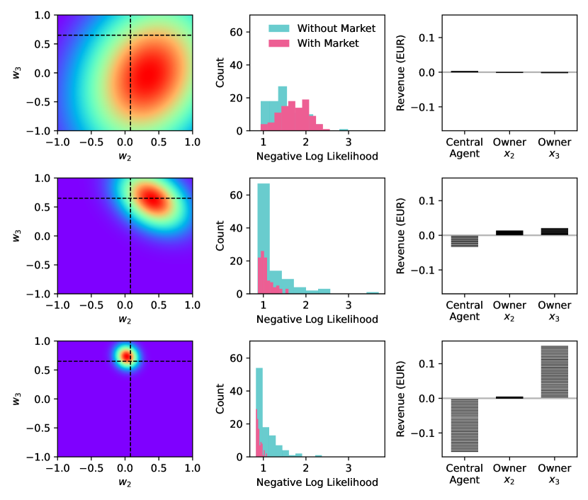
(a) Posterior Updates

(b) Predictive Performance

(c) Revenue

Figure 2: In-sample market with increasing batch size. The dashed lines in (a) highlight the true coefficient values. The histogram in (b) shows the in-sample NLL distribution. The horizontal bars in (c) are the cumulative revenues given the value of each datapoint provided.

4.2 Uncertainty Quantification

Next we illustrate our four considered setups, highlighting the benefit to the central agent of merely facilitating Bayesian regression analyses. We set the true parameters to $\textbf{w}=[-0.1,0.3,0.8,-0.4]^{\top}$ and $\xi_{Y_{t}}=0.5,\,\forall t$. We again emulate batch inference and run a Monte-Carlo simulation whereby we clear the market $10^{3}$ times for several different sample sizes (i.e., numbers of in-sample observations) and record the expected NLL for $10^{3}$ out-of-sample observations for each. This is carried out using both maximum likelihood estimation and Bayesian regression analyses.Figure 3 shows the empirical average of the percentage improvement in the objective value for the Bayesian regression model. Observe that the improvement is most significant across all setups when the sample size is relatively small, as the additional piece of uncertainty in the parameter estimates plays a greater role in the predictive distribution, increasing the predictive likelihood. Then, as the sample size increases, the parameter estimates converge in accordance with 13. Furthermore, as the additional layers of complexity are introduced, the benefit of incorporating parameter uncertainty increases considerably. These improvements attained by converting to a Bayesian framework indicate a better calibration of uncertainty, enriching the information used by the central agent for risk-informed decision-making downstream.

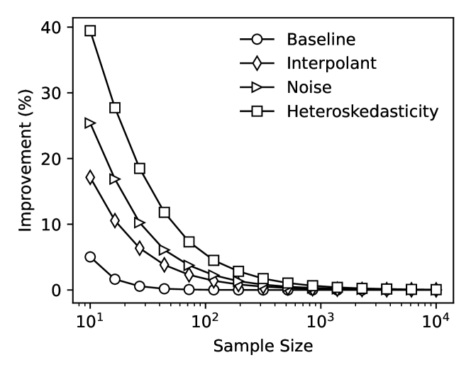
Figure 3: Empirical average of the percentage improvement in the NLL ratio for BLR relative to MLE, plotted as a function of sample size.

4.3 Convergence Analysis

Now we present an empirical study of the in-sample asymptotic convergence for our various market designs. Let the true coefficeints and noise precision be given by $\textbf{w}=[-0.1,0.8,0.7,-0.9]^{\top}$ and $\xi_{Y_{t}}=1.0,\,\forall t$, respectively, focusing here solely on the Baseline setup, since asymptotic convergence is irrespective of the true data generating processes, but rather the set of modelling assumptions. A similar Monte-Carlo simulation is performed, recording the in-sample Shapley values for each run, the results of which are presented in Figure 4.

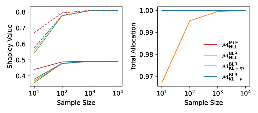
(a) Contributions

(b) Allocations

Figure 4: Empirical average of (a) expected Shapley values and (b) the expected total allocation, for each market design, plotted as a function of sample size. Dashed and solid lines in (a) correspond to features $x_{2,t}$ and $x_{3,t}$, respectively. In (b), the red and green lines are hidden behind the blue line, given budget balance is a universally held property in each of these markets.

Looking first at Figure 4(a), we see that with a small sample size, the frequentist market design assigns a larger contribution to the features compared with those using Bayesian regression, however these values indeed converge asymptotically in align with the theory. This discrepancy is likely due to the greater reduction in the in-sample objective provided by the maximum likelihood estimate, which is of course prone to overfitting. In Figure 4(b), we see that although the $\mathcal{M}^{\mathrm{BLR}}_{\mathrm{KL}-v}$ market yields a total allocation (i.e., the sum of the Shapley values divided by the value of the grand coalition) analogous to the likelihood-based markets, the $\mathcal{M}^{\mathrm{BLR}}_{\mathrm{KL}-m}$ market renders a surplus in revenue when the sample size is small. This demonstrates the trade-off incurred by virtue of the now universally held individual rationality property, in other words, budget balance is no longer guaranteed, even during the in-sample stage. That being said, this problem indeed resolves with increasing number of observations as the Shapley values converge.

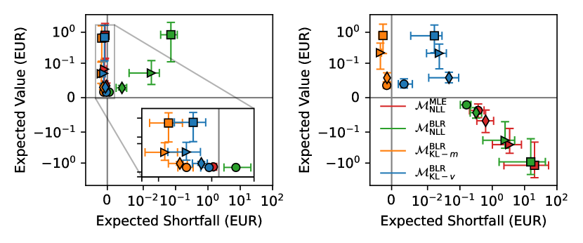
(a) In-sample

(b) Out-of-sample

Figure 5: Two-sided confidence intervals with a 95% confidence level for both the expected value and expected shortfall of the revenue received by the owner of $x_{2,t}$, with quantile parameter $\alpha=0.05$, for each setup, namely Baseline ($\circ$), Interpolant ($\diamond$), Noise ($\triangleright$) and Heteroskedasticity ($\square$).

4.4 Risk Exposure

We now turn our attention to the finances of the support agents, which we assess by computing both the expected value of the revenue, $\int\pi_{a,t}p(\pi_{a,t})\,d\pi_{a,t},\,\forall t$, and the expected shortfall (i.e., conditional value at risk), $-1/\alpha\int_{\pi_{a,t}\leq q_{\alpha}(\pi_{a,t})}\pi_{a,t}p(\pi_{a,t})\,d\pi_{a,t},\,\forall t$, for all $a\in\mathcal{A}_{-c}$, where $q_{\alpha}(\cdot)$ is the quantile with nominal level $\alpha$. We present empirical estimations of these values for a case study where we again clear the market for a new sample of data $10^{3}$ times and record the revenue of each support agent, with the true coefficients set to $\textbf{w}=[0.1,-0.5,0.0,0.7]^{\top}$, with noise precision $\xi_{Y_{t}}=0.67,\,\forall t$. We additionally set $\lambda=0.03$ EUR per time step and per unit improvement in $\ell$ for the both in-sample and out-of-sample stages. We use a simple sub-sampling method to derive the corresponding two-sided confidence intervals of both the expected value and expected shortfall of the revenue with a 95% confidence level. We run this simulation for each market design, as well as for each of the misspecification setups, with $10^{3}$ in-sample and out-of-sample observations. In Figure 5, we plot the revenue of the support agent who owns $x_{2,t}$. Considering first Figure 5(a), observe that the expected value of the revenue is relatively consistent across all market designs for each setup. However, for each additional layer of complexity, the expected shortfall is positive for the $\mathcal{M}^{\mathrm{BLR}}_{\mathrm{NLL}}$ market, increasing by almost two orders of magnitude in the latter setups. For the market designs based on the KL divergence, the expected shortfall remains somewhat constant around zero, highlighting the sizeable reductions in risk exposure possible by using the KL divergence instead of the NLL to allocate revenue. As we saw previously, the $\mathcal{M}^{\mathrm{MLE}}_{\mathrm{NLL}}$ market design seemingly performs better than its Bayesian counterpart during the in-sample stage. However, if we look now at Figure 5(b), we see this indeed does not generalize out-of-sample. For this small number of observations, the estimated moments of the posterior distribution are more likely to be sub-optimal, and hence the predictive likelihood is more volatile. In consequence, even the expected value of the out-of-sample revenue becomes more negative with each additional layer of complexity for the likelihood-based market designs, meaning that the individual rationality property is violated even in expectation. The out-of-sample revenues in the $\mathcal{M}^{\mathrm{MLE}}_{\mathrm{NLL}}$ market are now worse than for $\mathcal{M}^{\mathrm{BLR}}_{\mathrm{NLL}}$, demonstrating that the superior performance of the $\mathcal{M}^{\mathrm{MLE}}_{\mathrm{NLL}}$ market in-sample was indeed simply a result of overfitting. In contrast, the expected value of the revenue is relatively consistent with those in-sample for both KL divergence-based markets. Considering the risk, the expected shortfall for $\mathcal{M}^{\mathrm{BLR}}_{\mathrm{NLL}}$ and $\mathcal{M}^{\mathrm{MLE}}_{\mathrm{NLL}}$ increased by several orders of magnitude at the out-of-sample stage. Interestingly, one can now observe the consequence of re-instating budget balance by re-defining the characteristic function instead of the marginal contribution. Specifically, whilst for the $\mathcal{M}^{\mathrm{BLR}}_{\mathrm{KL}-m}$ market design, individual rationality is held universally, the expected shortfall in $\mathcal{M}^{\mathrm{BLR}}_{\mathrm{KL}-v}$ has drifted positive. That being said, the risks are generally considerably less compared with $\mathcal{M}^{\mathrm{BLR}}_{\mathrm{NLL}}$, suggesting that there is still merit to this approach if budget balance is essential.

4.4.1 Sensitivity Analysis: Sample Size

Using the same experimental procedure, we now consider the sensitivity of these findings to the number of in-sample observations, the results of which are shown in Figure 6. Note, the volumetric revenues are normalized here to account for the different sample sizes. In general, both the expected value and the expected shortfall of the revenue converge for all market designs. This was expected given the asymptotic convergence of the Shapley values shown previously. However, what is of note here is that out-of-sample, the expected shortfall associated with the likelihood-based market design takes considerably longer to converge, with substantial risk levels even for the larger sample sizes, notwithstanding that is merely the Baseline setup. This emphasizes that although the majority of the risk exposure manifests in the out-of-sample market stage, using the KL divergence to allocate revenue can help mitigate this significantly.

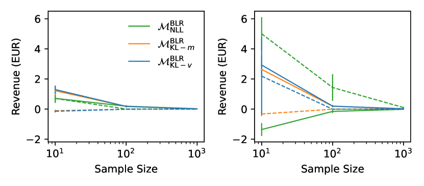
(a) In-sample

(b) Out-of-sample

Figure 6: Two-sided confidence intervals with 95% confidence level for both the expected returns (solid lines) and expected shortfall (dashed lines), with quantile parameter $\alpha=0.05$, for the first support agent considering the Baseline setup and plotted as a function of sample size.

4.4.2 Sensitivity Analysis: Coefficient Magnitude

We now consider the sensitivity to the magnitude of the true coefficient associated with the feature owned by the first support agent, by re-running the simluation with different values for $w_{2}$, all the while keeping the remaining coefficients constant. The results are shown in Figure 7. Still we see a lesser degree of inconsistency between the in-sample and out-of-sample payments for the market designs based on the KL divergence, both in terms of expected returns and risk, with considerably greater financial risk for $\mathcal{M}^{\mathrm{BLR}}_{\mathrm{NLL}}$ during the out-of-sample stage. We emphasize again that this is even for the simple Baseline setup. We also see that for each of the market designs, the expected value and the expected shortfall of the revenue appear quadratic in $|w_{2}|$. In fact, this should be of no surprise — given Assumptions 3 and 4, one can readily show that in a Bayesian framework, both the expected value and variance of the Shapley value for a feature are a quadratic function of its contribution to the prediction (Falconer et al., 2023). To be self-contained, we provide a proof in Appendix E. One could argue this to have fairness implications, since in theory more informative features are exposed to a greater extent of financial uncertainty, however this is out-of-scope and we hereby leave a more thorough exploration of this phenomenon as future work. In addition, we note that since this would allow us to analytically describe the expected shortfall, having more consistent results between stages, such as with the KL divergence market designs, could enable us to provide the support agents with a qualitative a priori upper bound on the risk (i.e., before clearing the market), even out-of-sample.

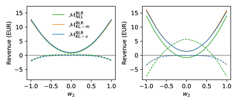
(a) In-sample

(b) Out-of-sample

Figure 7: Expected returns (solid lines) and expected shortfall (dashed lines), with quantile parameter $\alpha=0.05$, for the first support agent considering the Baseline setup and plotted as a function of $w_{2}$.

4.5 Nonstationary Processes

Until this point, we have assumed only batch inference (i.e., $\tau=1$), however in Section 2.3 we showed theoretically that this is merely a specification of the more general online Bayesian inference problem, which facilitates time-varying posterior moments. For the final simulation-based case study, let us consider a nonstationary data generating process, wherein the parameters initially take on the values $\textbf{w}=[0.0,-0.2,0.1,0.3]^{\top}$, with noise precision $\xi_{Y_{t}}=0.98,\,\forall t$. For simplicity, we only let the coefficient associated with $x_{2,t}$ vary with time, with the rest constant. To illustrate the effect of likelihood flattening, we consider two cases, where: (i) $w_{2}$ decreases linearly, and (ii) $w_{2}$ exhibits a discontinuity, each representing increasingly complex processes to capture, with respect to their stationary analogue. We carry out a Monte-Carlo simulation whereby we record the empirical average of the parameter estimates at each time step with various values for $\tau$, the results of which are presented in Figure 8. Of course, for the previous time-invariant cases, there would be no advantage of using likelihood flattening since the coefficients are stationary. For the more complex cases, as $\tau\mapsto 1$, our posterior beliefs decay more gradually, but as $\tau$ is reduced, we are able to better track the coefficient values, albeit with increased variance due to the fact that more weight is given to the flat prior.

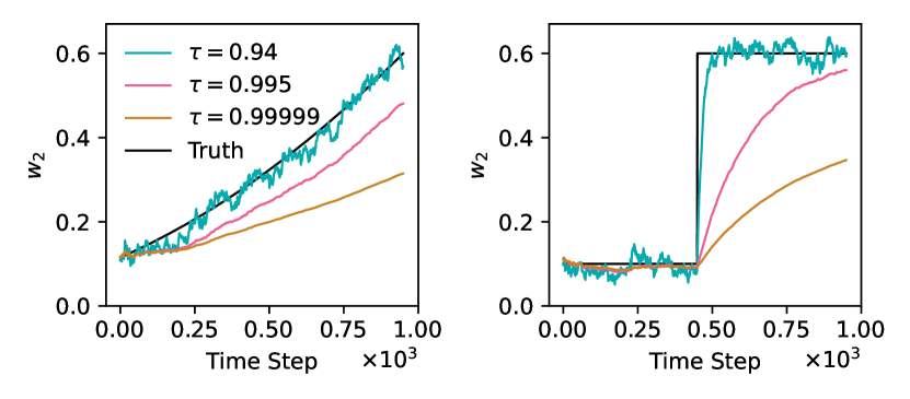
(a) Smooth

(b) Discontinuous

Figure 8: Temporal evolution of the empirical average of the estimated value for $w_{2}$. The estimates for the remaining parameters are omitted for clarity.

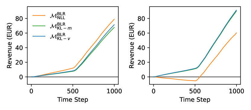
(a) In-sample

(b) Out-of-sample

Figure 9: Cumulative empirical averages of the expected value of the revenue, with quantile parameter $\alpha=0.05$, for the first support agent considering the Baseline setup.

As the discontinuity in Figure 8(b) represents a more extreme case of the smooth temporal evolution in Figure 8(a), we use this as a case study for further analysis. We run a Monte-Carlo simulation whereby we fix $\tau=0.94$ in order to better track the coefficient, albeit at the expense of increased variance. We re-run the entire online market clearing procedure $10^{3}$ times, each time tracking the temporal evolution of market revenue over $10^{3}$ time steps. We set $\lambda=0.95$ EUR per time step and per unit improvement in $\ell$ for both stages. Again, we carry out this simulation for each of the proposed Bayesian regression market designs, considering only the Baseline setup, the results of which are shown in Figure 9. Given the use of likelihood flattening, each of the market designs are able to capture the step-change in the true coefficient value. However, the extent of likelihood flattening required reduces the effective window size of observations, emulating a consistently small sample size even as more observations arrive. As a result, the likelhood-based market exhibits poor generalization to the out-of-sample stage as we have seen before. In fact, even though the true coefficient is $w_{2}=0.1$ before the step change, the expected value of the revenue is less than $0$, resulting in a negative cumulative revenue in the first half of the simulation, and hence overall the agent earns considerably less in this market. In contrast, we see that both the expected value and expected shortfall of the revenue in both $\mathcal{M}^{\mathrm{BLR}}_{\mathrm{KL}-m}$ and $\mathcal{M}^{\mathrm{BLR}}_{\mathrm{KL}-v}$ markets remain relatively consistent to those observed in-sample.

5 Real-world Application

We round off our experimental analysis by verifying the applicability of our proposal to real-world applications. We make use of an open source dataset, namely the Pan-European Climate Database, as detailed in Koivisto and Leon (2022). This dataset consists of hourly average solar irradiance values by country in Europe, obtained by simulating the output from south-facing solar photovoltaic (PV) modules across several intra-country regions, using meteorological data. Although this data is not exactly real, it effectively captures the spatio-temporal aspects of solar irradiance across the continent, with the benefit of not being contaminated with any spurious data points, as can often be the case with real-world datasets. Suppose that the electricity system operator in each country seeks to forecast its own country’s average generation from solar PV modules, with a view to subsequently estimate electricity demand and determine balancing resource requirements. For illustration, we consider six countries, namely United Kingdom (UK), Belgium (FR), Austria (AT), Greece (GR), Cyprus (CY) and Turkey (TR), each of which is assumed to enter the regression market to enhance their respective forecasts. For simplicity, we focus on a 1-hour forecasting horizon (i.e., nowcasting) using only linear basis functions, though both longer latency periods and more complex models could be considered. We extract data that spans a two-year period from the start of 2018 to the end of 2019, with an hourly resolution. Suppose that each of the six countries takes turn in assuming the role of either the central agent in parallel transactions. We use a simple Auto-Regressive with eXogenous input model with a maximum of one lag for each feature. For solar energy, forecasting with lags simultaneously captures temporal correlations at particular locations and any indirect spatial correlations between neighboring locations, resulting from the natural development of cloud coverage and the rotation of the sun. We present the rolling average of the raw irradiance values in Figure 10(a), which highlights the seasonality of generation from solar PV modules, peaking during the summer months as expected. Similarly, by plotting the hourly average irradiance in Figure 10(b), one can observe the spatial correlations such that at any given time, the actual generation in the more Easterly countries could be indicative of what is to come in Western Europe later in the day.

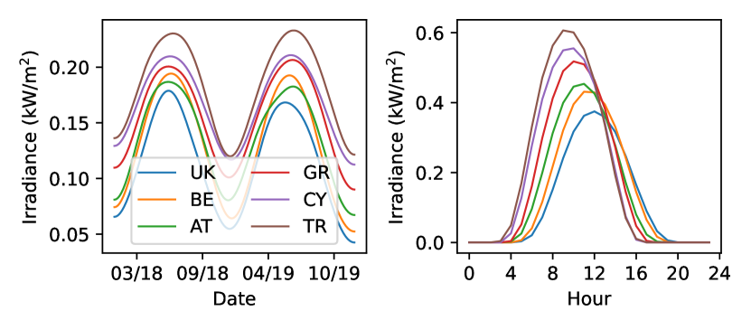
(a) Rolling Average

(b) Hourly Average

Figure 10: The rolling average and hourly average solar irradiance observed in each country during the two-year time period of 2018–2019.

For each forecast, we model the likelihood as an independent Gaussian stochastic process with finite precision, similar to the framework described in Section 4. We consider an online setting such that over the entire two-year period, at each time step (i.e., one hour interval), when a new observation of the target signal is collected, the forecast issued at the previous time step is used for out-of-sample market clearing, whilst at the same time, the posterior is updated and the in-sample market is cleared, and a forecast for the next time step is subsequently made. We set $\tau=0.998$ and assume the valuation of each central agent to be $\lambda=50$ EUR and $\lambda=150$ EUR per time step and per unit improvement in $\ell$ for the in-sample and out-of-sample stages, respectively, to reflect the costs of balancing resources. With each country set as the central agent, we record the predictive performance and cumulative revenues of the remaining countries across both stages over the entire two-year span using the $\mathcal{M}^{\mathrm{BLR}}_{\mathrm{KL}-v}$ market design. Let us first consider the improvements in predictive performance with respect to the NLL exhibited by each of the countries when assuming the role of the central agent. We show the average quarterly results in Table 2. In general, we observe a seasonality in the objective equivalent to that of the irradiance itself, such that smaller enhancements in predictive performance are exhibited during the end two quarters, since there is less potential for improving predictive performance when irradiance is low. Both United Kingdom and Greece receive the greatest improvements, with Cyprus and Turkey the smallest, the latter of which is likely due to the fact that these countries are further East, thus less able to exploit the spatial correlations depicted in Figure 10(b). We also note that the distribution of performance improvements amongst the countries is fairly similar between the in-sample and out-of-sample stages, which suggests any nonstationarities, as well as the time-varying objective estimates, are smooth, and hence the in-sample posterior is a relatively efficient estimator for use out-of-sample in the next time step.

Country	In-sample				Out-of-sample
	Q1	Q2	Q3	Q4	Q1	Q2	Q3	Q4
UK	$0.40$	$2.24$	$2.24$	$0.37$	$0.39$	$2.32$	$2.45$	$0.36$
BE	$0.34$	$1.58$	$1.59$	$0.51$	$0.33$	$1.60$	$1.61$	$0.50$
AT	$0.66$	$1.77$	$1.47$	$0.72$	$0.65$	$1.81$	$1.49$	$0.72$
GR	$0.73$	$2.11$	$2.40$	$0.82$	$0.74$	$2.15$	$2.44$	$0.81$
CY	$0.44$	$1.05$	$1.20$	$0.56$	$0.43$	$1.05$	$1.21$	$0.55$
TR	$0.43$	$1.00$	$1.35$	$0.65$	$0.42$	$1.00$	$1.36$	$0.64$

Table 2: Fractional improvement in the NLL ratio as a result of participating in the regression market, averaged over each calendar quarter, for both in-sample and out-of-sample market stages.

In Figure 11, we present the smoothed evolution of the revenues across both the in-sample and out-of-sample market stages. We see that, similar to the objective estimates, the allocation is by no means constant with time, such that the revenues of each agent are typically lower over the winter months and increase throughout the rest of the year. The value of each observation therefore also reflects the seasonality observed in the generation from solar PV modules. We also see the spatio-temporal dynamics of solar irradiance, as countries to the East of the central agent, particularly those nearby or with high nominal generation, contribute most to the uplift. The revenues received by the remaining countries when either Cyprus or Turkey assume the role of the central agent are relatively small, in accordance with the results in Table 2. Lastly, we note that the revenues earned by some of the countries over the entire two-year period are substantial, for instance with Greece as the central agent, the system operator in Cyprus earns approximately $1.2\times 10^{6}$ EUR, representing an average unit value of around $70$ EUR per observation shared.

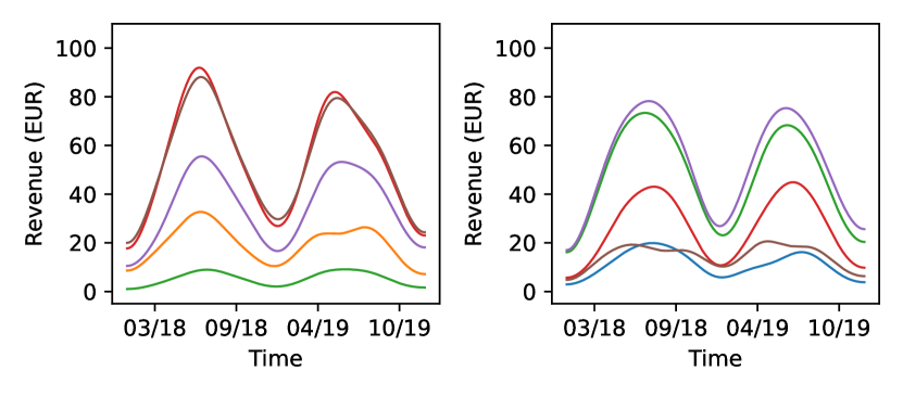
(a) UK

(b) BE

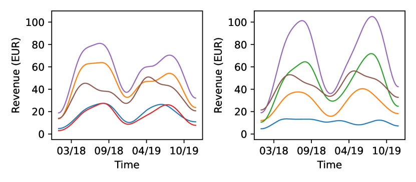
(c) AT

(d) GR

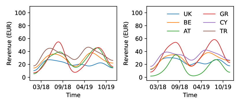
(e) CY

(f) TR

Figure 11: Smoothed evolution of total revenue per time step made by each of the six countries to the remaining five whilst assuming the role of the central agent.

6 Conclusions

Data-driven firms that employ predictive analytics (e.g., machine learning) often lack access to adequate sources of data. Whilst sharing data amongst others could bring potential advantages, many firms remain hesitant to do so, predominantly due to privacy concerns and the fear of losing a competitive edge, rather than the practical complexities involved in establishing data-sharing pipelines. Analytics markets, or in our case regression markets, offer a possible solution to this, wherein data is commoditized with respect to the particular analytics task at hand, providing incentives for information exchange through remuneration. In this paper, we proposed a mechanism design for a regression market that facilitates a generalized approach to forecasting, one based on Bayesian regression analyses. As a result, we provide the buyer with richer and more nuanced information about future outcomes, offering better calibration of uncertainty to be used for risk-informed decision-making downstream. We first introduced what we posed as the Bayesian analogue of recent frequentist-based proposals, but showed that this market design, akin to those in current literature, exposes the buyer to considerable financial risks, especially when a limited number of observations are available or when the data generating processes are nonstationary. In these settings, sub-optimal estimates of the posterior distribution led to sizeable expected losses, especially during the out-of-sample market stage, for which the in-sample estimates of the posterior moments are less efficient. To mitigate these risks, we posed to re-formulate the value of a feature in terms of the information gain it provides. In particular, we derived two alternative definitions of the marginal contribution of a feature towards a set of other features using the Kullback–Leibler divergence, the first of which could guarentee individual rationality universally (i.e., no support agents would be allocated negative revenue). However, there is of course no free lunch, as this was at the expense of budget balance. Nevertheless, we showed that in both cases using the KL divergence was able to provide more robust revenue allocations by alleviate the financial risks that the support agents were exposed to, even at the out-of-sample market stage. Possible directions for direct future work could include extending the concepts of our proposal to a broader class of machine learning models, such as (i) non-convex regression, which will have implications on market property guarantees; (ii) non-Gaussian hypotheses, which may require approximation bounds; and lastly (iii) alternative modelling paradigms, for instance, classification, unsupervised learning, or data-driven optimization problems in general. On a broader note, there are still many unanswered questions in relation to the complexities of treating data as a commodity. For instance, in practice, datasets cover different spatial and temporal horizons, and may become (un-)available to the market at different times. Accordingly, aggregating real-world datasets in an online fashion may not be straightforward and may require revision of fundamental concepts in online learning and mechanism design. Additionally, much of the current literature relies on the assumption that the valuation of the central agent is both linear and easily conceivable with respect of the objective function, which may not be true if the downstream decision-making process is complex or in the face of externalities (e.g., whether or not competing firms also get access to the data may affect the valuation). Support agents may also have reservations to share their information, for instance due to privacy concerns or conflicts of interest. This, as well as physical costs of collecting and storing data, may require a minimum revenue to be obtained. Lastly, if firms that share data are indeed competitors in a downstream market, one may be interested in if, by providing better use of information, the analytics market is beneficial to social welfare, and if those that lose competitive advantage by sharing their information are adequately compensated.

Appendix A Truthfulness Property (Theorem 2)

We provide a proof of the truthfulness property provided by Theorem 2, which describes the asymptotic market properties. We model the target signal, $\{Y_{t}\}$, as a deviation from the deterministic linear interpolant in (2) under the following centred additive noise process

$$p(\mathcal{D}_{\mathcal{C},t}|\Theta_{\mathcal{C}})=\prod_{t^{\prime}\leq t}\mathcal{N}(f(\textbf{x}_{\mathcal{C},t},\textbf{w}_{\mathcal{C}}),\xi_{Y_{t}}^{-1}),\quad\forall t.$$ (16)

Without loss of generality, consider $\xi_{Y_{t}}=\xi,\forall t$ to be a hyperparameter, such that the parameters to be inferred from data are only the regression coefficients (i.e., $\Theta_{\mathcal{C}}=\{\textbf{w}_{\mathcal{C}}\}$). As the prior is assumed to be uninformative, we avoid imposing any specific assumptions or biases on the parameter estimate. Accordingly, we set the conjugate prior to be a zero-mean isotropic Gaussian distribution with infinitely broad variance, that is, $p(\textbf{w}_{\mathcal{C}}|\xi)=\mathcal{N}(\textbf{0},\gamma^{-1}\textbf{I})$ with $\gamma\mapsto 0$ and $\textbf{I}\in\mathbb{R}^{|\mathcal{C}|\times|\mathcal{C}|}$ is the identity matrix. Let $\textbf{m}_{\mathcal{C},t}\in\mathbb{R}^{|\mathcal{C}|}$ and $\textbf{K}_{\mathcal{C},t}\in\mathbb{R}^{|\mathcal{C}|\times|\mathcal{C}|}$ denote the mean vector and the covariance matrix of the posterior at a particular time step $t$, respectively. As the posterior is Gaussian, we indeed know that its mode coincides with its mean, and since we can write the logarithm of the posterior as the sum of both the logarithm of the likelihood and the logarithm of the prior, the posterior mean reduces to the maximum likelihood estimate, given by

$$\hat{\textbf{m}}_{\mathcal{C},t} =\operatorname*{argmax}_{\textbf{w}_{\mathcal{C}}}\ \log\left(p(\mathcal{D}_{\mathcal{C},t}|\textbf{w}_{\mathcal{C}},\xi)\right)+\log\left(p(\textbf{w}_{\mathcal{C}}|\xi)\right),\quad\forall t,$$ (17a)

$$=\mathop{\mathrm{argmin}}_{\textbf{w}_{\mathcal{C}}}\ \sum_{t^{\prime}\leq t}(y_{t^{\prime}}-f(\textbf{x}_{\mathcal{C},t^{\prime}},\textbf{w}_{\mathcal{C}}))^{2},\quad\forall t,$$ (17b)

as would the estimated noise precision if inferred from data. Now suppose the data for one or more of the features is reported untruthfully, such that for any particular time step $t$, the vector of features is, $\tilde{\textbf{x}}_{t}=\textbf{x}_{t}+\boldsymbol{\eta}_{t}$, where $p(\boldsymbol{\eta}_{t})=\mathcal{N}(\boldsymbol{0},\boldsymbol{\Sigma})$. The covariance matrix $\boldsymbol{\Sigma}$ is diagonal, the elements of which corresponding to truthfully reported features are zero, such that only untruthful features are subject to noise. For brevity, and without loss of generality, we consider only the set of linear basis functions. Substituting the new feature vector into the linear interpolant, the optimization problem in (17b) is augmented to minimize the expected sum-of-squares error, where the expectation is taken over the random noise,

$$\hat{\textbf{m}}_{\mathcal{C},t} =\mathop{\mathrm{argmin}}_{\textbf{w}_{\mathcal{C}}}\ \mathbb{E}\,\left[\sum_{t^{\prime}\leq t}\left(y_{t^{\prime}}-f(\tilde{\textbf{x}}_{\mathcal{C},t^{\prime}},\textbf{w}_{\mathcal{C}})\right)^{2}\right],\quad\forall t,$$ (18a)

$$=\mathop{\mathrm{argmin}}_{\textbf{w}_{\mathcal{C}}}\ \sum_{t^{\prime}\leq t}\left((y_{t^{\prime}}-\textbf{w}_{\mathcal{C}}^{\top}\textbf{x}_{\mathcal{C},t^{\prime}})^{2}-2\textbf{w}_{\mathcal{C}}^{\top}\mathbb{E}\left[\boldsymbol{\eta}_{\mathcal{C},t^{\prime}}\right](y_{t^{\prime}}-\textbf{w}_{\mathcal{C}}^{\top}\textbf{x}_{\mathcal{C},t^{\prime}})+\textbf{w}_{\mathcal{C}}^{\top}\mathbb{E}\left[\boldsymbol{\eta}_{\mathcal{C},t^{\prime}}\boldsymbol{\eta}_{\mathcal{C},t^{\prime}}^{\top}\right]\textbf{w}_{\mathcal{C}}\right),\ \ \forall t,$$ (18b)

$$=\mathop{\mathrm{argmin}}_{\textbf{w}_{\mathcal{C}}}\ \sum_{t^{\prime}\leq t}\left(y_{t^{\prime}}-\textbf{w}_{\mathcal{C}}^{\top}\textbf{x}_{\mathcal{C},t}\right)^{2}+\textbf{w}_{\mathcal{C}}^{\top}\boldsymbol{\Sigma}\textbf{w}_{\mathcal{C}},\quad\forall t,$$ (18c)

where (18c) is derived from (18b) by recalling that $\mathbb{E}[\boldsymbol{\eta}_{t}]=\boldsymbol{0}$ and hence $\mathbb{E}[\boldsymbol{\eta}_{t}\boldsymbol{\eta}_{t}^{\top}]=\boldsymbol{\Sigma}$. For the special case whereby equal noise is added to all features, such that $\boldsymbol{\Sigma}=\beta\mathbf{I}$, for some constant $\beta$, the second term in (18c) reduces to $\textbf{w}_{\mathcal{C}}^{\top}\boldsymbol{\Sigma}\textbf{w}_{\mathcal{C}}=\beta||\textbf{w}_{\mathcal{C}}||^{2}_{2}$, which results in a vector of coefficient analogous to that obtained using Ridge regression, with shrinkage penalty $\beta=\gamma/\xi$. Moreover, since $\boldsymbol{\Sigma}$ is a diagonal matrix, agents are not able to behave spitefully by adding noise to their features in effort to reduce the payments of others. In general though, we observe that the likelihood is maximized as $\gamma\mapsto 0$, hence any addition of noise will reduce the predictive likelihood, and subsequently the payments, given the definition in (11), thereby completing the proof.

Appendix B Proof of Corollary 4

Lemma B.1

The difference between the expected value of the quadratic loss of two maximum likelihood linear regression models, both with a Gaussian likelihood function, is equivalent to the expected squared difference in their interpolated functions.

Proof [Lemma B.1] In a maximum likelihood linear regression setting with a Gaussian likelihood, the objective is proportional to the expected value of the quadratic loss which we can decompose as follows:

$$\mathbb{E}\,\left[\left(f_{\mathcal{C},t}-y_{t}\right)^{2}\right] =var\left(f_{\mathcal{C},t}-y_{t}\right)+\mathbb{E}\left[f_{\mathcal{C},t}-y_{t}\right]^{2},$$ (19a)

$$=var\left(f_{\mathcal{C},t}\right)+var\left(y_{t}\right)-2\,cov\left(f_{\mathcal{C},t},y_{t}\right),$$ (19b)

$$=var\left(y_{t}\right)-var\left(f_{\mathcal{C},t}\right).$$ (19c)

where for brevity, we write $f_{\mathcal{C},t}=f(\mathbf{x}_{\mathcal{C},t},\mathbf{w}_{\mathcal{C}}),\ \forall t$. We can write the expression in (19c) since the covariance between the prediction and the target is equal to the variance of the prediction itself since the estimators are unbiased. If we let $\mathcal{C}_{i}=\mathcal{C}\cup\{i\}$ denote the addition of the $i$-th feature index to a particular coalition for all $C\subseteq\mathcal{I}_{-c}$, we get that

$$\mathbb{E}\,\left[\left(f_{\mathcal{C},t}-y_{t}\right)^{2}\right]-\mathbb{E}\,\left[\left(f_{\mathcal{C}_{i},t}-y_{t}\right)^{2}\right] =var\left(f_{\mathcal{C}_{i},t}\right)-var\left(f_{\mathcal{C},t}\right),$$ (20a)

$$=\mathbb{E}\left[\left(f_{\mathcal{C}_{i},t}\right)^{2}\right]-\mathbb{E}\left[f_{\mathcal{C}_{i},t}\right]^{2}-\mathbb{E}\left[\left(f_{\mathcal{C},t}\right)^{2}\right]+\mathbb{E}\left[f_{\mathcal{C},t}\right]^{2},$$ (20b)

$$=\mathbb{E}\left[\left(f_{\mathcal{C}_{i},t}\right)^{2}\right]-\mathbb{E}\left[\left(f_{\mathcal{C},t}\right)^{2}\right],$$ (20c)

$$=\mathbb{E}\left[\left(f_{\mathcal{C}_{i},t}\right)^{2}\right]+\mathbb{E}\left[\left(f_{\mathcal{C},t}\right)^{2}\right]-2\mathbb{E}\left[\left(f_{\mathcal{C},t}\right)^{2}\right],$$ (20d)

$$=\mathbb{E}\left[\left(f_{\mathcal{C}_{i},t}\right)^{2}\right]+\mathbb{E}\left[\left(f_{\mathcal{C},t}\right)^{2}\right]-2\left(var\left(f_{\mathcal{C}_{i},t}\right)+\mathbb{E}\left[f_{\mathcal{C}_{i},t}\right]^{2}\right).$$ (20e)

Note that we can ignore the covariance $cov\left(f_{\mathcal{C},t},\left(f_{\mathcal{C}_{i},t}-f_{\mathcal{C},t}\right)\right)$ since the prediction is not correlated with the residuals. Hence, the variance term can be re-written as follows:

$$var\left(f_{\mathcal{C}_{i},t}\right) =var\left(f_{\mathcal{C},t}+\left(f_{\mathcal{C}_{i},t}-f_{\mathcal{C},t}\right)\right),$$ (21a)

$$=var\left(f_{\mathcal{C},t}\right)+var\left(f_{\mathcal{C}_{i},t}-f_{\mathcal{C},t}\right),$$ (21b)

$$=2var\left(f_{\mathcal{C},t}\right)+var\left(f_{\mathcal{C}_{i},t}\right)-2cov\left(f_{\mathcal{C}_{i},t},f_{\mathcal{C},t}\right),$$ (21c)

and we hence get that $var\left(f_{\mathcal{C},t}\right)=cov\left(f_{\mathcal{C}_{i},t},f_{\mathcal{C},t}\right)$. Given that upon standardization, $\mathbb{E}\left[f_{\mathcal{C},t}\right]=0$ and $\mathbb{E}\left[f_{\mathcal{C}_{i},t}\right]=0$, we can re-write the last term in (20e) as follows:

$$var\left(f_{\mathcal{C}_{i},t}\right)+\mathbb{E}\left[f_{\mathcal{C}_{i},t}\right]^{2} =cov\left(f_{\mathcal{C}_{i},t},f_{\mathcal{C}}\right)+\mathbb{E}\left[f_{\mathcal{C}_{i},t}\right]\mathbb{E}\left[f_{\mathcal{C},t}\right],$$ (22a)

$$=\mathbb{E}\left[f_{\mathcal{C}_{i},t}f_{\mathcal{C},t}\right].$$ (22b)

Therefore, the difference in expected values of the quadratic loss reduces to the following, which completes the proof:

$$\mathbb{E}\,\left[\left(f_{\mathcal{C},t}-y_{t}\right)^{2}\right]-\mathbb{E}\,\left[\left(f_{\mathcal{C}_{i},t}-y_{t}\right)^{2}\right] =\mathbb{E}\left[\left(f_{\mathcal{C}_{i},t}\right)^{2}\right]+\mathbb{E}\left[\left(f_{\mathcal{C},t}\right)^{2}\right]-2\mathbb{E}\left[f_{\mathcal{C}_{i},t}f_{\mathcal{C},t}\right],$$ (23a)

$$=\mathbb{E}\left[\left(f_{\mathcal{C}_{i},t}-f_{\mathcal{C},t}\right)^{2}\right].$$ (23b)

Lemma B.2

Under Assumption 4, the expected KL divergence between two predictive distributions is asymptotically equivalent to the expected difference in their predictive means.

Proof [Lemma B.2]. Following the notation as in Appendix A, we can write the general expression for the posterior predictive distribution in (6) as

$$p(y_{t}\,|\,\textbf{x}_{\mathcal{C},t})=\mathcal{N}(f(\textbf{x}_{\mathcal{C},t},\textbf{m}_{\mathcal{C},t}),\xi_{\mathcal{C},t}),\quad\forall t,$$ (24)

where $\xi_{\mathcal{C},t}$ is the precision (i.e., inverse variance) comprising the finite precision of the intrinsic noise and the uncertainty the coefficients such that, $1/\xi_{\mathcal{C},t}=1/\xi+\textbf{x}_{\mathcal{C},t}^{\top}\textbf{S}_{\mathcal{C},t}\textbf{x}_{\mathcal{C},t},\ \forall t$. Let $Z_{t}=Y_{t}-f_{\mathcal{C}_{d},t},\,\forall t$. Since the predictive distribution is a univariate Gaussian, the logarithm of the likelihood ratio can be written as follows:

$$\log\left(\frac{p(y_{t}\,|\,\textbf{x}_{\mathcal{C}_{i},t})}{p(y_{t}\,|\,\textbf{x}_{\mathcal{C},t})}\right) =\frac{1}{2}\left(\frac{\frac{\sqrt{\xi_{\mathcal{C},t}}}{\sqrt{2\pi}}\exp\left(\frac{1}{2}\xi_{\mathcal{C},t}(Y_{t}-f_{\mathcal{C},t})^{2}\right)}{\frac{\sqrt{\xi_{\mathcal{C}_{i},t}}}{\sqrt{2\pi}}\exp\left(\frac{1}{2}\xi_{\mathcal{C}_{i},t}(Y_{t}-f_{\mathcal{C}_{i},t})^{2}\right)}\right)$$ (25a)

$$=\frac{1}{2}\left(\log\left(\frac{\xi_{\mathcal{C}_{i},t}}{\xi_{\mathcal{C},t}}\right)-\xi_{\mathcal{C}_{i},t}(Y_{t}-f_{\mathcal{C}_{i},t})^{2}-\xi_{\mathcal{C},t}(Y_{t}-f_{\mathcal{C},t})^{2}\right),$$ (25b)

$$=\frac{1}{2}\log\left(\frac{\xi_{\mathcal{C}_{i},t}}{\xi_{\mathcal{C},t}}\right)-\frac{1}{2}(\xi_{\mathcal{C}_{i},t}-\xi_{\mathcal{C},t})Z_{t}^{2}-\xi_{\mathcal{C},t}\Delta_{f_{\mathcal{C}_{i},t}}Z_{t}+\frac{1}{2}\xi_{\mathcal{C},t}\left(\Delta_{f_{\mathcal{C}_{i},t}}\right)^{2},$$ (25c)

where the expression, $\Delta_{f_{\mathcal{C}_{i},t}}=f_{\mathcal{C},t}-f_{\mathcal{C}_{i},t},\ \forall t$, denotes the difference in means. The KL divergence is given by the expectation of (25c) with respect to the predictive distribution that includes the $i$-th feature. Whilst the expression is not linear in $Z_{t}$, recall that in general $\mathbb{E}[Z_{t}^{2}]\triangleq var\left[Z_{t}\right]+\mathbb{E}[Z_{t}]^{2}$. The variance and expected value, of $Z_{t}$ reduces to $var\left[Z_{t}\right]=var\left[Y_{t}-f_{\mathcal{C},t}\right]=1/\xi_{\mathcal{C},t}$ and $\mathbb{E}[Z_{t}]=\mathbb{E}[Y_{t}-f_{\mathcal{C}_{d},t}]=0$, respectively. Given (13), we get that $\xi_{\mathcal{C}_{i},t}\xrightarrow{\enskip t\enskip}\xi_{\mathcal{C},t}$, hence we can derive the KL divergence as follows, which completes the proof:

$$\mathbb{E}\left[D_{\textrm{KL}}\left(p(y_{t}|\textbf{x}_{\mathcal{C}_{i},t})||p(y_{t}|\textbf{x}_{\mathcal{C},t})\right)\right] =\mathbb{E}\,\left[\int_{Y_{t}}p(y_{t}\,|\,\textbf{x}_{\mathcal{C}_{i},t})\,\log\left\{\frac{p(y_{t}\,|\,\textbf{x}_{\mathcal{C}_{i},t})}{p(y_{t}\,|\,\textbf{x}_{\mathcal{C},t})}\right\}d{y_{t}}\right],$$ (26a)

$$=\mathbb{E}\,\left[\frac{1}{2}\left(\log\left\{\frac{\xi_{\mathcal{C}_{i},t}}{\xi_{\mathcal{C},t}}\right\}-1+\frac{\xi_{\mathcal{C},t}}{\xi_{\mathcal{C}_{i},t}}+\xi_{\mathcal{C},t}\Delta_{f_{\mathcal{C}_{i},t}}^{2}\right)\right],$$ (26b)

$$\xrightarrow{\enskip t\enskip}\frac{\xi}{2}\,\mathbb{E}\,\left[\left(f_{\mathcal{C}_{i},t}-f_{\mathcal{C},t}\right)^{2}\right],\ \mathrm{almost}\ \mathrm{surely}.$$ (26c)

Proof [Corollary 4]. The marginal contribution derived using the expected NLL is equivalent to that obtained using the quadratic loss, and hence given by an in-sample estimate of the following,

$$m_{t}(\{i\},\mathcal{C})=\frac{\xi^{2}}{2}\left(\mathbb{E}\,\left[\left(f_{\mathcal{C},t}-y_{t}\right)^{2}\right]-\mathbb{E}\,\left[\left(f_{\mathcal{C}_{i},t}-y_{t}\right)^{2}\right]\right).$$ (27)

Combining the results from Lemmas B.1 and B.2, we can see that $(\ref{eq:kl_redef_mc})\xrightarrow{\enskip t\enskip}(\ref{eq:mse_contribution})$, and therefore, since all other terms within the definition in (9) remain unchanged, the Shapley values, and therefore the payments, will converge, thereby completing the proof.

Appendix C Proof of Budget Balance Violation (Theorem 5)

We provide here a proof that budget balance is violated under the definition of marginal contribution in (14), as described in Theorem 5. Recall that budget balance proceeds from the semivalue axiom efficiency, which in our context translate to: the total attribution allocated to all features should sum to the value of the grand coalition, that is, $v_{t}(\mathcal{I}_{c})-v_{t}(\mathcal{I})=\sum_{i\in\mathcal{I}_{-c}}\phi_{i,t},\ \forall t$. Using (9) we can expand this definition to reveal the telescoping sum structure of the Shapley value such that

$$\sum_{i\in\mathcal{I}_{-c}}\phi_{i,t} =\sum_{i\in\mathcal{I}_{-c}}\sum_{\mathcal{C}\in\mathcal{P}(\mathcal{I}_{-c}\setminus\{i\})}\frac{|\mathcal{C}|!(|\mathcal{I}_{-c}|-|\mathcal{C}|-1)!}{|\mathcal{I}_{-c}|!}\,\left(\mathcal{C}^{\prime})-v_{t}(\mathcal{C}^{\prime}\cup\{i\})\right),\quad\forall t,$$ (28a)

$$=|\mathcal{I}_{-c}|\underbracket{\frac{0!(|\mathcal{I}_{-c}|-1)!}{|\mathcal{I}_{-c}|!}v_{t}(\mathcal{I}_{c})}_{\begin{subarray}{c}\textrm{The value of the {central agent}}\\ \textrm{coalition appears $|\mathcal{I}_{-c}|$}\\ \textrm{times.}\end{subarray}}-|\mathcal{I}_{-c}|\underbracket{\frac{(|\mathcal{I}_{-c}|-1)!1!}{|\mathcal{I}_{-c}|!}v_{t}(\mathcal{I})}_{\begin{subarray}{c}\textrm{The value of the {grand}}\\ \textrm{coalition appears $|\mathcal{I}_{-c}|$}\\ \textrm{times.}\end{subarray}}+$$

$$\sum_{\begin{subarray}{c}\mathcal{C}\in\mathcal{P}(\mathcal{I}_{-c})\\ \ \mathcal{C}\neq\emptyset\end{subarray}}(|\mathcal{I}_{-c}|-|\mathcal{C}|)\underbracket{\left(\frac{|\mathcal{C}|!(|\mathcal{I}_{-c}|-|\mathcal{C}|-1)!}{|\mathcal{I}_{-c}|!}\right)v_{t}(\mathcal{C}^{\prime})}_{\begin{subarray}{c}\textrm{The value of the coalition $\mathcal{C}$ appears}\\ \textrm{$|\mathcal{I}_{-c}|-|\mathcal{C}|$ times with a {positive}}\\ \textrm{sign, i.e., once per agent {in} $\mathcal{C}$.}\end{subarray}}-$$

$$\sum_{\begin{subarray}{c}\mathcal{C}\in\mathcal{P}(\mathcal{I}_{-c})\\ \ \mathcal{C}\neq\emptyset\end{subarray}}|\mathcal{C}|\underbracket{\left(\frac{(|\mathcal{C}|-1)!(|\mathcal{I}_{-c}|-|\mathcal{C}|)!}{|\mathcal{I}_{-c}|!}\right)v_{t}(\mathcal{C}^{\prime})}_{\begin{subarray}{c}\textrm{The value of the coalition $\mathcal{C}$ appears}\\ \textrm{$|\mathcal{C}|$ times with a {negative} sign, i.e.,}\\ \textrm{once per agent {not in} $\mathcal{C}$.}\end{subarray}},\quad\forall t,$$ (28b)

$$=v_{t}(\mathcal{I}_{)}-v_{t}(\mathcal{I}),\quad\forall t.$$ (28c)

However, if we replace the expression for the marginal contribution with the definition in (14), we can similarly derive an expression for the value of the grand coalition, given by

$$\sum_{i\in\mathcal{I}_{-c}}\phi_{i,t}=|\mathcal{I}_{-c}|\frac{(|\mathcal{I}_{-c}|-1)!}{|\mathcal{I}_{-c}|!}\,\mathbb{E}\left[D_{\textrm{KL}}\left(p(y_{t}|\textbf{x}_{\mathcal{I},t},\mathcal{D}_{\mathcal{I},t-1})||p(y_{t}|\textbf{x}_{\mathcal{I}_{c},t},\mathcal{D}_{\mathcal{I}_{c},t-1})\right)\right].$$ (29)

This, however, holds true if and only if the KL divergence satisfies the triangle inequality with equality. Yet, we know that statistical divergence metrics do not satisfy the triangle inequality, that is, for any probability densities, $X$, $Y$ and $Z$, we get that $D_{\textrm{KL}}(X||Z)\not\leq D_{\textrm{KL}}(X||Y)+D_{\textrm{KL}}(Y||Z)$. Hence, by contradiction we can prove that using the KL divergence in this manner violates the efficiency axiom, and subsequently budget balance cannot be guaranteed.

Appendix D Proof of Corollary 7

Proof [Corollary 7]. In (15), we re-defined the valuation of a coalition to incorporate the KL divergence as below, which in Appendix B, was shown to converge to,

$$v_{t}(\mathcal{C}) =\mathbb{E}\left[D_{\textrm{KL}}\left(p(y_{t}|\textbf{x}_{\mathcal{C},t})||p(y_{t}|\textbf{x}_{\mathcal{I}_{c},t})\right)\right],$$ (30a)

$$\xrightarrow{\enskip t\enskip}\frac{\xi^{2}}{2}\left(\mathbb{E}\,\left[\left(f_{\mathcal{I}_{c},t}-y_{t}\right)^{2}\right]-\mathbb{E}\,\left[\left(f_{\mathcal{C},t}-y_{t}\right)^{2}\right]\right),\,\mathrm{almost\ surely}.$$ (30b)

Therefore, the marginal contribution of a feature to a coalition converges to the following:

$$m_{t}(\{i\},\mathcal{C}) \xrightarrow{\enskip t\enskip}\frac{\xi^{2}}{2}\left(\mathbb{E}\,\left[\left(f_{\mathcal{I}_{c},t}-y_{t}\right)^{2}\right]-\mathbb{E}\,\left[\left(f_{\mathcal{C}_{i},t}-y_{t}\right)^{2}\right]-\mathbb{E}\,\left[\left(f_{\mathcal{I}_{c},t}-y_{t}\right)^{2}\right]-\mathbb{E}\,\left[\left(f_{\mathcal{C},t}-y_{t}\right)^{2}\right]\right),$$ (31a)

$$=\frac{\xi^{2}}{2}\left(\mathbb{E}\,\left[\left(f_{\mathcal{C},t}-y_{t}\right)^{2}\right]-\mathbb{E}\,\left[\left(f_{\mathcal{C}_{i},t}-y_{t}\right)^{2}\right]\right),$$ (31b)

$$=(\ref{eq:mse_contribution}).$$ (31c)

As in Appendix B, since all other terms within the definition in (9) remain unchanged, the Shapley values, and therefore the payments, will converge, thereby completing the proof.

Appendix E Shapley Value Distribution

We here prove the following theorem to justify the results shown in Figure 7.

Theorem 8

Under Assumption 4, both the expected value and variance of the Shapley value for the $i$-th feature in a Bayesian framework are a quadratic function of its contribution to the prediction, thereby completing the proof.

Lemma E.1

The Shapley value for each feature will follow a scaled noncentral Chi-squared distribution with one degree of freedom.

Proof [Lemma E.1] When considering decomposition of variance, it becomes apparent that the Shapley value associated with the $i$-th feature corresponds to the variance accounted for in the target signal [Owen and Prieur, 2017], such that $\phi_{i}=w_{i}^{2}\,var(X_{i})$. Following Assumption 4, the posterior is a Gaussian distribution, for which the square is given by a noncentral Chi-squared distribution with one degree of freedom. For a particular feature, we can hence write the probability density function of the distribution of the Shapley value in closed-form as

$$\frac{1}{var(X_{i})var(w_{i})}p(\phi_{i})=\sum_{k=0}^{\infty}\frac{e^{\eta/2}(\eta/2)^{k})}{k!}\chi^{2}(1+2k),\,\forall i,$$ (32)

Proof [Theorem 8] The distribution in Lemma E.1 is simply a Poisson-weighted mixture of central chi-squared distributions, $\chi^{2}(\cdot)$, with noncentrality $\eta=\mathbb{E}[w_{i}]^{2}/var(w_{i})$. Since the moment generating function for such a mixture is known, we can derive the first two moments of the Shapley value distribution, giving the following:

$$\mathbb{E}[\phi_{i}] =1+\eta,\quad\forall i.$$ (33a)

$$var(\phi_{i}) =2var(w_{i})\left(2\mathbb{E}[w_{i}]^{2}+var(w_{i})\right)\left(var(X_{i})\right)^{2},\quad\forall i.$$ (33b)

This implies that both the expected value and variance of the Shapley value for the $i$-th feature are a quadratic function of its contribution to the prediction, thereby completing the proof.

References

- Acemoglu et al. [2022] Daron Acemoglu, Ali Makhdoumi, Azarakhsh Malekian, and Asu Ozdaglar. Too much data: Prices and inefficiencies in data markets. American Economic Journal: Microeconomics, 14(4):218–256, 2022.
- Acquisti et al. [2016] Alessandro Acquisti, Curtis Taylor, and Liad Wagman. The economics of privacy. Journal of Economic Literature, 54(2):442–492, 2016.
- Agarwal et al. [2019] Anish Agarwal, Munther Dahleh, and Tuhin Sarkar. A marketplace for data: An algorithmic solution. In Proceedings of the 2019 ACM Conference on Economics and Computation, pages 701–726, 2019.
- Agarwal et al. [2020] Anish Agarwal, Munther Dahleh, Thibaut Horel, and Maryann Rui. Towards data auctions with externalities, 2020. URL https://arxiv.org/abs/2003.08345.
- Agussurja et al. [2022] Lucas Agussurja, Xinyi Xu, and Bryan Kian Hsiang Low. On the convergence of the shapley value in parametric Bayesian learning games. In Kamalika Chaudhuri, Stefanie Jegelka, Le Song, Csaba Szepesvari, Gang Niu, and Sivan Sabato, editors, Proceedings of the 39th International Conference on Machine Learning, volume 162 of Proceedings of Machine Learning Research, pages 180–196. PMLR, 17–23 Jul 2022.
- Bergemann and Bonatti [2019] Dirk Bergemann and Alessandro Bonatti. Markets for information: An introduction. Annual Review of Economics, 11(1):85–107, 2019.
- Cao et al. [2017] Xuanyu Cao, Yan Chen, and K. J. Ray Liu. Data trading with multiple owners, collectors, and users: An iterative auction mechanism. IEEE Transactions on Signal and Information Processing over Networks, 3(2):268–281, 2017.
- Chalkiadakis et al. [2011] Georgios Chalkiadakis, Edith Elkind, and Michael Wooldridge. Computational aspects of cooperative game theory. Synthesis Lectures on Artificial Intelligence and Machine Learning, 5(6):1–168, 2011.
- Chen et al. [2020] Hugh Chen, Joseph D Janizek, Scott Lundberg, and Su-In Lee. True to the model or true to the data?, 2020. URL https://arxiv.org/abs/2006.16234.
- Cong et al. [2022] Zicun Cong, Xuan Luo, Jian Pei, Feida Zhu, and Yong Zhang. Data pricing in machine learning pipelines. Knowledge and Information Systems, 64(16):1417–1455, 2022.
- Covert et al. [2020] Ian Covert, Scott M Lundberg, and Su-In Lee. Understanding global feature contributions with additive importance measures. Advances in Neural Information Processing Systems, 33:17212–17223, 2020.
- Covert et al. [2021] Ian C Covert, Scott Lundberg, and Su-In Lee. Explaining by removing: A unified framework for model explanation. The Journal of Machine Learning Research, 22(1):9477–9566, 2021.
- Cummings et al. [2015] Rachel Cummings, Stratis Ioannidis, and Katrina Ligett. Truthful linear regression. In Peter Grünwald, Elad Hazan, and Satyen Kale, editors, Proceedings of the 28th Conference on Learning Theory, pages 448–483, Paris, France, 2015.
- Dahleh et al. [2016] Munther A Dahleh, Alireza Tahbaz-Salehi, John N Tsitsiklis, and Spyros I Zoumpoulis. Coordination with local information. Operations Research, 64(3):622–637, 2016.
- Dekel et al. [2010] Ofer Dekel, Felix Fischer, and Ariel D. Procaccia. Incentive compatible regression learning. Journal of Computer and System Sciences, 76(8):759–777, 2010.
- Dubey et al. [1981] Pradeep Dubey, Abraham Neyman, and Robert James Weber. Value theory without efficiency. Mathematics of Operations Research, 6(1):122–128, 1981.
- Falconer et al. [2023] Thomas Falconer, Jalal Kazempour, and Pierre Pinson. Incentivizing data sharing for energy forecasting: Analytics markets with correlated data, 2023. URL https://arxiv.org/abs/2310.06000.
- Fong and Holmes [2020] Edwin Fong and Chris C Holmes. On the marginal likelihood and cross-validation. Biometrika, 107(2):489–496, 2020.
- Gal-Or [1985] Esther Gal-Or. Information sharing in oligopoly. Econometrica, 53(2):329–343, 1985.
- Ghorbani and Zou [2019] Amirata Ghorbani and James Zou. Data shapley: Equitable valuation of data for machine learning. In Kamalika Chaudhuri and Ruslan Salakhutdinov, editors, Proceedings of the 36th International Conference on Machine Learning, volume 97 of Proceedings of Machine Learning Research, pages 2242–2251. PMLR, 09–15 Jun 2019.
- Gneiting and Katzfuss [2014] Tilmann Gneiting and Matthias Katzfuss. Probabilistic forecasting. Annual Review of Statistics and Its Application, 1:125–151, 2014.
- Guyon and Elisseeff [2003] Isabelle Guyon and André Elisseeff. An introduction to variable and feature selection. Journal of Machine Learning Research, 3(1):1157–1182, 2003.
- Guyon and Elisseeff [2010] Isabelle Guyon and André Elisseeff. An efficient explanation of individual classifications using game theory. Journal of Machine Learning Research, 11(1):1–18, 2010.
- Han et al. [2022a] Dongge Han, Michael Wooldridge, Alex Rogers, Olga Ohrimenko, and Sebastian Tschiatschek. Replication robust payoff allocation in submodular cooperative games. IEEE Transactions on Artificial Intelligence, 2022a.
- Han et al. [2022b] Liyang Han, Pierre Pinson, and Jalal Kazempour. Trading data for wind power forecasting: A regression market with lasso regularization. Electric Power Systems Research, 212:108442, 2022b.
- Hoerl and Kennard [1970] Arthur E Hoerl and Robert W Kennard. Ridge regression: Biased estimation for nonorthogonal problems. Technometrics, 12(1):55–67, 1970.
- Janzing et al. [2020] Dominik Janzing, Lenon Minorics, and Patrick Bloebaum. Feature relevance quantification in explainable ai: A causal problem. In Silvia Chiappa and Roberto Calandra, editors, Proceedings of the Twenty Third International Conference on Artificial Intelligence and Statistics, volume 108 of Proceedings of Machine Learning Research, pages 2907–2916. PMLR, 26–28 Aug 2020.
- Kairouz et al. [2019] Peter Kairouz, H Brendan McMahan, Brendan Avent, Aurélien Bellet, Mehdi Bennis, Arjun Nitin Bhagoji, Kallista Bonawitz, Zachary Charles, Graham Cormode, Rachel Cummings, et al. Advances and open problems in federated learning, 2019. URL https://arxiv.org/abs/1912.04977.
- Koivisto and Leon [2022] Matti Juhani Koivisto and Juan Pablo Murcia Leon. Solar pv generation time series (pecd 2021 update), 2022. URL https://data.dtu.dk/articles/dataset/Solar_PV_generation_time_series_PECD_2021_update_/19727239.
- Koutsopoulos et al. [2015] Iordanis Koutsopoulos, Aristides Gionis, and Maria Halkidi. Auctioning data for learning. In 2015 IEEE International Conference on Data Mining Workshop (ICDMW), pages 706–713, 2015.
- Kraskov et al. [2004] Alexander Kraskov, Harald Stögbauer, and Peter Grassberger. Estimating mutual information. Physical review E, 69(6):066138, 2004.
- Kulhavỳ and Zarrop [1993] R Kulhavỳ and Martin B Zarrop. On a general concept of forgetting. International Journal of Control, 58(4):905–924, 1993.
- Lambert et al. [2008] Nicolas S Lambert, John Langford, Jennifer Wortman, Yiling Chen, Daniel Reeves, Yoav Shoham, and David M Penno k. Self-financed wagering mechanisms for forecasting. In Proceedings of the 9th ACM Conference on Electronic Commerce, pages 170–179, 2008.
- Lehrer [1988] Ehud Lehrer. An axiomatization of the banzhaf value. International Journal of Game Theory, 17:89–99, 1988.
- MacKay [1992] David JC MacKay. Bayesian interpolation. Neural computation, 4(3):415–447, 1992.
- Mohri et al. [2018] Mehryar Mohri, Afshin Rostamizadeh, and Ameet Talwalkar. Foundations of machine learning. MIT press, 2018.
- Morris and Shin [2002] Stephen Morris and Hyun Song Shin. Social value of public information. american economic review, 92(5):1521–1534, 2002.
- Ohrimenko et al. [2019] Olga Ohrimenko, Shruti Tople, and Sebastian Tschiatschek. Collaborative machine learning markets with data-replication-robust payments, 2019. URL https://arxiv.org/abs/1911.09052.
- Owen and Prieur [2017] Art B Owen and Clémentine Prieur. On shapley value for measuring importance of dependent inputs. SIAM/ASA Journal on Uncertainty Quantification, 5(1):986–1002, 2017.
- Peterka [1981] Václav Peterka. Bayesian approach to system identification. In Trends and Progress in System identification, pages 239–304. Elsevier, 1981.
- Pinson et al. [2022a] Pierre Pinson, Liyang Han, and Jalal Kazempour. Regression markets and application to energy forecasting. TOP, 30(3):533–573, 2022a.
- Pinson et al. [2022b] Pierre Pinson et al. To share or not to share? the future of collaborative forecasting. Foresight: The International Journal of Applied Forecasting, pages 8–15, 2022b.
- Rasouli and Jordan [2021] Mohammad Rasouli and Michael I Jordan. Data sharing markets, 2021. URL https://arxiv.org/abs/2107.08630.
- Shapley [1997] Lloyd S Shapley. A value for n-person games. Classics in game theory, 69, 1997.
- Sundararajan and Najmi [2020] Mukund Sundararajan and Amir Najmi. The many shapley values for model explanation. In Hal Daumé III and Aarti Singh, editors, Proceedings of the 37th International Conference on Machine Learning, volume 119 of Proceedings of Machine Learning Research, pages 9269–9278. PMLR, 13–18 Jul 2020.
- Tsai et al. [2023] Che-Ping Tsai, Chih-Kuan Yeh, and Pradeep Ravikumar. Faith-shap: The faithful shapley interaction index. Journal of Machine Learning Research, 24(94):1–42, 2023.
- Vahidi et al. [2005] Ardalan Vahidi, Anna Stefanopoulou, and Huei Peng. Recursive least squares with forgetting for online estimation of vehicle mass and road grade: theory and experiments. Vehicle System Dynamics, 43(1):31–55, 2005.
- van den Brink [2002] René van den Brink. An axiomatization of the shapley value using a fairness property. International Journal of Game Theory, 30:309–319, 2002.
- Watanabe and Opper [2010] Sumio Watanabe and Manfred Opper. Asymptotic equivalence of bayes cross validation and widely applicable information criterion in singular learning theory. Journal of machine learning research, 11(12), 2010.