Bayesian Active Learning in the Presence of Nuisance Parameters

Abstract

In many settings, such as scientific inference, optimization, and transfer learning, the learner has a well-defined objective, which can be treated as estimation of a target parameter, and no intrinsic interest in characterizing the entire data-generating process. Usually, the learner must also contend with additional sources of uncertainty or variables — with nuisance parameters. Bayesian active learning, or sequential optimal experimental design, can straightforwardly accommodate the presence of nuisance parameters, and so is a natural active learning framework for such problems. However, the introduction of nuisance parameters can lead to bias in the Bayesian learner’s estimate of the target parameters, a phenomenon we refer to as negative interference. We characterize the threat of negative interference and how it fundamentally changes the nature of the Bayesian active learner’s task. We show that the extent of negative interference can be extremely large, and that accurate estimation of the nuisance parameters is critical to reducing it. The Bayesian active learner is confronted with a dilemma: whether to spend a finite acquisition budget in pursuit of estimation of the target or of the nuisance parameters. Our setting encompasses Bayesian transfer learning as a special case, and our results shed light on the phenomenon of negative transfer between learning environments.

1 INTRODUCTION

Sequential optimal experimental design (sOED), or Bayesian active learning, has been used in a wide variety of applications, including mixed-effects modeling (Foster et al.,, 2019), model selection (Cavagnaro et al.,, 2010), hyperparameter selection (Houlsby et al.,, 2011), Bayesian optimization (Hernández-Lobato et al.,, 2014), and graph discovery (Branchini et al.,, 2023). In all these applications, the learner prioritizes identification of some aspects of the data-generating process over others: fixed over random effects, functional form/hyperparameter values/location of the function maximum over functional parameters, or graph structure over a structural causal model. In such settings, data is generated by a combination of target parameters (which are of interest to the learner) and nuisance parameters (which are not). Naïve application of sOED involves greedy maximization of the Bayesian active learner’s primary objective — information about the target parameters — marginalized across values of the nuisance parameters.

Despite the frequent use of sOED in such settings, there is little work on how it is affected by the presence of nuisance parameters. As we show, this fundamentally changes the nature of the Bayesian active learner’s task: while, in the absence of nuisance parameters, the naïve approach usually leads to consistent and sample-efficient estimates (Paninski,, 2005), introducing nuisance parameters can result in initial convergence towards the wrong value of the target parameter. We refer to this phenomenon as negative interference.

We introduce the concept of negative interference in sOED and provide a non-asymptotic analysis of it. Our results show that (i) negative interference is caused by a bias in the learner’s target likelihood function that can arise in the presence of nuisance parameters (even if their likelihood function is well-specified), (ii) there exist data-generating processes that induce such extreme negative interference that the learner cannot learn from any finite amount of data, and (iii) identification of the (distribution of) nuisance parameters is critical to reducing this threat, and so constitutes an implicit auxiliary objective for the Bayesian active learner. In synthetic but illustrative settings, we show empirically that rather than only occurring in pathological cases, negative interference can arise frequently in practice. Bayesian active learners thus face a dilemma, akin to but distinct from the exploration–exploitation dilemma: should they spend their acquisition budget directly pursuing identification of the target parameters, or of the nuisance parameters?

2 PRELIMINARIES

Notation.

We denote sets by calligraphic capital letters ($\mathscr{A}$) and vectors by bold lowercase ($\mathbf{a}$). $\mathbf{a}_{i}$ is the $i$th entry of $\mathbf{a}$. Bold capital letters ($\mathbf{A}$) indicate a random variable (RV) with a corresponding sample space $\mathscr{A}$. For RVs whose distribution the learner has access to, $P_{\mathbf{A}}$ is the distribution of $\mathbf{A}$ and $p(\mathbf{a})$ is the probability of event $\mathbf{a}$. For RVs whose distribution the learner does not have access to, $Q_{\mathbf{A}}$ is the distribution of $\mathbf{A}$ and $q(\mathbf{a})$ is the probability of event $\mathbf{a}$. $\mathbf{A}$ may refer to the RV with distribution $P_{\mathbf{A}}$ or $Q_{\mathbf{A}}$, and we may not distinguish when it is clear from context.

General formulation.

On each of several time steps $t\in[1\ldots T]$, the learner selects one action $\mathbf{x}$ from some action set $\mathscr{X}$. Each action results in the realization of an outcome variable that can take values $\mathbf{y}\in\mathscr{Y}$. The outcome distribution is determined by $\mathbf{x}$ and the values of some unobservable parameters, partitioned into target parameters that can take values $\boldsymbol{\theta}\in\mathscr{T}$ and nuisance parameters that can take values $\boldsymbol{\psi}\in\mathscr{S}$. The probability of observing outcome $\mathbf{y}$ given a tuple $(\mathbf{x},\boldsymbol{\theta},\boldsymbol{\psi})$ is $p(\mathbf{y}|\mathbf{x},\boldsymbol{\theta},\boldsymbol{\psi})$.

As usual, there is assumed to be some value of the target parameters underlying the data-generating process the learner interacts with, which we denote $\boldsymbol{\theta}^{\star}$. The learner’s goal, which we refer to as their primary objective, is identification of the target parameters, i.e., of $\boldsymbol{\theta}^{\star}$.

There is no assumption placed on the nature of the nuisance parameters underlying the data-generating process. Each data point the learner encounters may be generated by a deterministic value of the nuisance parameters, or by a stochastic value drawn from some distribution. Moreover, we do not require that these draws be independent nor identically distributed: the distribution of the nuisance parameters may change over time, and the learner may or may not have access to the nature of these changes.

Formally, a value $\boldsymbol{\psi}$ is assumed to have been drawn from a distribution $Q_{\mathbf{\Psi}}$, which may depend arbitrarily on the history of observations. The tuple $(\boldsymbol{\theta}^{\star},Q_{\mathbf{\Psi}})$, which is unknown to the learner, fully specifies a data-generating process (DGP). A DGP $(\boldsymbol{\theta}^{\star},Q_{\mathbf{\Psi}})$ generates the outcome distribution $Q_{\mathbf{Y}|\mathbf{x}}$, where for any $\mathbf{y},q(\mathbf{y}|\mathbf{x})=\mathop{\mathbb{E}}_{\boldsymbol{\psi}\sim Q_{\mathbf{\Psi}}}\left[p(\mathbf{y}|\mathbf{x},\boldsymbol{\theta}^{\star},\boldsymbol{\psi})\right]$. Since the learner does not have access to $(\boldsymbol{\theta}^{\star},Q_{\mathbf{\Psi}})$, they are not able to evaluate this outcome distribution.

To capture their uncertainty about the value $\boldsymbol{\theta}^{\star}$ and the distribution $Q_{\mathbf{\Psi}}$, the learner considers them RVs with a prior distribution $P_{\mathbf{\Theta},\mathbf{\Psi}}$. The learner’s predictive distribution is $P_{\mathbf{Y}|\mathbf{x}}$, under which $p(\mathbf{y}|\mathbf{x})=\mathop{\mathbb{E}}_{\boldsymbol{\theta},\boldsymbol{\psi}\sim P_{\mathbf{\Theta},\mathbf{\Psi}}}\left[p(\mathbf{y}|\mathbf{x},\boldsymbol{\theta},\boldsymbol{\psi})\right]$. We use the term target likelihood function to refer to $P_{\mathbf{Y}|\mathbf{x},\boldsymbol{\theta}}$, under which $p(\mathbf{y}|\mathbf{x},\boldsymbol{\theta})=\mathop{\mathbb{E}}_{\boldsymbol{\psi}\sim P_{\mathbf{\Psi}|\boldsymbol{\theta}}}\left[p(\mathbf{y}|\mathbf{x},\boldsymbol{\theta},\boldsymbol{\psi})\right]$.

The learner’s prior on each time step conditions on the entire history of observations. This results in the posterior $p(\boldsymbol{\theta}|\mathbf{y},\mathbf{x})=\frac{p(\mathbf{y}|\mathbf{x},\boldsymbol{\theta})\leavevmode\nobreak\ p(\boldsymbol{\theta})}{p(\mathbf{y}|\mathbf{x})}$ functioning as their prior on the next time step.

The fixed-$\boldsymbol{\psi}$ formulation refers to the special case where $Q_{\mathbf{\Psi}}$ is degenerate on some value $\boldsymbol{\psi}^{\star}$ (which is unknown to the learner), and can be written $Q_{\mathbf{\Psi}}=\delta(\boldsymbol{\psi}^{\star})$, i.e., as the Dirac delta function centered at $\boldsymbol{\psi}^{\star}$.

Sequential optimal experimental design (sOED)

is an active learning paradigm in which the learner selects the action $\mathbf{x}$ that maximizes the mutual information (I) between the observations it induces and the value of some specified parameters (see Ryan et al., (2016) or Rainforth et al., (2023) for a review). This quantity is generically known as the expected information gain, which conveys its interpretation as the expectation, across the learner’s prior, of the amount of information they gain about the value of the specified parameters. The naïve Bayesian active learner greedily maximizes the expected information gain with respect to the target parameters. We refer to this as the expected target information gain:

Definition 2.1 (Expected target information gain (ETIG)).

The $\mathrm{ETIG}$ of an action $\mathbf{x}$ is the mutual information between $\mathbf{Y}|\mathbf{x}$ and $\mathbf{\Theta}$ according to the learner’s prior:

$$\mathrm{ETIG}(\mathbf{x}) =\mathrm{I}(P_{\mathbf{\Theta}}\leavevmode\nobreak\ ;\leavevmode\nobreak\ P_{\mathbf{Y}|\mathbf{x}})=\mathop{\mathbb{E}}_{\boldsymbol{\theta}\sim P_{\mathbf{\Theta}}}\left[r(\mathbf{x},\boldsymbol{\theta},P_{\mathbf{\Psi}|\boldsymbol{\theta}})\right]$$

where

$$r(\mathbf{x},\boldsymbol{\theta},P_{\mathbf{\Psi}|\boldsymbol{\theta}}) \coloneqq\mathop{\mathbb{E}}_{\boldsymbol{\psi}\sim P_{\mathbf{\Psi}|\boldsymbol{\theta}}}\left[\mathop{\mathbb{E}}_{\mathbf{y}\sim P_{\mathbf{Y}|\mathbf{x},\boldsymbol{\theta},\boldsymbol{\psi}}}\left[\log{\frac{p(\mathbf{y}|\mathbf{x},\boldsymbol{\theta})}{p(\mathbf{y}|\mathbf{x})}}\right]\right]$$

is the learner’s target information gain.

Here, $r(\mathbf{x},\boldsymbol{\theta},P_{\mathbf{\Psi}|\boldsymbol{\theta}})$ represents the degree to which the learner could expect to achieve their primary objective when taking action $\mathbf{x}$ in DGP $(\boldsymbol{\theta},P_{\mathbf{\Psi}|\boldsymbol{\theta}})$. Of course, the learner does not have access to the true DGP, and so approximates the target information gain they will experience by taking an expectation with respect to their prior. The ETIG can also be interpreted as a measure of expected posterior concentration, i.e., of the degree to which the learner expects their posterior to concentrate on $\boldsymbol{\theta}^{\star}$ after observing data $\mathbf{y}|\mathbf{x}$.

While the ETIG may be a useful approximation for the epistemically uncertain learner, it does not reflect the nature of the data-generating process. The data does not care about the learner’s uncertainty, and will present itself according to the true DGP $(\boldsymbol{\theta}^{\star},Q_{\mathbf{\Psi}})$. A learner interacting with this DGP will experience a target information gain $r(\mathbf{x},\boldsymbol{\theta}^{\star},Q_{\mathbf{\Psi}})$, which we hereafter denote $r^{\star}(\mathbf{x})$:

$$r^{\star}(\mathbf{x}) \coloneqq r(\mathbf{x},\boldsymbol{\theta}^{\star},Q_{\mathbf{\Psi}})$$

$$=\mathop{\mathbb{E}}_{\boldsymbol{\psi}\sim Q_{\mathbf{\Psi}}}\left[\mathop{\mathbb{E}}_{\mathbf{y}\sim P_{\mathbf{Y}|\mathbf{x},\boldsymbol{\theta}^{\star},\boldsymbol{\psi}}}\left[\log{\frac{p(\mathbf{y}|\mathbf{x},\boldsymbol{\theta}^{\star})}{p(\mathbf{y}|\mathbf{x})}}\right]\right]$$

$$=\mathop{\mathbb{E}}_{\mathbf{y}\sim Q_{\mathbf{Y}|\mathbf{x}}}\left[\log{\frac{p(\mathbf{y}|\mathbf{x},\boldsymbol{\theta}^{\star})}{p(\mathbf{y}|\mathbf{x})}}\right]$$

While in practice the learner cannot know $r^{\star}(\mathbf{x})$, understanding how it behaves facilitates understanding of whether, and under what conditions, the learner’s inferences will in practice resemble the true DGP.

Negative interference.

In the absence of nuisance parameters, the DGP is fully specified by the value $\boldsymbol{\theta}^{\star}$. In this case, $r^{\star}(\mathbf{x})$ can be written without dependence on $Q_{\mathbf{\Psi}}$, i.e., as $r^{\star}(\mathbf{x})=r(\mathbf{x},\boldsymbol{\theta}^{\star})=\mathop{\mathbb{E}}_{\mathbf{y}\sim P_{\mathbf{Y}|\mathbf{x},\boldsymbol{\theta}^{\star}}}\left[\log{\frac{p(\mathbf{y}|\mathbf{x},\boldsymbol{\theta}^{\star})}{p(\mathbf{y}|\mathbf{x})}}\right]$. This is also the Kullback-Leibler divergence (KLD) from $P_{\mathbf{Y}|\mathbf{x},\boldsymbol{\theta}^{\star}}$ to $P_{\mathbf{Y}|\mathbf{x}}$. Like all KLD measures, $r^{\star}(\mathbf{x})$ is non-negative. In other words, in the absence of nuisance parameters, regardless of the DGP the learner encounters, their posterior will move towards $\boldsymbol{\theta}^{\star}$.

However, the same is not generally true in the presence of nuisance parameters (the distribution over which the expectation is taken, which is generally unavailable to the learner, need not match the distribution whose density is evaluated in the numerator of the log function, which depends only on the learner’s prior). As we will show, the presence of nuisance parameters poses the threat of biased inference, i.e., that the learner’s posterior will move away from $\boldsymbol{\theta}^{\star}$. Such cases correspond to a situation in which the learner is better off before learning from data!

When this threat is present, i.e., $r^{\star}(\mathbf{x})$ is negative due to the presence of nuisance parameters, we say that the learner experiences negative interference (from the nuisance parameters):

Definition 2.2 (Negative and positive interference).

If $r^{\star}(\mathbf{x})<0$ for the set of actions $\mathbf{x}$ that the learner takes when interacting with DGP $(\boldsymbol{\theta}^{\star},Q_{\mathbf{\Psi}})$, we say the learner experiences negative interference. Otherwise, we say they experience positive interference.

3 RELATED WORK

Misspecification and active learning.

As we will show, negative interference arises from a difference between the true nuisance parameter distribution $Q_{\mathbf{\Psi}}$ and the learner’s prior $P_{\mathbf{\Psi}}$, which is a form of prior misspecification. While some work (Cuong et al.,, 2016; Simchowitz et al.,, 2021) has provided theoretical results on how prior misspecification affects active learning strategies, this work does not consider sOED specifically or the presence of nuisance parameters. The results in Simchowitz et al., (2021) apply to a broad range of Bayesian decision-making strategies but in the presence of an exploration–exploitation dilemma, where the learner trades off seeking information with reward maximization. Our results apply in the presence of a trade-off between seeking information about target vs. nuisance parameters.

Our work is also closely related to Go and Isaac, (2022), who propose a novel acquisition function for sOED that facilitates robustness to prior misspecification. Their Robust Expected Information Gain (REIG) is designed to cope with misspecification over the target, rather than nuisance, parameters. We also propose an acquisition function, which unlike the REIG actively seeks information about the nuisance parameters. Go and Isaac, (2022)’s work also departs from ours in that they do not provide theoretical results on the effect of prior misspecification.

Our work is also related to, but distinct from, work on model misspecification in active learning (Sugiyama,, 2005; Fudenberg et al.,, 2017; Farquhar et al.,, 2021; Bogunovic and Krause,, 2021; Chen et al.,, 2021; Sloman et al.,, 2022; Overstall and McGree,, 2022; Catanach and Das,, 2023). Like our setting, model misspecification is characterized by bias in the target likelihood. Unlike our setting, this source of bias is a fixed part of the learner’s model, and cannot be alleviated by collecting more data.

Applications of sOED in the presence of nuisance parameters.

Many applications of sOED involve estimation in the presence of nuisance parameters, or of an embedded model (Foster,, 2021). The effect of prior misspecification has, to a limited degree, been explored in the context of some of these specific applications. To the best of our knowledge we are the first to provide a general characterization of the effect of nuisance parameters.

In active model selection, the model indicator is treated as the target parameter and each model’s parameters are treated as nuisance parameters (Cavagnaro et al.,, 2010). Ray et al., (2013) showed that naïve sOED for model selection exhibits suboptimal sample efficiency. Sloman et al., (2023) showed that misspecified parameter distributions can lead to biased inferences in initial experimental trials, and discussed the resulting model selection/parameter estimation dilemma.

In Bayesian optimization (BO), the target parameter is the location of the data-generating function maximum (Hernández-Lobato et al.,, 2014; Wang and Jegelka,, 2017), and the nuisance parameters correspond to the parameters of the data-generating function. Prior work has investigated the limitations of greedy acquisition functions for BO (González et al.,, 2016) and shown that identification of the function maximum can be threatened by prior misspecification (Schulz et al.,, 2016; Bogunovic et al.,, 2018).

sOED for implicit likelihoods.

In our setting, the likelihood $p(\mathbf{y}|\mathbf{x},\boldsymbol{\theta})$ is often not defined analytically and is derived by taking an expectation of $p(\mathbf{y}|\mathbf{x},\boldsymbol{\theta},\boldsymbol{\psi})$ over the nuisance parameters $\mathbf{\Psi}$. In such cases, the target likelihood constitutes an implicit likelihood (Foster et al.,, 2019), which connects our setting to work on methods for sOED with implicit likelihoods (Ivanova et al.,, 2021). Unlike us, this prior work does not consider the potential for bias in the estimation of the target likelihood (the crucial threat posed by the presence of nuisance parameters). Blau et al., (2022) and Lim et al., (2022)’s proposed methods for sOED with implicit likelihoods incorporate stochasticity in the learner’s choice of action, and so explore the design space more thoroughly than naïve sOED methods. The objective to explore the design space is distinct from (although perhaps related to) the specific auxiliary objective that arises in our setting to learn the distribution of nuisance parameters.

Inference in the presence of nuisance parameters.

Our results align with a large body of literature on the effect of nuisance parameters on inference more broadly (Neyman and Scott,, 1948; Basu,, 1977; Dawid,, 1980). We differ from this prior work in our emphasis on the interpretation and characterization of these effects in the context of active learning and the learner’s decision of how to allocate their finite acquisition budget.

4 ANALYZING NEGATIVE INTERFERENCE

The primary objective of the Bayesian active learner can be restated as maximizing the amount of positive interference, which requires minimizing the threat of negative interference. To this end, our results address the following questions: Under what conditions does negative interference arise (Theorem 4.5)? How drastic can the amount of negative interference be (Theorem 4.8)? How can the learner mitigate the threat of negative interference (Theorem 4.11)?

We first give Proposition 4.1, which decomposes $r^{\star}{}(\mathbf{x})$ in a way that allows us to make the notion of bias in the target likelihood more rigorous. The derivation of Proposition 4.1 is given in Section A.2.

Proposition 4.1 (Decomposition of $r^{\star}$).

$r^{\star}{}(\mathbf{x})$ can be decomposed as

$$r^{\star}{}(\mathbf{x}) =\underbrace{\mathrm{D_{KL}}\left(Q_{\mathbf{Y}|\mathbf{x}}\leavevmode\nobreak\ ||\leavevmode\nobreak\ P_{\mathbf{Y}|\mathbf{x}}\right)}_{\mathcal{D}{}}-\underbrace{\mathrm{D_{KL}}\left(Q_{\mathbf{Y}|\mathbf{x}}\leavevmode\nobreak\ ||\leavevmode\nobreak\ P_{\mathbf{Y}|\mathbf{x},\boldsymbol{\theta}^{\star}}\right)}_{\mathcal{D}_{\boldsymbol{\theta}^{\star}}{}}.$$

When the true outcome distribution, characterized by the density $q(\mathbf{y}|\mathbf{x})$, differs from the learner’s predictive distribution, characterized by the density $p(\mathbf{y}|\mathbf{x})$, the learner’s predictive distribution is biased, i.e., does not match the true outcome distribution. We use $\mathcal{D}{}$ to refer to the extent of this form of bias.

Recall that $q(\mathbf{y}|\mathbf{x})=\mathop{\mathbb{E}}_{\boldsymbol{\psi}\sim Q_{\mathbf{\Psi}}}\left[p(\mathbf{y}|\mathbf{x},\boldsymbol{\theta}^{\star},\boldsymbol{\psi})\right]$, and that the target likelihood $p(\mathbf{y}|\mathbf{x},\boldsymbol{\theta}^{\star})=\mathop{\mathbb{E}}_{\boldsymbol{\psi}\sim P_{\mathbf{\Psi}|\boldsymbol{\theta}^{\star}}}\left[p(\mathbf{y}|\mathbf{x},\boldsymbol{\theta}^{\star},\boldsymbol{\psi})\right]$. When $q(\mathbf{y}|\mathbf{x})$ differs from $p(\mathbf{y}|\mathbf{x},\boldsymbol{\theta}^{\star})$, the target likelihood of $\boldsymbol{\theta}^{\star}$ is biased, in the sense that the learner’s expectations of outcomes delivered under $\boldsymbol{\theta}^{\star}$ do not resemble the outcomes the world delivers under $\boldsymbol{\theta}^{\star}$. We use $\mathcal{D}_{\boldsymbol{\theta}^{\star}}$ to refer to the extent of this form of bias.

Note that both these forms of bias can occur as a result either of epistemic uncertainty about $Q_{\mathbf{\Psi}}$ or of model misspecification, i.e., misspecification of the functional form of the likelihood $p(\mathbf{y}|\mathbf{x},\boldsymbol{\theta},\boldsymbol{\psi})$. While our setting allows for only the first source of bias, some elements of our analysis could be extended to understand the effect of model misspecification (see related works in Section 3). We do not consider such extensions further here, but consider them a promising avenue for future work.

Conditions for negative interference.

Proposition 4.1 provides the intuition that higher bias in the target likelihood leads to a larger extent of negative interference. However, notice that $\mathcal{D}$ also implicitly depends on $\mathcal{D}_{\boldsymbol{\theta}^{\star}}$: $P_{\mathbf{Y}|\mathbf{x}}$ is constructed by marginalizing over $P_{\mathbf{Y}|\mathbf{x},\boldsymbol{\theta}}$ for all $\boldsymbol{\theta}\in\mathscr{T}$, including $\boldsymbol{\theta}^{\star}$. Conditions that lead to higher $\mathcal{D}_{\boldsymbol{\theta}^{\star}}$ could also lead to higher $\mathcal{D}$, and so it is not a priori obvious whether bias in the target likelihood is indeed responsible for negative interference. Theorem 4.5 provides an upper bound on $r^{\star}(\mathbf{x})$ that isolates the contribution of $\mathcal{D}_{\boldsymbol{\theta}^{\star}}$, and shows that negative interference is a direct function of bias in the target likelihood of $\boldsymbol{\theta}^{\star}$. It depends on the following definitions:

Definition 4.2 ($\epsilon$-neighborhood of $\boldsymbol{\theta}$ ($N_{\epsilon}(\boldsymbol{\theta})$)).

$N_{\epsilon}(\boldsymbol{\theta})\coloneqq\{\tilde{\boldsymbol{\theta}}\in\mathscr{T}\leavevmode\nobreak\ |\leavevmode\nobreak\ d(\boldsymbol{\theta},\tilde{\boldsymbol{\theta}})<\epsilon\}$, where $d$ is a suitable distance measure, is the $\epsilon$-neighborhood of $\theta$.

Definition 4.3 ($\tilde{P}_{\mathbf{\Theta},\mathbf{Y}|\mathbf{x}}$).

$\tilde{P}_{\mathbf{\Theta},\mathbf{Y}|\mathbf{x}}$ refers to the joint distribution of $\mathbf{\Theta}$ and $\mathbf{Y}|\mathbf{x}$ obtained by “subtracting” the contribution of $N_{\epsilon}(\boldsymbol{\theta}^{\star})$ from the learner’s prior. $\tilde{P}_{\mathbf{\Theta}}$ is the marginal distribution of $\mathbf{\Theta}$ under $\tilde{P}_{\mathbf{\Theta},\mathbf{Y}|\mathbf{x}}$, under which

$$\tilde{p}\left(\boldsymbol{\theta}\right)\coloneqq\frac{p(\boldsymbol{\theta})}{\int_{\mathscr{T}\backslash N_{\epsilon}(\boldsymbol{\theta}^{\star})}p(\boldsymbol{\theta})\leavevmode\nobreak\ d\boldsymbol{\theta}}\text{ for any $\boldsymbol{\theta}\in\mathscr{T}\backslash N_{\epsilon}(\boldsymbol{\theta}^{\star})$}$$

and $\tilde{P}_{\mathbf{Y}|\mathbf{x}}$ is the marginal distribution of $\mathbf{Y}|\mathbf{x}$ under $\tilde{P}_{\mathbf{\Theta},\mathbf{Y}|\mathbf{x}}$, under which

$$\tilde{p}\left(\mathbf{y}|\mathbf{x}\right)\coloneqq\int_{\mathscr{T}\backslash N_{\epsilon}(\boldsymbol{\theta}^{\star})}p(\mathbf{y}|\mathbf{x},\boldsymbol{\theta})\leavevmode\nobreak\ \tilde{p}\left(\boldsymbol{\theta}\right)\leavevmode\nobreak\ d\boldsymbol{\theta}\text{ for any $\mathbf{y}\in\mathscr{Y}$.}$$

Theorem 4.5 also depends on the following assumption:

Assumption 4.4 (Smoothness in target parameter space).

There exists some $\epsilon>0$ such that

$$\mathbb{E}_{\mathbf{Y}\sim Q_{\mathbf{Y}|\mathbf{x}}} \left[\log{\left(p(\mathbf{y}|\mathbf{x})\right)}\right]\geq$$

$$\mathbb{E}_{\mathbf{Y}\sim Q_{\mathbf{Y}|\mathbf{x}}} \left[\left(\int_{N_{\epsilon}(\boldsymbol{\theta}^{\star})}p(\boldsymbol{\theta})\leavevmode\nobreak\ d\boldsymbol{\theta}\right)\log{\left(p(\mathbf{y}|\mathbf{x},\boldsymbol{\theta}^{\star})\right)}+\left(\int_{\mathscr{T}\backslash N_{\epsilon}(\boldsymbol{\theta}^{\star})}p(\boldsymbol{\theta})\leavevmode\nobreak\ d\boldsymbol{\theta}\right)\log{\left(\tilde{p}\left(\mathbf{y}|\mathbf{x}\right)\right)}\right].$$

Remark. 4.4 says that there is some $\epsilon$-neighborhood around $\boldsymbol{\theta}^{\star}$ inside which it is “safe” to approximate $\int_{N_{\epsilon}(\boldsymbol{\theta}^{\star})}p(\mathbf{y}|\mathbf{x},\boldsymbol{\theta})\leavevmode\nobreak\ p(\boldsymbol{\theta})$ as $p(\mathbf{y}|\mathbf{x},\boldsymbol{\theta}^{\star})$ in the sense that the approximation error is not that large. If the target parameter space is continuous and $p(\mathbf{y}|\mathbf{x},\boldsymbol{\theta})$ is smooth near $\boldsymbol{\theta}^{\star}$, one would expect the approximation error to decrease as $\epsilon$ approaches 0. If the target parameter space is discrete, 4.4 holds for $\epsilon=0$, i.e., for $N_{\epsilon}(\boldsymbol{\theta}^{\star})=\{\boldsymbol{\theta}^{\star}\}$.

Theorem 4.5 gives an upper bound on $r^{\star}{}(\mathbf{x})$ in terms of $\mathcal{D}_{\boldsymbol{\theta}^{\star}}$. The proof is given in Section A.3.

Theorem 4.5 (Upper bound on $r^{\star}(\mathbf{x})$.).

Given $(\boldsymbol{\theta}^{\star},Q_{\mathbf{\Psi}})$ and $\epsilon$ that satisfies 4.4, $r^{\star}(\mathbf{x})$ is upper-bounded as

$$r^{\star}{}(\mathbf{x})\leq\left(\int_{\mathscr{T}\backslash N_{\epsilon}(\boldsymbol{\theta}^{\star})}p(\boldsymbol{\theta})\leavevmode\nobreak\ d\boldsymbol{\theta}\right)\left(\widetilde{\mathcal{D}}-\mathcal{D}_{\boldsymbol{\theta}^{\star}}\right)$$

where $\widetilde{\mathcal{D}}\coloneqq\mathrm{D_{KL}}\left(Q_{\mathbf{Y}|\mathbf{x}}\leavevmode\nobreak\ ||\leavevmode\nobreak\ \tilde{P}_{\mathbf{Y}|\mathbf{x}}\right)$.

Importantly, $\widetilde{\mathcal{D}}$ does not depend on $\mathcal{D}_{\boldsymbol{\theta}^{\star}}$. By isolating the contribution of $\mathcal{D}_{\boldsymbol{\theta}^{\star}}$ to the bound, Theorem 4.5 shows that the bound decreases as a function of $\mathcal{D}_{\boldsymbol{\theta}^{\star}}$. In other words, the larger $\mathcal{D}_{\boldsymbol{\theta}^{\star}}$, the higher the threat of negative interference.

Extent of negative interference.

Theorem 4.8, given below, shows that the amount of negative interference can be arbitrarily extreme. More precisely, it establishes conditions under which the learner might encounter a DGP in which learning for any finite number of time steps would not yield information about $\boldsymbol{\theta}^{\star}$. Theorem 4.8 requires the following assumptions:

Assumption 4.6 ($Q_{\mathbf{\Psi}}$ belongs to a distribution class).

Possible distributions over nuisance parameters can be represented as vectors $\boldsymbol{\phi}\in\mathscr{F}$ where $\mathscr{F}$ is a closed subset of $\mathbb{R}^{p}$ for some positive integer $p$.

Remark. Values $\boldsymbol{\phi}$ can be interpreted as vectors parameterizing a particular class of distributions. For example, the entire class of normal distributions can be parameterized by a subset of $\mathbb{R}^{2}$ to represent possible values of the mean and variance. $Q_{\mathbf{\Psi}}^{\boldsymbol{\phi}}$ is the distribution of nuisance parameters parameterized by $\boldsymbol{\phi}$.

Assumption 4.7 (Unboundedness of $\mathscr{F}$).

$\mathscr{F}$ is unbounded in at least one direction, meaning that for some integer $i\in[1,p]$ one of the following conditions holds:

1. $\forall\boldsymbol{\phi}\in\mathscr{F},\exists\tilde{\boldsymbol{\phi}}\in\mathscr{F}$ for which $\tilde{\boldsymbol{\phi}}_{i}<\boldsymbol{\phi}_{i}$

2. $\forall\boldsymbol{\phi}\in\mathscr{F},\exists\tilde{\boldsymbol{\phi}}\in\mathscr{F}$ for which $\tilde{\boldsymbol{\phi}}_{i}>\boldsymbol{\phi}_{i}$

We use $\nabla f(\boldsymbol{\phi})$ to refer to the gradient of a scalar-valued function $f$ at $\boldsymbol{\phi}$. This can be interpreted as a measure of the robustness of $f$ to changes in $Q_{\mathbf{\Psi}}$.

Theorem 4.8 establishes conditions under which $r^{\star}(\mathbf{x})$ is unbounded below with respect to $\boldsymbol{\phi}$. The proof of Theorem 4.8 is given in Section A.4. The smaller the amount of posterior mass on $\boldsymbol{\theta}^{\star}$, the more data the learner will require to recover $\boldsymbol{\theta}^{\star}$. Theorem 4.8 implies that for any finite number of time steps, there is a distribution of nuisance parameters that would lead to such extreme posterior concentration away from $\boldsymbol{\theta}^{\star}$ that it could not be unlearned from collecting data on subsequent time steps.

Theorem 4.8 (Sufficient conditions for no lower bound on $r^{\star}(\mathbf{x})$).

Given $\boldsymbol{\theta}^{\star}$, $\mathscr{F}$ that satisfies 4.6, and $i$ that satisfies 4.7, $r^{\star}(\mathbf{x})$ does not have a finite lower bound (in the sense that $\forall C\in\mathbb{R}$, $\exists\boldsymbol{\phi}\in\mathscr{F}$ such that $r(\mathbf{x},\boldsymbol{\theta}^{\star},Q_{\mathbf{\Psi}}^{\boldsymbol{\phi}})<C$) if one of the following conditions holds:

1. 4.7(a) holds and $\exists\tilde{\boldsymbol{\phi}}\in\mathscr{F}$ such that $\forall\boldsymbol{\phi}\in\mathscr{F}$ for which $\boldsymbol{\phi}_{i}<\tilde{\boldsymbol{\phi}}_{i},\leavevmode\nobreak\ \nabla\mathcal{D}_{\boldsymbol{\theta}^{\star}}(\boldsymbol{\phi})$ exists, $\nabla\mathcal{D}(\boldsymbol{\phi})$ exists, and $\nabla\mathcal{D}_{\boldsymbol{\theta}^{\star}}(\boldsymbol{\phi})_{i}<\nabla\mathcal{D}(\boldsymbol{\phi})_{i}-d$

2. 4.7(b) holds and $\exists\tilde{\boldsymbol{\phi}}\in\mathscr{F}$ such that $\forall\boldsymbol{\phi}\in\mathscr{F}$ for which $\boldsymbol{\phi}_{i}>\tilde{\boldsymbol{\phi}}_{i},\leavevmode\nobreak\ \nabla\mathcal{D}_{\boldsymbol{\theta}^{\star}}(\boldsymbol{\phi})$ exists, $\nabla\mathcal{D}(\boldsymbol{\phi})$ exists, and $\nabla\mathcal{D}_{\boldsymbol{\theta}^{\star}}(\boldsymbol{\phi})_{i}>\nabla\mathcal{D}(\boldsymbol{\phi})_{i}+d$

for some value $d>0$.

Theorem 4.8 essentially says that catastrophically negative interference occurs when the predictive distribution $P_{\mathbf{Y}|\mathbf{x}}$ is usually more robust than the target likelihood $P_{\mathbf{Y}|\mathbf{x},\boldsymbol{\theta}^{\star}}$ to changes in $Q_{\mathbf{\Psi}}$.

As a simple example of a setting in which the conditions of Theorem 4.8 are met, consider the linear model:

$$\mathbf{y}|\mathbf{x} \sim\mathcal{N}\left(\boldsymbol{\theta}x_{1}+\boldsymbol{\psi}x_{2},\sigma^{2}\right)$$ (1)

Consider a learner to whom $\sigma^{2}$ is known, and who assigns to $\mathbf{\Theta},\mathbf{\Psi}$ a normal prior, i.e., $P_{\mathbf{\Theta},\mathbf{\Psi}}=\mathcal{N}(\boldsymbol{\mu},\mathbf{\Sigma})$. Take $\mathscr{F}$ to be all normal distributions with some fixed variance, which can be characterized by $\mathbb{R}$ where values in $\mathscr{F}$ represent the mean of the corresponding distribution. Clearly, $\mathscr{F}$ satisfies unboundedness. Intuitively, as the mean of this learner’s prior over $\mathbf{\Psi}$ moves further and further from the true mean, they will become increasingly misled about $\boldsymbol{\theta}^{\star}$. As we show in Section A.4, this setting satisfies both conditions of Theorem 4.8.

The auxiliary objective.

Theorem 4.5 shows that negative interference arises when $\mathcal{D}_{\boldsymbol{\theta}^{\star}}$ is large. Theorem 4.11, given below, shows that $\mathcal{D}_{\boldsymbol{\theta}^{\star}}$ is directly related to the degree to which the learner’s prior over nuisance parameters is misspecified, i.e., how different it is from $Q_{\mathbf{\Psi}}$. It depends on the following definition:

Definition 4.9.

$Q_{\mathbf{\Psi}}$-mixing. We say a prior $P_{\mathbf{\Psi}|\boldsymbol{\theta}^{\star}}^{\alpha}$ is $Q_{\mathbf{\Psi}}$-mixed with a prior $P_{\mathbf{\Psi}|\boldsymbol{\theta}^{\star}}$ at a mixing rate $\alpha\in[0,1]$ when $P_{\mathbf{\Psi}|\boldsymbol{\theta}^{\star}}^{\alpha}=\alpha Q_{\mathbf{\Psi}}+(1-\alpha)P_{\mathbf{\Psi}|\boldsymbol{\theta}^{\star}}$.

A DGP $(\boldsymbol{\theta}^{\star},Q_{\mathbf{\Psi}})$ and prior $P_{\mathbf{\Psi}|\boldsymbol{\theta}^{\star}}$ define a class of $Q_{\mathbf{\Psi}}$-mixed priors whose members are uniquely identified by the $Q_{\mathbf{\Psi}}$-mixing rate $\alpha$. We write $P_{\mathbf{\Psi}|\boldsymbol{\theta}^{\star}}^{\alpha}$ for the member of this class $Q_{\mathbf{\Psi}}$-mixed at rate $\alpha$, and $\mathcal{D}_{\boldsymbol{\theta}^{\star}}(\alpha)$ for the value of $\mathcal{D}_{\boldsymbol{\theta}^{\star}}$ when $P_{\mathbf{\Psi}|\boldsymbol{\theta}^{\star}}^{\alpha}$ is used as a prior and data is from the provided DGP. The concept of $Q_{\mathbf{\Psi}}$-mixing allows us to directly compare the degree of misspecification of some pairs of priors: given $(\boldsymbol{\theta}^{\star},Q_{\mathbf{\Psi}})$ and $P_{\mathbf{\Psi}|\boldsymbol{\theta}^{\star}}$, we can say that $P_{\mathbf{\Psi}|\boldsymbol{\theta}^{\star}}^{\alpha_{1}}$ is more misspecified than $P_{\mathbf{\Psi}|\boldsymbol{\theta}^{\star}}^{\alpha_{2}}$ if $\alpha_{1}<\alpha_{2}$, in the sense that it differs more from $Q_{\mathbf{\Psi}}$.

Theorem 4.11 uses the following lemma, which provides a lower bound on $\mathcal{D}_{\boldsymbol{\theta}^{\star}}$ as a function of $\alpha$. We refer to this bound, which is also a function of $\alpha$, as $\underline{$\mathcal{D}_{\boldsymbol{\theta}^{\star}}$}(\alpha)$. The proof of Lemma 4.10 is given in Section A.5.

Lemma 4.10.

Lower bound on $\mathcal{D}_{\boldsymbol{\theta}^{\star}}$. Given $(\boldsymbol{\theta}^{\star},Q_{\mathbf{\Psi}})$, $P_{\mathbf{\Psi}|\boldsymbol{\theta}^{\star}}$, and $\alpha\in[0,1]$, $\mathcal{D}_{\boldsymbol{\theta}^{\star}}(\alpha)$ is lower-bounded as

$$\mathcal{D}_{\boldsymbol{\theta}^{\star}}(\alpha)\geq\underbrace{-\log{\left(\alpha+(1-\alpha)\left(\mathop{\mathbb{E}}_{\mathbf{y}\sim Q_{\mathbf{Y}|\mathbf{x}}}\left[\frac{p(\mathbf{y}|\mathbf{x},\boldsymbol{\theta}^{\star})}{q(\mathbf{y}|\mathbf{x})}\right]\right)\right)}}_{\underline{$\mathcal{D}_{\boldsymbol{\theta}^{\star}}$}(\alpha)}$$

Theorem 4.11 states how this bound depends on $\alpha$, our proxy for the degree of misspecification. The proof is given in Section A.5.

Theorem 4.11 ($\underline{$\mathcal{D}_{\boldsymbol{\theta}^{\star}}$}$ depends on $\alpha$.).

Given $(\boldsymbol{\theta}^{\star},Q_{\mathbf{\Psi}})$, $P_{\mathbf{\Psi}|\boldsymbol{\theta}^{\star}}$, $\alpha_{1}\in[0,1)$, and $\alpha_{2}\in(0,1]>\alpha_{1}$,

$$\underline{$\mathcal{D}_{\boldsymbol{\theta}^{\star}}$}(\alpha_{2}) <\underline{$\mathcal{D}_{\boldsymbol{\theta}^{\star}}$}(\alpha_{1})$$

if $P_{\mathbf{\Psi}|\boldsymbol{\theta}^{\star}}^{\alpha_{1}}$ induces negative interference when data is generated from the DGP $(\boldsymbol{\theta}^{\star},Q_{\mathbf{\Psi}})$.

Theorem 4.11 shows that in the presence of negative interference, a lower degree of prior misspecification translates to a lower extent of bias in the target likelihood. By Theorem 4.5, this is expected to reduce the extent of negative interference, and so we refer to gathering information about $Q_{\mathbf{\Psi}}$ as the learner’s auxiliary objective.

In the fixed-$\boldsymbol{\psi}$ formulation, Theorem 4.11 has an intuitive interpretation: the threat of negative interference is reduced by effective estimation of $\boldsymbol{\psi}^{\star}$. This can be seen by substituting $\delta(\boldsymbol{\psi}^{\star})$ for $Q_{\mathbf{\Psi}}$ and observing that this implies that the bound decreases as the learner places more probability mass on $\boldsymbol{\psi}^{\star}$. In other words, in this case, the auxiliary objective corresponds to concentration of the learner’s posterior over $\mathbf{\Psi}|\boldsymbol{\theta}^{\star}$ onto $\boldsymbol{\psi}^{\star}$. Leveraging this insight, we define a specific acquisition function for the auxiliary objective in the fixed-$\boldsymbol{\psi}$ formulation.

Acquisition function for the auxiliary objective.

In the fixed-$\boldsymbol{\psi}$ formulation, the learner’s auxiliary objective can be represented in the sOED framework as the learner’s expected information gain with respect to $\mathbf{\Psi}|\boldsymbol{\theta}^{\star}$. We define the expected likelihood information gain (ELIG) to stress that this corresponds indirectly to information about the target likelihood of $\boldsymbol{\theta}^{\star}$. Of course, the learner does not have access to $\boldsymbol{\theta}^{\star}$, and so the ELIG is defined as an expectation across $P_{\mathbf{\Theta}}$.

Definition 4.12 (Expected likelihood information gain (ELIG)).

The $\mathrm{ELIG}$ of an action $\mathbf{x}$ is an expectation w.r.t. $P_{\mathbf{\Theta}}$ of the mutual information between $\mathbf{Y}|\mathbf{x}$ and $\mathbf{\Psi}|\boldsymbol{\theta}$ according to the learner’s prior:

$$\mathrm{ELIG}(\mathbf{x}) =\mathop{\mathbb{E}}_{\boldsymbol{\theta}\sim P_{\mathbf{\Theta}}}\left[\mathrm{I(P_{\mathbf{\Psi}|\boldsymbol{\theta}}\leavevmode\nobreak\ ;\leavevmode\nobreak\ P_{\mathbf{Y}|\mathbf{x}})}\right]$$

$$=\mathrm{EIG}(\mathbf{x})-\mathrm{ETIG}(\mathbf{x})$$

where $\mathrm{EIG}(\mathbf{x})\coloneqq\mathrm{I}(P_{\mathbf{\Theta},\mathbf{\Psi}}\leavevmode\nobreak\ ;\leavevmode\nobreak\ P_{\mathbf{Y}|\mathbf{x}})$ is the expected information gain (EIG).

The ELIG and EIG subsume, and make explicit the theoretical motivation for, application-specific acquisition functions present in the literature. In the context of model selection, the total entropy function (Borth,, 1975) corresponds to the EIG; policies which alternate between acquisition functions tailored to parameter estimation and model selection (Cavagnaro et al.,, 2016) correspond to alternating between the ELIG and ETIG. In the context of BO, the SCoreBO acquisition function for simultaneous learning of the function maximum and hyperparameters corresponds closely to the EIG (Hvarfner et al.,, 2023) (although note that the EIG and ELIG would also target information gained about the function itself).

The active learner’s dilemma — the trade-off the learner faces between pursuit of their primary and auxiliary objectives — is transparent in Definition 4.12. The ELIG, which represents the learner’s auxiliary objective, depends negatively on the ETIG, which represents their primary objective. Actions that lead to gains with respect to the learner’s primary objective may reduce or even eliminate opportunities for gains with respect to the auxiliary objective. As a toy example, imagine estimation of the linear model in Equation 1. For an action $\mathbf{x}=[x_{1},x_{2}]$ for which $|x_{1}|\rightarrow\infty$ and $x_{2}=0$, ETIG($\mathbf{x}$) $\rightarrow\infty$ and ELIG($\mathbf{x}$) = 0.

Notice that $\mathrm{I}(P_{\mathbf{\Psi}|\boldsymbol{\theta}^{\star}}\leavevmode\nobreak\ ;\leavevmode\nobreak\ P_{\mathbf{Y}|\mathbf{x}})=0$ i.f.f. $\mathbf{\Psi}|\boldsymbol{\theta}^{\star}$ and $\mathbf{Y}|\mathbf{x}$ are independent according to the learner’s prior. In this case, viewing data $(\mathbf{x},\mathbf{y})$ has no effect on the learner’s posterior on $\mathbf{\Psi}|\boldsymbol{\theta}^{\star}$ ($P_{\mathbf{\Psi}|\boldsymbol{\theta}^{\star},\mathbf{y},\mathbf{x}}=P_{\mathbf{\Psi}|\boldsymbol{\theta}^{\star}}$). When this becomes their prior on the next time step, $\mathcal{D}_{\boldsymbol{\theta}^{\star}}$ remains unchanged. At the same time, $\mathcal{D}$ usually decreases as the learner updates their joint posterior on $(\mathbf{\Theta},\mathbf{\Psi})$ in light of the data. The upshot is that in this scenario, $r^{\star}(\mathbf{x})$ decreases (by a simple application of Proposition 4.1). In other words, failure to achieve gains with respect to the auxiliary objective can lead the extent of negative interference to increase as the learner collects more data! By directly pursuing their primary objective, the learner risks missing opportunities for gains in their auxiliary objective and the possible exacerbation of negative interference.

Connection to negative transfer.

Bayesian transfer learning refers to settings in which little or no data is available from the task in which the learner wants to make predictions, and so they rely on learning from data from other, similar tasks (Suder et al.,, 2023). This is often formulated as the training and test tasks characterized by a set of common parameters and a set of task-specific parameters (Suder et al.,, 2023). Examples include probabilistic meta-learning (Gordon et al.,, 2019), Model Agnostic Meta-Learning, where the transferable parameter is a good initialization for training within tasks (Finn et al.,, 2017; Grant et al.,, 2018; Yoon et al.,, 2018; Patacchiola et al.,, 2020), and multitask learning, where the transferable parameter corresponds to a latent representation shared across tasks (Caruana,, 1997).

This formulation can be naturally cast into our setting, by considering the transferable parameters to be target parameters, and the task-specific parameters to be nuisance parameters. A DGP can be interpreted to extend across one or many training tasks, and $Q_{\mathbf{\Psi}}$ as the distribution of task-specific parameters across these tasks.

Negative transfer refers to the phenomenon that learning in one environment hurts performance in another environment (Wang et al.,, 2019). One of the reasons for this can be understood by our more general concept of negative interference. Here, the auxiliary objective can be thought of as learning task-specific properties of the training task(s) that are not expected to transfer to the test tasks. Some Bayesian but non-active transfer learning algorithms do as much by simultaneously learning a fixed, transferable parameter and a distribution over task-specific parameters (Gordon et al.,, 2019) or explicitly learning a task-specific parameter in each task (Yoon et al.,, 2018).

5 ILLUSTRATING THE PROBLEM

The goal of this section is to illustrate characteristics of learning problems that pose a threat of negative interference and an active learner’s dilemma. In three synthetic settings, we demonstrate a substantial threat of negative interference which depends on how misspecified the learner’s prior $P_{\mathbf{\Psi}|\boldsymbol{\theta}^{\star}}$ is with respect to $Q_{\mathbf{\Psi}}$ (corroborating Theorem 4.11) and a trade-off between maximization of the ETIG and ELIG. Further details of the experiments are in Appendix B.

Illustrative settings.

All of these settings are modeled using the fixed-$\boldsymbol{\psi}$ formulation, i.e., when we refer to a true outcome distribution, it is always for a single value of $\boldsymbol{\psi}$.

The first setting is a linear model, and corresponds to estimation of a single coefficient in a multiple regression model. This example is intentionally stylized to provide clear intuition. The model is $\mathbf{y}\sim\mathcal{N}(\boldsymbol{\theta}\mathbf{x}_{1}+\boldsymbol{\psi}_{1}\mathbf{x}_{2}+\boldsymbol{\psi}_{2}\mathbf{x}_{3}+\boldsymbol{\psi}_{3}\mathbf{x}_{4},\sigma^{2})$. $\mathbf{x}_{2}$, $\mathbf{x}_{3}$ and $\mathbf{x}_{4}$ are positively correlated with each other; $\mathbf{x}_{1}$, whose effect is the target effect of interest to the experimenter, is negatively and inversely correlated with $\mathbf{x}_{(2:4)}$. The extreme multicollinearity induces dependence of the target likelihood on $\boldsymbol{\psi}$.

The second setting, preference modeling, corresponds to recovery of a human user’s latent preference function on the basis of their observed choices. Our setting is a version of an experimental setting from Foster et al., (2019), modified in ways described in Section B.2. The model is $\mathbf{y}\sim\mathrm{Bernoulli}\left(\left(1+e^{\boldsymbol{\psi}\mathbf{x}-\boldsymbol{\theta}}\right)^{-1}\right)$. The target parameter $\boldsymbol{\theta}$ may correspond to a stable preference that generalizes across users or settings, and $\boldsymbol{\psi}$ may correspond to the accuracy with which a user encodes the choice set in a given setting. Past research has shown that in similar models, interdependency between $\boldsymbol{\theta}$ and $\boldsymbol{\psi}$ is induced by the structure of the model (Krefeld-Schwalb et al.,, 2022).

The final setting is Gaussian Process (GP) regression (Rasmussen and Williams,, 2006). The GP prior has a zero mean with covariance determined by a composite kernel $k(\cdot,\cdot)=k_{\boldsymbol{\theta}}(\cdot,\cdot)+k_{\boldsymbol{\psi}_{1}}(\cdot,\cdot)$, where $\boldsymbol{\theta}$ corresponds to the lengthscale of $k_{\boldsymbol{\theta}}(\cdot,\cdot)$ and $\boldsymbol{\psi}_{1}$ corresponds to the lengthscale of $k_{\boldsymbol{\psi}_{1}}(\cdot,\cdot)$. Interdependency between $\boldsymbol{\theta}$ and $\boldsymbol{\psi}_{1}$ is induced by their composite effect on the correlation structure of the observed data. The lengthscale parameter $\boldsymbol{\psi}_{1}$ is not the only relevant nuisance parameter, however: the function sampled from the GP defined by $k(\cdot,\cdot)$ ultimately determines the outcome distribution, and so we additionally model it as a nuisance parameter and refer to it as $\boldsymbol{\psi}_{2}$.

Prior misspecification leads to more negative interference.

Figures 1(a), 1(b) and 1(c) plot $r^{\star}(\mathbf{x})$ as a function of $p(\boldsymbol{\psi}^{\star}|\boldsymbol{\theta}^{\star})$ (higher values on the $x$-axis indicate lower misspecification). The plotted values of $\boldsymbol{\theta}$ and $\boldsymbol{\psi}$ are sampled from the learner’s prior. These figures yield two insights. Firstly, rather than characterizing pathological edge cases, a substantial proportion of DGPs induce negative interference. In Figure 1(a), 42% of the plotted points show DGPs that induce negative interference; this is true for 25% of the plotted points in Figure 1(b), and 58% of the plotted points in Figure 1(c) (the additional complexity of the GP regression setting likely introduces comparatively larger Monte Carlo estimation errors; see Section B.3). Secondly, in the presence of negative interference (orange points), $r^{\star}(\mathbf{x})$ generally increases with $p(\boldsymbol{\psi}^{\star}|\boldsymbol{\theta}^{\star})$, which reflects the result from Theorem 4.11.

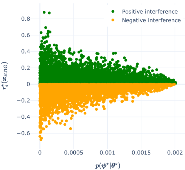
(a) $p(\boldsymbol{\psi}^{\star}|\boldsymbol{\theta}^{\star})$ vs. $r^{\star}(\mathbf{x})$ (linear model).

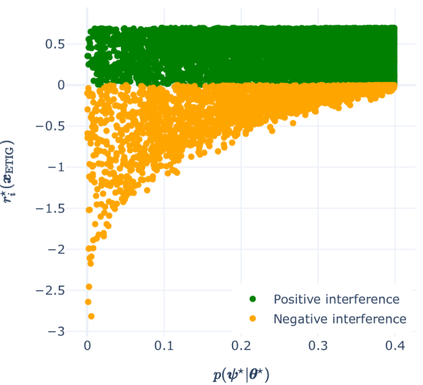
(b) $p(\boldsymbol{\psi}^{\star}|\boldsymbol{\theta}^{\star})$ vs. $r^{\star}(\mathbf{x})$ (preference modeling).

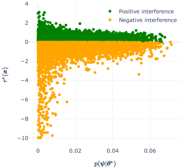
(c) $p(\boldsymbol{\psi}^{\star}|\boldsymbol{\theta}^{\star})$ vs. $r^{\star}(\mathbf{x})$ (GP regression).

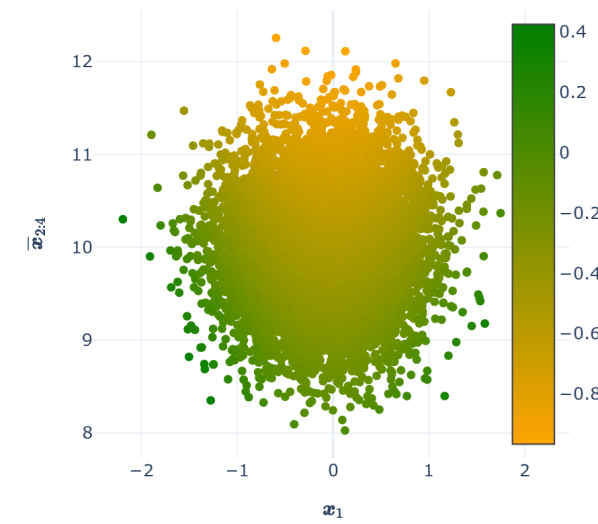
(d) ETIG($\mathbf{x}$) - ELIG($\mathbf{x}$) (linear model).

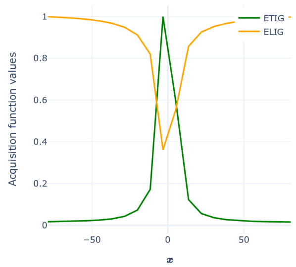
(e) Acquisition function values (preference modeling).

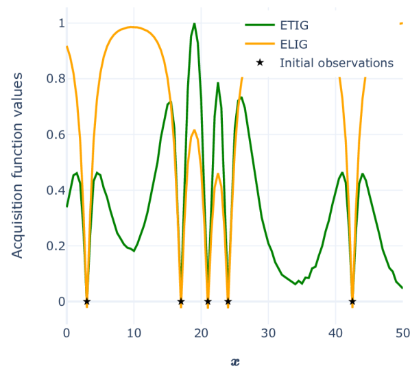
(f) Acquisition function values (GP regression).

Figure 1: Notes. Panels (a–c) show 10,000 parameter values drawn from the learner’s prior. In panel (c), $\mathbf{x}$ is two nearby points in the interior of the domain and values on the $y$-axis are truncated from below at -10. Panels (d–f) show the acquisition function values normalized by their respective maximum values. The acquisition function values in panel (d) are each additionally rescaled so their minima coincide at 0. The $y$-axis in panel (d) is $\frac{\mathbf{x}_{2}+\mathbf{x}_{3}+\mathbf{x}_{4}}{3}$. Panel (f) additionally shows initial training points on which the GP prior used to compute the acquisition function values is conditioned.

The active learner’s dilemma.

Figures 1(d), 1(e) and 1(f) show how the values of the acquisition functions corresponding to the learner’s primary and auxiliary objectives (ETIG and ELIG, respectively) compare to each other. In all cases, there is a trade-off: maximizing with respect to one objective means forgoing gains on the other. For example, Figure 1(d) shows that in the linear model setting, the ETIG is high when the magnitude of $\mathbf{x}_{1}$ is large and the magnitude of $\mathbf{x}_{(2:4)}$ is small; this facilitates identification of the effect of $\mathbf{x}_{1}$. ELIG favors the opposite situation, precisely because it aims for identification of the effects of $\mathbf{x}_{(2:4)}$. Figure 1(f) shows that in the GP regression setting, the ETIG is maximized at points near the training data. Different values of $\boldsymbol{\theta}$ considered by the learner’s prior make different predictions about how correlated these points should be with the training data (while most candidate values $\boldsymbol{\theta}$ predict that points further away will revert to the prior mean). By contrast, ELIG focuses its energies on gaining information about the function as a whole, and so prefers points further away from the training data, where it is most uncertain about the outcomes. See Section B.2 for discussion of the preference modeling setting.

6 CONCLUSION

We analyzed the phenomenon of negative interference, a threat to Bayesian inference posed by the presence of nuisance parameters, and its effect on Bayesian active learning. Our analysis showed that mitigating the threat of negative interference requires the Bayesian active learner to take into account an auxiliary objective: identification of the distribution of nuisance parameters.

A limitation of our analysis is the assumption that the learner has access to the likelihood function. Extensions of our work could apply components of our analysis to the more general setting of potential model misspecification. Our analysis is also limited in the assumption that the partition between target and nuisance parameters is well-defined; in some settings, the learner may additionally be tasked with learning this partition (which can be thought of as a form of relevant feature selection), and/or have the option to eliminate effects of the nuisance parameters (e.g., by controlling laboratory conditions). Finally, an important next step would be to leverage our insights in practice in the form of active learning strategies that incorporate our proposed acquisition function.

Appendix

The appendix is organized as follows:

• In Appendix A, we provide proofs of all our mathematical results.

• In Appendix B, we provide details of the illustrative examples presented in Section 5.

Appendix A PROOFS OF MATHEMATICAL RESULTS

A.1 DEFINITIONS

• $\mathrm{D_{KL}}\left(Q\leavevmode\nobreak\ ||\leavevmode\nobreak\ P\right)$ is the Kullback-Leibler divergence from $Q$ to $P$:

  $$\mathrm{D_{KL}}\left(Q\leavevmode\nobreak\ ||\leavevmode\nobreak\ P\right)=\int_{\mathscr{Y}}\log{\frac{q(\mathbf{y})}{p(\mathbf{y})}}\leavevmode\nobreak\ q(\mathbf{y})\leavevmode\nobreak\ d\mathbf{y}$$

• $\mathrm{H}\left(Q\leavevmode\nobreak\ ||\leavevmode\nobreak\ P\right)$ is the cross-entropy from $Q$ to $P$:

  $$\mathrm{H}\left(Q\leavevmode\nobreak\ ||\leavevmode\nobreak\ P\right)=-\int_{\mathscr{Y}}\log{\left(p(\mathbf{y})\right)}\leavevmode\nobreak\ q(\mathbf{y})\leavevmode\nobreak\ d\mathbf{y}$$

• $\mathrm{H}\left(Q\right)$ is the entropy of distribution $Q$:

  $$\mathrm{H}\left(Q\right)=-\int_{\mathscr{Y}}\log{\left(q(\mathbf{y})\right)}\leavevmode\nobreak\ q(\mathbf{y})\leavevmode\nobreak\ d\mathbf{y}$$

A.2 DERIVATION OF PROPOSITION 4.1

$$r^{\star}{}(\mathbf{x}) =\mathop{\mathbb{E}}_{\mathbf{y}\sim Q_{\mathbf{Y}|\mathbf{x}}}\left[\log{\frac{p(\mathbf{y}|\mathbf{x},\boldsymbol{\theta}^{\star})}{p(\mathbf{y}|\mathbf{x})}}\right]$$

$$=\mathrm{H}\left(Q_{\mathbf{Y}|\mathbf{x}}\leavevmode\nobreak\ ||\leavevmode\nobreak\ P_{\mathbf{Y}|\mathbf{x}}\right)-\mathrm{H}\left(Q_{\mathbf{Y}|\mathbf{x}}\leavevmode\nobreak\ ||\leavevmode\nobreak\ P_{\mathbf{Y}|\mathbf{x},\boldsymbol{\theta}^{\star}}\right)$$

$$=\mathrm{H}\left(Q_{\mathbf{Y}|\mathbf{x}}\right)+\mathrm{D_{KL}}\left(Q_{\mathbf{Y}|\mathbf{x}}\leavevmode\nobreak\ ||\leavevmode\nobreak\ P_{\mathbf{Y}|\mathbf{x}}\right)-\mathrm{H}\left(Q_{\mathbf{Y}|\mathbf{x}}\right)-\mathrm{D_{KL}}\left(Q_{\mathbf{Y}|\mathbf{x}}\leavevmode\nobreak\ ||\leavevmode\nobreak\ P_{\mathbf{Y}|\mathbf{x},\boldsymbol{\theta}^{\star}}\right)$$

$$=\mathrm{D_{KL}}\left(Q_{\mathbf{Y}|\mathbf{x}}\leavevmode\nobreak\ ||\leavevmode\nobreak\ P_{\mathbf{Y}|\mathbf{x}}\right)-\mathrm{D_{KL}}\left(Q_{\mathbf{Y}|\mathbf{x}}\leavevmode\nobreak\ ||\leavevmode\nobreak\ P_{\mathbf{Y}|\mathbf{x},\boldsymbol{\theta}^{\star}}\right)$$

A.3 PROOF OF THEOREM 4.5

The proof of Theorem 4.5 depends on Lemma A.1, which upper bounds $\mathcal{D}$ as a function of $\mathcal{D}_{\boldsymbol{\theta}^{\star}}$.

Lemma A.1 (Upper bound of $\mathcal{D}{}$.).

Given $(\boldsymbol{\theta}^{\star},Q_{\mathbf{\Psi}})$ and $\epsilon$ that satisfies 4.4, $\mathcal{D}$ is upper-bounded as

$$\mathcal{D}{}\leq\left(\int_{N_{\epsilon}(\boldsymbol{\theta}^{\star})}p(\boldsymbol{\theta})\leavevmode\nobreak\ d\boldsymbol{\theta}\right)\mathcal{D}_{\boldsymbol{\theta}^{\star}}+\left(\int_{\mathscr{T}\backslash N_{\epsilon}(\boldsymbol{\theta}^{\star})}p(\boldsymbol{\theta})\leavevmode\nobreak\ d\boldsymbol{\theta}\right)\widetilde{\mathcal{D}}$$

Proof.

$$\mathcal{D}{} =\mathrm{D_{KL}}\left(Q_{\mathbf{Y}|\mathbf{x}}\leavevmode\nobreak\ ||\leavevmode\nobreak\ P_{\mathbf{Y}|\mathbf{x}}\right)$$ (Proposition 4.1)

$$=\int_{\mathscr{Y}}\log{\frac{q(\mathbf{y}|\mathbf{x})}{p(\mathbf{y}|\mathbf{x})}}\leavevmode\nobreak\ q(\mathbf{y}|\mathbf{x})\leavevmode\nobreak\ d\mathbf{y}$$

$$=\int_{\mathscr{Y}}\left(\log{\left(q(\mathbf{y}|\mathbf{x})\right)}-\log{\left(p(\mathbf{y}|\mathbf{x})\right)}\right)\leavevmode\nobreak\ q(\mathbf{y}|\mathbf{x})\leavevmode\nobreak\ d\mathbf{y}$$

$$\leq\int_{\mathscr{Y}}\left(\log{q(\mathbf{y}|\mathbf{x})}-\left(\int_{N_{\epsilon}(\boldsymbol{\theta}^{\star})}p(\boldsymbol{\theta})\leavevmode\nobreak\ d\boldsymbol{\theta}\right)\log{\left(p(\mathbf{y}|\mathbf{x},\boldsymbol{\theta}^{\star})\right)}-\left(\int_{\mathscr{T}\backslash N_{\epsilon}(\boldsymbol{\theta}^{\star})}p(\boldsymbol{\theta})\leavevmode\nobreak\ d\boldsymbol{\theta}\right)\log{\tilde{p}\left(\mathbf{y}|\mathbf{x}\right)}\right)\leavevmode\nobreak\ q(\mathbf{y}|\mathbf{x})\leavevmode\nobreak\ d\mathbf{y}$$

$$\leavevmode\nobreak\ (\text{\lx@cref{creftypecap~refnum}{as:continuity}})$$

$$=-\mathrm{H}\left(Q_{\mathbf{Y}|\mathbf{x}}\right)+\left(\int_{N_{\epsilon}(\boldsymbol{\theta}^{\star})}p(\boldsymbol{\theta})\leavevmode\nobreak\ d\boldsymbol{\theta}\right)\mathrm{H}\left(Q_{\mathbf{Y}|\mathbf{x}}\leavevmode\nobreak\ ||\leavevmode\nobreak\ P_{\mathbf{Y}|\mathbf{x},\boldsymbol{\theta}^{\star}}\right)+\left(\int_{\mathscr{T}\backslash N_{\epsilon}(\boldsymbol{\theta}^{\star})}p(\boldsymbol{\theta})\leavevmode\nobreak\ d\boldsymbol{\theta}\right)\mathrm{H}\left(Q_{\mathbf{Y}|\mathbf{x}}\leavevmode\nobreak\ ||\leavevmode\nobreak\ \tilde{P}_{\mathbf{Y}|\mathbf{x}}\right)$$

$$=-\mathrm{H}\left(Q_{\mathbf{Y}|\mathbf{x}}\right)+\left(\int_{N_{\epsilon}(\boldsymbol{\theta}^{\star})}p(\boldsymbol{\theta})\leavevmode\nobreak\ d\boldsymbol{\theta}\right)\left(\mathrm{H}\left(Q_{\mathbf{Y}|\mathbf{x}}\right)+\mathrm{D_{KL}}\left(Q_{\mathbf{Y}|\mathbf{x}}\leavevmode\nobreak\ ||\leavevmode\nobreak\ P_{\mathbf{Y}|\mathbf{x},\boldsymbol{\theta}^{\star}}\right)\right)$$

$$\leavevmode\nobreak\ \leavevmode\nobreak\ \leavevmode\nobreak\ \leavevmode\nobreak\ \leavevmode\nobreak\ +\left(\int_{\mathscr{T}\backslash N_{\epsilon}(\boldsymbol{\theta}^{\star})}p(\boldsymbol{\theta})\leavevmode\nobreak\ d\boldsymbol{\theta}\right)\left(\mathrm{H}\left(Q_{\mathbf{Y}|\mathbf{x}}\right)+\mathrm{D_{KL}}\left(Q_{\mathbf{Y}|\mathbf{x}}\leavevmode\nobreak\ ||\leavevmode\nobreak\ \tilde{P}_{\mathbf{Y}|\mathbf{x}}\right)\right)$$

$$=\left(\int_{N_{\epsilon}(\boldsymbol{\theta}^{\star})}p(\boldsymbol{\theta})\leavevmode\nobreak\ d\boldsymbol{\theta}\right)\mathrm{D_{KL}}\left(Q_{\mathbf{Y}|\mathbf{x}}\leavevmode\nobreak\ ||\leavevmode\nobreak\ P_{\mathbf{Y}|\mathbf{x},\boldsymbol{\theta}^{\star}}\right)+\left(\int_{\mathscr{T}\backslash N_{\epsilon}(\boldsymbol{\theta}^{\star})}p(\boldsymbol{\theta})\leavevmode\nobreak\ d\boldsymbol{\theta}\right)\mathrm{D_{KL}}\left(Q_{\mathbf{Y}|\mathbf{x}}\leavevmode\nobreak\ ||\leavevmode\nobreak\ \tilde{P}_{\mathbf{Y}|\mathbf{x}}\right)$$

$$=\left(\int_{N_{\epsilon}(\boldsymbol{\theta}^{\star})}p(\boldsymbol{\theta})\leavevmode\nobreak\ d\boldsymbol{\theta}\right)\mathcal{D}_{\boldsymbol{\theta}^{\star}}+\left(\int_{\mathscr{T}\backslash N_{\epsilon}(\boldsymbol{\theta}^{\star})}p(\boldsymbol{\theta})\leavevmode\nobreak\ d\boldsymbol{\theta}\right)\widetilde{\mathcal{D}}$$

∎

Direct substitution of this bound into Proposition 4.1 completes the proof of Theorem 4.5:

$$r^{\star}(\mathbf{x}) =\mathcal{D}+\mathcal{D}_{\boldsymbol{\theta}^{\star}}$$ (Proposition 4.1)

$$\leq\left(\int_{N_{\epsilon}(\boldsymbol{\theta}^{\star})}p(\boldsymbol{\theta})\leavevmode\nobreak\ d\boldsymbol{\theta}\right)\mathcal{D}_{\boldsymbol{\theta}^{\star}}+\left(\int_{\mathscr{T}\backslash N_{\epsilon}(\boldsymbol{\theta}^{\star})}p(\boldsymbol{\theta})\leavevmode\nobreak\ d\boldsymbol{\theta}\right)\widetilde{\mathcal{D}}-\mathcal{D}_{\boldsymbol{\theta}^{\star}}$$ (Lemma A.1)

$$=\left(\int_{\mathscr{T}\backslash N_{\epsilon}(\boldsymbol{\theta}^{\star})}p(\boldsymbol{\theta})\leavevmode\nobreak\ d\boldsymbol{\theta}\right)\left(\widetilde{\mathcal{D}}-\mathcal{D}_{\boldsymbol{\theta}^{\star}}\right)$$

A.4 PROOF OF THEOREM 4.8

The conditions of Theorem 4.8 imply that $r^{\star}(\mathbf{x})$ can grow arbitrarily negative as $\boldsymbol{\phi}_{i}\rightarrow\infty$ or as $\boldsymbol{\phi}_{i}\rightarrow-\infty$.

If 4.7(a) holds, the conditions of Theorem 4.8 imply that at some point $\tilde{\boldsymbol{\phi}}_{i}$ on dimension $i$ of $\mathscr{F}$, any movement along this dimension towards $-\infty$ will result in $r^{\star}(\mathbf{x})$ decreasing by at least some amount $d$. 4.7(a) implies that $\boldsymbol{\phi}_{i}\rightarrow-\infty$, and the stated conditions imply that $r^{\star}(\mathbf{x})$ can grow arbitrarily negative as $\boldsymbol{\phi}_{i}\rightarrow-\infty$.

More specifically, we require that, for some $\tilde{\boldsymbol{\phi}}$, the following holds $\forall\boldsymbol{\phi}\in\mathscr{F}$ for which $\boldsymbol{\phi}_{i}<\tilde{\boldsymbol{\phi}}_{i}$:

$$\nabla r^{\star}(\mathbf{x})_{i}>d \iff\nabla\mathcal{D}(\mathbf{x})_{i}-\nabla\mathcal{D}_{\boldsymbol{\theta}^{\star}}(\mathbf{x})_{i}>d$$

$$\iff\nabla\mathcal{D}_{\boldsymbol{\theta}^{\star}}(\mathbf{x})_{i}<\nabla\mathcal{D}(\mathbf{x})_{i}-d$$

as stated in the theorem.

If 4.7(b) holds, the conditions of Theorem 4.8 imply that at some point $\tilde{\boldsymbol{\phi}}_{i}$ on dimension $i$ of $\mathscr{F}$, any movement along this dimension towards $\infty$ will result in $r^{\star}(\mathbf{x})$ decreasing by at least some amount $d$. 4.7(b) implies that $\boldsymbol{\phi}_{i}\rightarrow\infty$, and the stated conditions imply that $r^{\star}(\mathbf{x})$ can grow arbitrarily negative as $\boldsymbol{\phi}_{i}\rightarrow\infty$.

For this, we require that, for some $\tilde{\boldsymbol{\phi}}$, the following holds $\forall\boldsymbol{\phi}\in\mathscr{F}$ for which $\boldsymbol{\phi}_{i}>\tilde{\boldsymbol{\phi}}_{i}$:

$$\nabla r^{\star}(\mathbf{x})_{i}<-d \iff\nabla\mathcal{D}(\mathbf{x})_{i}-\nabla\mathcal{D}_{\boldsymbol{\theta}^{\star}}(\mathbf{x})_{i}<-d$$

$$\iff\nabla\mathcal{D}_{\boldsymbol{\theta}^{\star}}(\mathbf{x})_{i}>\nabla\mathcal{D}(\mathbf{x})_{i}+d$$

as stated in the theorem.

Application to the linear model.

We use $\sigma^{2}_{\mathbf{y}|\mathbf{x}}\coloneqq\sigma^{2}+\mathbf{x}\mathbf{\Sigma}\mathbf{x}^{T}$ and $\sigma^{2}_{\mathbf{y}|\mathbf{x},\boldsymbol{\theta}^{\star}}\coloneqq\sigma^{2}+\mathbf{x}\left(\mathbf{\Sigma}_{2,2}-\mathbf{\Sigma}_{1,2}\mathbf{\Sigma}_{1,1}^{-1}\mathbf{\Sigma}_{1,2}\right)\mathbf{x}^{T}$ to refer to the variance of the learner’s predictive distribution and variance of distribution corresponding to the learner’s target likelihood, respectively. Without loss of generality, take $\boldsymbol{\mu}=[0,0]$ and $\mathbf{\Sigma}$ to be a diagonal matrix, and so $\mathop{\mathbb{E}}_{\boldsymbol{\theta}\sim P_{\mathbf{\Theta}}}\left[\boldsymbol{\theta}\right]=0$ and $\mathop{\mathbb{E}}_{\boldsymbol{\psi}\sim P_{\mathbf{\Psi}|\boldsymbol{\theta}^{\star}}}\left[\boldsymbol{\psi}\right]=\mathop{\mathbb{E}}_{\boldsymbol{\psi}\sim P_{\mathbf{\Psi}}}\left[\boldsymbol{\psi}\right]=0$.

As described in the main text, $\boldsymbol{\phi}$ represents the mean of $Q_{\mathbf{\Psi}}$, i.e., $\boldsymbol{\phi}\in\mathbb{R}\coloneqq\mathop{\mathbb{E}}_{\boldsymbol{\psi}\sim Q_{\mathbf{\Psi}}}\left[\boldsymbol{\psi}\right]$. This satisfies 4.7 (for $i=1$). Satisfying the conditions of the theorem requires showing that the conditions on the gradients $\nabla\mathcal{D}_{\boldsymbol{\theta}^{\star}}$ and $\nabla\mathcal{D}$ are met. Below, we give the derivatives $\frac{\partial\mathcal{D}_{\boldsymbol{\theta}^{\star}}}{\partial\boldsymbol{\phi}}$ and $\frac{\partial\mathcal{D}}{\partial\boldsymbol{\phi}}$, and then show that there is a value $\tilde{\boldsymbol{\phi}}$ below which the gradient conditions in 4.7(a) hold, and a value $\tilde{\boldsymbol{\phi}}$ above which the gradient conditions in 4.7(b) hold.

$$\mathcal{D}_{\boldsymbol{\theta}^{\star}} =\mathrm{D_{KL}}\left(Q_{\mathbf{Y}|\mathbf{x}}\leavevmode\nobreak\ ||\leavevmode\nobreak\ P_{\mathbf{Y}|\mathbf{x},\boldsymbol{\theta}^{\star}}\right)$$

$$=\frac{1}{2}\left(\left(\frac{\sigma^{2}}{\sigma^{2}_{\mathbf{y}|\mathbf{x},\boldsymbol{\theta}^{\star}}}\right)+\frac{\left(\boldsymbol{\theta}^{\star}x_{1}+\mathop{\mathbb{E}}_{\boldsymbol{\psi}\sim P_{\mathbf{\Psi}|\boldsymbol{\theta}^{\star}}}\left[\boldsymbol{\psi}x_{2}\right]-\left(\boldsymbol{\theta}^{\star}x_{1}+\mathop{\mathbb{E}}_{\boldsymbol{\psi}\sim Q_{\mathbf{\Psi}}}\left[\boldsymbol{\psi}x_{2}\right]\right)\right)^{2}}{\sigma^{2}_{\mathbf{y}|\mathbf{x},\boldsymbol{\theta}^{\star}}}-1+\log{\frac{\sigma^{2}_{\mathbf{y}|\mathbf{x},\boldsymbol{\theta}^{\star}}}{\sigma^{2}}}\right)$$

$$=\frac{1}{2}\left(\left(\frac{\sigma^{2}}{\sigma^{2}_{\mathbf{y}|\mathbf{x},\boldsymbol{\theta}^{\star}}}\right)+\frac{\left(-\boldsymbol{\phi}x_{2}\right)^{2}}{\sigma^{2}_{\mathbf{y}|\mathbf{x},\boldsymbol{\theta}^{\star}}}-1+\log{\frac{\sigma^{2}_{\mathbf{y}|\mathbf{x},\boldsymbol{\theta}^{\star}}}{\sigma^{2}}}\right)$$

$$\frac{\partial\mathcal{D}_{\boldsymbol{\theta}^{\star}}}{\partial\boldsymbol{\phi}} =\frac{\boldsymbol{\phi}x_{2}^{2}}{\sigma^{2}_{\mathbf{y}|\mathbf{x},\boldsymbol{\theta}^{\star}}}$$

$$\mathcal{D} =\mathrm{D_{KL}}\left(Q_{\mathbf{Y}|\mathbf{x}}\leavevmode\nobreak\ ||\leavevmode\nobreak\ P_{\mathbf{Y}|\mathbf{x}}\right)$$

$$=\frac{1}{2}\left(\left(\frac{\sigma^{2}}{\sigma^{2}_{\mathbf{y}|\mathbf{x}}}\right)+\frac{\left(\mathop{\mathbb{E}}_{\boldsymbol{\theta},\boldsymbol{\psi}\sim P_{\mathbf{\Theta},\mathbf{\Psi}}}\left[\boldsymbol{\theta}x_{1}+\boldsymbol{\psi}x_{2}\right]-\left(\boldsymbol{\theta}^{\star}x_{1}+\mathop{\mathbb{E}}_{\boldsymbol{\psi}\sim Q_{\mathbf{\Psi}}}\left[\boldsymbol{\psi}x_{2}\right]\right)\right)^{2}}{\sigma^{2}_{\mathbf{y}|\mathbf{x}}}-1+\log{\frac{\sigma^{2}_{\mathbf{y}|\mathbf{x}}}{\sigma^{2}}}\right)$$

$$=\frac{1}{2}\left(\left(\frac{\sigma^{2}}{\sigma^{2}_{\mathbf{y}|\mathbf{x}}}\right)+\frac{\left(\boldsymbol{\theta}^{\star}x_{1}+\boldsymbol{\phi}x_{2}\right)^{2}}{\sigma^{2}_{\mathbf{y}|\mathbf{x}}}-1+\log{\frac{\sigma^{2}_{\mathbf{y}|\mathbf{x}}}{\sigma^{2}}}\right)$$

$$\frac{\partial\mathcal{D}}{\partial\boldsymbol{\phi}} =\frac{\boldsymbol{\theta}^{\star}x_{1}x_{2}+\boldsymbol{\phi}x_{2}^{2}}{\sigma^{2}_{\mathbf{y}|\mathbf{x}}}$$

$$\frac{\partial\mathcal{D}_{\boldsymbol{\theta}^{\star}}}{\partial\boldsymbol{\phi}}-\frac{\partial\mathcal{D}}{\partial\boldsymbol{\phi}} =\frac{\boldsymbol{\phi}x_{2}^{2}}{\sigma^{2}_{\mathbf{y}|\mathbf{x},\boldsymbol{\theta}^{\star}}}-\frac{\boldsymbol{\theta}^{\star}x_{1}x_{2}+\boldsymbol{\phi}x_{2}^{2}}{\sigma^{2}_{\mathbf{y}|\mathbf{x}}}$$

$$=\boldsymbol{\phi}\left(\frac{x_{2}^{2}}{\sigma^{2}_{\mathbf{y}|\mathbf{x},\boldsymbol{\theta}^{\star}}}-\frac{x_{2}^{2}}{\sigma^{2}_{\mathbf{y}|\mathbf{x}}}\right)-\frac{\boldsymbol{\theta}^{\star}x_{1}x_{2}}{\sigma^{2}_{\mathbf{y}|\mathbf{x}}}$$ (2)

Taking $\rho=\frac{x_{2}^{2}}{\sigma^{2}_{\mathbf{y}|\mathbf{x},\boldsymbol{\theta}^{\star}}}-\frac{x_{2}^{2}}{\sigma^{2}_{\mathbf{y}|\mathbf{x}}}\geq 0$ (since $\sigma^{2}_{\mathbf{y}|\mathbf{x},\boldsymbol{\theta}^{\star}}$ can never be greater than $\sigma^{2}_{\mathbf{y}|\mathbf{x}}$) and $\tau=\frac{\boldsymbol{\theta}^{\star}x_{1}x_{2}}{\sigma^{2}_{\mathbf{y}|\mathbf{x}}}$, Equation 2 is at most $-d$ when $\boldsymbol{\phi}\leq\frac{\tau-d}{\rho}$, and so the conditions in Theorem 4.8(a) are met for any $\tilde{\phi}\leq\frac{\tau-d}{\rho}$.

Equation 2 is at least $d$ when $\boldsymbol{\phi}\geq\frac{\tau+d}{\rho}$, and so the conditions in Theorem 4.8(b) are met for any $\tilde{\phi}\geq\frac{\tau+d}{\rho}$.

A.5 PROOF OF THEOREM 4.11

We first given the proof of Lemma 4.10.

Proof.

Take $p^{\alpha}(\mathbf{y}|\mathbf{x},\boldsymbol{\theta}^{\star})$ to be the likelihood of $\mathbf{y}$ under the $Q_{\mathbf{\Psi}}$-mixed prior $P_{\mathbf{\Psi}|\boldsymbol{\theta}^{\star}}^{\alpha}$.

$$\mathcal{D}_{\boldsymbol{\theta}^{\star}}(\alpha) =\mathrm{D_{KL}}\left(Q_{\mathbf{Y}|\mathbf{x}}\leavevmode\nobreak\ ||\leavevmode\nobreak\ P_{\mathbf{Y}|\mathbf{x},\boldsymbol{\theta}^{\star}}^{\alpha}\right)$$

$$=\int_{\mathscr{Y}}\log{\frac{q(\mathbf{y}|\mathbf{x})}{p^{\alpha}(\mathbf{y}|\mathbf{x},\boldsymbol{\theta}^{\star})}}\leavevmode\nobreak\ q(\mathbf{y}|\mathbf{x})\leavevmode\nobreak\ d\mathbf{y}$$

$$=\int_{\mathscr{Y}}\log{\frac{\mathop{\mathbb{E}}_{\boldsymbol{\psi}\sim Q_{\mathbf{\Psi}}}\left[p(\mathbf{y}|\mathbf{x},\boldsymbol{\theta}^{\star},\boldsymbol{\psi})\right]}{\mathop{\mathbb{E}}_{\boldsymbol{\psi}\sim P_{\mathbf{\Psi}|\boldsymbol{\theta}^{\star}}^{\alpha}}\left[p(\mathbf{y}|\mathbf{x},\boldsymbol{\theta}^{\star},\boldsymbol{\psi})\right]}}\leavevmode\nobreak\ q(\mathbf{y}|\mathbf{x})\leavevmode\nobreak\ d\mathbf{y}$$

$$=\int_{\mathscr{Y}}\log{\frac{\mathop{\mathbb{E}}_{\boldsymbol{\psi}\sim Q_{\mathbf{\Psi}}}\left[p(\mathbf{y}|\mathbf{x},\boldsymbol{\theta}^{\star},\boldsymbol{\psi})\right]}{\alpha\mathop{\mathbb{E}}_{\boldsymbol{\psi}\sim Q_{\mathbf{\Psi}}}\left[p(\mathbf{y}|\mathbf{x},\boldsymbol{\theta}^{\star},\boldsymbol{\psi})\right]+(1-\alpha)\mathop{\mathbb{E}}_{\boldsymbol{\psi}\sim P_{\mathbf{\Psi}|\boldsymbol{\theta}^{\star}}}\left[p(\mathbf{y}|\mathbf{x},\boldsymbol{\theta}^{\star},\boldsymbol{\psi})\right]}}\leavevmode\nobreak\ q(\mathbf{y}|\mathbf{x})\leavevmode\nobreak\ d\mathbf{y}$$

$$=-\int_{\mathscr{Y}}\log{\left(\alpha+\left(1-\alpha\right)\frac{\mathop{\mathbb{E}}_{\boldsymbol{\psi}\sim P_{\mathbf{\Psi}|\boldsymbol{\theta}^{\star}}}\left[p(\mathbf{y}|\mathbf{x},\boldsymbol{\theta}^{\star},\boldsymbol{\psi})\right]}{\mathop{\mathbb{E}}_{\boldsymbol{\psi}\sim Q_{\mathbf{\Psi}}}\left[p(\mathbf{y}|\mathbf{x},\boldsymbol{\theta}^{\star},\boldsymbol{\psi})\right]}\right)}\leavevmode\nobreak\ q(\mathbf{y}|\mathbf{x})\leavevmode\nobreak\ d\mathbf{y}$$

$$=-\int_{\mathscr{Y}}\log{\left(\alpha+\left(1-\alpha\right)\frac{p(\mathbf{y}|\mathbf{x},\boldsymbol{\theta}^{\star})}{q(\mathbf{y}|\mathbf{x})}\right)}\leavevmode\nobreak\ q(\mathbf{y}|\mathbf{x})\leavevmode\nobreak\ d\mathbf{y}$$

$$\geq-\log{\left(\int_{\mathscr{Y}}\left(\alpha+\left(1-\alpha\right)\frac{p(\mathbf{y}|\mathbf{x},\boldsymbol{\theta}^{\star})}{q(\mathbf{y}|\mathbf{x})}\right)\leavevmode\nobreak\ q(\mathbf{y}|\mathbf{x})\leavevmode\nobreak\ d\mathbf{y}\right)}$$ (Jensen’s inequality)

$$=-\log{\left(\alpha+\left(1-\alpha\right)\left(\int_{\mathscr{Y}}\frac{p(\mathbf{y}|\mathbf{x},\boldsymbol{\theta}^{\star})}{q(\mathbf{y}|\mathbf{x})}\leavevmode\nobreak\ q(\mathbf{y}|\mathbf{x})\leavevmode\nobreak\ d\mathbf{y}\right)\right)}$$ (3)

∎

For the proof of Theorem 4.8, we can without loss of generality take $\alpha_{1}=0$ and $\alpha_{2}\in(0,1]$. (Notice that for any $P_{\mathbf{\Psi}|\boldsymbol{\theta}^{\star}}$ and $\alpha_{1}>0$ we could take the prior $P_{\mathbf{\Psi}|\boldsymbol{\theta}^{\star}}^{\alpha_{1}}=\alpha_{1}Q_{\mathbf{\Psi}}+(1-\alpha_{1})P_{\mathbf{\Psi}|\boldsymbol{\theta}^{\star}}$ $Q_{\mathbf{\Psi}}$-mixed at rate 0, which would be equivalent to $P_{\mathbf{\Psi}|\boldsymbol{\theta}^{\star}}$ $Q_{\mathbf{\Psi}}$-mixed at rate $\alpha_{1}$.) When $\alpha=0$, we can use the usual notation for the prior and bias terms.

By Proposition 4.1, we can say that if $P_{\mathbf{\Psi}|\mathbf{x}}$ induces negative interference under the given DGP:

$$\mathcal{D}_{\boldsymbol{\theta}^{\star}} >\mathcal{D}$$

$$-\mathcal{D}_{\boldsymbol{\theta}^{\star}} <-\mathcal{D}$$

$$-\int_{\mathscr{Y}}\log{\frac{q(\mathbf{y}|\mathbf{x})}{p(\mathbf{y}|\mathbf{x},\boldsymbol{\theta}^{\star})}}\leavevmode\nobreak\ q(\mathbf{y}|\mathbf{x})\leavevmode\nobreak\ d\mathbf{y} <-\mathcal{D}$$

$$-\log{\int_{\mathscr{Y}}\frac{q(\mathbf{y}|\mathbf{x})}{p(\mathbf{y}|\mathbf{x},\boldsymbol{\theta}^{\star})}\leavevmode\nobreak\ q(\mathbf{y}|\mathbf{x})\leavevmode\nobreak\ d\mathbf{y}} <-\mathcal{D}$$ (Jensen’s inequality)

$$\log{\int_{\mathscr{Y}}\frac{p(\mathbf{y}|\mathbf{x},\boldsymbol{\theta}^{\star})}{q(\mathbf{y}|\mathbf{x})}\leavevmode\nobreak\ q(\mathbf{y}|\mathbf{x})\leavevmode\nobreak\ d\mathbf{y}} <-\mathcal{D}$$

$$\int_{\mathscr{Y}}\frac{p(\mathbf{y}|\mathbf{x},\boldsymbol{\theta}^{\star})}{q(\mathbf{y}|\mathbf{x})}\leavevmode\nobreak\ q(\mathbf{y}|\mathbf{x})\leavevmode\nobreak\ d\mathbf{y} <e^{-\mathcal{D}}$$

$$<1$$

The last line follows since $e^{-\mathcal{D}}\geq 1$ would violate the non-negativity of the Kullback-Leibler divergence measure that defines $\mathcal{D}$.

Since $\int_{\mathscr{Y}}\frac{p(\mathbf{y}|\mathbf{x},\boldsymbol{\theta}^{\star})}{q(\mathbf{y}|\mathbf{x})}\leavevmode\nobreak\ q(\mathbf{y}|\mathbf{x})\leavevmode\nobreak\ d\mathbf{y}<1$, we can say that if $P_{\mathbf{\Psi}|\mathbf{x}}$ induces negative interference under the given DGP, the expression in line 3 generally decreases with $\alpha$. Comparison between $\alpha=0$ and $\alpha\in(0,1]$ recovers the statement in the theorem for $\alpha_{1}=0$, which can be generalized to all $\alpha_{1}\in[0,1)$ and $\alpha_{2}\in(0,1]>\alpha_{1}$ as described above.

Appendix B DETAILS OF ILLUSTRATIVE EXAMPLES

B.1 LINEAR MODEL

Data was generated according to the model $\mathbf{y}\sim\mathcal{N}\left(\boldsymbol{\theta}\mathbf{x}_{1}+\boldsymbol{\psi}_{1}\mathbf{x}_{2}+\boldsymbol{\psi}_{2}\mathbf{x}_{3}+\boldsymbol{\psi}_{3}\mathbf{x}_{4},\sigma^{2}\right)$ where $\sigma^{2}=1$. The learner’s prior over $\left(\mathbf{\Theta},\mathbf{\Psi}_{1},\mathbf{\Psi}_{2},\mathbf{\Psi}_{3}\right)$ is $\mathcal{N}\left(M,S\right)$ where $M=\begin{bmatrix}0&0&0&0\end{bmatrix}$ and $S=\begin{bmatrix}10&0&0&0\\ 0&10&0&0\\ 0&0&10&0\\ 0&0&0&10\end{bmatrix}$. We used the following formulas to calculate the ETIG and ELIG:

$$\mathrm{ETIG}(\mathbf{x}) =\frac{1}{2}\log{\left(\frac{\sigma^{2}+\mathbf{x}S\mathbf{x}^{T}}{\sigma^{2}+\mathbf{x}\left(S_{(2:4),(2:4)}-S_{1,(2:4)}S_{1}^{-1}S_{1,(2:4)}\right)\mathbf{x}^{T}}\right)}$$

$$\mathrm{ELIG}(\mathbf{x}) =\frac{1}{2}\left(\log{\left(\frac{\sigma^{2}+\mathbf{x}S\mathbf{x}^{T}}{\sigma^{2}}\right)}-\log{\left(\frac{\sigma^{2}+\mathbf{x}S\mathbf{x}^{T}}{\sigma^{2}+\mathbf{x}\left(S_{(2:4),(2:4)}-S_{1,(2:4)}S_{1}^{-1}S_{1,(2:4)}\right)\mathbf{x}^{T}}\right)}\right)$$

To generate the set of possible actions, we sampled 10,000 values $\boldsymbol{z}\sim\mathcal{N}(10,.25)$. For each value $\boldsymbol{z}$, we then sampled one value of each $\mathbf{x}_{2}$, $\mathbf{x}_{3}$ and $\mathbf{x}_{4}$ from $\mathcal{N}(\boldsymbol{z},.25)$, and one value $\mathbf{x}_{1}$ from $\mathcal{N}(-1/\boldsymbol{z},.25)$. Each point in Figure 1(d) corresponds to one of 10,000 values of $\mathscr{\mathbf{x}}$ generated as above. With reference to Figure 1(a), when we calculate $r^{\star}(\mathbf{x})$, $\mathbf{x}$ is always $\mathop{\mathrm{argmax}}_{\mathbf{x}\in\mathscr{X}}\mathrm{ETIG(\mathbf{x})}$ where $\mathscr{X}$ contains all 10,000 possible actions.

B.2 PREFERENCE MODELING

We modified the preference example from Foster et al., (2019), who use a censored sigmoid normal as the output distribution. Instead, we used the Bernoulli distribution $\mathbf{y}\sim\mathrm{Bernoulli}\left(\frac{1}{1+e^{\boldsymbol{\psi}\mathbf{x}-\boldsymbol{\theta}}}\right)$. In our example, the learner’s prior over $\left(\mathbf{\Theta},\mathbf{\Psi}\right)$ was $\mathcal{N}\left(\begin{bmatrix}0&0\end{bmatrix},\begin{bmatrix}16&0\\ 0&1\end{bmatrix}\right)$.

Figure 1(b) shows the $r^{\star}(\mathbf{x})$ for $\mathbf{x}=\mathop{\mathrm{argmax}}_{\mathbf{x}\in\mathscr{X}}\mathrm{ETIG(\mathbf{x})}$ where $\mathscr{X}$ contains values evenly spaced between -79 and 81 (this differs slightly from the example in Foster et al., (2019), in which values of $\mathbf{x}$ were evenly spaced between -80 and 80).

Unlike in the linear model setting, for which there are closed-form expressions for the ETIG and ELIG, the ETIG and ELIG for this example are not known in closed form. We approximate them using the following nested Monte Carlo estimators:

$$\widehat{\text{ETIG}}(\mathbf{x})=\sum_{i=1}^{N}\left(\sum_{\mathbf{y}\in\mathscr{Y}}\left(p(\mathbf{y}|\mathbf{x},\boldsymbol{\theta}^{i},\boldsymbol{\psi}^{i})\log{\frac{\sum_{j=1}^{M}p(\mathbf{y}|\mathbf{x},\boldsymbol{\theta}^{i},\boldsymbol{\psi}^{j})}{\sum_{l=1}^{N}p(\mathbf{y}|\mathbf{x},\boldsymbol{\theta}^{l},\boldsymbol{\psi}^{l})}}\right)\right)$$ (4)

$$\widehat{\text{ELIG}}(\mathbf{x}) =\sum_{i=1}^{N}\left(\sum_{\mathbf{y}\in\mathscr{Y}}\left(p(\mathbf{y}|\mathbf{x},\boldsymbol{\theta}^{i},\boldsymbol{\psi}^{i})\log{\frac{p(\mathbf{y}|\mathbf{x},\boldsymbol{\theta}^{i},\boldsymbol{\psi}^{i})}{\sum_{l=1}^{N}p(\mathbf{y}|\mathbf{x},\boldsymbol{\theta}^{l},\boldsymbol{\psi}^{l})}}\right)\right)-\widehat{\text{ETIG}}(\mathbf{x})$$ (5)

Samples of $\boldsymbol{\theta}$ and $\boldsymbol{\psi}$ are drawn from the prior given above. Although not shown explicitly in Equation 4, each set of $M$ inner samples is constrained to include the corresponding sample $\left(\boldsymbol{\theta}^{i},\boldsymbol{\psi}^{i}\right)$ to avoid pathological behavior when a value $\mathbf{y}$ has positive probability in only a very small region of $P_{\mathbf{\Psi}|\boldsymbol{\theta}^{i}}$ (Foster et al.,, 2020). We set $N$ to 10,000 and $M$ to 100 (reflecting results from Rainforth et al., (2018) that $M$ is optimally $\propto\sqrt{N}$).

Remark on Figure 1(e). The trade-off between ETIG and ELIG visualized in Figure 1(e) can be explained by noticing that the magnitude of $\mathbf{x}$ has opposite effects on the ease of identification of $\boldsymbol{\theta}$ and $\boldsymbol{\psi}$. When $\mathbf{x}=0$, $\boldsymbol{\psi}\mathbf{x}=0$ and so $\boldsymbol{\psi}$ can’t be identified at all. This is reflected by the fact that the ETIG peaks at 0. Conversely, the size of the effect of $\boldsymbol{\psi}$ on outcomes depends on the magnitude of $\mathbf{x}$, which is reflected by the fact that the ELIG is maximized by values of $\mathbf{x}$ with large magnitudes.

B.3 GAUSSIAN PROCESS REGRESSION

We constructed the kernel $k(\cdot,\cdot)$ as the additive composition of $k_{\boldsymbol{\theta}}(\cdot,\cdot)$ and $k_{\boldsymbol{\psi}_{1}}(\cdot,\cdot)$ where both $k_{\boldsymbol{\theta}}(\cdot,\cdot)$ and $k_{\boldsymbol{\psi}_{1}}(\cdot,\cdot)$ were radial basis functions kernels with shared amplitude and lengthscale determined by the values $\boldsymbol{\theta}$ and $\boldsymbol{\psi}_{1}$, respectively. Both $P_{\mathbf{\Theta}}$ and $P_{\mathbf{\Psi}_{1}}$ were Gamma distributions with concentration 3 and scale 1.25.

To generate Figure 1(c), we set $\mathbf{x}=[25,26]$, and sampled 10,000 values from the learner’s joint distribution over $(\boldsymbol{\theta},\boldsymbol{\psi}_{1},\boldsymbol{\psi}_{2})$, where $\boldsymbol{\psi}_{2}$ is a sample from the GP at $\mathbf{x}$. We set $\sigma^{2}$, the variance of $\mathbf{Y}|\mathbf{x},\boldsymbol{\theta},\boldsymbol{\psi}_{1},\boldsymbol{\psi}_{2}$, to .01.

We approximated $r^{\star}(\mathbf{x})$ using a nested Monte Carlo estimator:

$$r^{\star}(\mathbf{x}) =\mathop{\mathbb{E}}_{\mathbf{y}\sim P_{\mathbf{Y}|\boldsymbol{\theta}^{\star},\boldsymbol{\psi}^{\star}}}\left[\log{(p(\mathbf{y}|\mathbf{x},\boldsymbol{\theta}^{\star})}-\log{(p(\mathbf{y}|\mathbf{x})}\right]$$

$$\approx\frac{1}{M}\sum_{i=1}^{M}\left(\log{\left(\frac{1}{M}\sum_{j=1}^{M}p(y^{i}|\mathbf{x},\boldsymbol{\theta}^{\star},\boldsymbol{\psi}^{j})\right)}-\log{\left(\frac{1}{N}\sum_{j=1}^{N}p(y^{i}|\mathbf{x},\boldsymbol{\theta}^{j},\boldsymbol{\psi}^{j})\right)}\right)$$

with $N=10,000$ and $M=100$. Samples were drawn from the prior given above.

To generate Figure 1(f), we used a Hamiltonian Monte Carlo (HMC) sampler (Gardner et al.,, 2018) to first train the model, initialized with the priors given above, on the five randomly-sampled points shown in the figure. The training data was generated from a function sampled from a kernel with $\boldsymbol{\theta}^{\star}=5$ and $\boldsymbol{\psi}_{1}^{\star}=2.5$. In this case, $\sigma^{2}=0$, i.e., outcomes were treated as deterministic. We again used nested Monte Carlo estimators for the acquisition functions, given below. Rather than sampling from the prior, we used the HMC samples of $\boldsymbol{\theta}$ and $\boldsymbol{\psi}_{1}$ to compute the expectations.

$$\mathrm{ETIG}(\mathbf{x}) =\mathop{\mathbb{E}}_{\boldsymbol{\theta},\boldsymbol{\psi},\mathbf{y}\sim P_{\mathbf{\Theta},\mathbf{\Psi},\mathbf{Y}|\mathbf{x}}}\left[\log{(p(\mathbf{y}|\mathbf{x},\boldsymbol{\theta})}-\log{(p(\mathbf{y}|\mathbf{x})}\right]$$

$$\approx\frac{1}{N}\sum_{i=1}^{N}\left(\frac{1}{L}\sum_{l=1}^{L}\log{\left(\frac{1}{M}\sum_{j=1}^{M}p(\mathbf{y}^{l}|\mathbf{x},\boldsymbol{\theta}^{i},\boldsymbol{\psi}^{j})\right)}-\frac{1}{L}\sum_{l=1}^{L}\log{\left(\frac{1}{N}\sum_{j=1}^{N}p(\mathbf{y}^{l}|\mathbf{x},\boldsymbol{\theta}^{j},\boldsymbol{\psi}^{j})\right)}\right)$$

$$\mathrm{ELIG}(\mathbf{x}) =\mathop{\mathbb{E}}_{\boldsymbol{\theta},\boldsymbol{\psi},\mathbf{y}\sim P_{\mathbf{\Theta},\mathbf{\Psi},\mathbf{Y}|\mathbf{x}}}\left[\log{(p(\mathbf{y}|\mathbf{x},\boldsymbol{\theta},\boldsymbol{\psi})}-\log{(p(\mathbf{y}|\mathbf{x})}\right]-\mathop{\mathbb{E}}_{\boldsymbol{\theta},\boldsymbol{\psi},\mathbf{y}\sim P_{\mathbf{\Theta},\mathbf{\Psi},\mathbf{Y}|\mathbf{x}}}\left[\log{(p(\mathbf{y}|\mathbf{x},\boldsymbol{\theta})}-\log{(p(\mathbf{y}|\mathbf{x})}\right]$$

$$=\mathop{\mathbb{E}}_{\boldsymbol{\theta},\boldsymbol{\psi},\mathbf{y}\sim P_{\mathbf{\Theta},\mathbf{\Psi},\mathbf{Y}|\mathbf{x}}}\left[\log{(p(\mathbf{y}|\mathbf{x},\boldsymbol{\theta},\boldsymbol{\psi})}\right]-\mathop{\mathbb{E}}_{\boldsymbol{\theta},\boldsymbol{\psi},\mathbf{y}\sim P_{\mathbf{\Theta},\mathbf{\Psi},\mathbf{Y}|\mathbf{x}}}\left[\log{(p(\mathbf{y}|\mathbf{x},\boldsymbol{\theta})}\right]$$

$$=-\mathop{\mathbb{E}}_{\boldsymbol{\theta},\boldsymbol{\psi},\mathbf{y}\sim P_{\mathbf{\Theta},\mathbf{\Psi},\mathbf{Y}|\mathbf{x}}}\left[\log{(p(\mathbf{y}|\mathbf{x},\boldsymbol{\theta})}\right]$$

$$\approx-\frac{1}{N}\sum_{i=1}^{N}\left(\frac{1}{L}\sum_{l=1}^{L}\log{\left(\frac{1}{M}\sum_{j=1}^{M}p(\mathbf{y}^{l}|\mathbf{x},\boldsymbol{\theta}^{i},\boldsymbol{\psi}^{j})\right)}\right)$$

with $N=M=500$ and $L=10,000$. (Since observations are treated as deterministic, the term in the ELIG corresponding to the entropy of $\mathbf{Y}|\boldsymbol{\theta},\boldsymbol{\psi}$ is 0.)

References

• Basu, (1977) Basu, D. (1977). On the elimination of nuisance parameters. Journal of the American Statistical Association, 72(358).
• Blau et al., (2022) Blau, T., Bonilla, E. V., Chades, I., and Dezfouli, A. (2022). Optimizing sequential experimental design with deep reinforcement learning. In Proceedings of the 39th International Conference on Machine Learning (ICML 2022).
• Bogunovic and Krause, (2021) Bogunovic, I. and Krause, A. (2021). Misspecified gaussian process bandit optimization. In Advances in Neural Information Processing Systems 34 (NeurIPS 2021).
• Bogunovic et al., (2018) Bogunovic, I., Scarlett, J., Jegelka, S., and Cevher, V. (2018). Adversarially robust optimization with gaussian processes. In Advances in Neural Information Processing Systems 31 (NeurIPS 2018).
• Borth, (1975) Borth, D. M. (1975). A total entropy criterion for the dual problem of model discrimination and parameter estimation. Journal of the Royal Statistical Society: Statistical Methodology, 37.
• Branchini et al., (2023) Branchini, N., Aglietti, V., Dhir, N., and Damoulas, T. (2023). Causal entropy optimization. In Proceedings of The 26th International Conference on Artificial Intelligence and Statistics (AISTATS 2023).
• Caruana, (1997) Caruana, R. (1997). Multitask learning. Machine Learning, 28.
• Catanach and Das, (2023) Catanach, T. A. and Das, N. (2023). Metrics for bayesian optimal experiment design under model misspecification. arXiv:2304.07949.
• Cavagnaro et al., (2016) Cavagnaro, D. R., Aranovich, G. J., McClure, S. M., Pitt, M. A., and Myung, J. I. (2016). On the functional form of temporal discounting: An optimized adaptive test. Journal of Risk and Uncertainty, 52.
• Cavagnaro et al., (2010) Cavagnaro, D. R., Myung, J. I., Pitt, M. A., and Kujala, J. V. (2010). Adaptive design optimization: A mutual information-based approach to model discrimination in cognitive science. Neural Computation, 22.
• Chen et al., (2021) Chen, Y., Du, S. S., and Jamieson, K. (2021). Corruption robust active learning. In Advances in Neural Information Processing Systems 35 (NeurIPS 2021).
• Cuong et al., (2016) Cuong, N. V., Ye, N., and Lee, W. S. (2016). Robustness of bayesian pool-based active learning against prior misspecification. In Proceedings of the Thirtieth AAAI Conference on Artificial Intelligence (AAAI-16).
• Dawid, (1980) Dawid, A. P. (1980). Conditional independence for statistical operations. The Annals of Statistics, 8(3).
• Farquhar et al., (2021) Farquhar, S., Gal, Y., and Rainforth, T. (2021). On statistical bias in active learning: How and when to fix it. In The Ninth International Conference on Learning Representations (ICLR 2021).
• Finn et al., (2017) Finn, C., Abbeel, P., and Levine, S. (2017). Model-agnostic meta-learning for fast adaptation of deep networks. In Proceedings of the 34th International Conference on Machine Learning (ICML 2017).
• Foster et al., (2019) Foster, A., Jankowiak, M., Bingham, E., Horsfall, P., Teh, Y. W., Rainforth, T., and Goodman, N. (2019). Variational bayesian optimal experimental design. In Advances in Neural Information Processing Systems 33 (NeurIPS 2019).
• Foster et al., (2020) Foster, A., Jankowiak, M., O’Meara, M., Teh, Y. W., and Rainforth, T. (2020). A unified stochastic gradient approach to designing bayesian-optimal experiments. In Proceedings of the Twenty Third International Conference on Artificial Intelligence and Statistics (AISTATS 2020).
• Foster, (2021) Foster, A. E. (2021). Variational, Monte Carlo and Policy-Based Approaches to Bayesian Experimental Design. PhD thesis, University of Oxford.
• Fudenberg et al., (2017) Fudenberg, D., Romanyuk, G., and Strack, P. (2017). Active learning with a misspecified prior. Theoretical Economics, 12.
• Gardner et al., (2018) Gardner, J. R., Pleiss, G., Bindel, D., Weinberger, K. Q., and Wilson, A. G. (2018). Gpytorch: blackbox matrix-matrix gaussian process inference with gpu acceleration. In Proceedings of the 32nd International Conference on Neural Information Processing Systems (NeurIPS 2018).
• Go and Isaac, (2022) Go, J. and Isaac, T. (2022). Robust expected information gain for optimal bayesian experimental design using ambiguity sets. In Proceedings of the Thirty-Eighth Conference on Uncertainty in Artificial Intelligence (UAI 2022).
• González et al., (2016) González, J., Osborne, M., and Lawrence, N. D. (2016). Glasses: Relieving the myopia of bayesian optimisation. In Proceedings of the Nineteenth International Conference on Artificial Intelligence and Statistics (AISTATS 2016).
• Gordon et al., (2019) Gordon, J., Bronskill, J., Bauer, M., Nowozin, S., and Turner, R. E. (2019). Meta-learning probabilistic inference for prediction. In The Seventh International Conference on Learning Representations (ICLR 2019).
• Grant et al., (2018) Grant, E., Finn, C., Levine, S., Darrell, T., and Griffiths, T. (2018). Recasting gradient-based meta-learning as hierarchical bayes. arXiv:1801.08930.
• Hernández-Lobato et al., (2014) Hernández-Lobato, J. M., Hoffman, M. W., and Ghahramani, Z. (2014). Predictive entropy search for efficient global optimization of black-box functions. In Advances in Neural Information Processing Systems 27 (NIPS 2014).
• Houlsby et al., (2011) Houlsby, N., Huszár, F., Ghahramani, Z., and Lengyel, M. (2011). Bayesian active learning for classification and preference learning. arXiv:1112:5745.
• Hvarfner et al., (2023) Hvarfner, C., Hellsten, E. O., Hutter, F., and Nardi, L. (2023). Self-correcting bayesian optimization through bayesian active learning. In Advances in Neural Information Processing Systems 37 (NeurIPS 2023).
• Ivanova et al., (2021) Ivanova, D. R., Foster, A., Kleinegesse, S., Gutmann, M. U., and Rainforth, T. (2021). Implicit deep adaptive design: Policy-based experimental design without likelihoods. In Advances in Neural Information Processing Systems 35 (NeurIPS 2021).
• Krefeld-Schwalb et al., (2022) Krefeld-Schwalb, A., Pachur, T., and Scheibehenne, B. (2022). Structural parameter interdependencies in computational models of cognition. Psychological Review, 129(2).
• Lim et al., (2022) Lim, V., Novoseller, E., Ichnowski, J., Huang, H., and Goldberg, K. (2022). Policy-based bayesian experimental design for non-differentiable implicit models. arXiv:2203.04272.
• Neyman and Scott, (1948) Neyman, J. and Scott, E. L. (1948). Consistent estimates based on partially consistent observations. Econometrica, 16(1).
• Overstall and McGree, (2022) Overstall, A. and McGree, J. (2022). Bayesian decision-theoretic design of experiments under an alternative model. Bayesian Analysis.
• Paninski, (2005) Paninski, L. (2005). Asymptotic theory of information-theoretic experimental design. Neural Computation, 17.
• Patacchiola et al., (2020) Patacchiola, M., Turner, J., Crowley, E. J., O’Boyle, M., and Storkey, A. (2020). Bayesian meta-learning for the few-shot setting via deep kernels. In Advances in Neural Information Processing Systems 34 (NeurIPS 2020).
• Rainforth et al., (2018) Rainforth, T., Cornish, R., Yang, H., Warrington, A., and Wood, F. (2018). On nesting monte carlo estimators. In Proceedings of the 35th International Conference on Machine Learning (ICML 2018).
• Rainforth et al., (2023) Rainforth, T., Foster, A., Ivanova, D. R., and Smith, F. B. (2023). Modern bayesian experimental design. arXiv:2302.14545.
• Rasmussen and Williams, (2006) Rasmussen, C. E. and Williams, C. K. I. (2006). Gaussian processes for machine learning. MIT Press.
• Ray et al., (2013) Ray, D., Golovin, D., Krause, A., and Camerer, C. (2013). Bayesian rapid optimal adaptive design (broad): Method and application distinguishing models of risky choice. Unpublished manuscript.
• Ryan et al., (2016) Ryan, E. G., Drovandi, C. C., McGree, J. M., and Pettitt, A. N. (2016). A review of modern computational algorithms for Bayesian optimal design. International Statistical Review, 84(1):128–154.
• Schulz et al., (2016) Schulz, E., Speekenbrink, M., Hernández-Lobato, J. M., Ghahramani, Z., and Gershman, S. J. (2016). Quantifying mismatch in bayesian optimization. In NIPS Workshop on Bayesian Optimization.
• Simchowitz et al., (2021) Simchowitz, M., Tosh, C., Krishnamurthy, A., Hsu, D., Lykouris, T., Dudík, M., and Schapire, R. (2021). Bayesian decision-making under misspecified priors with applications to meta-learning. In Advances in Neural Information Processing Systems 35 (NeurIPS 2021).
• Sloman et al., (2023) Sloman, S. J., Cavagnaro, D., and Broomell, S. B. (2023). Knowing what to know: Implications of the choice of prior distribution on the behavior of adaptive design optimization. arXiv:2303.12683.
• Sloman et al., (2022) Sloman, S. J., Oppenheimer, D. M., Broomell, S. B., and Shalizi, C. R. (2022). Characterizing the robustness of bayesian adaptive experimental designs to active learning bias. arXiv:2205.13698.
• Suder et al., (2023) Suder, P. M., Xu, J., and Dunson, D. B. (2023). Bayesian transfer learning. arXiv:2312.13484.
• Sugiyama, (2005) Sugiyama, M. (2005). Active learning for misspecified models. In Advances in Neural Information Processing Systems 18 (NIPS 2005).
• Wang et al., (2019) Wang, Z., Dai, Z., Poczos, B., and Carbonell, J. (2019). Characterizing and avoiding negative transfer. In Proceedings of the IEEE/CVF Conference on Computer Vision and Pattern Recognition (CVPR).
• Wang and Jegelka, (2017) Wang, Z. and Jegelka, S. (2017). Max-value entropy search for efficient bayesian optimization. In Proceedings of the 34th International Conference on Machine Learning (ICML 2017).
• Yoon et al., (2018) Yoon, J., Kim, T., Dia, O., Kim, S., Bengio, Y., and Ahn, S. (2018). Bayesian model-agnostic meta-learning. In Advances in Neural Information Processing Systems 32 (NeurIPS 2018).