Calibration of Time-Series Forecasting Transformers:
Detecting and Adapting Context-Driven Distribution Shift

Abstract.

Recent years have witnessed the success of introducing Transformers to time series forecasting. From a data generation perspective, we illustrate that existing Transformers are susceptible to distribution shifts driven by temporal contexts, whether observed or unobserved. Such context-driven distribution shift (CDS) introduces biases in predictions within specific contexts and poses challenges for conventional training paradigm. In this paper, we introduce a universal calibration methodology for the detection and adaptation of CDS with a trained Transformer model. To this end, we propose a novel CDS detector, termed the ”residual-based CDS detector” or ”Reconditionor”, which quantifies the model’s vulnerability to CDS by evaluating the mutual information between prediction residuals and their corresponding contexts. A high Reconditionor score indicates a severe susceptibility, thereby necessitating model adaptation. In this circumstance, we put forth a straightforward yet potent adapter framework for model calibration, termed the ”sample-level contextualized adapter” or ”SOLID”. This framework involves the curation of a contextually similar dataset to the provided test sample and the subsequent fine-tuning of the model’s prediction layer with a limited number of steps. Our theoretical analysis demonstrates that this adaptation strategy is able to achieve an optimal equilibrium between bias and variance. Notably, our proposed Reconditionor and SOLID are model-agnostic and readily adaptable to a wide range of Transformers. Extensive experiments show that SOLID consistently enhances the performance of current SOTA Transformers on real-world datasets, especially on cases with substantial CDS detected by the proposed Reconditionor, thus validate the effectiveness of the calibration approach.

1. Introduction

Time Series Forecasting (TSF) plays a pivotal role in numerous real-world applications, including web recommendation (Hu et al., 2015; Singh et al., 2020a, b), energy consumption planning (Demirel et al., 2012; Deb et al., 2017), weather forecasting (Angryk et al., 2020; Karevan and Suykens, 2020), and financial risk assessment (Patton, 2013; Ahmadi et al., 2019). Recent years have witnessed the advancements of introducing time series Transformers (Zhou et al., 2021; Wu et al., 2021; Zhou et al., 2022; Woo et al., 2022; Zhang and Yan, 2023) to better capture the temporal dependencies by extracting and stacking multi-level features. Despite the remarkable architecture design, the distribution shift (dis, 2015) has become an unavoidable yet highly challenging issue, which engenders suboptimal performance and hampers generalization with a fluctuating distribution.

(a) context: temporal segments

(b) context: periodic phases

(c) causal graph

(d) (conditional) residual distribution

Figure 1. (a)(b) Illustration for two contexts on ETTh1 training dataset, which has a period of 24 and length of 8760. We extract data representations using Autoformer (Wu et al., 2021) and visualize them using PCA. Different colors represent different values of contexts. (c) Causal graph in the presence of context-driven distribution shift. (d) Residual distribution on the entire Illness dataset, along with distributions conditioned on two different periodic phases.

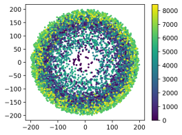
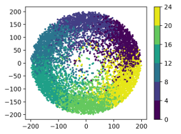
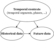
Generally, distribution shift signifies variations in the underlying data generation process, which is typically driven by some temporal observed or unobserved external factors, namely contexts. In this paper, we reveal two significant observed contexts within time series data: temporal segments and periodic phases, along with other unobserved contexts. For example, in the scenario of electricity consumption, factors like economic trends over the years (temporal segments) and seasonal fluctuations (periodic phases) can affect electricity usage. We visualize the influence of the two observed contexts on the distribution of electricity data ETTh1 in Figure 1(a) and 1(b). Moreover, it can also be influenced by the sudden policy changes (unobserved contexts). We refer to this phenomenon as context-driven distribution shift, or CDS in this work.

In the presence of CDS, TSF Transformers remain constrained owing to their ignorance of contexts. Firstly, the training and testing datasets are often generated under distinct contexts (i.e., temporal segments). This deviation from the conventional assumption of consistent dataset distributions between training and testing data can lead to suboptimal prediction results. Secondly, even within the training set, these contexts essentially function as confounders (Pearl, 2009) — factors that simultaneously influence the historical and future data, as demonstrated in Figure 1(c). Such confounders lead trained model to capturing spurious correlations, causing them struggled with generalizing to data from new distributions.

To clearly present the impact of CDS, we trained an Autoformer (Wu et al., 2021) on Illness and assessed its ability to fit sub-data in different periodic phases. Residuals, which reflect the goodness of fitting, were analyzed for the 47th and 32nd periodic phases, as well as for the entire dataset. The residual results are visualized in Figure 1(d). Notably, it can be observed that the model provides an unbiased estimation for the entire training dataset (i.e., the mean of residuals is zero). However, the estimation within two specific contexts is biased owing to their non-zero mean residuals. This observation underscores the model’s limitations in fitting sub-data within a context, as it is susceptible to data from other contexts and learns spurious correlations. It motivates us to calibrate the model to achieve more accurate estimation within each context.

Present work. In this paper, we introduce a general calibration approach to detect and adapt to CDS with a trained model. Specifically, we first propose a metric to measure the severity of model’s susceptibility to CDS within the training data, namely Residual-based context-driven distribution shift detector or Reconditionor, by measuring the mutual information between residuals and observed contexts to quantify the impact of contexts on model’s prediction.

A higher value from Reconditionor signifies a stronger CDS. Under this circumstance, we further propose a simple yet effective adapter framework for further calibration. Given the inherent variability in contexts across data samples, a one-size-fits-all adaptation of the Transformer is inherently unfeasible. Hence, we posit the need to fine-tune the Transformer at the individual sample-level. For each test sample, adapting the model solely based on that single instance is an impractical approach. As an alternative, we initiate a data augmentation process by curating a dataset comprising preceding samples characterized by akin contexts. It is crucial to emphasize that the chosen samples can introduce significant variance during the adaptation process, mainly because of data scarcity. To mitigate this, we restrict the fine-tuning to model’s prediction layer with a limited number of steps. Our theoretical findings substantiate that this fine-tuning framework is able to attains an optimal balance between bias and variance. Moreover, this simple adaptation strategy optimizes model performance while improving processing efficiency. We refer to this framework as Sample-level cOntextuaLIzed aDapter, or SOLID.

Extensive experiments indicate that our proposed calibration approach consistently enhance the performance of five state-of-the-art (SOTA) forecasting Transformers across eight real-world datasets. Notably, our Reconditionor reliably identifies cases requiring CDS adaptation with an accuracy of 90%. Furthermore, our proposed SOLID yields an average improvement ranging from 8.7% to 17.2% when addressing significant CDS situations as detected by Reconditionor. Even in cases with less pronounced CDS, SOLID still achieves an average improvement ranging from 1.1% to 5.9%. Importantly, Reconditionor is highly correlated with the improvement values achieved by SOLID. These findings provide robust validation of the effectiveness of our calibration approach.

The main contributions of this work are summarized as follows:

• We propose the concept of context-driven distribution shift (CDS) by studying the driving factors of distribution shifts, and digest two observed contexts (temporal segments and periodic phases), as well as unobserved contexts.

• We propose a calibration approach, including Reconditionor, a detector to measure the severity of model’s susceptibility to CDS, and SOLID, an adapter to calibrate Transformers for enhancing performance under severe CDS.

• Extensive experiments over various datasets have demonstrated our proposed Reconditionor can detect CDS of forecasting Transformers on the training dataset accurately. Moreover, our proposed SOLID consistently enhance current SOTA Transformers.

2. Related Work

2.1. Time series forecasting Transformers

With the successful rise of Transformers (Vaswani et al., 2017) in natural language processing (NLP) (Devlin et al., 2019) and vision (CV) (Dosovitskiy et al., 2021), increasing Transformer-based models are also proposed for TSF, since the attention mechanism is well-suited for capturing temporal dependencies in time series. And existing Transformer-based forecasting models mainly focus on enhancement in attention by employing sparsity inductive bias or low-rank approximation, hence reducing calculation complexity and better capturing patterns. Specifically, Informer (Zhou et al., 2021) proposes ProbSparse self-attention, Autoformer (Wu et al., 2021) introduces Auto-correlation attention based on seasonal-trend decomposition, FEDformer (Zhou et al., 2022) proposes Fourier frequency enhanced attention, ETSformer (Woo et al., 2022) leverages exponential smoothing attention, and Crossformer (Zhang and Yan, 2023) utilizes a two-stage attention to capture both cross-time and cross-dimension dependency. In this paper, our proposed pipeline can be easily applied to these TSF Transformers.

2.2. Distribution shift in time series

Distribution shift in time series refers to the phenomenon that statistical properties and data distribution continuously vary over time. Specifically, in this paper we highlight that contexts are crucial factors leading to distribution shift, named as context-driven distribution shift. However, how to detect such distribution shift and address it effectively is still a thorny problem.

To better detect such distribution shift, various methods have been proposed. Stephan et al.(Rabanser et al., 2019)  employs dimension reduction and propose a two-sample hypothesis testing. Sean et al. (Kulinski et al., 2020)  proposes an expected conditional distance test statistic and localize the exact feature where distribution shift appears. Lipton et al. (Lipton et al., 2018)  utilizes hypothesis testing based on their proposed Black Box Shift Estimation, thereby detecting the shift. However, these detection methods ignore the important context, and mostly not appropriate for time series data. In contrary, our proposed residual-based detector has sufficient ability to detect the influence of underlying context on distribution shift.

Meanwhile, to address distribution shift in time series forecasting is also crucial, and several researches have explored solutions for the issue. One approach is to employ normalization techniques to stationarize the data. Methods like DAIN (Passalis et al., 2019) employs nonlinear networks to adaptively normalize time series, while RevIN (Kim et al., 2022) proposes a reversible instance normalization to alleviate series shift. AdaRNN (Du et al., 2021) introduces an Adaptive RNN to solve the problem. And Dish-TS (Fan et al., 2023) proposes a Dual-Coefficient Net framework to separately learn the distribution of input and output space, thus capturing their divergence. Another approach involves combining statistical methods with deep networks, e.g., Syml (Smyl, 2019) applies Exponential smoothing on RNN, to concurrently fit seasonality and smoothing coefficients with RNN weights. Additionally, SAF (Arik et al., 2022) integrates a self-supervised learning stage on test samples to train the model before making prediction. However, their method is coupled to model architecture and requires modification of the training process, which limits its application. In contrast, our proposed approach can efficiently adapt the existing models solely during test-time and at sample-level for a better performance.

3. Preliminaries: time series forecasting

For a multi-variate time series with $M$ variables, let ${\bm{x}}_{t}\in\mathbb{R}^{M}$ represent a sample at $t$-th timestep. Given a historical sequence: ${\bm{X}}_{t-L:t}=[{\bm{x}}_{t-L},\cdots,{\bm{x}}_{t-1}]\in\mathbb{R}^{L\times M}$, where $L$ is the look-back window size, the task is to predict future values with $T$ forecasting window size: $\hat{{\bm{X}}}_{t:t+T}=[{\bm{x}}_{t},\cdots,{\bm{x}}_{t+T-1}]\in\mathbb{R}^{T\times M}$. The training objective of a model $f$ is to find the best mapping from input to output sequence, i.e.  $\hat{{\bm{X}}}_{t:t+T}=f({\bm{X}}_{t-L:t})$. In this work, we assume $f$ is a deep neural network composed of two parts: a feature extractor $g_{\Phi}:\mathbb{R}^{L\times M}\rightarrow\mathbb{R}^{d}$ mapping the historical values to a $d$-dimensional latent representation, and a linear top $h_{\theta}$ named as prediction layer mapping the representation to predicted future values.

4. context-driven distribution shift

In this section, we introduce the limitation of traditional TSF Transformers. As mentioned before, the data generation in time series is typically influenced by temporal external factors (i.e., context $c$), such as temporal segments and periodic phases. Let $X$, $Y$ and $C$ denote the variables of historical data ${\bm{X}}_{t-L:t}$, future data ${\bm{X}}_{t:t+T}$ and context $c_{t}$ at time step $t$, respectively. The generation of $Y$ is dependent on $X$ and $C$, characterized as $P(Y\mid X,C)$.

Due to the ignorance of contexts, the model $f$ trained on the dataset actually learns a marginal distribution $P(Y\mid X)=\sum_{c}P(Y\mid X,C=c)P(C=c)$. This introduces a confounding bias (Pearl, 2009) since context $C$ usually influences both the historical data $X$ and the future data $Y$. To illustrate this concept, consider a simplified example in the domain of recommendation. In the winter season (context $C$), users who purchase hot cocoa (historical data $X$) also tend to buy coats (future data $Y$). A model may ”memorize” the correlation between $X$ and $Y$ (a spurious correlation), and mistakenly recommend coats to a user who purchases hot cocoa in summer. This confounding bias leads to suboptimal product recommendations.

Next, we give a formal analysis to show this context-driven distribution shift (CDS) on the latent representation space $g_{\Phi}(\cdot)$. We first make an assumption for the generation process of $Y$:

Assumption 1 (Contextualized generation process).

Assume that the input latent representations $g_{\Phi}(X)$ on the training set can be divided into $K$ context groups based on $K$ different contexts: $(X_{1},\cdots,X_{K})$, where $X_{i}\in\mathbb{R}^{n_{i}\times d}$ and $n_{i}$ is the number of data points in the $i$-th group. For each $i$, there exists a parameter vector $\theta_{i}\in\mathbb{R}^{d}$ such that the output $Y_{i}$ follows:

$$Y_{i}=X_{i}\theta_{i}+\epsilon_{i},$$

where $\epsilon_{i}$ is an independent random noise, which satisfies $\mathbb{E}[\epsilon_{i}]=0$, $\mathbb{VAR}[\epsilon_{i}]=\sigma^{2}$. Here we assume that $Y_{i}$ are scalars for simplicity, although it can be readily extended to a multi-dimensional scenario.

Figure 2. Pipeline of our calibration framework to detect and adapt to context-driven distribution shift (CDS). We leverage \raisebox{-0.9pt}{1}⃝ residual-based context-driven distribution shift detector (Reconditionor) to assess how susceptible a trained model is to CDS. If we detect a significant susceptibility, we employ \raisebox{-0.9pt}{2}⃝ sample-level contextualized adapter (SOLID) to adapt the model for each test sample using preceding data that share similar contexts.

The prediction layer $h_{\theta}$ can be seen as a global linear regressor (GLR) trained on the dataset by mean square error (MSE), as follows:

Definition 0 (Global linear regressor).

A global linear regressor (GLR) $h_{\hat{\theta}}$ parameterized by $\hat{\theta}$ is given by:

$$\hat{\theta}=\arg\min_{\theta}\sum_{i=1}^{K}{||Y_{i}-X_{i}\theta||_{2}^{2}}.$$

Define $\mathcal{R}(\alpha_{1},\cdots,\alpha_{K})=\mathbb{E}\left[\sum_{i=1}^{K}||Y_{i}-X_{i}\alpha_{i}||_{2}^{2}\right]$ as the expected risk when using a parameter $\alpha_{i}$ to predict $X_{i}$ ($i\in[K]$), and let $\mathcal{R}^{*}$ denote the minimum value of this risk. The following theorem computes the expected risk when we use the globally shared parameter for prediction, with its proof delegated to Appendix A.1.

Theorem 2 (Expected risk for GLR).

For $\hat{\theta}$ in Definition 1:

$$\mathcal{R}(\underbrace{\hat{\theta},\cdots,\hat{\theta}}_{K})-\mathcal{R}^{*}=\underbrace{\sum_{i=1}^{K}\left\|\overline{\theta}-\theta_{i}\right\|^{2}_{\psi_{i}}}_{\text{bias part}}+\underbrace{\sigma^{2}d}_{\text{variance part}},$$

where $\psi_{i}=X_{i}^{\top}X_{i}$, and $\overline{\theta}=(\sum_{i=1}^{K}{\psi_{i}})^{-1}(\sum_{i=1}^{K}{\psi_{i}\theta_{i}})$. The quantity $||\cdot||_{\psi_{i}}$ is the Mahalanobis distance norm, defined as $\|\theta\|^{2}_{\psi_{i}}=\theta^{\top}\psi_{i}\theta$.

From the bias part in Theorem 2, it becomes evident that GLR is unbiased only when the data generation parameters $\theta_{i}$ are identical across all groups. However, if they differ due to the influence of contexts, the regressor is biased regardless of the amount of data.

5. Calibration framework for CDS

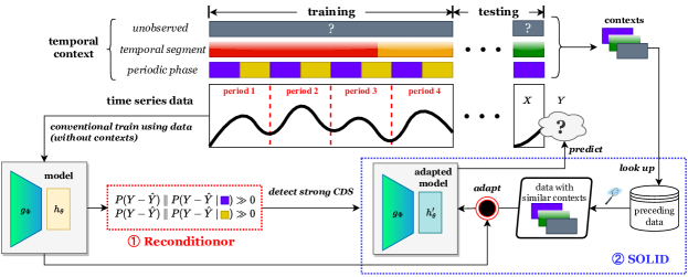
Up to this point, we have demonstrated that a model trained without considering contexts suffering from CDS. In this section, we introduce a general calibration methodology for detecting (in § 5.1) and adapting (in § 5.2) to CDS in conjunction with the model. The pipeline of this calibration framework is illustrated in Figure 2.

5.1. Residual-based CDS detector

Our primary focus lies in assessing the model’s susceptibility to CDS. Our evaluation predominantly centers around observed contexts, as the analysis of unobserved contexts is computationally infeasible. However, for our empirical investigation, the utilization of observed contexts proves to be sufficient.

As previously stated in Theorem 2 and visually demonstrated in Figure 1(d), the presence of contexts introduces a bias to the model estimation, causing variations in residual distributions across different contexts. Based on it, we propose a novel detector, namely Residual-based context-driven distribution shift detector (or Reconditionor), by measuring the mutual information (MI) between prediction residuals and their corresponding contexts. The MI quantifies the extent of information acquired regarding the residuals when observing the context, which serves as a metric for evaluating the influence of contexts on the model. By using the definition of MI (see derivation in Appendix B.1), we have:

(1) $$\delta=\text{MI}(\Delta Y;C)=\mathbb{E}_{C}\left[D_{\text{KL}}\left(P(\Delta Y\mid C)\ \|\ P(\Delta Y)\right)\right],$$

where $\Delta Y=f(X)-Y$ is the residuals of model $f$, and $D_{\text{KL}}(P\|Q)$ is Kullback–Leibler (KL) divergence between distributions $P$ and $Q$.

We reuse Figure 1(d) to illustrate the concept behind Reconditionor when detecting the distribution shift based on the context of periodic phase. The marginal residual distribution $P(\Delta Y)$ typically exhibits a mean close to zero after training. However, the residual distributions conditioned on different contexts (e.g., the 47th phase and the 32th phase) $P(\Delta Y\mid C)$ clearly show non-zero mean values. This increases the KL divergence between the two distributions, consequently elevating $\delta$ and indicating a strong CDS. Additionally, a non-zero mean in the conditional residual distribution suggests the model $f$ fails to adequately fit the data within each context, signaling the need for further adaptation. In summary, a high value of $\delta$ for a model $f$ implies the necessity for adapting $f$, which is also empirically verified in § 6.3.

In practice, we assume that the residuals follow Gaussian distributions. This assumption is based on the utilization of MSE loss, which implicitly presupposes that the residuals adhere to additive Gaussian noise. This characteristic is also evident in Figure 1(d). The adoption of this assumption expedites calculation of KL divergence because Gaussian distributions offer a straightforward analytical solution for it (detailed in Appendix B.2). We illustrate the full algorithm for Reconditionor in Appendix C.1.

5.2. Sample-level contextualized adapter

A higher metric $\delta$ from Reconditionor signifies a stronger impact of CDS on a model. Given the nature of CDS, our primary concept is to adjust the model to align with the conditional distribution $P(Y|X,C)$ instead of the marginal distribution $P(Y|X)$. However, noticing that the context $C$ is consistently changing at each time step, a one-size-fits-all adaptation of the model is inherently unfeasible. Therefore, we propose to carrying out adaptations at the individual sample-level.

For each test sample $X_{t-L:t}$, it is not viable to adapt the model solely relying on the input $X_{t-L:t}$. Therefore, we commence by implementing data augmentation through the creation of a dataset derived from this specific sample, formulated as:

(2) $$\mathcal{D}_{\text{ctx}}=\textsc{Select}(\{({\bm{X}}_{t^{\prime}-L:t^{\prime}},{\bm{X}}_{t^{\prime}:t^{\prime}+T}):t^{\prime}+T\leq t\}),$$

where Select operation involves the selection of preceding samples that share a similar context with the provided sample ${\bm{X}}_{t-L:t}$, and we will provide further elaboration on this operation in § 5.3. We denote the resulting dataset as the contextualized dataset ($\mathcal{D}_{\text{ctx}}$). It’s worth noting that since adaptation takes place during the testing phase, we propose to modify the prediction layer $h_{\theta}$ while keeping the feature extractor $g_{\Phi}$ unchanged, primarily to enhance efficiency.

Before presenting our ultimate adaptation solution, we initially explore a straightforward approach: discarding the existing biased prediction layer $h_{\theta}$ and training a new prediction layer $h^{\prime}_{\theta}$ using $\mathcal{D}_{\text{ctx}}$. In the following we provide a theoretical analysis of this approach. For simplicity, supposing that $\mathcal{D}_{\text{ctx}}$ contains all samples sharing the same context $c$ as the given sample.

As previously demonstrated in § 4, we established that a GLR, which disregards contexts (Definition 1), and is trained on data following a contextualized generation process (Assumption 1), consistently exhibits bias (Theorem 2). Under the same assumption, the aforementioned straightforward solution is equivalent to training an individual regressor $\hat{\theta}_{i}$ for each context group $X_{i}$ ($i\in[K]$) using MSE. We refer to this ensemble of regressors as contextualized linear regressors (CLR), as follows:

Definition 0 (Contextualized linear regressor).

A set of contextualized linear regressors (CLR) $h_{\hat{\theta}_{i}}$ parameterized by $\hat{\theta}_{i}$ ($i\in[K]$) are given by:

$$\hat{\theta}_{i}=\arg\min_{\theta}||Y_{i}-X_{i}\theta||_{2}^{2},\quad\forall i\in\{1,2,...,K\}.$$

Using the same risk notations $\mathcal{R}$ and $\mathcal{R}^{*}$ defined in § 4, the following theorem computes the expected risk for CLR (We defer the proof to Appendix A.2).

Theorem 2 (Expected risk for CLR).

For $\hat{\theta}_{i}$ in Definition 1:

$$\mathcal{R}(\hat{\theta}_{1},\cdots,\hat{\theta}_{K})-\mathcal{R}^{*}=\underbrace{0}_{\text{bias part}}+\underbrace{K\sigma^{2}d}_{\text{variance part}}.$$

Comparing Theorem 2 and Theorem 2, we observe that CLR is always unbiased since it addresses the CDS. However, it suffers from a larger variance compared to GLR. Specifically, the variance of CLR is $K$-times larger than that of GLR, indicating that more detailed contexts result in higher variance. This makes sense because as $K$ increases, the number of data available for training each CLR diminishes, consequently elevating the variance.

Now, we introduce our final solution, namely Sample-level cOntextuaLIzed aDapter, or SOLID. Based on the above findings, we claim that combining GLR and CLR for achieving a better bias-variance trade-off is crucial. This can be implemented through a pre-trained/fine-tuning paradigm. In the pre-training stage, contexts are disregards and a GLR $h_{\theta}$ is trained on the training dataset. Essentially, the pre-training stage mirrors the conventional standard training process. Our proposed SOLID takes effect in the fine-tuning stage. For a given new sample at $t$, we employ $\mathcal{D}_{\text{ctx}}$ to fine-tune the learned GLR for a limited steps. This fine-tuning process brings GLR closer to CLR. In cases where the influence of CDS is substantial (i.e., the bias part in Theorem 2 is large), it is advisable to increase the learning rate and the number of fine-tuning steps to mitigate bias. In the converse case, the fine-tuning process should be more limited to reduce variance, as CLR has greater variance (Theorem 2). In practice, it is recommended to tune the learning hyperparameters to achieve an optimal trade-off between bias and variance.

5.3. Contextualized dataset selection

As we mention previously, the core of adaptation involves creating the contextualized dataset $\mathcal{D}_{\text{ctx}}$ for the sample at $t$. In this section, we introduce the Select operation in Eq.(2). Note that due to the unavailability of the true context governing the data generation process, it is not feasible to select samples with precisely the same context. To address this issue, we design a comprehensive strategy depend on the observable contexts (temporal segments and periodic phases), and employ sample similarity as a proxy for unobserved contexts.

5.3.1. Temporal segments

Data generation process typically evolves over time, illustrated in Figure 1(a). Consequently, we claim that the temporal segment is a critical observed context. Therefore, we focus on samples that are closely aligned with the test samples in the temporal dimension, formally,

$$\{({\bm{X}}_{t^{\prime}-L:t^{\prime}},{\bm{X}}_{t^{\prime}:t^{\prime}+T}):t-\lambda_{T}\leq t^{\prime}\leq t-T\},$$

where $\lambda_{T}$ controls the time range for selection. When samples are too distant from $t$, we conclude that they are in distinct temporal segments and consequently exclude them from selection.

5.3.2. Periodic phases

Furthermore, it’s worth mentioning that time series data often exhibit periodic characteristics. The data generation process can vary across different phases, as exemplified in Figure 1(b). Therefore, we claim that the periodic phase constitutes another critical observed context.

To find the samples with similar phases, we need to detect the underlying periods. Specifically, we follow ETSformer (Woo et al., 2022) and TimesNet (Wu et al., 2023) to employ the widely-used Fast Fourier Transform (FFT) on the training dataset ${\bm{X}}\in\mathbb{R}^{t_{\text{train}}\times M}$ with length-$t_{\text{train}}$ and $M$ variables, formulated as:

(3) $$T^{*}=\Bigl{\lfloor}\nicefrac{{t_{\text{train}}}}{{\left\{\mathop{\arg\max}_{k\in\left\{2,...,\left[\nicefrac{{t_{\text{train}}}}{{2}}\right]\right\}}\sum_{i=1}^{M}\text{Ampl}\left(\text{FFT}\left({\bm{X}}^{i}\right)\right)_{k}\right\}}}\Bigr{\rfloor}.$$

Here, ${\bm{X}}^{i}$ is the sequence of the $i$-th variables in ${\bm{X}}$, $\text{FFT}(\cdot)$ and $\text{Ampl}(\cdot)$ denote the Fast Fourier Transform (FFT) and amplitude respectively. To determine the most dominant frequency, we sum the amplitudes across all $M$ channels and select the highest value, which is converted to the periodic length $T^{*}$.

Next, we employ the periodic length to select samples with closely aligned phases. Particularly, for the given test sample at time step $t^{\prime}$, we select samples that display minimal difference in the phases, formulated as

$$\left\{({\bm{X}}_{t^{\prime}-L:t^{\prime}},{\bm{X}}_{t^{\prime}:t^{\prime}+T}):\left|\frac{t\text{ mod }T^{*}-t^{\prime}\text{ mod }T^{*}}{T^{*}}\right|<\lambda_{P}\right\},$$

where $t\text{ mod }T^{*}$ and $t^{\prime}\text{ mod }T^{*}$ are the phases of the test sample and preceding samples, respectively. $\lambda_{P}$ is a hyperparameter controlling the threshold for the acceptable phase difference. If the difference exceeds the certain threshold, the preceding samples will not be considered to share the same context as the test sample.

5.3.3. Address unobserved contexts through sample similarity

Even though the strategies introduced in § 5.3.1 and § 5.3.2 efficiently identify potential samples with similar contexts, we cannot guarantee a consistent mapping relationship $X\mapsto Y$ for these samples due to the existence of unobserved contexts. To further enhance the quality of selection and address this issue, it’s essential to recognize that context typically influences input data through a causal effect $C\mapsto X$, which suggests a correlation between contexts and inputs.

Inspired by this insight, we assume that when samples have similar inputs $X$, they are more likely to share a similar context $C$. Consequently, we incorporate sample similarity as a proxy of unobserved contexts. The calculation of the similarity can be any measurements of interest, and we employ the Euclidean distance as the chosen metric. Specifically, we select the top-$\lambda_{N}$ similar samples, where $\lambda_{N}$ serves as a hyperparameter governing the number of samples to be chosen.

Table 1. Performance of our proposed methods. ”$\bm{\uparrow}$”: average improvements achieved by SOLID compared to the original forecasting results. ”$\bm{\delta}$”: metrics given by Reconditioner in two observed contexts: periodic phases ($\bm{\delta_{P}}$) and temporal segments ($\bm{\delta_{T}}$), presented in the form of $\bm{\log_{10}\delta_{P}\ \&\ \log_{10}\delta_{T}}$. RED highlights a strong CDS in periodic phases (i.e., $\bm{\log_{10}\delta_{P}\geq-3.2}$), while BLUE highlights a weak CDS in periodic phases (i.e., $\bm{\log_{10}\delta_{P}<-3.2}$).

Method		Crossformer		+SOLID		ETSformer		+SOLID		FEDformer		+SOLID		Autoformer		+SOLID		Informer		+SOLID
Metric		MSE	MAE	MSE	MAE	MSE	MAE	MSE	MAE	MSE	MAE	MSE	MAE	MSE	MAE	MSE	MAE	MSE	MAE	MSE	MAE
Illness	24	3.329	1.275	2.353	0.986	2.397	0.993	2.262	0.955	3.241	1.252	2.707	1.123	3.314	1.245	2.737	1.118	5.096	1.533	2.874	1.150
	36	3.392	1.185	2.527	1.042	2.504	0.970	2.301	0.934	2.576	1.048	2.365	0.990	2.733	1.078	2.540	1.015	5.078	1.535	3.299	1.243
	48	3.481	1.228	2.499	1.063	2.488	0.999	2.320	0.961	2.546	1.058	2.435	1.023	2.651	1.075	2.455	1.042	5.144	1.567	2.879	1.169
	60	3.571	1.234	3.103	1.199	2.494	1.011	2.358	1.002	2.784	1.136	2.677	1.118	2.848	1.126	2.689	1.082	5.243	1.582	3.773	1.394
	$\uparrow$			23.89%	12.84%			6.50%	3.03%			8.64%	5.34%			9.75%	5.90%			37.62%	20.29%
	$\delta$	-1.038 & -0.917				-1.544 & -1.001				-1.099 & -0.917				-1.166 & -1.016				-1.096 & -1.148
Electricity	96	0.184	0.297	0.182	0.295	0.187	0.304	0.171	0.285	0.188	0.304	0.172	0.284	0.207	0.324	0.189	0.304	0.321	0.407	0.245	0.355
	192	0.219	0.317	0.216	0.314	0.198	0.313	0.184	0.298	0.197	0.311	0.180	0.290	0.221	0.334	0.205	0.316	0.351	0.434	0.256	0.363
	336	0.238	0.348	0.235	0.343	0.210	0.326	0.197	0.312	0.213	0.328	0.195	0.307	0.244	0.350	0.232	0.337	0.349	0.432	0.279	0.381
	720	0.274	0.373	0.269	0.368	0.249	0.356	0.234	0.341	0.243	0.352	0.228	0.336	0.285	0.381	0.273	0.370	0.385	0.493	0.327	0.416
	$\uparrow$			1.42%	1.11%			6.89%	4.75%			7.88%	5.95%			6.16%	4.44%			21.28%	14.21%
	$\delta$	-2.333 & -2.42				-2.559 & -2.724				-2.967 & -2.545				-2.408 & -2.134				-2.975 & -2.593
Traffic	96	0.521	0.297	0.473	0.277	0.599	0.386	0.487	0.354	0.574	0.356	0.513	0.344	0.621	0.391	0.565	0.376	0.731	0.406	0.628	0.393
	192	0.523	0.298	0.475	0.280	0.611	0.391	0.492	0.354	0.612	0.379	0.549	0.361	0.666	0.415	0.599	0.379	0.739	0.414	0.653	0.413
	336	0.530	0.300	0.481	0.286	0.619	0.393	0.501	0.359	0.618	0.379	0.557	0.363	0.649	0.405	0.595	0.390	0.850	0.476	0.758	0.466
	720	0.573	0.313	0.498	0.298	0.629	0.391	0.529	0.374	0.629	0.382	0.577	0.371	0.684	0.422	0.635	0.411	0.945	0.530	0.861	0.524
	$\uparrow$			10.25%	5.55%			18.28%	7.57%			9.77%	3.70%			8.61%	4.80%			11.19%	1.65%
	$\delta$	-2.879 & -2.171				-2.488 & -2.201				-2.254 & -2.265				-2.507 & -2.304				-2.762 & -2.238
ETTh1	96	0.411	0.432	0.382	0.415	0.495	0.480	0.491	0.478	0.375	0.414	0.370	0.410	0.440	0.444	0.430	0.442	0.948	0.774	0.684	0.586
	192	0.419	0.444	0.396	0.422	0.543	0.505	0.538	0.503	0.427	0.448	0.420	0.443	0.487	0.472	0.480	0.470	1.009	0.786	0.759	0.624
	336	0.439	0.459	0.418	0.443	0.581	0.521	0.574	0.518	0.458	0.465	0.454	0.462	0.471	0.475	0.467	0.473	1.035	0.783	0.776	0.640
	720	0.504	0.514	0.473	0.503	0.569	0.534	0.562	0.530	0.482	0.495	0.478	0.492	0.543	0.528	0.542	0.527	1.153	0.845	0.948	0.726
	$\uparrow$			5.94%	3.53%			1.08%	0.56%			1.10%	0.74%			1.08%	0.35%			23.60%	19.18%
	$\delta$	-3.111 & -2.767				-3.207 & -3.019				-3.52 & -2.463				-3.572 & -2.321				-3.83 & -1.883
ETTh2	96	0.641	0.555	0.527	0.544	0.346	0.401	0.344	0.399	0.341	0.385	0.339	0.383	0.363	0.405	0.362	0.404	2.992	1.362	0.948	0.727
	192	1.262	0.814	0.834	0.725	0.437	0.447	0.430	0.443	0.433	0.441	0.432	0.440	0.450	0.447	0.449	0.446	6.256	2.091	1.791	1.056
	336	1.486	0.896	1.048	0.835	0.478	0.479	0.467	0.472	0.503	0.494	0.501	0.491	0.470	0.474	0.468	0.471	5.265	1.954	1.845	1.079
	720	1.220	0.848	0.906	0.758	0.488	0.492	0.474	0.482	0.479	0.485	0.478	0.484	0.484	0.491	0.483	0.489	4.038	1.673	2.020	1.104
	$\uparrow$			28.05%	8.06%			1.93%	1.31%			0.42%	0.40%			0.25%	0.35%			64.40%	44.00%
	$\delta$	-2.451 & -1.149				-3.067 & -1.079				-3.733 & -1.943				-3.967 & -1.921				-3.021 & -1.513

• Results of ETTm1, ETTm2 and Weather datasets are included in Table 5 of Appendix E, due to space limit.

5.3.4. Full algorithm for SOLID

Finally, we combine the above strategies for the Select operation, by first filtering the temporal segments and periodic phases (§ 5.3.1 and § 5.3.2) and then select top-$\lambda_{N}$ samples based on similarity (§ 5.3.3). We illustrate the full algorithm for SOLID in Appendix C.2.

6. Experiments

In this section, we describe the experimental settings and provide extensive results and analysis.

6.1. Experiment settings

Datasets. We conduct the experiments on 8 popular datasets for TSF: Electricity, Traffic, Illness, Weather (Lai et al., 2018), and 4 ETT datasets (ETTh1, ETTh2, ETTm1, ETTm2) (Zhou et al., 2021). We follow the standard preprocessing protocol (Zhou et al., 2021; Wu et al., 2021) and partition the datasets into train/validation/test sets by the ratio of 6:2:2 for ETT and 7:1:2 for the other datasets. Appendix D.1 contains more dataset details.

Baseline models. As aforementioned, our proposed approach is a general framework which can make calibration on many deep forecasting Transformer models. To verify the effectiveness, we select five SOTA multi-variate Transformer-based forecasting models for detection and adaptation, including Crossformer (Zhang and Yan, 2023), ETSformer (Woo et al., 2022), FEDformer (Zhou et al., 2022), Autoformer (Wu et al., 2021), and Informer (Zhou et al., 2021). Appendix D.2 contains more details about the baselines.

Experimental details. For a fair comparison, we set the forecasting window length $T$ of {24,36,48,60} for Illness dataset, and {96,192,336,720} for the others, which aligns with the commonly adopted setting for TSF tasks (Wu et al., 2021; Zhou et al., 2022). Additionally, for other hyper-parameters, we follow the primary settings proposed in each respective paper (Zhang and Yan, 2023; Woo et al., 2022; Zhou et al., 2022; Wu et al., 2021; Zhou et al., 2021). For our SOLID, we employ gradient descent to fine-tune the prediction layer on $\mathcal{D}_{\text{ctx}}$ for one epoch. Appendix D.3 contains more details about the hyper-parameters.

Evaluation metrics. Consistent with previous researches (Zhou et al., 2021; Wu et al., 2021; Zhou et al., 2022), we compare the performance via two widely-used metrics: Mean Squared Error (MSE) and Mean Absolute Error (MAE). Smaller MSE and MAE indicate better forecasting performance. We also compute the proposed Reconditionor as metrics for detecting the extend of models’ susceptibility to CDS based on the two observed contexts, periodic phase ($\delta_{P}$) and temporal segment ($\delta_{T}$). For $\delta_{P}$, the number of contexts equals to the periodic length, detailed in Eq.(3). For $\delta_{T}$, we partition the training set into five equal segments, with each one representing a distinct temporal segment. Larger $\delta_{P}$ and $\delta_{T}$ indicate a stronger CDS for the given model and dataset.

6.2. Main results analysis

Table 1 shows the main results of our proposed SOLID alongside the scores of the proposed Reconditionor. We conduct a thorough analysis of the data from both perspectives.

6.2.1. Effectiveness of SOLID

1. SOLID enhances the performance of all models across various datasets by effectively addressing the CDS issue. Particularly, Informer, which is relatively less powerful, experiences a significant enhancement of 10%-60% in MSE. One explanation is that CDS has a more detrimental effect on weaker models, as they struggle to learn diverse patterns under different contexts.

2. For datasets and models showing significant CDS under the context of periodic phases (i.e., $\log_{10}\delta_{P}$ exceeding the $-3.2$ threshold), SOLID achieves a considerable improvement. Specifically, it yields an average improvement of 11.6% for Traffic, 8.7% for Electricity, and 17.2% for Illness in terms of MSE. This highlights the effectiveness of SOLID in addressing severe CDS issues.

3. On the cases of weak CDS under the context of periodic phases (i.e., $\log_{10}\delta_{P}$ below the $-3.2$ threshold), SOLID still achieves a consistent improvement ranging from 1.1% to 5.9%. This observation underscores the widespread presence of CDS in time series.

6.2.2. Effectiveness of Reconditionor

1. Our Reconditionor effectively assesses the magnitude of CDS and and aligns with the enhancement achieved by SOLID. When employing the $-3.2$ threshold for $\log_{10}\delta_{P}$ to ascertain whether MAE improvement surpasses 1%, the classification accuracy reaches 90% (36 out of 40). This finding demonstrates that this detector is universally applicable, unaffected by variations in dataset size and model implementation.

2. One exception is that Informer consistently achieves an improvement above 1%, irrespective of Reconditionor metrics. As aforementioned, one explanation is that Informer is relatively weaker, making it more amenable to improvement by SOLID. When the results of Informer are excluded, the classification accuracy for Reconditionor rises to 96.88% (31 out of 32).

3. In addition, $\delta_{P}$ explains the performance improvement better than $\delta_{T}$. We will give a possible conjecture in the following subsection to elucidate this observation.

(a) periodic phases ($\delta_{P}$)

(b) temporal segments ($\delta_{T}$)

Figure 3. The relationship of Reconditionor metrics $\bm{\log_{10}\delta_{P}}$ and $\bm{\log_{10}\delta_{T}}$ (X-axis) and MAE improvements achieved by SOLID (Y-axis) for eight datasets and four models.

6.3. Correlation of Reconditionor and SOLID

To further investigate the correlation between Reconditioner and the improvements achieved by SOLID, we plot $\delta_{P}$, $\delta_{T}$ and MAE improvements in Figure 3 based on the results of Table 1 and Table 5 in Appendix E. To depict the trend more effectively, we have excluded the data of Informer as previously explained.

Notably, we have observed a pronounced and consistent upward trend between $\delta_{P}$ and MAE improvement in Figure 3(a). This trend is highly evident, with a Spearman correlation coefficient of 0.814. This finding indicates that the enhancements achieved by SOLID predominantly stem from its ability to address CDS issue caused by distinct periodic phases. It suggests that $\delta_{P}$ can serve as a valuable metric for estimating performance improvements.

However, the relation between $\delta_{T}$ and MAE improvement is not as straightforward. Despite showing an increasing trend in Figure 3(b), the Spearman correlation coefficient is merely 0.162. This implies that, while there is evidence of CDS stemming from temporal segments as detected by Reconditionor, SOLID is comparatively less effective at mitigating it when compared to CDS caused by periodic phases. One possible explanation is that data generated within the same phase tends to follow a more predictable pattern, while data within the same temporal segment exhibits greater diversity and uncertainty, which may limit the utility of selecting data from the same segment to address CDS caused by temporal segments. We leave further investigation of it to future work.

Figure 4. The influence of different parameter $\lambda_{T}$, $\lambda_{P}$, $\lambda_{N}$ and $lr$ settings on the MSE performance on Illness and Traffic dataset.

(a) Illness-$\lambda_{T}$

(b) Traffic-$\lambda_{T}$

(c) Illness-$\lambda_{P}$

(d) Traffic-$\lambda_{P}$

(e) Illness-$\lambda_{N}$

(f) Traffic-$\lambda_{N}$

(g) Illness-$lr$

(h) Traffic-$lr$

6.4. Ablation study for SOLID

In this section, we conduct an ablation study, aiming to investigate the relationship between performance and each components in the selection strategy, as our strategy is designed to select from preceding samples that share the most similar contexts, relying on temporal segments, periodic phases, and sample similarity.

The investigation involves a progression of strategy components, which is presented in Table 2. Specifically, we commence from original forecasts that ignore any contexts, denoted as ”/”. We then create contextualized datasets with various selection variations. For a fair comparison, all datasets are constructed by selecting $\lambda_{N}$ samples from $\lambda_{T}$ nearest ones. We first consider Temporal segment context by selecting the nearest $\lambda_{N}$ samples, denoted as ”T”. Then we take Periodic phase into consideration, and select $\lambda_{N}$ nearest samples with phase differences less than $\lambda_{P}$, denoted as ”T+P”. Finally, we add sample Similarity and select the top-$\lambda_{N}$ similar samples from nearest $\lambda_{T}$ samples with phase differences less than $\lambda_{P}$. This strategy is consistent with SOLID, and is denoted as ”T+P+S”. Based on the results in Table 2, we showcase that each component leads to a consistent improvement in both MSE and MAE. These findings provide compelling evidence supporting the effectiveness of all components utilized in our selection strategy as well as the SOLID method.

Table 2. Ablation study on SOLID.

Dataset		Electricity		Traffic		Illness
Metric		MSE	MAE	MSE	MAE	MSE	MAE
Informer	/	0.321	0.407	0.731	0.406	5.106	1.534
	T	0.252	0.362	0.636	0.396	4.443	1.427
	T+P	0.248	0.358	0.628	0.393	2.901	1.186
	T+P+S	0.245	0.355	0.628	0.393	2.874	1.150
Autoformer	/	0.207	0.324	0.620	0.391	3.314	1.245
	T	0.193	0.309	0.579	0.380	3.333	1.251
	T+P	0.196	0.309	0.577	0.380	2.981	1.201
	T+P+S	0.189	0.304	0.565	0.377	2.737	1.118
FEDformer	/	0.188	0.304	0.574	0.356	3.241	1.252
	T	0.173	0.284	0.522	0.346	3.234	1.253
	T+P	0.172	0.283	0.520	0.345	2.953	1.189
	T+P+S	0.172	0.284	0.513	0.344	2.707	1.123
ETSformer	/	0.187	0.304	0.599	0.386	2.397	0.993
	T	0.174	0.289	0.493	0.356	2.377	0.989
	T+P	0.173	0.287	0.489	0.356	2.334	0.977
	T+P+S	0.171	0.285	0.487	0.354	2.262	0.955
Crossformer	/	0.184	0.297	0.521	0.297	3.329	1.275
	T	0.188	0.301	0.482	0.273	2.705	1.098
	T+P	0.184	0.297	0.476	0.270	2.469	0.993
	T+P+S	0.182	0.295	0.473	0.267	2.353	0.986

6.5. Parameter sensitivity analysis

Within our proposed approach, several crucial parameters are presented, including: $\lambda_{T}$, which controls the time range of preceding data for selection; $\lambda_{P}$, which governs the acceptable threshold for periodic phase difference; $\lambda_{N}$, which determines the number of similar samples to be selected for model adaptation; And $lr$, which regulates the extent of adaptation on the prediction layer for the models. The search range for these parameters are presented in Table 4 in Appendix D.3. And the results of parameter sensitivity analysis are visually presented in Figure 5(h).

Firstly, we discover that our proposed SOLID is insensitive to $\lambda_{T}$ and $\lambda_{P}$ parameters, based on the results obtained. Regarding $\lambda_{N}$ parameter, the selection of insufficient samples would increase the variance during adaptation due to the data shortage. Conversely, selecting excessive samples carries the risk of including samples with unobserved irrelevant contexts, thereby deteriorating model’s performance. Lastly, For parameter $lr$, a very small $lr$ leads to inadequate model adaptation, preventing the model from effectively addressing CDS and resulting in a bias towards the test sample (Theorem 2). Conversely, a too large value for $lr$ can lead to excessive adaptation, which also risks in bringing in substantial variance to the model (Theorem 2). Therefore, a well-selected learning rate will contribute to an optimal trade-off between bias and variance.

6.6. Other experiments

Additionally, we conduct a case study for visualizing the improvement, and a comparison experiment between adaptation on prediction layer versus adaptation on the entire model. These results are presented in Appendix F and G due to space limit.

7. Conclusion

In this paper, we introduce context-driven distribution shift (CDS) problem in TSF and identify two significant observed contexts, including temporal segments and periodic phases, along with unobserved contexts. To address the issue, we propose a general calibration framework, including a detector, Reconditionor, to evaluate the degree of a model’s susceptibility to CDS and the necessity for model adaptation; and an adaptation framework, SOLID, for calibrating models and enhancing their performance under severe CDS. We conduct extensive experiments on various real-world datasets, demonstrating the accuracy of Reconditionor in detecting CDS and the effectiveness of SOLID in adapting TSF Transformers. This adaptation consistently leads to improved performance.

Future work. As we discussed in § 6.3, SOLID appears to be less effective in mitigating CDS from temporal segments, compared to its remarkable performance in addressing CDS from periodic phases. This discrepancy may be attributed to the higher level of uncertainty within the same temporal segment. We leave how to better address the CDS from temporal segments as future work.

Appendix

Appendix A Proofs for the theoretical results

In this section, we give the proofs for the expected risks in Theorem 2 and Theorem 2. To start with, we give the following lemma to perform the usual bias/variance decomposition. The risk notations $\mathcal{R}$ and $\mathcal{R}^{*}$ are defined in § 4.

Lemma A.0 (Risk decomposition).

For a set of random variables $\alpha_{1},\cdots,\alpha_{K}$ used as parameters for each group, we have:

$$\mathcal{R}(\alpha_{1},\cdots,\alpha_{K})-\mathcal{R^{*}}=\underbrace{\sum_{i=1}^{K}\left\|\mathbb{E}[\alpha_{i}]-\theta_{i}\right\|^{2}_{\psi_{i}}}_{\text{bias part}}+\underbrace{\sum_{i=1}^{K}\mathbb{E}\left[\left\|\alpha_{i}-\mathbb{E}[\alpha_{i}]\right\|^{2}_{\psi_{i}}\right]}_{\text{variance part}},$$

where $\psi_{i}=X_{i}^{\top}X_{i}$, $\overline{\theta}=(\sum_{i=1}^{K}{\psi_{i}})^{-1}(\sum_{i=1}^{K}{\psi_{i}\theta_{i}})$, and $\|\theta\|^{2}_{\psi_{i}}=\theta^{\top}\psi_{i}\theta$.

Proof.

This is a direct corollary of Proposition 3.3 in (Bach, 2023). ∎

Based on the risk decomposition, we give the computation for GLR and CLR respectively, as follows.

A.1. Proof for Theorem 2

Set $\alpha_{1}=\cdots=\alpha_{K}=\hat{\theta}$ in Lemma 1, we obtain:

$$\mathcal{R}\underbrace{\left(\hat{\theta},\cdots,\hat{\theta}\right)}_{K}-\mathcal{R^{*}}=\underbrace{\sum_{i=1}^{K}\left\|\mathbb{E}[\hat{\theta}]-\theta_{i}\right\|^{2}_{\psi_{i}}}_{\text{bias part}}+\underbrace{\sum_{i=1}^{K}\mathbb{E}\left[\left\|\alpha_{i}-\mathbb{E}[\hat{\theta}]\right\|^{2}_{\psi_{i}}\right]}_{\text{variance part}}.$$

We first compute the expectation in the bias part. Recall that,

$$\hat{\theta}=\arg\min_{\theta}\sum_{i=1}^{K}\|Y_{i}-X_{i}\theta\|_{2}^{2},$$

which has a closed-form solution, as follows:

(A.1) $$\hat{\theta}=\left(\sum_{i=1}^{K}\psi_{i}\right)^{-1}\left(\sum_{i=1}^{K}X_{i}^{\top}Y_{i}\right)=\left(\sum_{i=1}^{K}\psi_{i}\right)^{-1}\left(\sum_{i=1}^{K}X_{i}^{\top}(X_{i}\theta_{i}+\epsilon_{i})\right).$$

Therefore, we can obtain the expectation:

$$\mathbb{E}[\hat{\theta}] =\left(\sum_{i=1}^{K}\psi_{i}\right)^{-1}\left(\sum_{i=1}^{K}X_{i}^{\top}(X_{i}\theta_{i}+\mathbb{E}[\epsilon_{i}])\right)$$

(A.2) $$=\left(\sum_{i=1}^{K}\psi_{i}\right)^{-1}\left(\sum_{i=1}^{K}\psi_{i}\theta_{i}\right):=\overline{\theta},$$

which implies the bias part. Then we compute the variance part $V$:

$$V =\sum_{i=1}^{K}\mathbb{E}\left[\left\|\hat{\theta}-\mathbb{E}[\hat{\theta}]\right\|^{2}_{\psi_{i}}\right]$$

$$=\sum_{i=1}^{K}\mathbb{E}\left[\left\|\left(\sum_{j=1}^{K}\psi_{j}\right)^{-1}\left(\sum_{j=1}^{K}X_{j}^{\top}\epsilon_{j}\right)\right\|^{2}_{\psi_{i}}\right]\cdots\text{by Eq.(\ref{eq:thm1_hat_theta}) and Eq.(\ref{eq:thm1_e_hat_theta})}$$

$$=\sum_{i=1}^{K}\mathbb{E}\left[\left(\sum_{j=1}^{K}X_{j}^{\top}\epsilon_{j}\right)^{\top}\underbrace{\left(\sum_{j=1}^{K}\psi_{j}\right)^{-1}\psi_{i}\left(\sum_{j=1}^{K}\psi_{j}\right)^{-1}}_{\text{denoted by }P_{i}}\left(\sum_{j=1}^{K}X_{j}^{\top}\epsilon_{j}\right)\right]$$

$$=\sum_{i=1}^{K}\mathbb{E}\left[\left(\sum_{j=1}^{K}X_{j}^{\top}\epsilon_{j}\right)^{\top}P_{i}\left(\sum_{j=1}^{K}X_{j}^{\top}\epsilon_{j}\right)\right]$$

$$=\sum_{i=1}^{K}\mathbb{E}\left[\left(\sum_{j=1}^{K}\epsilon_{j}^{\top}X_{j}\right)P_{i}\left(\sum_{j=1}^{K}X_{j}^{\top}\epsilon_{j}\right)\right]$$

$$=\sum_{i=1}^{K}\mathbb{E}\left[\sum_{j=1}^{K}\sum_{k=1}^{K}\epsilon_{j}^{\top}X_{j}P_{i}X_{k}^{\top}\epsilon_{k}\right]$$

$$=\sum_{i=1}^{K}\sum_{j=1}^{K}\sum_{k=1}^{K}\mathbb{E}\left[\epsilon_{j}^{\top}X_{j}P_{i}X_{k}^{\top}\epsilon_{k}\right]$$

$$=\sum_{i=1}^{K}\sum_{j=1}^{K}\mathbb{E}\left[\epsilon_{j}^{\top}X_{j}P_{i}X_{j}^{\top}\epsilon_{j}\right]\cdots\text{by }\mathbb{E}[\epsilon_{j}^{\top}X_{j}P_{i}X_{k}^{\top}\epsilon_{k}]=0\text{ if }j\neq k$$

$$=\sum_{i=1}^{K}\sum_{j=1}^{K}\mathbb{E}\left[\text{tr}(X_{j}P_{i}X_{j}^{\top}\epsilon_{j}\epsilon_{j}^{\top})\right]\cdots\text{by tr}(AB)=\text{tr}(BA)$$

$$=\sigma^{2}\sum_{i=1}^{K}\sum_{j=1}^{K}\text{tr}(X_{j}P_{i}X_{j}^{\top})\cdots\text{by }\mathbb{E}[\epsilon_{j}\epsilon_{j}^{\top}]=\sigma^{2}I_{n}$$

$$=\sigma^{2}\sum_{i=1}^{K}\sum_{j=1}^{K}\text{tr}\left(X_{j}\left(\sum_{k=1}^{K}\psi_{k}\right)^{-1}\psi_{i}\left(\sum_{k=1}^{K}\psi_{k}\right)^{-1}X_{j}^{\top}\right)\cdots\text{by plugging }P_{i}$$

$$=\sigma^{2}\sum_{i=1}^{K}\sum_{j=1}^{K}\text{tr}\left(\psi_{j}\left(\sum_{k=1}^{K}\psi_{k}\right)^{-1}\psi_{i}\left(\sum_{k=1}^{K}\psi_{k}\right)^{-1}\right)\cdots\text{by }\psi_{j}=X_{j}^{\top}X_{j}$$

$$=\sigma^{2}\text{tr}\left(\sum_{i=1}^{K}\sum_{j=1}^{K}\psi_{j}\left(\sum_{k=1}^{K}\psi_{k}\right)^{-1}\psi_{i}\left(\sum_{k=1}^{K}\psi_{k}\right)^{-1}\right)$$

$$=\sigma^{2}\text{tr}\left(\left(\sum_{j=1}^{K}\psi_{j}\right)\left(\sum_{k=1}^{K}\psi_{k}\right)^{-1}\left(\sum_{i=1}^{K}\psi_{i}\right)\left(\sum_{k=1}^{K}\psi_{k}\right)^{-1}\right)$$

$$=\sigma^{2}\text{tr}(I\cdot I)$$

$$=\sigma^{2}d.$$

A.2. Proof for Theorem 2

Set $\alpha_{i}=\hat{\theta}_{i}$ in Lemma 1 for $i\in[K]$, we obtain:

(A.3) $$\mathcal{R}\left(\hat{\theta}_{1},\cdots,\hat{\theta}_{K}\right)-\mathcal{R^{*}}=\underbrace{\sum_{i=1}^{K}\left\|\mathbb{E}[\hat{\theta}_{i}]-\theta_{i}\right\|^{2}_{\psi_{i}}}_{\text{bias part}}+\underbrace{\sum_{i=1}^{K}\mathbb{E}\left[\left\|\hat{\theta}_{i}-\mathbb{E}[\hat{\theta}_{i}]\right\|^{2}_{\psi_{i}}\right]}_{\text{variance part}}.$$

From Proposition 3.4 and Proposition 3.5 in (Bach, 2023), for each $i\in[K]$:

(A.4) $$\left\|\mathbb{E}[\hat{\theta}_{i}]-\theta_{i}\right\|^{2}_{\psi_{i}}=0,\quad\mathbb{E}\left[\left\|\hat{\theta}_{i}-\mathbb{E}[\hat{\theta}_{i}]\right\|^{2}_{\psi_{i}}\right]=\sigma^{2}d.$$

Combining Eq.(A.3) and Eq.(A.4), we obtain the desired result.

Appendix B Further details in Reconditionor

We provide further details in the proposed Reconditionor, including the derivation of MI and the KL divergences between Gaussian distributions.

B.1. Derivation of MI

We provide detailed derivation for Eq.(1). Let $\Delta Y=f(X)-Y$ denote residuals. Mutual information between residual $\Delta Y$ and context $C$ is the KL divergence from the product of the marginal distributions $P(\Delta Y)\cdot P(C)$, of the joint distribution $P(\Delta Y,C)$. Therefore:

$$\delta =\text{MI}(\Delta Y;C)$$

$$=D_{\text{KL}}\left(P(\Delta Y,C)\ \|\ P(\Delta Y)P(C)\right)$$

$$=\sum_{c\in\mathcal{C}}\sum_{\Delta y\in\mathcal{Y}}P(\Delta y,c)\log\frac{P(\Delta y,c)}{P(\Delta y)P(c)}$$

$$=\sum_{c\in\mathcal{C}}\sum_{\Delta y\in\mathcal{Y}}P(\Delta y\mid c)P(c)\log\frac{P(\Delta y\mid c)P(c)}{P(\Delta y)P(c)}$$

$$=\sum_{c\in\mathcal{C}}P(c)\sum_{\Delta Y\in\mathcal{Y}}P(\Delta y\mid c)\log\frac{P(\Delta y\mid c)}{P(\Delta y)}$$

$$=\sum_{c\in\mathcal{C}}P(c)D_{\text{KL}}(P(\Delta Y\mid C=c)\ \|\ P(\Delta Y))$$

$$=\mathbb{E}_{C}\left[D_{\text{KL}}\left(P(\Delta Y\mid C)\ \|\ P(\Delta Y)\right)\right],$$

where $\mathcal{C}$ and $\mathcal{Y}$ are the ranges of context $C$ and residual $\Delta Y$, respectively.

B.2. Derivation of KL divergence between Gaussian distributions

Suppose $P=\mathcal{N}(\mu_{1},\sigma_{1}^{2})$ and $Q=\mathcal{N}(\mu_{2},\sigma_{2}^{2})$, we calculate the KL divergence between them to provide an analytical solution for Reconditionor as follows:

$$\text{KL}= \int\left[\log(P(x))-\log(Q(x))\right]P(x)dx$$

$$= \int\left[-\frac{1}{2}\log(2\pi)-\log(\sigma_{1})-\frac{1}{2}\left(\frac{x-\mu_{1}}{\sigma_{1}}\right)^{2}+\frac{1}{2}\log(2\pi)+\right.$$

$$\left.\log(\sigma_{2})+\frac{1}{2}\left(\frac{x-\mu_{2}}{\sigma_{2}}\right)^{2}\right]\times\frac{1}{\sqrt{2\pi}\sigma_{1}}\exp\left[-\frac{1}{2}\left(\frac{x-\mu_{1}}{\sigma_{1}}\right)^{2}\right]dx$$

$$= \int\left\{\log\left(\frac{\sigma_{2}}{\sigma_{1}}\right)+\frac{1}{2}\left[\left(\frac{x-\mu_{2}}{\sigma_{2}}\right)^{2}-\left(\frac{x-\mu_{1}}{\sigma_{1}}\right)^{2}\right]\right\}\times$$

$$\frac{1}{\sqrt{2\pi}\sigma_{1}}\exp\left[-\frac{1}{2}\left(\frac{x-\mu_{1}}{\sigma_{1}}\right)^{2}\right]dx$$

$$= \mathbb{E}_{P}\left\{\log\left(\frac{\sigma_{2}}{\sigma_{1}}\right)+\frac{1}{2}\left[\left(\frac{x-\mu_{2}}{\sigma_{2}}\right)^{2}-\left(\frac{x-\mu_{1}}{\sigma_{1}}\right)^{2}\right]\right\}$$

$$= \log\left(\frac{\sigma_{2}}{\sigma_{1}}\right)+\frac{1}{2\sigma_{2}^{2}}\mathbb{E}_{P}\left\{(x-\mu_{2})^{2}\right\}-\frac{1}{2\sigma_{1}^{2}}\mathbb{E}_{P}\left\{(x-\mu_{1})^{2}\right\}$$

$$= \log\left(\frac{\sigma_{2}}{\sigma_{1}}\right)+\frac{1}{2\sigma_{2}^{2}}\mathbb{E}_{P}\left\{(x-\mu_{2})^{2}\right\}-\frac{1}{2}$$

$$= \log\left(\frac{\sigma_{2}}{\sigma_{1}}\right)+\frac{1}{2\sigma_{2}^{2}}\left[\mathbb{E}_{P}\left\{(x-\mu_{1})^{2}\right\}+(\mu_{1}-\mu_{2})^{2}\right]-\frac{1}{2}$$

$$= \log\left(\frac{\sigma_{2}}{\sigma_{1}}\right)+\frac{\sigma_{1}^{2}+(\mu_{1}-\mu_{2})^{2}}{2\sigma_{2}^{2}}-\frac{1}{2}.$$

Appendix C Algorithms

Input: Model $f$, training data with $K$ contexts $\mathcal{D}^{\text{train}}=\{({\bm{X}}_{t-L:t},{\bm{X}}_{t:t+T},c_{t}):t<t_{\text{train}},c_{t}\in[K]\}$.

Output: $\delta\in[0,1]$ indicating $f$’s susceptibility to CDS.

1 $R\leftarrow\varnothing$;

2 $R_{1},\cdots,R_{K}\leftarrow\varnothing,\cdots,\varnothing$;

3 for $L\leq t<t_{\text{train}}$ do

4       $r\leftarrow f({\bm{X}}_{t-L:t})-{\bm{X}}_{t:t+T}$;

5       $R\leftarrow R\cup r$;

6       $R_{c_{t}}\leftarrow R_{c_{t}}\cup r$;

7      

8 end for

9$\mu,\sigma\leftarrow\text{Mean}(R),\text{Standard-Deviation}(R)$;

10 $\delta\leftarrow 0$;

11 for $c\in[K]$ do

12       $\mu_{c},\sigma_{c}\leftarrow\text{Mean}(R_{c}),\text{Standard-Deviation}(R_{c})$;

13       $\delta\leftarrow\delta+\frac{|R_{c}|}{|R|}\text{KL}(\mathcal{N}(\mu_{c},\sigma_{c}^{2})\ \|\ \mathcal{N}(\mu,\sigma^{2}))$;

14      

15 end for

16return $\delta$;

Algorithm 1 Algorithm for Reconditionor

Input: Model $f=(g_{\Phi},h_{\theta})$, test sample ${\bm{X}}_{t-L:t}$, preceding data $\{({\bm{X}}_{t^{\prime}-L:t^{\prime}},{\bm{X}}_{t^{\prime}:t^{\prime}+T}):t^{\prime}+T\leq t\}$, similarity metric $S(\cdot,\cdot)$, periodic length $T^{*}$ computed by Eq.(3), hyperparameters $\lambda_{T}$, $\lambda_{P}$, $\lambda_{N}$ and $lr$.

Output: Prediction for the test sample: $\hat{\bm{X}}_{t:t+T}$

1 $\mathcal{T}\leftarrow\varnothing$;

2 for $t-\lambda_{T}\leq t^{\prime}\leq t-T$ do

3       $\Delta_{P}\leftarrow\left|\frac{t\text{ mod }T^{*}-t^{\prime}\text{ mod }T^{*}}{T^{*}}\right|$;

4       if $\Delta_{P}<\lambda_{P}$ then

5             $\mathcal{T}\leftarrow\mathcal{T}\cup\{t^{\prime}\}$;

6            

7       end if

8      

9 end for

10$\mathcal{T}_{\text{ctx}}\leftarrow\mathop{\text{argTop-}\lambda_{N}}\limits_{t^{\prime}\in\mathcal{T}}(S({\bm{X}}_{t^{\prime}-L:t^{\prime}},{\bm{X}}_{t-L:t}))$;

11 $\mathcal{D}_{\text{ctx}}\leftarrow\{({\bm{X}}_{t^{\prime}-L:t^{\prime}},{\bm{X}}_{t^{\prime}:t^{\prime}+T})\mid t\in\mathcal{T}_{\text{ctx}}\}$;

12 $h_{\theta}^{\prime}\leftarrow$ fine-tune $h_{\theta}$ using $\mathcal{D}_{\text{ctx}}$ with a learning rate $lr$;

13 $\hat{\bm{X}}_{t:t+T}\leftarrow h_{\theta}^{\prime}(g_{\Phi}({\bm{X}}_{t-L:t}))$;

14 return $\hat{\bm{X}}_{t:t+T}$;

Algorithm 2 Algorithm for SOLID

C.1. Full algorithm for Reconditionor

Algorithm 1 illustrates the full procedure for Reconditionor. In lines 1-2, we initialize the sets of residuals for both the marginal distribution $P(\Delta Y)$ and the conditional distributions $P(\Delta Y\mid C)$ for each $C\in[K]$. In lines 3-7, we update these sets with the residuals computed by $f$. We compute the mean and standard deviation values for $P(\Delta Y)$ in line 8 and perform a similar computation for $P(\Delta Y\mid C)$ in line 11. Finally, in line 12, we compute and average the KL divergences between $P(\Delta Y)$ and $P(\Delta Y\mid C)$ to obtain the detector score $\delta$, using the formulation in Appendix B.2.

C.2. Full algorithm for SOLID

We illustrate the full algorithm for SOLID in Algorithm 2. We first compute the periodic length on the training dataset (Eq.(3)). During the testing stage, for a given test sample, we perform the following steps: In lines 1-7, we filter the time steps based on the observed contexts, temporal segments (§ 5.3.1) and periodic phases (§ 5.3.2). In lines 8-9, we further select samples based on similarity (§ 5.3.3). In lines 10-11, we fine-tune the prediction layer (§ 5.2) and use it for making predictions.

Appendix D Details of experiments

D.1. Datasets details

Table 3. The statistics of 8 datasets, including the number of variates, total timesteps and the frequency of data sampling.

Dataset	ETTh1	ETTh2	ETTm1	ETTm2	Electricity	Traffic	Weather	Illness
Variates	7	7	7	7	321	862	21	7
Timesteps	17,420	17,420	69,680	69,680	26,304	17,544	52,695	966
Frequency	1hour	1hour	15min	15min	1hour	1hour	10min	1week

We conduct our experiment on 8 popular datasets following previous researches (Zhou et al., 2021; Wu et al., 2021). The statistics of these datasets are summarized in Table 3.

(1) ETTh1/ETTh2/ETTm1/ETTm2. ETT dataset contains 7 indicators collected from electricity transformers from July 2016 to July 2018, including useful load, oil temperature, etc. Data points are recorded hourly for ETTh1 and ETTh2, while recorded every 15 minutes for ETTm1 and ETTm2.

(2) Electricity. Electricity dataset contains the hourly electricity consumption (in KWh) of 321 customers from 2012 to 2014.

(3) Traffic. Traffic dataset contains hourly road occupancy rate data measured by different sensors on San Francisco Bay area freeways in 2 years. The data is from California Department of Transportation.

(4) Illness. Illness dataset includes 7 weekly recorded indicators of influenza-like illness patients data from Centers for Disease Control and Prevention of the United States between 2002 and 2021.

(5) Weather. Weather dataset contains 21 meteorological indicators, like temperature, humidity, etc. And the dataset is recorded every 10 minutes for 2020 whole year.

These datasets are also publicly available at https://github.com/zhouhaoyi/Informer2020 and https://github.com/thuml/Autoformer.

D.2. Baseline models

We briefly describe our selected baseline Transformers:

(1) Informer (Zhou et al., 2021) utilizes ProbSparse self-attention and distillation operation to capture cross-time dependency.

(2) Autoformer (Wu et al., 2021) utilizes series decomposition block architecture with Auto-Correlation to capture cross-time dependency.

(3) FEDformer (Zhou et al., 2022) presents a sparse representation within frequency domain and proposes frequency enhanced blocks to capture the cross-time dependency.

(4) ETSformer (Woo et al., 2022) exploits the principle of exponential smoothing and leverages exponential smoothing attention and frequency attention.

(5) Crossformer (Zhang and Yan, 2023) utilizes a dimension-segment-wise embedding and introduces a two-stage attention layer to capture the cross-time and cross-dimension dependency.

D.3. Hyper-parameters

For all experiments, during the training process, we use the same hyper-parameters as reported in the corresponding papers (Zhou et al., 2021; Wu et al., 2021; Zhou et al., 2022; Woo et al., 2022; Zhang and Yan, 2023), e.g., encoder/decoder layers, model hidden dimensions, head numbers of multi-head attention and batch size.

As for hyper-parameters for adaptation process, there exists 4 major hyper-parameters for SOLID, including $\lambda_{T}$, $\lambda_{P}$, $\lambda_{N}$, $lr$ (We report the ratio $\nicefrac{{lr}}{{lr_{\text{train}}}}$ between adaptation learning rate $lr$ and the training learning rate $lr_{\text{train}}$ as an alternative). We select the setting which performs the best on the validation set. The search range for the parameters are presented in Table 4.

Appendix E Full Benchmark Results

In Table 5, we report the results of other datasets in the benchmark, which has a relatively lower metrics detected by our proposed Reconditioner, including ETTm1, ETTm2 and Weather datasets.

Table 4. Hyper-parameters for SOLID.

Dataset	$\lambda_{T}$	$\lambda_{P}$	$\lambda_{N}$	$lr$
ETTh1	$\lambda_{T}\in\{500,1000,2000\}$	$\lambda_{P}\in\{0.02,0.05,0.1\}$	$\lambda_{N}\in\{5,10,20\}$	$\nicefrac{{lr}}{{lr_{\text{train}}}}\in\{5,10,20,50\}$
ETTh2
ETTm1
ETTm2
Electricity				$\nicefrac{{lr}}{{lr_{\text{train}}}}\in\{500,1000,1500,2000\}$
Traffic				$\nicefrac{{lr}}{{lr_{\text{train}}}}\in\{1000,1500,2000,3000\}$
Weather				$\nicefrac{{lr}}{{lr_{\text{train}}}}\in\{5,10,20,50\}$
Illness	$\lambda_{T}\in\{100,200,300\}$		$\lambda_{N}\in\{2,3,5\}$	$\nicefrac{{lr}}{{lr_{\text{train}}}}\in\{10,20,50,100\}$

Table 5. Extended table of Table 1. ”$\bm{\uparrow}$”: average improvements achieved by SOLID compared to the original forecasting results. ”$\bm{\delta}$”: metrics given by Reconditioner in two observed contexts: periodic phases ($\bm{\delta_{P}}$) and temporal segments ($\bm{\delta_{T}}$), presented in the form of $\bm{\log_{10}\delta_{P}\ \&\ \log_{10}\delta_{T}}$. RED highlights a strong CDS in periodic phases (i.e., $\bm{\log_{10}\delta_{P}\geq-3.2}$), while BLUE highlights a weak CDS in periodic phases (i.e., $\bm{\log_{10}\delta_{P}<-3.2}$).

Method		Crossformer		+SOLID		ETSformer		+SOLID		FEDformer		+SOLID		Autoformer		+SOLID		Informer		+SOLID
Metric		MSE	MAE	MSE	MAE	MSE	MAE	MSE	MAE	MSE	MAE	MSE	MAE	MSE	MAE	MSE	MAE	MSE	MAE	MSE	MAE
ETTm1	96	0.312	0.367	0.311	0.367	0.371	0.394	0.369	0.392	0.362	0.412	0.360	0.410	0.445	0.449	0.443	0.448	0.624	0.556	0.426	0.436
	192	0.350	0.391	0.348	0.390	0.402	0.405	0.402	0.405	0.399	0.428	0.398	0.427	0.549	0.500	0.547	0.499	0.727	0.620	0.535	0.503
	336	0.407	0.427	0.403	0.425	0.429	0.423	0.429	0.423	0.441	0.456	0.440	0.455	0.633	0.533	0.631	0.532	1.085	0.776	0.696	0.601
	720	0.648	0.580	0.538	0.515	0.429	0.455	0.428	0.455	0.486	0.477	0.485	0.477	0.672	0.559	0.670	0.558	1.200	0.814	0.775	0.631
	$\uparrow$			6.81%	3.77%			0.14%	0.12%			0.31%	0.25%			0.30%	0.19%			33.13%	21.52%
	$\delta$	-3.369 & -2.148				-3.996 & -2.9				-3.979 & -2.896				-3.851 & -2.851				-3.357 & -2.229
ETTm2	96	0.770	0.599	0.689	0.580	0.187	0.280	0.186	0.279	0.190	0.283	0.189	0.283	0.313	0.346	0.312	0.345	0.412	0.498	0.279	0.379
	192	0.567	0.516	0.450	0.512	0.251	0.319	0.251	0.318	0.256	0.324	0.255	0.324	0.283	0.341	0.282	0.340	0.821	0.710	0.453	0.503
	336	0.830	0.637	0.616	0.613	0.313	0.356	0.312	0.355	0.327	0.365	0.326	0.364	0.327	0.367	0.326	0.366	1.459	0.926	0.664	0.612
	720	1.754	1.010	1.037	0.786	0.414	0.413	0.410	0.410	0.434	0.425	0.434	0.424	0.445	0.434	0.444	0.433	3.870	1.461	1.875	0.982
	$\uparrow$			28.75%	9.81%			0.56%	0.44%			0.14%	0.12%			0.24%	0.20%			50.15%	31.11%
	$\delta$	-2.979 & -1.767				-3.541 & -1.188				-3.914 & -1.133				-3.524 & -1.264				-3.082 & -1.527
Weather	96	0.151	0.219	0.151	0.219	0.216	0.298	0.213	0.295	0.225	0.307	0.225	0.307	0.260	0.334	0.259	0.334	0.394	0.436	0.231	0.296
	192	0.196	0.264	0.196	0.264	0.253	0.329	0.251	0.326	0.318	0.374	0.317	0.374	0.322	0.377	0.321	0.376	0.501	0.491	0.319	0.363
	336	0.246	0.307	0.246	0.306	0.289	0.352	0.286	0.348	0.347	0.385	0.346	0.385	0.367	0.398	0.367	0.397	0.591	0.540	0.396	0.419
	720	0.311	0.357	0.311	0.357	0.355	0.401	0.353	0.399	0.408	0.424	0.407	0.422	0.414	0.421	0.414	0.421	1.070	0.755	0.603	0.538
	$\uparrow$			0.11%	0.10%			0.93%	0.81%			0.22%	0.21%			0.06%	0.06%			39.39%	27.32%
	$\delta$	-4.521 & -1.423				-4.614 & -1.793				-4.159 & -1.569				-4.236 & -1.714				-4.495 & -1.402

Appendix F Case Study

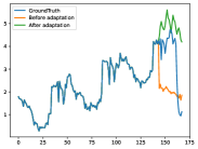
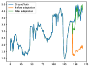
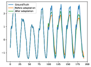
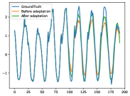
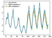
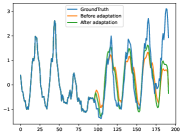
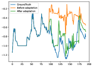
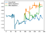
In addition, we conduct case study and visualize our proposed method on various cases across different datasets and models, as presented in Figure 6(h).

Specifically, we plot the figures on these combinations: Illness (timestep 120 & 160, variate 7) on Crossformer, Traffic (timestep 200 & 550, variate 862) on FEDformer, Electricity (timestep 1500 & 3000, variate 321) on Autoformer, and ETTh1 (timestep 250 & 650, variate 7) on Informer, corresponding to Figure 6(h) (a)-(h). The visualization vividly illustrate the effectiveness of our approach in improving forecasting performance.

Figure 5. Case study and visualization of our proposed methods on various cases across different datasets and models, where BLUE lines represent ground-truth, ORANGE lines represent original forecasting results, and GREEN lines represent the forecasts after employing our approach. Besides, $ts120$ denotes this case is sampled at timestep-120 in the test set, and so on.

(a) Illness-ts120

(b) Illness-ts160

(c) Traffic-ts200

(d) Traffic-ts550

(e) Electricity-ts1500

(f) Electricity-ts3000

(g) ETTh1-ts250

(h) ETTh1-ts650

Appendix G Adaptation on Prediction Layer versus Entire Model

All our experiments are performed on solely adapting the prediction layer, as analyzed before, while keeping the crucial parameters of bottom feature extractor layers unchanged. Nevertheless, it is imperative to conduct comparative experiments to validate this persepective. Specifically, we compare the results achieved by solely adapting the prediction layer against adapting the entire model. The experimental results are presented in Table 6.

Based on the comparative results and analysis, it clarifies that solely adapting prediction layer consistently yields superior performance. Additionally, solely adapting prediction layer offers several advantages, including faster adaptation speed, preserving the important bottom parameters unchanged, and reducing the risk of over-fitting on the model.

Table 6. Performance comparison between adaptation on prediction layer versus adaptation on entire model. ”/” indicates original forecasts without SOLID. SOLID-P denotes method SOLID is solely employed on Prediction layer, while SOLID-E denotes SOLID on the Entire model. And ”pl96” or ”pl192” means that the prediction length is 96 or 192 respectively.

Dataset		ETTh1+pl96		ETTh1+pl192		Traffic+pl96		Traffic+pl192		Illness+pl24		Illness+pl36
Metric		MSE	MAE	MSE	MAE	MSE	MAE	MSE	MAE	MSE	MAE	MSE	MAE
Informer	/	0.948	0.774	1.009	0.786	0.731	0.406	0.739	0.414	5.096	1.533	5.078	1.535
	+SOLID-P	0.684	0.586	0.759	0.624	0.628	0.393	0.653	0.413	2.874	1.150	3.299	1.243
	+SOLID-E	0.817	0.656	0.859	0.667	0.692	0.403	0.703	0.417	2.991	1.208	3.476	1.272
Autoformer	/	0.440	0.444	0.487	0.472	0.621	0.391	0.713	0.417	3.314	1.245	2.733	1.078
	+SOLID-P	0.430	0.442	0.480	0.470	0.565	0.376	0.599	0.379	2.737	1.118	2.540	1.015
	+SOLID-E	0.436	0.443	0.482	0.470	0.597	0.385	0.605	0.403	2.891	1.150	2.655	1.068
FEDformer	/	0.375	0.414	0.427	0.448	0.574	0.356	0.612	0.379	3.241	1.252	2.576	1.048
	+SOLID-P	0.370	0.410	0.420	0.443	0.513	0.344	0.549	0.361	2.707	1.123	2.365	0.990
	+SOLID-E	0.373	0.413	0.425	0.447	0.539	0.348	0.562	0.366	2.874	1.201	2.533	1.040
ETSformer	/	0.495	0.480	0.543	0.505	0.599	0.386	0.611	0.391	2.397	0.993	2.504	0.970
	+SOLID-P	0.491	0.478	0.538	0.503	0.487	0.354	0.492	0.354	2.262	0.955	2.301	0.934
	+SOLID-E	0.492	0.479	0.541	0.504	0.517	0.368	0.523	0.374	2.353	0.986	2.339	0.965
Crossformer	/	0.411	0.432	0.419	0.444	0.521	0.297	0.523	0.298	3.329	1.275	3.392	1.185
	+SOLID-P	0.382	0.415	0.396	0.422	0.473	0.267	0.475	0.270	2.397	1.052	2.527	1.042
	+SOLID-E	0.401	0.427	0.399	0.428	0.493	0.273	0.497	0.275	2.653	1.074	2.523	1.017

References

- (1)
- dis (2015) 2015. Learning theory and algorithms for forecasting non-stationary time series. Advances in Neural Information Processing Systems 2015-January (2015), 541–549.
- Ahmadi et al. (2019) Mohsen Ahmadi, Saeid Ghoushchi, Rahim Taghizadeh, and Abbas Sharifi. 2019. Presentation of a new hybrid approach for forecasting economic growth using artificial intelligence approaches. Neural Computing and Applications 31 (12 2019), 8661–8680. https://doi.org/10.1007/s00521-019-04417-0
- Angryk et al. (2020) Rafal Angryk, Petrus Martens, Berkay Aydin, Dustin Kempton, Sushant Mahajan, Sunitha Basodi, Azim Ahmadzadeh, Xumin Cai, Soukaina Filali Boubrahimi, Shah Muhammad Hamdi, Michael Schuh, and Manolis Georgoulis. 2020. Multivariate time series dataset for space weather data analytics. Scientific Data 7 (07 2020), 227. https://doi.org/10.1038/s41597-020-0548-x
- Arik et al. (2022) Sercan O. Arik, Nathanael C. Yoder, and Tomas Pfister. 2022. Self-Adaptive Forecasting for Improved Deep Learning on Non-Stationary Time-Series. arXiv:2202.02403 [cs.LG]
- Bach (2023) Francis Bach. 2023. Learning theory from first principles. (2023).
- Deb et al. (2017) Chirag Deb, Fan Zhang, Junjing Yang, Siew Eang Lee, and Kwok Wei Shah. 2017. A review on time series forecasting techniques for building energy consumption. Renewable and Sustainable Energy Reviews 74 (2017), 902–924. https://doi.org/10.1016/j.rser.2017.02.085
- Demirel et al. (2012) Funda Demirel, Selim Zaim, Ahmet Caliskan, and Pinar Gokcin Ozuyar. 2012. Forecasting natural gas consumption in Istanbul using neural networks and multivariate time series methods. Turkish Journal of Electrical Engineering and Computer Sciences 20 (01 2012), 695–711. https://doi.org/10.3906/elk-1101-1029
- Devlin et al. (2019) Jacob Devlin, Ming-Wei Chang, Kenton Lee, and Kristina Toutanova. 2019. BERT: Pre-training of Deep Bidirectional Transformers for Language Understanding. In Proceedings of the 2019 Conference of the North American Chapter of the Association for Computational Linguistics: Human Language Technologies, Volume 1 (Long and Short Papers). Association for Computational Linguistics, Minneapolis, Minnesota, 4171–4186. https://doi.org/10.18653/v1/N19-1423
- Dosovitskiy et al. (2021) Alexey Dosovitskiy, Lucas Beyer, Alexander Kolesnikov, Dirk Weissenborn, Xiaohua Zhai, Thomas Unterthiner, Mostafa Dehghani, Matthias Minderer, Georg Heigold, Sylvain Gelly, Jakob Uszkoreit, and Neil Houlsby. 2021. An Image is Worth 16x16 Words: Transformers for Image Recognition at Scale. In International Conference on Learning Representations. https://openreview.net/forum?id=YicbFdNTTy
- Du et al. (2021) Yuntao Du, Jindong Wang, Wenjie Feng, Sinno Pan, Tao Qin, Renjun Xu, and Chongjun Wang. 2021. AdaRNN: Adaptive Learning and Forecasting of Time Series. In Proceedings of the 30th ACM International Conference on Information & Knowledge Management (Virtual Event, Queensland, Australia) (CIKM ’21). Association for Computing Machinery, New York, NY, USA, 402–411. https://doi.org/10.1145/3459637.3482315
- Fan et al. (2023) Wei Fan, Pengyang Wang, Dongkun Wang, Dongjie Wang, Yuanchun Zhou, and Yanjie Fu. 2023. Dish-TS: a general paradigm for alleviating distribution shift in time series forecasting. In Proceedings of the AAAI Conference on Artificial Intelligence, Vol. 37. 7522–7529.
- Hu et al. (2015) Yan Hu, Qimin Peng, Xiaohui Hu, and Rong Yang. 2015. Web Service Recommendation Based on Time Series Forecasting and Collaborative Filtering. In 2015 IEEE International Conference on Web Services. 233–240. https://doi.org/10.1109/ICWS.2015.40
- Karevan and Suykens (2020) Zahra Karevan and Johan A.K. Suykens. 2020. Transductive LSTM for time-series prediction: An application to weather forecasting. Neural Networks 125 (2020), 1–9. https://doi.org/10.1016/j.neunet.2019.12.030
- Kim et al. (2022) Taesung Kim, Jinhee Kim, Yunwon Tae, Cheonbok Park, Jang-Ho Choi, and Jaegul Choo. 2022. Reversible Instance Normalization for Accurate Time-Series Forecasting against Distribution Shift. In International Conference on Learning Representations. https://openreview.net/forum?id=cGDAkQo1C0p
- Kulinski et al. (2020) Sean Kulinski, Saurabh Bagchi, and David I Inouye. 2020. Feature shift detection: Localizing which features have shifted via conditional distribution tests. Advances in neural information processing systems 33 (2020), 19523–19533.
- Lai et al. (2018) Guokun Lai, Wei-Cheng Chang, Yiming Yang, and Hanxiao Liu. 2018. Modeling long-and short-term temporal patterns with deep neural networks. In The 41st international ACM SIGIR conference on research & development in information retrieval. 95–104.
- Lipton et al. (2018) Zachary Lipton, Yu-Xiang Wang, and Alexander Smola. 2018. Detecting and correcting for label shift with black box predictors. In International conference on machine learning. PMLR, 3122–3130.
- Passalis et al. (2019) Nikolaos Passalis, Anastasios Tefas, Juho Kanniainen, Moncef Gabbouj, and Alexandros Iosifidis. 2019. Deep adaptive input normalization for time series forecasting. IEEE transactions on neural networks and learning systems 31, 9 (2019), 3760–3765.
- Patton (2013) Andrew Patton. 2013. Chapter 16 - Copula Methods for Forecasting Multivariate Time Series. In Handbook of Economic Forecasting, Graham Elliott and Allan Timmermann (Eds.). Handbook of Economic Forecasting, Vol. 2. Elsevier, 899–960. https://doi.org/10.1016/B978-0-444-62731-5.00016-6
- Pearl (2009) Judea Pearl. 2009. Causality. Cambridge university press.
- Rabanser et al. (2019) Stephan Rabanser, Stephan Günnemann, and Zachary Lipton. 2019. Failing loudly: An empirical study of methods for detecting dataset shift. Advances in Neural Information Processing Systems 32 (2019).
- Singh et al. (2020a) Vijendra Pratap Singh, Manish Kumar Pandey, Pangambam Sendash Singh, and Subbiah Karthikeyan. 2020a. An Econometric Time Series Forecasting Framework for Web Services Recommendation. Procedia Computer Science 167 (2020), 1615–1625. https://doi.org/10.1016/j.procs.2020.03.372 International Conference on Computational Intelligence and Data Science.
- Singh et al. (2020b) Vijendra Pratap Singh, Manish Kumar Pandey, Pangambam Sendash Singh, and Subbiah Karthikeyan. 2020b. Neural Net Time Series Forecasting Framework for Time-Aware Web Services Recommendation. Procedia Computer Science 171 (2020), 1313–1322. https://doi.org/10.1016/j.procs.2020.04.140 Third International Conference on Computing and Network Communications (CoCoNet’19).
- Smyl (2019) Slawek Smyl. 2019. A hybrid method of exponential smoothing and recurrent neural networks for time series forecasting. International Journal of Forecasting 36 (07 2019). https://doi.org/10.1016/j.ijforecast.2019.03.017
- Vaswani et al. (2017) Ashish Vaswani, Noam Shazeer, Niki Parmar, Jakob Uszkoreit, Llion Jones, Aidan N Gomez, Łukasz Kaiser, and Illia Polosukhin. 2017. Attention is all you need. Advances in neural information processing systems 30 (2017).
- Woo et al. (2022) Gerald Woo, Chenghao Liu, Doyen Sahoo, Akshat Kumar, and Steven C. H. Hoi. 2022. ETSformer: Exponential Smoothing Transformers for Time-series Forecasting. CoRR abs/2202.01381 (2022). arXiv:2202.01381 https://arxiv.org/abs/2202.01381
- Wu et al. (2023) Haixu Wu, Tengge Hu, Yong Liu, Hang Zhou, Jianmin Wang, and Mingsheng Long. 2023. TimesNet: Temporal 2D-Variation Modeling for General Time Series Analysis. In The Eleventh International Conference on Learning Representations. https://openreview.net/forum?id=ju_Uqw384Oq
- Wu et al. (2021) Haixu Wu, Jiehui Xu, Jianmin Wang, and Mingsheng Long. 2021. Autoformer: Decomposition transformers with auto-correlation for long-term series forecasting. Advances in Neural Information Processing Systems 34 (2021), 22419–22430.
- Zhang and Yan (2023) Yunhao Zhang and Junchi Yan. 2023. Crossformer: Transformer Utilizing Cross-Dimension Dependency for Multivariate Time Series Forecasting. In The Eleventh International Conference on Learning Representations. https://openreview.net/forum?id=vSVLM2j9eie
- Zhou et al. (2021) Haoyi Zhou, Shanghang Zhang, Jieqi Peng, Shuai Zhang, Jianxin Li, Hui Xiong, and Wancai Zhang. 2021. Informer: Beyond efficient transformer for long sequence time-series forecasting. In Proceedings of the AAAI conference on artificial intelligence, Vol. 35. 11106–11115.
- Zhou et al. (2022) Tian Zhou, Ziqing Ma, Qingsong Wen, Xue Wang, Liang Sun, and Rong Jin. 2022. Fedformer: Frequency enhanced decomposed transformer for long-term series forecasting. In International Conference on Machine Learning. PMLR, 27268–27286.