Optimal bounds for the Dunkl kernel in the dihedral case

Abstract.

We establish sharp upper and lower estimates of the Dunkl kernel in the case of dihedral groups.

The heat kernel plays a central role in several branches of mathematics, e.g. in (harmonic) analysis and PDE, in Riemannian (and sub-Riemannian) geometry or in probability theory. In many applications it is desired to know sharp upper and lower estimates in the largest possible space-time regime, see e.g. [7] for a comprehensive presentation. For Riemannian symmetric spaces of non-compact type, the global behavior of the heat kernel was determined in [2] and [3]. In the present paper we are interested in the heat kernel arising in the rational Dunkl theory, which generalizes spherical Fourier analysis on Riemannian symmetric spaces of Euclidean type. In this theory we deal with a finite root system $R$ in a Euclidean space $\mathfrak{a}$. The heat kernel is the fundamental solution of the differential-difference equation

$$\partial_{t}h(t;x,y)=\Delta_{x}h(t;x,y)+\sum_{\alpha\in R^{+}}\kappa(\alpha)\biggl{(}2\frac{\langle{\alpha},{\nabla_{x}h(t;x,y)}\rangle}{\langle{\alpha},{x}\rangle}+|\alpha|^{2}\frac{h(t;s_{\alpha}.x,y)-h(t;x,y)}{\langle{\alpha},{x}\rangle^{2}}\bigg{)}$$

where $\Delta$ denotes the Laplacian on the underlying Euclidean space, $R_{+}$ the collection of positive roots, $\kappa$ the multiplicity function and $s_{\alpha}$ the orthogonal reflection with respect to $\alpha^{\perp}$. The one dimensional case was carefully investigated in [1]. The general case has been recently studied in [5] where the authors obtained the following estimates: there is an explicit rational function $Q(t;x,y)$ and there are constants $C_{1},C_{2}>0$ and $c_{1}>c_{2}>0$ such that

$$C_{1}Q(t;x,y)g^{-c_{1}\frac{d(x,y)^{2}}{t}}\leqslant h(t;x,y)\leqslant C_{2}Q(t;x,y)e^{-c_{2}\frac{d(x,y)^{2}}{t}}$$ (0.1)

where

$$d(x,y)=\min\big{\{}\lvert{x-w.y}\rvert:w\in W\big{\}}$$

denotes the orbital distance under the Weyl group action.

However, since the constants $c_{1}$ and $c_{2}$ are different, the estimates (0.1) are not optimal. Let us recall the expression

$$h(t;x,y)=\frac{1}{c_{k}(2t)^{\gamma+\frac{N}{2}}}\,\exp\bigg{\{}-\frac{|x|^{2}+|y|^{2}}{4t}\bigg{\}}\,E\bigg{(}\frac{x}{\sqrt{2t}},\frac{y}{\sqrt{2t}}\bigg{)}$$

of the heat kernel in terms of the Dunkl kernel $E$, see [8]. The latter is an eigenfunction of all Dunkl operators, which are first order differential-difference operators. In this paper we establish optimal estimates of $E$ (which imply optimal estimates of $h_{t}$) in the dihedral case $I_{n}$.

Our paper is organized as follows. The main result is stated in Theorem 12. Its proof is carried out in Section 3. The overall strategy is explained in Section 2 and the basic notation recalled in Section 1.

Statement

This work started as a joint project with J. Dziubański which aimed at understanding the behavior of the heat kernel in the rational Dunkl setting beyond the one dimensional case considered in [1]. In 2017 we obtained an upper bound of the Dunkl kernel for $A_{2}$ which was announced by J. Dziubański during his talk at the conference “Analysis and Applications” organized in honor of E.M. Stein in September 2017 in Wrocław (https://math.uni.wroc.pl/analysis2017). Later on, J. Dziubański and A. Hejna followed another approach and obtained sharp upper and lower estimates for the heat kernel which, although not optimal, were sufficient for their needs (see [5]). Meanwhile we realized that our upper bound for $A_{2}$ was also a lower bound. At the same time we obtained similar results for $B_{2}$. Finally in June 2023, P. Graczyk and P. Sawyer informed us that they were obtaining an upper and lower bound for $A_{2}$ by a completely different method, relying on a positive integral formula $($see [6]$)$.

1. Elements of rational Dunkl theory

In this section we introduce the necessary notation to define Dunkl kernels. For more details we refer to the pioneer paper [4], see also the surveys [9, 10].

Let $R$ be a reduced (not necessarily crystallographic) finite root system in a $r$-dimensional Euclidean space $\mathfrak{a}$, that is, for each $\alpha\in R$, $s_{\alpha}(R)=R$ and $R\cap\mathbb{R}\alpha=\{-\alpha,\alpha\}$, where

$$s_{\alpha}(x)=x-\langle{x},{\alpha^{\vee}}\rangle\alpha$$

and

$$\alpha^{\vee}=\frac{2}{\langle{\alpha},{\alpha}\rangle}\alpha.$$

We fix a basis $\{\alpha_{1},\alpha_{2},\ldots,\alpha_{r}\}$ of simple roots in $R$. The corresponding subset of positive roots in $R$ will be denoted by $R^{+}$. Let $W$ be the finite reflection group generated by $\{s_{\alpha}:\alpha\in R^{+}\}$. The fundamental domain for the action of $W$ on $\mathfrak{a}$ is the sector

$$\mathfrak{a}_{+}=\big{\{}x\in\mathfrak{a}:\langle{\alpha},{x}\rangle>0\text{ for all }\alpha\in R^{+}\big{\}}.$$

Let $\kappa:R\rightarrow(0,\infty)$ be a positive multiplicity function on $R$, that is $\kappa$ is invariant under the action of $W$ on $R$. The Dunkl operators, resp. the Dunkl kernel $E(x,y)$ are $\kappa$-deformations of directional derivatives, resp. of the exponential function $e^{\langle{x},{y}\rangle}$. More precisely, the Dunkl operators are defined by

$$T_{\xi}f(x)=\langle{\xi},{\nabla f(x)}\rangle+\sum_{\alpha\in R^{+}}\kappa(\alpha)\,\langle{\alpha},{\xi}\rangle\,\frac{f(x)-f(s_{\alpha}x)}{\langle{\alpha},{x}\rangle}\quad\text{for every \,}\xi\in\mathfrak{a},$$

they commute pairwise and, for every $y\in\mathfrak{a}$, $E(\cdot,y)$ is the unique smooth solution to

$$\begin{cases}\,T_{\xi}f=\langle{\xi},{y}\rangle f\quad\text{for all }\xi\in\mathfrak{a},\\ \,f(0)=1.\end{cases}$$ (1.1)

The Dunl kernel $E$ extends to a holomorphic function on $\mathfrak{a}_{\mathbb{C}}\times\mathfrak{a}_{\mathbb{C}}$, which satisfies

• $E(x,y)=E(y,x)$;

• $E(\lambda x,y)=E(x,\lambda y)$, for all $\lambda\in\mathbb{C}$;

• $E(w.x,w.y)=E(x,y)$, for all $w\in W$;

• $\overline{E(x,y)}=E(\overline{x},\overline{y})$.

Moreover $E(x,y)>0$ when $x,y\in\mathfrak{a}$. Our aim is to obtain sharp upper and lower estimates for $E$ on $\mathfrak{a}\times\mathfrak{a}$.

2. The strategy

In order to estimate the Dunkl kernel $E$, our strategy consists in using the differential-difference equations satisfied by $E$ and in constructing appropriate barrier functions. As an illustration, let us first consider the one dimensional case.

2.1. Example : the one dimensional case

Let us recall that $E:\mathbb{R}\times\mathbb{R}\rightarrow\mathbb{C}$ satisfies

$$\left\{\begin{aligned} &\frac{\partial}{\partial x}E(x,y)+\frac{\kappa}{x}\big{\{}E(x,y)-E(x,-y)\big{\}}=yE(x,y)\\ &\frac{\partial}{\partial x}E(x,-y)+\frac{\kappa}{x}\big{\{}E(x,-y)-E(x,y)\big{\}}=-yE(x,-y)\end{aligned}\quad\text{ for all }x,y\geqslant 0,\right.$$

with the initial condition $E(x,y)=1$ whenever $xy=0$. Given $c>0$, we define

$$\tilde{E}(x,y) =(1+cxy)^{\kappa}e^{-xy}E(x,y),$$

$$\tilde{E}(x,-y) =(1+cxy)^{\kappa+1}e^{-xy}E(x,-y),$$

for all $x,y\geq 0$. Then

$$\frac{\partial}{\partial x}\tilde{E}(x,y) =\frac{\kappa}{x(1+cxy)}\{\tilde{E}(x,-y)-\tilde{E}(x,y)\},$$ (2.1)

$$\frac{\partial}{\partial x}\tilde{E}(x,-y) =\frac{\kappa(1+cxy)}{x}\{\tilde{E}(x,y)-\tilde{E}(x,-y)\}+\frac{(2\kappa+1)c+(\kappa c-2)cxy-2}{1+cxy}y\tilde{E}(x,-y).$$ (2.2)

Let us fix $y>0$.

Upper bound: Let $c$ be small, say $0<c<\frac{2}{2\kappa+1}$. Hence,

$$\tfrac{(2\kappa+1)c+(\kappa c-2)cxy-2}{1+cxy}<0.$$ (2.3)

We claim that the function

$$M(x)=\max\big{\{}\tilde{E}(x,y),\tilde{E}(x,-y)\big{\}}$$

is a decreasing function on $[0,\infty)$. Indeed, on any interval $[a,b]$ where $\tilde{E}(x,y)\geqslant\tilde{E}(x,-y)$, by (2.1) we have $\tfrac{\partial}{\partial x}\tilde{E}(x,y)\leqslant 0$. Hence

$$\tilde{E}(x,-y)\leqslant\tilde{E}(x,y)\leqslant\tilde{E}(a,y)=M(a).$$

Similarly, on any interval $[a,b]$ where $\tilde{E}(x,y)\leqslant\tilde{E}(x,-y)$, by (2.3) and (2.2) we have $\tfrac{\partial}{\partial x}\tilde{E}(x,-y)\leqslant 0$. Hence

$$\tilde{E}(x,y)\leqslant\tilde{E}(x,-y)\leqslant\tilde{E}(a,-y)=M(a).$$

In both cases, $M(x)\leqslant M(a)$ on $[a,b]$. Therefore, $M(x)\leqslant M(0)=1$ on $[0,\infty)$.

Lower bound: We argue similarly, assuming that $c$ is large, say $c>\tfrac{2}{\kappa}$. Hence,

$$\tfrac{(2\kappa+1)c+(\kappa c-2)cxy-2}{1+cxy}>0.$$ (2.4)

The function

$$m(x)=\min\big{\{}\tilde{E}(x,y),\tilde{E}(x,-y)\big{\}}$$

is an increasing function on $[0,\infty)$. Indeed, on any interval $[a,b]$ where $\tilde{E}(x,y)\leqslant\tilde{E}(x,-y)$, by (2.1) we have $\tfrac{\partial}{\partial x}\tilde{E}(x,y)\geqslant 0$. Hence

$$\tilde{E}(x,-y)\geqslant\tilde{E}(x,y)\geqslant\tilde{E}(a,y)=m(a).$$

Similarly, on any interval $[a,b]$ where $\tilde{E}(x,y)\geqslant\tilde{E}(x,-y)$, by (2.4) and (2.2) we have $\tfrac{\partial}{\partial x}\hskip 0.85358pt\tilde{E}(x,-y)\geqslant 0$. Therefore,

$$\tilde{E}(x,y)\geqslant\tilde{E}(x,-y)\geqslant\tilde{E}(a,-y)=m(a).$$

In both cases, $m(x)\geqslant m(a)$ on $[a,b]$. Hence $m(x)\geqslant m(0)=1$ on $[0,\infty)$.

In conclusion we obtain the following global bound :

$$E(x,y)\approx\frac{e^{xy}}{(1+|xy|)^{\kappa}}\times\begin{cases}\,1&\text{if $xy\geqslant 0$,}\\ \,(1+|xy|)^{-1}&\text{if $xy\leqslant 0$.}\\ \end{cases}$$

2.2. General root system

We set

$$\tilde{E}_{w}(x,y)=E(x,w.y)e^{-\langle x,y\rangle}Q_{w}(x,y)\prod_{\alpha\in R^{+}}\big{(}1+c\langle{\alpha},{x}\rangle\langle{\alpha},{y}\rangle\big{)}^{\kappa(\alpha)}\quad\text{for every \,}w\in W\text{ and }x,y\in\overline{\mathfrak{a}_{+}},$$

where $c$ is a positive constant and the $Q_{w}$’s are barrier functions, to be determined, which are positive rational functions on $\overline{\mathfrak{a}_{+}}\times\overline{\mathfrak{a}_{+}}$. Taking $\xi=x$ in (1.1), we get

$$\langle{x},{\nabla_{x}}\rangle E(x,w.y)+\sum_{\alpha\in R^{+}}\kappa(\alpha)\big{\{}E(x,w.y)-E(r_{\alpha}.x,w.y)\big{\}}=\langle{x},{w.y}\rangle E(x,w.y),$$

thus

$$\frac{\langle{x},{\nabla_{x}}\rangle\tilde{E}_{w}(x,y)}{\tilde{E}_{w}(x,y)} =\langle{x},{w.y}\rangle-\langle{x},{y}\rangle+\frac{\langle{x},{\nabla_{x}}\rangle Q_{w}(x,y)}{Q_{w}(x,y)}+\sum_{\alpha\in R^{+}}\kappa(\alpha)\frac{c\langle{\alpha},{x}\rangle\langle{\alpha},{y}\rangle}{1+c\langle{\alpha},{x}\rangle\langle{\alpha},{y}\rangle}$$

$$\phantom{=}-\sum_{\alpha\in R^{+}}\kappa(\alpha)\bigg{\{}1-\frac{Q_{w}(x,y)}{Q_{s_{\alpha}w}(x,y)}\frac{\tilde{E}_{s_{\alpha}w}(x,y)}{\tilde{E}_{w}(x,y)}\bigg{\}}.$$

Hence

$$\langle{x},{\nabla_{x}}\rangle\tilde{E}_{w}(x,y) =-\sum_{\alpha\in R^{+}}\kappa(\alpha)\frac{Q_{w}(x,y)}{Q_{s_{\alpha}w}(x,y)}\big{\{}\tilde{E}_{w}(x,y)-\tilde{E}_{s_{\alpha}w}(x,y)\big{\}}$$

$$\phantom{=}-\Lambda_{w}(x,y)\tilde{E}_{w}(x,y),$$

where

$$\Lambda_{w}(x,y) =\langle{x},{y-w.y}\rangle-\frac{\langle{x},{\nabla_{x}}\rangle Q_{w}(x,y)}{Q_{w}(x,y)}$$ (2.5)

$$\phantom{=}+\sum_{\alpha\in R^{+}}\kappa(\alpha)\bigg{\{}\frac{1}{1+c\langle{\alpha},{x}\rangle\langle{\alpha},{y}\rangle}-\frac{Q_{w}(x,y)}{Q_{s_{\alpha}w}(x,y)}\bigg{\}}.$$

Our aim is to find positive rational functions $Q_{w}(x,y)$ and constants $c_{+}\geqslant c_{-}>0$ such that

$$\Lambda_{w}(x,y)\geqslant 0,\quad\text{ for all }x,y\in\overline{\mathfrak{a}_{+}}\text{ and }c\in(0,c_{-}),$$ (2.6)

and

$$\Lambda_{w}(x,y)\leqslant 0,\quad\text{ for all }x,y\in\mathfrak{a}_{+}\text{ and }c\in(c_{+},\infty).$$ (2.7)

Once (2.6) and (2.7) are achieved, we deduce as in the one dimensional case that

• $M(t)=\max_{w\in W}\tilde{E}_{w}(tx,y)$ is a decreasing function of $t\in[0,\infty)$ when $c\in(0,c_{-})$,

• $m(t)=\min_{w\in W}\tilde{E}_{w}(tx,y)$ is an increasing function of $t\in[0,\infty)$ when $c\in(c_{+},\infty)$,

and we conclude that

$$M(1)\leqslant M(0)=1=m(0)\leqslant m(1)\,.$$

Currently we are able to complete this program for dihedral root systems, which are all (non necessarily crystallographic) $2$-dimensional irreducible root systems. For general root systems we intend to return to the problem in the future.

3. The Dunkl kernel for dihedral root systems

In this section we establish optimal bounds for the Dunkl kernel in the dihedral case, which includes in particular the root system $A_{2}$ considered in [6].

3.1. Dihedral root systems

Let us start by introducing the necessary notation. Let $I_{n}$, $n\geqslant 3$, be the root system in $\mathfrak{a}=\mathbb{R}^{2}$ consisting of vectors

$$\Big{\{}\pm\big{(}\cos\tfrac{\pi j}{n},\sin\tfrac{\pi j}{n}\big{)}:j\in\{0,1,\ldots,n-1\}\Big{\}}.$$

Let us observe that the ends of the vectors in $I_{n}$ represent the vertices of the regular $(2n)$-gon in $\mathbb{R}^{2}$. We set

$$\alpha_{j}=\big{(}\cos\tfrac{\pi j}{n},\sin\tfrac{\pi j}{n}\big{)},\quad\text{ for }j\in\{0,1,\ldots,n-1\}.$$

Then $\{\alpha_{0},\alpha_{1},\ldots,\alpha_{n-1}\}$ is the set of positive roots in $I_{n}$. The positive Weyl chamber is

$$\mathfrak{a}_{+}=\big{\{}x\in\mathbb{R}^{2}:\langle{\alpha_{0}},{x}\rangle>0\text{ and }\langle{\alpha_{n-1}},{x}\rangle>0\big{\}}.$$

The corresponding Weyl (or Coxeter) group has presentation

$$W=\langle r,s:r^{n}=\operatorname{Id}=s^{2},srs=r^{-1}\rangle.$$

In fact, the group $W$ is the dihedral group which consists of $n$ rotations

$$r_{j}=r^{j}=\begin{pmatrix}\cos\frac{2\pi j}{n}&-\sin\frac{2\pi j}{n}\\ \sin\frac{2\pi j}{n}&\cos\frac{2\pi j}{n}\end{pmatrix},\quad j\in\mathbb{Z}/n\mathbb{Z},$$

and $n$ reflections (or symmetries)

$$s_{j}=sr^{j}=\begin{pmatrix}-\cos\frac{2\pi j}{n}&\sin\frac{2\pi j}{n}\\ \sin\frac{2\pi j}{n}&\cos\frac{2\pi j}{n}\end{pmatrix},\quad j\in\mathbb{Z}/n\mathbb{Z}.$$

If $n$ is odd then all roots are in the same $W$-orbit while, if $n$ is even there are two $W$-orbits: $W\!.\alpha_{0}$ and $W\!.\alpha_{1}$. Thus, if $n$ is odd, we set $\kappa>0$ to be the joint multiplicity of all roots while, if $n$ is even, we let $\kappa_{0}>0$, respectively $\kappa_{1}>0$, to be the multiplicity of the roots in $W\!.\alpha_{0}$, respectively in $W\!.\alpha_{1}$. Set

$$\kappa_{\hskip 0.85358pt\min}=\begin{cases}\kappa&\text{if $n$ is odd,}\\ \min\{\kappa_{0},\kappa_{1}\}&\text{if $n$ is even,}\end{cases}\quad\text{and}\quad\kappa_{\hskip 0.85358pt\max}=\begin{cases}\kappa&\text{if $n$ is odd,}\\ \max\{\kappa_{0},\kappa_{1}\}&\text{if $n$ is even.}\\ \end{cases}$$

See Figure 1 for a picture of $I_{5}$.

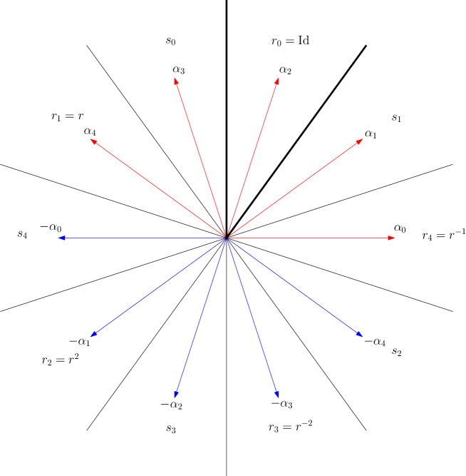
Figure 1. The case $n=5$

Given $x,y\in\smash{\overline{\mathfrak{a}_{+}}}$ and $j\in\mathbb{Z}/n\mathbb{Z}$, we define

$$\rho_{j} =\langle{x},{y-r_{j}.y}\rangle,\qquad \sigma_{j} =\langle{x},{y-s_{j}.y}\rangle,$$

$$D_{r_{j}} =1+c\rho_{j}, D_{s_{j}} =1+c\sigma_{j}.$$

Let

$$D_{R} =\prod_{j\in\mathbb{Z}/n\mathbb{Z}}D_{r_{j}},\qquad D_{S} =\prod_{j\in\mathbb{Z}/n\mathbb{Z}}D_{s_{j}},$$

$$\mathfrak{D}_{R} =\sum_{j\in\mathbb{Z}/n\mathbb{Z}}\frac{1}{D_{r_{j}}},\qquad \mathfrak{D}_{S} =\sum_{j\in\mathbb{Z}/n\mathbb{Z}}\frac{1}{D_{s_{j}}},$$

and

$$\mathfrak{S}=\prod_{j\in\mathbb{Z}/n\mathbb{Z}}\sigma_{j}.$$

Let us observe that both $\rho_{j}$ and $\sigma_{j}$ are non-negative for every $j\in\mathbb{Z}/n\mathbb{Z}$. Moreover, $\rho_{0}=0$ and $D_{r_{0}}=1$ are trivial. The following two lemmas allows us to compare the $\rho_{j}$’s and $\sigma_{j}$’s

Lemma 1.

The following properties hold, for all $x,y\in\smash{\overline{\mathfrak{a}_{+}}}$:

$$\left\{\begin{aligned} \sigma_{0}&=2\langle{\alpha_{0}},{x}\rangle\langle{\alpha_{0}},{y}\rangle,\\ \sigma_{1}&=2\langle{\alpha_{n-1}},{x}\rangle\langle{\alpha_{n-1}},{y}\rangle,\\ \sigma_{j}&\approx\langle{x},{y}\rangle,\quad\text{for all }j\in\{2,\ldots,n-1\},\end{aligned}\right.\quad\text{and}\quad\left\{\begin{aligned} \rho_{1}&=2\big{(}\sin\tfrac{\pi}{n}\big{)}\langle{\tilde{r}.x},{y}\rangle,\\ \rho_{n-1}&=2\big{(}\sin\tfrac{\pi}{n}\big{)}\langle{x},{\tilde{r}.y}\rangle,\\ \rho_{j}&\approx\langle{x},{y}\rangle,\quad\text{for all }j\in\{2,3,\ldots,n-2\},\end{aligned}\right.$$

where $\tilde{r}$ is the rotation about the origin in $\mathbb{R}^{2}$ by the angle $(\frac{\pi}{2}-\frac{\pi}{n})$, that is

$$\tilde{r}=\begin{pmatrix}\sin\frac{\pi}{n}&-\cos\frac{\pi}{n}\\ \cos\frac{\pi}{n}&\sin\frac{\pi}{n}\end{pmatrix}.$$ (3.1)

Proof.

Since for each $j\in\{0,1,\ldots,n-1\}$, $s_{-j}$ is the reflection with respect to $\alpha_{j}^{\perp}$, we get

$$\sigma_{-j}=2\langle{\alpha_{j}},{x}\rangle\langle{\alpha_{j}},{y}\rangle.$$

If $0<j<n-1$, then both $\sigma_{-j}$ and $\langle{x},{y}\rangle$ reach (strictly) positive extrema, as $x$ and $y$ run through the compact set

$$\text{S}(\smash{\overline{\mathfrak{a}_{+}}})=\big{\{}z\in\smash{\overline{\mathfrak{a}_{+}}}:\lvert{z}\rvert=1\big{\}}.$$

Hence, by homogeneity, we deduce that

$$\sigma_{-j}\approx\langle{x},{y}\rangle,\quad\text{ for all }x,y\in\smash{\overline{\mathfrak{a}_{+}}}.$$

Let us now turn to rotations. Notice that

$$\operatorname{Id}-r_{j}=2\big{(}\sin\tfrac{\pi j}{n}\big{)}\begin{pmatrix}\sin\frac{\pi j}{n}&\cos\frac{\pi j}{n}\\ -\cos\frac{\pi j}{n}&\sin\frac{\pi j}{n}\end{pmatrix}$$

where the matrix represents the rotation about the origin in $\mathbb{R}^{2}$ by the angle $(\frac{\pi j}{n}-\frac{\pi}{2})$. We deduce on the one hand that

$$\left\{\begin{aligned} \rho_{1}&=2(\sin\tfrac{\pi}{n})\langle{x},{(\tilde{r})^{-1}.y}\rangle,\\ \rho_{n-1}&=2(\sin\tfrac{\pi}{n})\langle{x},{\tilde{r}.y}\rangle.\end{aligned}\right.$$

On the other hand, for $1<j<n-1$, the image $(\operatorname{Id}-r_{j}).\text{S}(\smash{\overline{\mathfrak{a}_{+}}})$ doesn’t meet $\text{S}(\smash{\overline{\mathfrak{a}_{+}}})$, thus arguing as for reflections we arrive at

$$\rho_{j}\approx\langle{x},{y}\rangle,\quad\text{ for all }x,y\in\smash{\overline{\mathfrak{a}_{+}}}.\qed$$

Lemma 2.

For each $j\in\mathbb{Z}/n\mathbb{Z}\smallsetminus\{0\}$, there is $k\in\mathbb{Z}/n\mathbb{Z}$ such that

$$\rho_{j}\geqslant\sigma_{k},\quad\text{ for all }x,y\in\smash{\overline{\mathfrak{a}_{+}}}.$$

Proof.

Let $j\in\mathbb{Z}/n\mathbb{Z}\smallsetminus\{0\}$. As $r_{-j}\neq\operatorname{Id}$, there exists a positive root $\alpha_{\ell}$ such that $r_{-j}.\alpha_{\ell}$ is negative. Let $k\equiv j-\ell\pmod{n}$, so that $s_{k-j}=s_{-\ell}$ is the reflection with respect to $\alpha_{\ell}^{\perp}$. Then

$$\rho_{j}-\sigma_{k} =\langle{x},{s_{k}.y-r_{j}.y}\rangle$$

$$=\langle{x},{s_{k-j}(r_{j}.y)-r_{j}.y}\rangle$$

$$=-2\underbrace{\langle{\alpha_{\ell}},{x}\rangle}_{\geqslant 0}\underbrace{\langle{\alpha_{\ell}},{r_{j}.y}\rangle}_{\leqslant 0}\geqslant 0.\qed$$

Later we will also need the following lemma.

Lemma 3.

For $m_{1},\ldots,m_{k}\in\mathbb{Z}/n\mathbb{Z}$, we set

$$I(m_{1},\dots,m_{k})=\sum_{\stackrel{{\scriptstyle{j_{1},\ldots,j_{k}\in\mathbb{Z}/n\mathbb{Z}}}}{{{\mathrm{distinct}}}}}e^{\mathrm{i}\frac{2\pi}{n}(m_{1}j_{1}+\ldots+m_{k}j_{k})}.$$ (3.2)

Then

1. $I(m_{1},\dots,m_{k})$ is real valued and symmetric under permutations of $m_{1},\ldots,m_{k}$;

2. $I(m_{1},\dots,m_{k})=\begin{cases}(n-k+1)I(m_{1},\ldots,m_{k-1})&\text{if $m_{k}\equiv 0\pmod{n}$},\\ -\sum_{1\leqslant i<k}I(m_{1},\ldots,m_{i}+m_{k},\ldots,m_{k-1})&\text{if $m_{k}\not\equiv 0\pmod{n}$};\end{cases}$

3. for every $m_{1},\ldots,m_{k}\in\mathbb{Z}/n\mathbb{Z}$, there exists $c\in\mathbb{Z}$ such that

   $$I(m_{1},\ldots,m_{k})=cI(m_{1}+\ldots+m_{k});$$

4. for every $m\in\mathbb{Z}/n\mathbb{Z}$,

   $$I(m)=\begin{cases}n&\text{if $m\equiv 0\pmod{n}$},\\ 0&\text{if $m\not\equiv 0\pmod{n}$}.\end{cases}$$

Proof.

(d) is elementary. (a) is easily deduced from the definition (3.2). Same for the first claim in (b). The second claim in (b) follows from the second claim in (d). Finally (c) is deduced from (b) by induction. ∎

Next, in what follows we need the elementary symmetric polynomials $\mathrm{e}_{j}$ on $n$ variables, namely,

$$\left\{\begin{aligned} \mathrm{e}_{0}(X_{1},\ldots,X_{n})&\equiv 1,\\ \mathrm{e}_{k}(X_{1},\ldots,X_{n})&=\sum_{1\leqslant j_{1}<\ldots<j_{k}\leqslant n}X_{j_{1}}X_{j_{2}}\cdots X_{j_{k}},\quad 1\leqslant k<n\\ \mathrm{e}_{n}(X_{1},\ldots,X_{n})&=X_{1}X_{2}\cdots X_{n}.\end{aligned}\right.$$ (3.3)

A straightforward argument shows that for $k\in\{1,\ldots,n-1\}$,

$$\mathrm{e}_{k}(X_{1},\ldots,X_{n})=\frac{1}{k!}\sum_{\stackrel{{\scriptstyle{1\leq j_{1},\ldots,j_{k}\leq n}}}{{{\text{distinct}}}}}X_{j_{1}}X_{j_{2}}\cdots X_{j_{k}}.$$

Recall that the elementary symmetric polynomials generate the algebra of symmetric polynomials in $n$ variables.

The following lemma allows us to compare symmetric polynomials in $\rho_{j}$’s and $\sigma_{j}$’s.

Lemma 4.

For each $k\in\{0,1,\ldots,n-1\}$,

$$\mathrm{e}_{k}(\rho_{0},\dots,\rho_{n-1})=\mathrm{e}_{k}(\sigma_{0},\dots,\sigma_{n-1})$$

while $\mathrm{e}_{n}(\rho_{0},\dots,\rho_{n-1})=0$ and $\mathrm{e}_{n}(\sigma_{0},\dots,\sigma_{n-1})=\mathfrak{S}$.

Remark 5.

Let us observe that for all $k\in\{0,1,\ldots,n-1\}$, $\mathrm{e}_{k}(\rho_{0},\rho_{1},\dots,\rho_{n-1})=\mathrm{e}_{k}(\rho_{1},\dots,\rho_{n-1})$.

Proof of Lemma 4.

First of all, the result is immediate when $k=0$ or $k=n$. Since

$$\sum_{j\in\mathbb{Z}/n\mathbb{Z}}r_{j}=0,$$

we deduce that $\mathrm{e}_{1}(\rho_{0},\dots,\rho_{n-1})$ and $\mathrm{e}_{1}(\sigma_{0},\dots,\sigma_{n-1})$ are equal to $n\langle{x},{y}\rangle$. Let us turn to the remaining cases where $1<k<n$ and which are more involved. Let us consider the linear operators

$$S=\underbrace{s\otimes\dots\otimes s}_{\text{$k$ factors}}$$

and

$$R=\sum_{\stackrel{{\scriptstyle{j_{1},\dots,j_{k}\in\mathbb{Z}/n\mathbb{Z}}}}{{{\text{distinct}}}}}r_{j_{1}}\otimes\dots\otimes r_{j_{k}}$$

acting on the space $\textrm{S}^{k}(\mathbb{C}^{2})$ of symmetric tensors in $\otimes^{k}\mathbb{C}^{2}$. Notice that $S$ is an involution which commutes with $R$. We claim that

$$R=SR=RS$$ (3.4)

on $\textrm{S}^{k}(\mathbb{C}^{2})$. Let

$$\textrm{S}^{k}(\mathbb{C}^{2})=E_{+1}\oplus E_{-1}$$

be the eigenspace decomposition of $S$. Then $R(E_{\pm 1})\subset E_{\pm 1}$. Since, (3.4) trivially holds true on $E_{+1}$, it is enough to show that $R=0$ on $E_{-1}$.

For the proof, we introduce suitable bases for our computations. For every $0\leqslant\ell\leqslant k$, let us denote by $\tau_{\ell}$ the sum of tensors $v_{1}\!\otimes\dots\otimes v_{k}$ where $v_{1},\dots,v_{k}$ are equal to $v_{+}=(i,1)$ or $v_{-}=(-i,1)$ with $\ell$ occurrences of $v_{+}$ and $(k-\ell)$ of $v_{-}$. Then $\{\tau_{\ell}:0\leqslant\ell\leqslant k\}$ is a basis of $\textrm{S}^{k}(\mathbb{C}^{2})$. Moreover, as $s(v_{\pm})=v_{\mp}$, we have $S(\tau_{\ell})=\tau_{k-\ell}$. Hence $\{\tau_{\ell}+\tau_{k-\ell}:0\leqslant\ell\leqslant k/2\}$ is a basis of $E_{+1}$, and $\{\tau_{\ell}-\tau_{k-\ell}:0\leqslant\ell<k/2\}$ a basis of $E_{-1}$. Moreover, as

$$r_{j}(v_{\pm})=e^{\pm\mathrm{i}\frac{2\pi j}{n}}v_{\pm},$$

for each $j\in\mathbb{Z}/n\mathbb{Z}$, we obtain

$$R\big{(}\tau_{\ell}-\tau_{k-\ell}\big{)} =R(\tau_{\ell})-R(\tau_{k-\ell})$$

$$=(\operatorname{Re}I_{k,\ell})(\tau_{\ell}-\tau_{k-\ell})+\mathrm{i}(\operatorname{Im}I_{k,\ell})(\tau_{\ell}+\tau_{k-\ell})$$

for each $0\leqslant\ell<k/2$ where $I_{k,\hskip 0.85358pt\ell}$ denotes the exponential sum (3.2) with

$$m_{i}=\begin{cases}1&\text{$\ell$ times,}\\ -1&\text{$(k-\ell)$ times.}\\ \end{cases}$$

Notice that $m_{1}+\ldots+m_{k}=2\ell-k\not\equiv 0\pmod{n}$, as $0\leqslant 2\ell<k<n$. By applying (c) and (d) in Lemma 3, we deduce that $I_{k,\ell}=0$.

In summary, $R$ vanishes on $E_{-1}$ and consequently (3.4) holds true. By applying

$$\sum_{\stackrel{{\scriptstyle{j_{1},\ldots,j_{k}\in\mathbb{Z}/n\mathbb{Z}}}}{{{\mathrm{distinct}}}}}r_{j_{1}}\otimes\ldots\otimes r_{j_{k}}=\sum_{\stackrel{{\scriptstyle{j_{1},\ldots,j_{k}\in\mathbb{Z}/n\mathbb{Z}}}}{{{\mathrm{distinct}}}}}s_{j_{1}}\otimes\ldots\otimes s_{j_{k}}.$$

to $y\otimes\ldots\otimes y$ and taking the inner product with $x\otimes\ldots\otimes x$, we obtain

$$\mathrm{e}_{k}\big{(}\langle{x},{r_{0}.y}\rangle,\ldots,\langle{x},{r_{n-1}.y}\rangle\big{)}=\mathrm{e}_{k}\big{(}\langle{x},{s_{0}.y}\rangle,\ldots,\langle{x},{s_{n-1}.y}\rangle\big{)}$$

for every $1<k<n$. Notice that this equality holds true for $k=0$ and $k=1$ too. We conclude that

$$\mathrm{e}_{k}\big{(}\rho_{0},\ldots,\rho_{n-1}\big{)}=\mathrm{e}_{k}\big{(}\sigma_{0},\ldots,\sigma_{n-1}\big{)}$$ (3.5)

for every $0<k<n$, by expressing both sides of (3.5) as the same polynomial in

$$\mathrm{e}_{k^{\prime}}\big{(}\langle{x},{r_{0}.y}\rangle,\ldots,\langle{x},{r_{n-1}.y}\rangle\big{)}=\mathrm{e}_{k^{\prime}}\big{(}\langle{x},{s_{0}.y}\rangle,\ldots,\langle{x},{s_{n-1}.y}\rangle\big{)}$$

with $0\leqslant k^{\prime}\leqslant k$ and the lemma follows. ∎

Corollary 6.

$D_{R}=D_{S}-c^{n}\mathfrak{S}$.

Proof.

On the one hand,

$$D_{R}=\sum_{0\leqslant k<n}c^{k}\mathrm{e}_{k}(\rho_{0},\ldots,\rho_{n-1}),$$

and on the other hand,

$$D_{S}=\sum_{0\leqslant k\leqslant n}c^{k}\mathrm{e}_{k}(\sigma_{0},\ldots,\sigma_{n-1})$$

with $\mathrm{e}_{n}(\sigma_{0},\ldots,\sigma_{n-1})=\mathfrak{S}$. Then Lemma 4 allows us to conclude. ∎

Corollary 7.

$D_{R}\mathfrak{D}_{R}=D_{S}\mathfrak{D}_{S}$.

Proof.

This is obtained by expressing

$$D_{R}\mathfrak{D}_{R}=\sum_{0\leqslant j<n}D_{r_{0}}\dots D_{r_{j-1}}D_{r_{j+1}}\dots D_{r_{n-1}}$$

and

$$D_{S}\mathfrak{D}_{S}=\sum_{0\leqslant j<n}D_{s_{0}}\dots D_{s_{j-1}}D_{s_{j+1}}\dots D_{s_{n-1}}$$

as the same polynomial in terms of

$$\mathrm{e}_{k}(\sigma_{0},\ldots,\sigma_{n-1})=\mathrm{e}_{k}(\rho_{0},\ldots,\rho_{n-1})$$

with $0\leqslant k<n$. ∎

3.2. Sharp estimates

In this section we prove our main result. To do so, we introduce the following barrier functions:

$$Q_{w}=\begin{cases}1&\text{if }w=\operatorname{Id},\\ D_{s_{j}}&\text{if $w=s_{j}$ $(0\leqslant j<n)$},\\ D_{r_{j}}\frac{D_{S}}{D_{R}}&\text{if $w=r_{j}$ $(0<j<n)$}.\\ \end{cases}$$ (3.6)

We follow the overall strategy presented in Section 2.

Recall that $\Lambda_{\operatorname{Id}}\equiv 1$. We are going to determine the sign of $\Lambda_{w}$ ($w\neq\operatorname{Id}$) depending whether $c>0$ is small or large.

$\bullet$ Assume that $w=s_{j}$ with $j\in\mathbb{Z}/n\mathbb{Z}$. In this case (2.5) writes

$$\Lambda_{s_{j}}=\sigma_{j}-\tfrac{c\sigma_{j}}{D_{s_{j}}}-\kappa(\alpha_{j})\bigl{\{}D_{s_{j}}-\tfrac{1}{D_{s_{j}}}\bigr{\}}-\sum_{\stackrel{{\scriptstyle{k\in\mathbb{Z}/n\mathbb{Z}}}}{{{k\neq j}}}}\kappa(\alpha_{k})\Big{\{}\tfrac{D_{s_{j}}}{D_{r_{k-j}}}\tfrac{D_{R}}{D_{S}}-\tfrac{1}{D_{s_{k}}}\Big{\}},$$

hence

$$\Lambda_{s_{j}}\geqslant\sigma_{j}-A_{j}-\kappa_{\hskip 0.85358pt\max}B_{j}\quad\text{and}\quad\Lambda_{s_{j}}\leqslant\sigma_{j}-\kappa_{\hskip 0.85358pt\min}B_{j},$$

where

$$A_{j}=\tfrac{c\sigma_{j}}{D_{s_{j}}}\quad\text{and}\quad B_{j}=D_{s_{j}}-\tfrac{1}{D_{s_{j}}}+\sum_{\stackrel{{\scriptstyle{k\in\mathbb{Z}/n\mathbb{Z}}}}{{{k\neq j}}}}\Big{\{}\tfrac{D_{s_{j}}}{D_{r_{k-j}}}\tfrac{D_{R}}{D_{S}}-\tfrac{1}{D_{s_{k}}}\Big{\}}.$$

Lemma 8.

We have $B_{j}=c\sigma_{j}C_{j}$ with $2^{1-n}\leqslant C_{j}\leqslant n+1$.

Proof.

We have

$$B_{j} =D_{s_{j}}-\tfrac{1}{D_{s_{j}}}+\tfrac{D_{s_{j}}D_{R}}{D_{S}}\sum_{\stackrel{{\scriptstyle{k\in\mathbb{Z}/n\mathbb{Z}}}}{{{k\neq 0}}}}\tfrac{1}{D_{r_{k}}}-\sum_{\stackrel{{\scriptstyle{k\in\mathbb{Z}/n\mathbb{Z}}}}{{{k\neq j}}}}\tfrac{1}{D_{s_{k}}}$$

$$=\tfrac{D_{s_{j}}}{D_{S}}(D_{S}-D_{R})+\tfrac{D_{s_{j}}D_{R}}{D_{S}}\mathfrak{D}_{R}-\mathfrak{D}_{S}.$$

Using Corollaries 6 and 7, we obtain

$$B_{j}=\tfrac{D_{s_{j}}}{D_{S}}c^{n}\mathfrak{S}+(D_{s_{j}}-1)\mathfrak{D}_{S}=c\sigma_{j}C_{j}$$

where

$$C_{j}=\Big{(}\prod_{\stackrel{{\scriptstyle{k\in\mathbb{Z}/n\mathbb{Z}}}}{{{k\neq j}}}}\tfrac{c\sigma_{k}}{D_{s_{k}}}\Big{)}+\mathfrak{D}_{S}.$$

To conclude, we notice that on the one hand $C_{j}<n+1$. On the other hand, if $c\sigma_{k}\geqslant 1$ for every $k\in\mathbb{Z}/n\mathbb{Z}$, then $C_{j}\geqslant 2^{1-n}$; otherwise, there is $k\in\mathbb{Z}/n\mathbb{Z}$ such that $c\sigma_{k}<1$, thus $C_{j}>\tfrac{1}{D_{s_{k}}}>\tfrac{1}{2}$ which is $\geqslant 2^{1-n}$. ∎

Corollary 9.

We have

1. $\Lambda_{s_{j}}\geqslant 0$, if $0<c\leqslant\tfrac{1}{\kappa_{\hskip 0.85358pt\max}(n+1)+1}$;

2. $\Lambda_{s_{j}}\leqslant 0$, if $c\geqslant\tfrac{2^{n-1}}{\kappa_{\hskip 0.85358pt\min}}$.

Proof.

On the one hand,

$$\Lambda_{s_{j}}\geqslant\sigma_{j}\Big{\{}1-c-c\kappa_{\hskip 0.85358pt\max}(n+1)\Big{\}},$$

which is non-negative provided that $c\leqslant\tfrac{1}{\kappa_{\hskip 0.85358pt\max}(n+1)+1}$. On the other hand,

$$\Lambda_{s_{j}}\leqslant\sigma_{j}\Big{\{}1-c\kappa_{\hskip 0.85358pt\min}2^{1-n}\Big{\}},$$

which is non-positive provided that $c\geqslant\tfrac{2^{n-1}}{\kappa_{\hskip 0.85358pt\min}}$. ∎

$\bullet$ Assume that $w=r_{j}$ with $j\in\mathbb{Z}/n\mathbb{Z}\smallsetminus\{0\}$. In this case, (2.5) writes

$$\Lambda_{r_{j}}=\rho_{j}\sum_{k\in\mathbb{Z}/n\mathbb{Z}}\tfrac{c\sigma_{k}}{D_{s_{k}}}+\sum_{\stackrel{{\scriptstyle{k\in\mathbb{Z}/n\mathbb{Z}\smallsetminus\{0\}}}}{{{k\neq j}}}}\tfrac{c\rho_{k}}{D_{r_{k}}}-\sum_{k\in\mathbb{Z}/n\mathbb{Z}}\kappa(\alpha_{k})\Big{\{}\tfrac{D_{r_{j}}}{D_{s_{k-j}}}\tfrac{D_{S}}{D_{R}}-\tfrac{1}{D_{s_{k}}}\Big{\}}$$

hence

$$\Lambda_{r_{j}}\geqslant\rho_{j}-\tilde{A}_{j}-\kappa_{\hskip 0.85358pt\max}\tilde{B}_{j}\quad\text{and}\quad\Lambda_{r_{j}}\leqslant\rho_{j}-\kappa_{\hskip 0.85358pt\min}\tilde{B}_{j},$$

where

$$\tilde{A}_{j}=\sum_{k\in\mathbb{Z}/n\mathbb{Z}}\tfrac{c\sigma_{k}}{D_{s_{k}}}\sum_{\stackrel{{\scriptstyle{k\in\mathbb{Z}/n\mathbb{Z}\smallsetminus\{0\}}}}{{{k\neq j}}}}\tfrac{c\rho_{k}}{D_{r_{k}}}$$

and

$$\tilde{B}_{j}=\sum_{k\in\mathbb{Z}/n\mathbb{Z}}\Big{\{}\tfrac{D_{r_{j}}}{D_{s_{k-j}}}\tfrac{D_{S}}{D_{R}}-\tfrac{1}{D_{s_{k}}}\Big{\}}=\Big{\{}D_{r_{j}}\tfrac{D_{S}}{D_{R}}-1\Big{\}}\mathfrak{D}_{S}.$$

Lemma 10.

We have

$$\tilde{A}_{j}=\tfrac{c\rho_{j}}{D_{r_{j}}}+\tfrac{c^{n}\mathfrak{S}}{D_{S}}\mathfrak{D}_{R},\qquad\qquad\tilde{B}_{j}=c\rho_{j}\mathfrak{D}_{R}+\tfrac{c^{n}\mathfrak{S}}{D_{S}}\mathfrak{D}_{R},$$

and

$$1\leqslant\mathfrak{D}_{R}\leqslant n.$$

Proof.

On the one hand, from

$$\sum_{k\in\mathbb{Z}/n\mathbb{Z}}\tfrac{c\sigma_{k}}{D_{s_{k}}}=n-\mathfrak{D}_{S}\quad\text{and}\quad\sum_{k\in\mathbb{Z}/n\mathbb{Z}}\tfrac{c\rho_{k}}{D_{r_{k}}}=n-\mathfrak{D}_{R}$$

we deduce that

$$\tilde{A}_{j} =\sum_{k\in\mathbb{Z}/n\mathbb{Z}}\tfrac{c\sigma_{k}}{D_{s_{k}}}-\sum_{k\in\mathbb{Z}/n\mathbb{Z}}\tfrac{c\rho_{k}}{D_{r_{k}}}+\tfrac{c\rho_{j}}{D_{r_{j}}}$$

$$=\tfrac{c\rho_{j}}{D_{r_{j}}}+\mathfrak{D}_{R}-\mathfrak{D}_{S},$$

hence by Corollaries 6 and 7,

$$\tilde{A}_{j} =\tfrac{c\rho_{j}}{D_{r_{j}}}+\Big{(}1-\tfrac{D_{R}}{D_{S}}\Big{)}\mathfrak{D}_{R}$$

$$=\tfrac{c\rho_{j}}{D_{r_{j}}}+\tfrac{c^{n}\mathfrak{S}}{D_{S}}\mathfrak{D}_{R}.$$

On the other hand,

$$D_{r_{j}}\tfrac{D_{S}}{D_{R}}-1 =c\rho_{j}\tfrac{D_{S}}{D_{R}}+\tfrac{D_{S}}{D_{R}}-1$$

$$=c\rho_{j}\tfrac{D_{S}}{D_{R}}+\tfrac{c^{\hskip 0.28453ptn}\mathfrak{S}}{D_{R}}.$$

Now using again Corollaries 6 and 7, we obtain

$$D_{r_{j}}\tfrac{D_{S}}{D_{R}}-1 =c\rho_{j}\tfrac{D_{S}}{D_{R}}+\tfrac{D_{S}}{D_{R}}-1$$

$$=c\rho_{j}\tfrac{D_{S}}{D_{R}}+\tfrac{c^{n}\mathfrak{S}}{D_{R}},$$

and

$$\tilde{B}_{j} =c\rho_{j}\tfrac{D_{S}\mathfrak{D}_{S}}{D_{R}}+c^{n}\mathfrak{S}\tfrac{\mathfrak{D}_{S}}{D_{R}}$$

$$=c\rho_{j}\mathfrak{D}_{R}+\tfrac{c^{n}\mathfrak{S}}{D_{S}}\mathfrak{D}_{R}.$$

Finally, since

$$D_{r_{0}}=1\quad\text{and}\quad D_{r_{k}}\geqslant 1\quad\text{for all }k\in\{1,2,\ldots,n-1\},$$

we have $1\leqslant\mathfrak{D}_{R}\leqslant n$ and the lemma follows. ∎

Corollary 11.

We have

1. $\Lambda_{r_{j}}\geqslant 0$, if $0<c\leqslant\tfrac{1}{2(1+\kappa_{\hskip 0.85358pt\max})n}$,

2. $\Lambda_{r_{j}}\leqslant 0$, if $c\geqslant\tfrac{1}{\kappa_{\hskip 0.85358pt\min}}$.

Proof.

On the one hand,

$$\Lambda_{r_{j}}\leqslant\rho_{j}\big{\{}1-c\kappa_{\hskip 0.85358pt\min}\big{\}},$$

which is non-positive if $c\geqslant\tfrac{1}{\kappa_{\hskip 0.85358pt\min}}$. On the other hand, according to Lemma 2, there is $k\in\mathbb{Z}/n\mathbb{Z}$ such that $\rho_{j}\geqslant\sigma_{k}$, and so

$$\Lambda_{r_{j}} \geqslant\rho_{j}\big{\{}1-c(1+\kappa_{\hskip 0.85358pt\max}n)\big{\}}-(1+\kappa_{\hskip 0.85358pt\max})n\tfrac{c^{n}\mathfrak{S}}{D_{S}}$$

$$=(\rho_{j}-\sigma_{k})\big{\{}1-c(1+\kappa_{\hskip 0.85358pt\max}n)\big{\}}+\sigma_{k}\big{\{}1-2c(1+\kappa_{\hskip 0.85358pt\max})n\big{\}},$$

which is non-negative provided that $0<c\leqslant\tfrac{1}{2(1+\kappa_{\hskip 0.85358pt\max})n}$. ∎

In conclusion, we obtain the following global upper and lower bound for the Dunkl kernel.

Theorem 12.

For every $w\in W$ and $x,y\in\smash{\overline{\mathfrak{a}_{+}}}$,

$$E(x,w.y) \approx e^{\langle{x},{y}\rangle}\Big{(}\prod_{\alpha\in R^{+}}(1+\langle{\alpha},{x}\rangle\langle{\alpha},{y}\rangle)^{-\kappa(\alpha)}\Big{)}$$

$$\times\begin{cases}1&\text{if $w=\operatorname{Id}$,}\\[5.38193pt] \frac{1}{1+\langle{\alpha_{0}},{x}\rangle\langle{\alpha_{0}},{y}\rangle}&\text{if $w=s_{0}$,}\\[5.38193pt] \frac{1}{1+\langle{\alpha_{n-1}},{x}\rangle\langle{\alpha_{n-1}},{y}\rangle}&\text{if $w=s_{1}$,}\\[5.38193pt] \frac{1}{1+\langle{x},{y}\rangle}&\text{if $w=s_{j}$ with $1<j<n$,}\\[5.38193pt] \frac{1+\langle{x},{\tilde{r}.y}\rangle}{(1+\langle{\alpha_{0}},{x}\rangle\langle{\alpha_{0}},{y}\rangle)(1+\langle{\alpha_{n-1}},{x}\rangle\langle{\alpha_{n-1}},{y}\rangle)(1+\langle{x},{y}\rangle)}&\text{if $w=r_{1}$},\\[5.38193pt] \frac{1+\langle{\tilde{r}.x},{y}\rangle}{(1+\langle{\alpha_{0}},{x}\rangle\langle{\alpha_{0}},{y}\rangle)(1+\langle{\alpha_{n-1}},{x}\rangle\langle{\alpha_{n-1}},{y}\rangle)(1+\langle{x},{y}\rangle)}&\text{if $w=r_{n-1}$,}\\[5.38193pt] \frac{(1+\langle{\tilde{r}.x},{y}\rangle)(1+\langle{x},{\tilde{r}.y}\rangle)}{(1+\langle{\alpha_{0}},{x}\rangle\langle{\alpha_{0}},{y}\rangle)(1+\langle{\alpha_{n-1}},{x}\rangle\langle{\alpha_{n-1}},{y}\rangle)(1+\langle{x},{y}\rangle)^{2}}&\text{if $w=r_{j}$ with $1<j<n-1$,}\end{cases}$$

where $\tilde{r}$ is defined in (3.1).

Proof.

According to the choice (3.6), we have proved that

$$E(x,w.y)\approx e^{\langle{x},{y}\rangle}\Big{(}\prod_{\alpha\in R^{+}}(1+\langle{\alpha},{x}\rangle\langle{\alpha},{y}\rangle)^{-\kappa(\alpha)}\Big{)} \times\begin{cases}1&\text{if $w=\operatorname{Id}$,}\\[5.38193pt] \frac{1}{1+\sigma_{j}}&\text{if $w=s_{j}$ with $j\in\mathbb{Z}/n\mathbb{Z}$,}\\[5.38193pt] \frac{\prod_{\stackrel{{\scriptstyle{0<k<n}}}{{{k\neq j}}}}(1+\rho_{k})}{\prod_{0\leqslant k<n}(1+\sigma_{k})}&\text{if $w=r_{j}$ with $j\in\mathbb{Z}/n\mathbb{Z}\smallsetminus\{0\}$,}\end{cases}$$

and the theorem is a consequence of Lemma 1. ∎

References

- [1] J.-Ph. Anker, N. Ben Salem, J. Dziubański, and N. Hamda, The Hardy space in the rational Dunkl setting, Constr. Approx. 42 (2015), 93–128.
- [2] J.-Ph. Anker and L. Ji, Heat kernel and Green function estimates on noncompact symmetric spaces, Geom. Funct. Anal. 9 (1999), 1035–1091.
- [3] J.-Ph. Anker and P. Ostellari, The heat kernel on symmetric spaces, Lie Groups and Symmetric Spaces: In Memory of F.I. Karpelevich (S.G. Gindikin, ed.), Amer. Math. Soc. Transl. (2), no. 210, American Mathematical Society, Providence, RI, 2004, pp. 27–46.
- [4] C.F. Dunkl, Differential-difference operators associated to reflection groups, Trans. Amer. Math. Soc. 311 (1989), 16–183.
- [5] J. Dziubański and A. Hejna, Upper and lower bounds for the Dunkl heat kernel, Calc. Var. 62 (2023), no. 1, article 25.
- [6] P. Graczyk and P. Sawyer, A formula and sharp estimates for the Dunkl kernel for the root system , arXiv:2308.01388, 2023.
- [7] A. Grigor’yan, Heat kernel and analysis on manifolds, AMS/IP Studies in Advanced Mathematics, vol. 47, American Mathematical Society, Providence, RI; International Press, Boston, MA, 2009.
- [8] M. Rösler, Generalized Hermite polynomials and the heat equation for Dunkl operators, Comm. Math. Phys. 192 (1998), 519–542.
- [9] by same author, Dunkl operators (theory and applications), Orthogonal polynomials and special functions (Leuven, 2002) (E. Koelink and W. Van Assche, eds.), Lecture Notes Math., vol. 1817, Springer, 2003, pp. 93–135.
- [10] M. Rösler and M. Voit, Dunkl theory, convolution algebras, and related Markov processes, Harmonic and stochastic analysis of Dunkl processes (P. Graczyk, M. Rösler, and M. Yor, eds.), Travaux en cours 71, Hermann, Paris, 2008, pp. 1–112.