Sharp error bounds for imbalanced classification: how many examples in the minority class?

Abstract

When dealing with imbalanced classification data, reweighting the loss function is a standard procedure allowing to equilibrate between the true positive and true negative rates within the risk measure. Despite significant theoretical work in this area, existing results do not adequately address a main challenge within the imbalanced classification framework, which is the negligible size of one class in relation to the full sample size and the need to rescale the risk function by a probability tending to zero. To address this gap, we present two novel contributions in the setting where the rare class probability approaches zero: (1) a non asymptotic fast rate probability bound for constrained balanced empirical risk minimization, and (2) a consistent upper bound for balanced nearest neighbors estimates. Our findings provide a clearer understanding of the benefits of class-weighting in realistic settings, opening new avenues for further research in this field.

1 Introduction

Consider the problem of binary classification with covariate $X$ and target $Y\in\{-1,1\}$. The flagship approach to this problem in statistical learning is Empirical Risk Minimization (ERM), which produces approximate minimizers of $\mathcal{R}(g)={\mathbb{E}}\left[\ell(g(X),Y)\right]$, given a loss function $\ell$ and a family of candidate classifiers $g\in\mathcal{G}$, with the help of observed data. with classifier $g$, $\ell_{g}(X,Y)=\ell(g(X),Y)$. However, when the underlying distribution is imbalanced, that is $p=\mathbb{P}(Y=+1)$ is relatively small, minimizing empirical version of $\mathcal{R}$ often leads to trivial classification rules for which the majority class is always predicted, because minimizing $\mathcal{R}(g)$ in that case is similar to minimizing ${\mathbb{E}}\left[\ell(g(X),Y)\,|\,Y=-1\right]$. Indeed by the law of total probabilities, $\mathcal{R}(g)=p{\mathbb{E}}\left[\ell(g(X),Y)\,|\,Y=+1\right]+(1-p){\mathbb{E}}\left[\ell(g(X),Y)\,|\,Y=-1\right]$ and the former term is negligible with respect to the latter when $p\ll 1$. For this reason, even though standard ERM approaches might enjoy satisfactory generalization properties over imbalanced distributions, with respect to the standard risk $\mathcal{R}$, they may lead to unpleasantly high false negative rates and in general the average error on the minority class has no reason to be small, as its contribution to the overall risk $\mathcal{R}$ is negligible. This is typically what should be avoided in many applications when false negatives are of particular concern, among which medical diagnosis or anomaly detection for aircraft engines, considering the tremendous cost of an error regarding a positive example.

Bypassing the shortcoming described above is the main goal of many works regarding imbalanced classification. The existing literature may be roughly divided into oversampling approaches such as SMOTE and GAN (Chawla et al.,, 2002; Mariani et al.,, 2018), undersampling procedures (Liu et al.,, 2009; Triguero et al.,, 2015) and risk balancing procedures also known as cost-sensitive learning (Scott,, 2012; Xu et al.,, 2020). Here we focus on the latter approach which enjoys numerous benefits, including simplicity, improved decision-making (Elkan, 2001a, ; Viaene and Dedene,, 2005) , improved class probability estimation (Wang et al.,, 2019; Fu et al.,, 2022), better resource allocation (Xiong et al.,, 2015; Ryu et al.,, 2017) and increased fairness (Menon and Williamson,, 2018; Agarwal et al.,, 2018). By incorporating the varying costs of misclassification into the learning process, it enables models to make more informed and accurate predictions for the minority class, leading to higher-quality predictions. Balancing the risk consists of minimizing risk measures that differ significantly from the standard empirical risk, by means of an appropriate weighting of the negative and positive errors, in order to achieve a balance between the contributions of the positive and negative classes to the overall risk. In the present paper we consider the balanced-risk, $\mathcal{R}_{\text{bal}}(g)={\mathbb{E}}\left[\ell(g(X),Y)\,|\,Y=+1\right]+{\mathbb{E}}\left[\ell(g(X),Y)\,|\,Y=-1\right]$. Other metrics might be considered as detailed for instance in Table 1 in Menon et al., (2013) which we do not analyze here for the sake of conciseness, even though our techniques of proof may be straightforwardly extended to handle these variants.

Empirical risk minimization based on the balanced risk is a natural idea, which is widely exploited by practitioners and has demonstrated its practical relevance in several operational contexts (Elkan, 2001b, ; Sun et al.,, 2007; Wang et al.,, 2016; Khan et al.,, 2018; Pathak et al.,, 2022). From a theoretical perspective, class imbalance has been the subject of several works. For instance, the consistency of the resulting classifier is investigated in Koyejo et al., (2014). Several different risk measures and loss functions are considered in Menon et al., (2013) where results of asymptotic nature are established, for fixed $p>0$, as $n\to\infty$. Also in the recent work by Xu et al., (2020), generalization bounds are established for the imbalanced multi-class problem for a robust variant of the balanced risk considered here. Their main results from the perspective of class imbalance, is their Theorem 1 where the upper bound on the (robust) risk includes a term scaling as $1/(p\sqrt{n})$. A related subject is weighted ERM where the purpose is to learn from biased data (see e.g. Vogel et al., (2020); Bertail et al., (2021) and the references therein), that is, the training distribution and the target distribution differ. The imbalanced classification problem may be seen as a particular instance of this transfer learning problem, where the training distribution is imbalanced and the target is a balanced version of it with equal class weights. A necessary assumption in Bertail et al., (2021) is that the density of the target with respect to the source is bounded, which in our context is equivalent to requiring that $p$ is bounded away from $0$, an explicit assumption in Vogel et al., (2020) where the main results impose that $p>\epsilon$ for some fixed $\epsilon>0$.

The common working assumption in the cited references that $p$ is bounded from below, renders their application disputable in concrete situations where the number of positive examples is negligible with respect to a wealth of negative instances. To our best knowledge the literature is silent regarding such a situation. More precisely, we have not found neither asymptotic results covering the case where $p$ depends on $n$ in such a way that $p\to 0$ as $n\to\infty$; nor finite sample bounds which would remain sharp even in situations where $p$ is much smaller than $1/\sqrt{n}$. Such situations arise in many examples in machine learning (see e.g. the motivating examples in the next section). However, existing works assume that the sizes of both classes are of comparable magnitude, which leaves a gap between theory and practice. A possible explanation is that existing works do not exploit the full potential of the low variance of the loss functions on the minority class typically induced by boundedness assumptions combined with a low expected value associated with a small $p$.

It is the main purpose of this work to overcome this bottleneck and obtain generalization guarantees for the balanced risk which remain sharp even for very small $p$, that is, under sever class imbalance. Our purpose is to obtain upper bounds on the deviations of the empirical risk (and thus on the empirical risk minimizer) matching the state-of-the art, up to replacing the sample size $n$ with $np$, the mean size of the rare class. To our best knowledge, the theoretical results which come closest to this goal are normalized Vapnik-type inequalities (Theorem 1.11 in Lugosi, (2002)) and relative deviations (Section 5.1 in Boucheron et al., (2005)). However the latter results only apply to binary valued functions and as such do not extend immediately to general real valued loss functions which we consider in this paper, nor do they yield fast rates for imbalanced classification problems, although relative deviations play a key role in establishing fast rates in standard classification as reviewed in Section 5 from Boucheron et al., (2005). Also, as explained above, we have not found any theoretical result regarding imbalanced classification which would leverage these bounds in order to obtain guarantees with leading terms depending on $np$ instead of $n$.

Our main tools are $(i)$ Bernstein-type concentration inequalities (that is, upper bounds including a variance term) for empirical processes that are consequences of Talagrand inequalities such as in Giné and Guillou, (2001), $(ii)$ fine controls of the expected deviations of the supremum error in the vicinity of the Bayes classifier, by means of local Rademacher complexities Bartlett et al., (2005); Bartlett and Mendelson, (2006). Our contributions are two-fold.
 1. We establish an estimation error bound on the balanced risk which holds true for VC classes of functions, which scales as $1/\sqrt{np}$ instead of the typical rate $1/\sqrt{n}$ in well-balanced problem, or $1/(p\sqrt{n})$ in existing works regarding the imbalanced case (e.g. as in Xu et al., (2020)). Thus, in practice, our setting encompasses the case where $p\ll 1$ (severe class imbalanced) and our upper bound constitutes a crucial improvement by a factor $\sqrt{p}$ compared with existing works in imbalanced classification. Applying the previous bound to the $k$-nearest neighbor classification rule, we obtain the following new consistency result: as soon as $kp$ goes to infinity, the nearest neighbors classification rule is consistent in case of relative rarity.
 2. We obtain fast rates for empirical risk minimization procedures under an additional classical assumption called a Bernstein condition. Namely we prove upper bounds on the excess risk scaling as $1/(np)$, which matches fast rate results in the standard, balanced case, up to replacing the full sample size $n$ with the expected minority class size $np$. To our best knowledge such fast rates are the first of their kind in the imbalanced classification literature.

Outline. Some mathematical background about imbalanced classification and some motivating examples are given in Section 2. In Section 3, we state our first non-asymptotic bound on the estimation error over VC class of functions and consider application to $k$-nearest neighbor classification rules. In Section 4, fast convergence rates are obtained and an application to ERM is given. Finally, some numerical experiments are provided in Section 5 to illustrate the theory developed in the paper. All proofs of the mathematical statements are in the supplementary material.

2 Definition and notation

Consider a standard binary classification problem where random covariates $X$, defined over a space $\mathcal{X}$, are employed to distinguish between two classes defined by their labels $Y=1$ and $Y=-1$. The underlying probability measure is denoted by $\mathbb{P}$ and the associated expectancy, by $\mathbb{E}$. The law of $(X,Y)$ on the sample space $\mathcal{X}\times\mathcal{Y}:=\mathcal{X}\times\left\{-1,1\right\}$, is denoted by $P$. We assume that the label $Y=1$ corresponds to minority class, i.e., $p=\mathbb{P}(Y=1)\ll 1$. In the sequel we assume that $p>0$, even though $p$ may be arbitrarily small.

We adopt notation from empirical process theory. Given a measure $\mu$ on $\mathcal{X}\times\mathcal{Y}$ and a real function $f$ defined over $\mathcal{X}\times\mathcal{Y}$, we denote $\mu(f)=\int fd\mu$. Then $f=\mathds{1}_{C}$ for a measurable set $C$, we may write interchangeably $\mu(f)=\mu(\mathds{1}_{C})=\mu(C)$. We denote by $P_{+}$ the conditional law of $(X,Y)$ given that $Y=+1$, thus

$$P_{+}(f)=\frac{\displaystyle\mathbb{E}(f(X,Y)\mathds{1}{\left\{Y=1\right\}})}{\displaystyle p}=\mathbb{E}(f(X,Y)\mid Y=1).$$

In addition, we denote by $\mathrm{Var}_{+}(f)$ the conditional variance of $f(X,Y)$ given that $Y=+1$. The conditional distribution and variance $P_{-}$ and $\mathrm{Var}_{-}$ are defined similarly, conditional to $Y=-1$.

In this paper we consider general discrimination functions (also called scores) $g:\mathcal{X}\to\mathbb{R}$ and loss functions $\ell:\mathbb{R}\times\{-1,1\}\to\mathbb{R}$, and our results will hold under boundedness and Vapnik-type complexity assumptions detailed below in Sections 3, 4. Given a score function $g$ and a loss $\ell$, it is convenient to introduce the function $\ell_{g}:(x,y)\mapsto\ell(g(x),y)$. With this notation the (unbalanced) risk of the score function $g$ is $\mathcal{R}(g)=\mathbb{E}[\ell_{g}\left(X,Y\right)]$. Notice that the standard $0-1$ misclassification risk, $\mathcal{R}^{\mathrm{0-1}}(g)=\mathbb{P}\left(g(X)\neq Y\right)$, is retrieved when $g$ takes values in $\{-1,1\}$ and $\ell(g(x),y)=\mathds{1}{\left\{g(x)\neq y\right\}}$, or when $g$ is real valued and $\ell(g(x),y)=\mathrm{sign}(-g(x)y)$. Allowing for more general scores and losses is a standard approach in statistical learning allowing to bypass the NP-hardness of the minimization problem associated with $\mathcal{R}^{\mathrm{0-1}}$. Typically (although this is not formally required for our results to hold), the function $\ell_{g}$ takes the form $\ell_{g}(x,y)=\phi\left(-g(x)y\right)$, where $\phi$ is convex and differentiable with $\phi^{\prime}(0)<0$ (Zhang,, 2004; Bartlett et al.,, 2006). This ensures that the loss is classification calibrated and that $\mathcal{R}(g)={\mathbb{E}}\left[\ell_{g}\left(X,Y\right)\right]$ is a convex upper bound of $\mathcal{R}^{\mathrm{0-1}}(g)$. Various consistency results ensuring that $g^{\star}=\operatorname*{arg\,min}_{g\in\mathbb{R}^{\mathcal{X}}}\mathcal{R}(g)=\operatorname*{arg\,min}_{g\in\mathbb{R}^{\mathcal{X}}}\mathcal{R}^{\mathrm{0-1}}(g)$ can be found in Bartlett et al., (2006). Examples include the logistic ($\phi(u)=\log(1+e^{-u})$), exponential ($\phi(u)=e^{-u}$), squared ($\phi(u)=(1-u)^{2}$), and hinge loss ($\phi(u)=\max(0,1-u)$).

The balanced $0-1$ risk is defined as $\mathcal{R}_{\text{bal}}^{0-1}(g)=(P_{+}(Y\neq g(X))+P_{-}(Y\neq g(X)))/2$ and is referred to as the AM measure in existing literature (Menon et al.,, 2013). The minimizer of the latter risk, $g^{\star}_{bal}$, is known as the balanced Bayes classifier. It returns $1$ when $\eta(X)=\mathbb{P}(Y=1\,|\,X)\geq p$ and $-1$ otherwise (refer to Theorem 2 or or Proposition 2 in Koyejo et al., (2014)). In the present paper we consider a general balanced risk allowing for a real-valued loss function $\ell_{g}$, defined for $g\in\mathcal{G}$ as

$$\mathcal{R}_{\mathrm{bal}}(g)=\frac{1}{2}\left(P_{+}(\ell_{g})+P_{-}(\ell_{g})\right).$$

Given an independent and identically distributed sample $(X_{i},Y_{i})_{1\leq i\leq n}$ according to $P$, we denote by $P_{n}$ the empirical measure, $P_{n}(f)=(1/n)\sum_{i=1}^{n}f(X_{i},Y_{i}),$ for any measurable and real-valued function $f$ on $\mathcal{X}\times\mathcal{Y}$. While the standard risk estimate is simply expressed as $P_{n}(\ell_{g})$ for any $g\in\mathcal{G}$, the balanced empirical risk is necessarily defined in terms of empirical conditional measures,

$$P_{n,+}(f)=\frac{P_{n}(f\mathds{1}{\left\{Y=1\right\}})}{p_{n}},$$

where by convention $P_{n,+}(f)=0$ when $p_{n}=P_{n}(Y=1)=0$. The empirical measure of the negative class, $P_{n,-}$, is defined in a similar manner. Finally the balanced empirical risk considered in this paper is

$$\mathcal{R}_{n,\text{bal}}(g)=\frac{1}{2}\left(P_{n,+}(\ell_{g})+P_{n,-}(\ell_{g})\right).$$

Motivating Examples

We now present two examples where the probability $p\to 0$ as $n\to\infty$ :

1. The first example is the problem of contaminated data which is central in the robustness literature. A common theoretical assumption is that the number of anomalies $n_{0}$ grows sub-linearly with the sample size, as discussed in (Xu et al.,, 2012; Staerman et al.,, 2021). In this context, $n_{0}=n^{a}$ for some $a<1$ and consequently, $p=n^{a-1}\to 0$.

2. The second example pertains to Extreme Value Theory (EVT) (Resnick,, 2013; Goix et al.,, 2015; Jalalzai et al.,, 2018; Aghbalou et al.,, 2023). Consider a continuous positive random variable $T$, predicting exceedances over arbitrarily high threshold $t$ may be viewed as a binary classification problem. Indeed for fixed $t$, consider the binary target $Y=\mathds{1}{\left\{T>t\right\}}-\mathds{1}{\left\{T\leq t\right\}}$ with marginal class probability $p=P(T>t)$. The goal is thus to predict $Y$ , by means of the covariate vector $X$.

   One major goal of EVT is to learn a classifcation model for extremely high tresholds $t$. In practice, EVT based approaches set the threshold $t$ as the $1-\alpha$ quantile of $T$ with $\alpha=k/n\to 0$ and $k=o(n)$. This approach essentially assumes that the positive class consists of the $k=o(n)$ largest observations of $T$ so that $P(T>t)=P(Y=1)=k/n\to 0$.

3 Standard learning rates under relative rarity

3.1 Concentration bound

The primary goal of this paper is to assess the error associated with estimating the balanced risk $\mathcal{R}_{\text{bal}}(g)$ using the empirical balanced risk $\mathcal{R}_{n,\text{bal}}(g)$. Given the definition of the balanced risk, the quantity of interest takes the form $(P_{n,+}-P_{+})(f)$, and a similar analysis applies to $(P_{n,-}-P_{-})(f)$.In this paper we control the complexity of the function class via the following notion of VC-complexity.

Definition 3.1.

The family of functions $\mathcal{F}$ is said to be of VC-type with constant envelop $U>0$ and parameter $(v,A)$ if $\mathcal{F}$ is bounded by $U$ and for any $0<\epsilon<1$ and any probability measure $Q$ on $(S,\mathcal{S})$, we have

$$\mathcal{N}\left(\mathcal{F},L_{2}(Q),\epsilon U\right)\leq(A/\epsilon)^{v}.$$

The connection between the usual VC definition (Vapnik and Chervonenkis,, 1971) and Definition 3.1 can be directly established through Haussler’s inequality (Haussler,, 1995), which indicates that the covering number of a class of binary classifiers with VC dimension $v$ (in the sense of Vapnik and Chervonenkis, (1971)) is given by

$$\mathcal{N}\left(\epsilon,\mathcal{F},L_{2}(Q),\epsilon\right)\leq Cv(4e)^{v}\epsilon^{-2v}=\left(\frac{2\sqrt{e}(Cv)^{1/v}}{\epsilon}\right)^{2v},$$

for some universal constant $C>0$. Thus a VC-class of functions in the sense of Vapnik and Chervonenkis, (1971) is necessarily a VC-type class in the sense of Definition 3.1.

Notice that within a class $\mathcal{F}$ with envelop $U>0$, the following variance bounds are automatically satisfied:

$$\sigma_{+}^{2},\sigma_{-}^{2}=\sup_{f\in\mathcal{F}}\mathrm{Var}_{+}(f),\sup_{f\in\mathcal{F}}\mathrm{Var}_{-}(f)\leq U^{2}.$$

The following theorem states a uniform generalization bound that incorporates the probability of each class in such a way that the deviations of the empirical measures are controlled by the expected number of examples in each class, $np$ and $n(1-p)$. Interestingly the deviations may be small even for small $p$, as soon as the product $np$ is large. The bound also incorporates the conditional variance of a class ($\sigma_{+}^{2},\sigma_{-}^{2}$), which will play a key role in our application to nearest neighbors.

Theorem 3.2.

Let $\mathcal{F}$ be of VC-type with constant envelop $U$ and parameter $(v,A)$. For any $n$ and $\delta$ such that

$$np\geq\max\left[\frac{U^{2}}{\sigma_{+}^{2}}v\log\left(K^{\prime}A/\left(2\delta\sqrt{p}\right)\right),8\log(1/\delta)\right]$$

we have with probability $1-\delta$,

$$\sup_{f\in\mathcal{F}}\left|P_{n,+}(f)-P_{+}(f)\right|\leq 4K^{\prime}\sigma_{+}\sqrt{\frac{v}{np}\log\left(K^{\prime}A/(2\delta\sqrt{p})\right)}$$

For some universal constant $K^{\prime}>0$. We also have with probability $1-\delta$,

$$\sup_{f\in\mathcal{F}}\left|P_{n,-}(f)\right.-\left.P_{-}(f)\right|\leq 4K^{\prime}\sigma_{-}\sqrt{\frac{v}{n(1-p)}\log\left(K^{\prime}A/(2\delta\sqrt{(1-p)})\right)}.$$

Remark 3.1.

This upper bound extends Theorem 1.11 in Lugosi, (2002), which is limited to a binary class of functions characterized by finite shatter coefficients. The extension is possible by utilizing results from Plassier et al., (2023). It is crucial to recognize that all existing non-asymptotic statistical rates in the imbalanced classification literature (Menon et al.,, 2013; Koyejo et al.,, 2014; Xu et al.,, 2020) follow the rate $1/(p_{n}\sqrt{n})$, leading to a trivial upper bound when $p_{n}\leq 1/\sqrt{n}$. In our analysis, the upper bound remains consistent provided that $np_{n}\to\infty$, thereby emphasizing the merits of using concentration inequalities incorporating the variance of the positive class $\mathrm{Var}(f\mathds{1}{\left\{y=1\right\}})\leq Up\ll 1.$

The next corollary, which derives from Theorem 3.2 together with standard arguments, provides generalization guarantees for ERM algorithms based upon the balanced risk. Namely it gives an upper bound on the excess risk of a minimizer of the balanced risk. The proof is provided in the supplementary material for completeness.

Corollary 3.3.

Suppose that $\{\ell_{g}\,:\,g\in\mathcal{G}\}$ is VC-type with envelop $U$ and parameter $v,A$. Under the conditions of Theorem 3.2, we have, with probability $1-\delta$,

$$\mathcal{R}_{\mathrm{bal}}\left(\hat{g}_{\mathrm{bal}}\right)\leq\mathcal{R}_{\mathrm{bal}}\left(g^{\star}_{\mathrm{bal}}\right)+4K^{\prime}\sigma_{\mathrm{max}}\sqrt{\frac{v\log\left(K^{\prime}A/\left(2\delta\sqrt{p}\right)\right)}{np}},$$

where $\sigma_{\mathrm{max}}=\max\left(\sigma_{+},\sigma_{-}\right)\leq U$ and $K^{\prime}>0$ is a universal constant.

The previous result shows that whenever $np\to\infty$, learning from ERM based on a VC class of functions is consistent. Another application of our result pertains to $k$-nearest neighbor classification algorithms. In this case the sharpness of our bound is fully exploited by leveraging the variance term $\sigma_{+}$. This is the subject of the next section.

3.2 Balanced $k$-nearest neighbor

In the context of imbalanced classification, we consider here a balanced version of the standard $k$-nearest neighbor ($k$-NN for short) rule, which is designed in relation with the balanced risk $R_{bal}^{*}(g)$. We establish the consistency of the balanced $k$-NN classifier with respect to the balanced risk.

Let $x\in\mathbb{R}^{d}$ and $\|\cdot\|$ be the Euclidean norm on $\mathbb{R}^{d}$. Denote by $B(x,\tau)$ the set of points $z\in\mathbb{R}^{d}$ such that $\|x-z\|\leq\tau$. For $n\geq 1$ and $k\in\{1,\;\ldots,\;n\}$, the $k$-NN radius at $x$ is defined as

$$\hat{\tau}_{n,k,x}:=\inf\left\{\tau\geq 0\,:\,\sum_{i=1}^{n}1_{B(x,\tau)}(X_{i})\geq k\right\}.$$

Let $I_{n}(x)$ be the set of index $i$ such that $X_{i}\in B(x,\hat{\tau}_{n,k,x})$ and define the estimate of the regression function $\eta(x)$ as

$$\hat{\eta}_{n}(x)=\frac{1}{k}\sum_{i\in I_{n}(x)}\mathds{1}_{Y_{i}=1}.$$

While standard NN classification rule is a majority vote following $\hat{\eta}_{n}(x)$, i.e., predict $1$ whenever $\hat{\eta}_{n}(x)\geq 1/2$, it is natural, in view of well known results recalled in Section 2, to consider a balanced classifier $\hat{g}_{n}$ for imbalanced data predicts $1$ whenever $\hat{\eta}_{n}(x)\geq p_{n}$, that is $\hat{g}_{n}=\operatorname{sign}(\hat{\eta}_{n}(x)/p_{n}-1)$.

The analysis of the $k$-NN classification rule is conducted for covariates $X$ that admit a density with respect to the Lebesgue measure. We will need in addition that the support $S_{X}$ is well shaped and that the density is lower bounded. These standard regularity conditions in the $k$-NN literature are recalled below.

1. The random variable $X$ admits a density $f_{X}$ with compact support $S_{X}\subset\mathbb{R}^{d}$.

2. There is $c>0$ and $T>0$ such that

   $$\forall\tau\in(0,T],\,\forall x\in S_{X},\>\lambda(S_{X}\cap B(x,\tau))\geq c\lambda(B(x,\tau)),$$

   where $\lambda$ is the Lebesgue measure.

3. There is $0<b_{X}\leq U_{X}<+\infty$ such that

   $$b_{X}\leq f_{X}(x)\leq U_{X},\qquad\forall x\in S_{X}.$$

In light of Proposition A.4 (stated in the supplement), we consider the estimation of $\nu^{*}(x):=\eta(x)/p$ using the $k$-NN estimate $\hat{\eta}_{n}/p_{n}$. The proof, which is postponed to the supplementary file, crucially relies on arguments from the proof of our Theorem 3.2 combined with known results concerning the VC dimension of Euclidean balls (Wenocur and Dudley,, 1981).

Theorem 3.4.

Suppose that (X1) (X2) and (X3) are fulfilled and that $x\mapsto\eta(x)/p$ is $L$-Lipschitz on $S_{X}$. Then whenever $pn/\log(n)\to\infty$, $k/\log(n)\to\infty$ and $k/n\to 0$, we have, with probability $1$,

$$\sup_{x\in\mathcal{X}}|\hat{\eta}_{n}(x)/p_{n}-\nu^{*}(x)|=O\left(\sqrt{\frac{\log(n)}{kp}}+\left(\frac{k}{n}\right)^{1/d}\right).$$

The consistency of the balanced $k$-NN with respect to the AM risk, encapsulated in the next corollary, follows from Theorem 3.4 combined with an additional result (Proposition A.4) relating the deviations of the empirical regression function with the excess balanced risk.

Corollary 3.5.

Suppose that (X1) (X2) and (X3) are fulfilled and that $x\mapsto\eta(x)/p$ is $L$-Lipschitz on $S_{X}$. Then whenever $p\leq 1/2$, $kp/\log(n)\to\infty$ and $k/n\to 0$, we have, with probability $1$,

$$\mathcal{R}^{*}_{bal}(\hat{g}_{n})\rightarrow\mathcal{R}^{*}_{bal}(g^{*}_{\mathrm{bal}}).$$

The principal interest of Corollary 3.5 is that the condition for consistency involves the product of the number of neighbors $k$ with the rare class probability $p$. The take-home message is that learning nonparametric decision rules is possible with imbalanced data, as soon as $kp$ is large enough. In other words local averaging process should be done carefully to ensure a sufficiently large expected number of neighbors from the rare class.

4 Fast rates under relative rarity

4.1 A concentration bound for balanced measures

We now state and prove a concentration inequality that is key to obtain fast convergence rates for excess risk in the context of balanced ERM. Prior to stating this main result, we define a weighted class $\widetilde{\mathcal{F}}$ as

$$\widetilde{\mathcal{F}}=\left\{\frac{1}{2}fI_{1}+\frac{1}{2}\frac{p}{1-p}fI_{-1}\mid f\in\mathcal{F}\right\},$$

where $I_{s}(x,y)=\mathds{1}{\left\{y=s\right\}}$ for $(x,y)\in\mathcal{X}\times\mathcal{Y}$ ans $s\in\{-1,1\}$. Moreover, for a given measure $P$, we denote a balanced counterpart of $P$ as $P_{\mathrm{bal}}(f)=\frac{1}{2}\left(P_{+}(f)+P_{-}(f)\right)$.

Theorem 4.1.

Suppose that $\mathcal{F}$ is of VC-type with envelop $U\geq 1$ and parameter $v,A\geq 1$. Assume that there is some constant $B$ such that for every $\tilde{f}\in\widetilde{\mathcal{F}},P\left(\tilde{f}^{2}\right)\leq BP\tilde{f}$. Then, with $c_{1}=5$, $c_{2}=22U$, for any $K>1$ and every $\delta>0$, with probability at least $1-3\delta$,

$$\forall f\in\mathcal{F}\quad P_{\mathrm{bal}}(f)\leq\frac{K}{K-1}P_{n,\mathrm{bal}}(f)\Bigg{(}1+\sqrt{\frac{3\log(1/\delta)}{np}}\Bigg{)}+\frac{DK}{B}\frac{\log(An)^{2}}{np}+U_{B,K}\frac{\log(1/\delta)}{np}.$$

Also, with probability at least $1-2\delta$,

$$\forall f\in\mathcal{F}\quad P_{n,\mathrm{bal}}(f)\Bigg{(}1-\sqrt{\frac{2\log(1/\delta)}{np}}\Bigg{)}\leq\frac{K+1}{K}P_{\mathrm{bal}}(f)+\frac{DK}{B}\frac{\log(An)^{2}}{np}+U_{B,K}\frac{\log(1/\delta)}{np},$$

where $D=8^{\frac{1}{v}}(v+1)CAUC_{1}C_{2}$, $C>0$ is universal constant, $C_{1}=1/\sqrt{\log(8A)}$, $C_{2}=\sqrt{2}\left(\max(\log(4AU)/\log(8A),1)+\sqrt{2}\right)$ and $U_{B,K}=c_{2}+c_{1}BK$.

Sketch of proof.

The main tool for the proof is Theorem 3.3 in Bartlett et al., (2005) recalled for completeness in the supplementary material (Theorem A.10). More precisely, the argument from the cited reference relies heavily on a fixed point technique relative to a subroot function upper bounding the a local variance term. We establish that the fixed point $r^{\star}$ involved in the argument satisfies an inequality of the form

$$r^{\star}\leq O\left(\frac{\log(A/r^{\star})}{\sqrt{n}}\right).$$

Using this inequality along with the latter theorem and Lemma 7 from Cucker et al., (2002) yields, with high probability, for any $\tilde{f}\in\widetilde{\mathcal{F}}$,

$$P(\tilde{f})\leq\frac{K}{K-1}P_{n}(\tilde{f})+O\left(\frac{\log(An)^{2}}{n}\right).$$

It remains to notice that in our context of imbalanced classification, for

$$\tilde{f}=\frac{1}{2}fI_{1}+\frac{1}{2}\frac{p}{1-p}fI_{-1},$$

one has $P(\tilde{f})=pP_{\mathrm{bal}}(f)$. The result follows by an application of a Chernoff bound (Theorem A.1) The full proof can be found in the supplement, in Section A.3. ∎

Discussion.

Similar proof techniques can be found in the standard classification literature, for example Corollary 3.7 in Bartlett et al., (2005). Nevertheless, this particular work primarily concentrates on loss functions with binary values, namely $\left\{0,1\right\}$. The proof is based upon the fact that these functions are positive, and it employs the conventional definition of the VC dimension. In contrast, other existing works (e.g. Theorem 2.12 in Bartlett and Mendelson, (2006) or Example 7.2 in Giné and Koltchinskii, (2006)) demonstrate accelerated convergence rates for the typical empirical risk minimizers, which do not extend to their balanced counterparts. The present result is more general, as it is uniformly applicable to a broader range of bounded functions and encompasses a more extensive definition of the VC class. This notable extension facilitates the establishment of fast convergence rates for the excess risk of (ML) algorithms employed in imbalanced classification scenarios, such as cost-sensitive logistic regression and balanced boosting (Menon et al.,, 2013; Koyejo et al.,, 2014; Tanha et al.,, 2020; Xu et al.,, 2020). In the next section we provide examples of algorithms verifying the assumptions of Theorem 4.1.

As an application of Theorem 4.1, we derive fast rates for the excess risk of empirical risk minimizers. The following assumption, known as the Bernstein condition, is a prevalent concept within the fast rates literature (Bartlett and Mendelson,, 2006; Klochkov and Zhivotovskiy,, 2021).

Definition 4.2.

We say that the triplet $(\mathcal{G},P,\ell)$ satisfy the Bernstein condition if for some $B>0$ it holds that,

$$\forall g\in\mathcal{G}\,,\,\mathbb{E}\left[\left(\ell_{g}(X,Y)-\ell_{g^{\star}}(X,Y)\right)^{2}\right]\leq B\left(\mathcal{R}(g)-\mathcal{R}(g^{\star})\right),$$

where $g^{\star}=\operatorname*{arg\,min}_{g\in\mathcal{G}}\mathcal{R}[g]=\operatorname*{arg\,min}_{g\in\mathcal{G}}\mathbb{E}\left[\ell_{g}(X,Y)\right]$.

Set

$$\tilde{\ell}_{g}=\ell_{g}I_{1}+\frac{p}{1-p}\ell_{g}I_{-1},$$

and notice that $\mathcal{R}_{\mathrm{bal}}\left(g\right)=\mathbb{E}\left[\tilde{\ell}_{g}(X,Y)\right]/p$, so that

$$g^{\star}_{\mathrm{bal}}=\operatorname*{arg\,min}_{g\in\mathcal{G}}P(\tilde{\ell}_{g})=\operatorname*{arg\,min}_{g\in\mathcal{G}}\mathcal{R}_{\mathrm{bal}}\left(g\right).$$

In the sequel we shall suppose that the latter condition holds for $(\mathcal{G},P,\tilde{\ell})$ in order to apply Theorem 4.1 and obtain fast convergence rates for the excess risk. The proof is deferred to the supplementary material.

Corollary 4.3.

Suppose that $\mathcal{F}=\{\ell_{g}\,:\,g\in\mathcal{G}\}$ is VC, $L$-bounded and assume that $(\mathcal{F},P,\tilde{\ell})$ satisfy the Bernstein condition for some $B>0$. Then, for any $\delta>0$, we have with probability $1-4\delta$,

$$\mathcal{R}_{\mathrm{bal}}\left(\hat{g}_{\mathrm{bal}}\right)\leq\mathcal{R}_{\mathrm{bal}}\left(g^{\star}_{\mathrm{bal}}\right)+\frac{D}{B}\frac{\log(An)^{2}}{np}+\frac{\log(1/\delta)\left(c_{2}+c_{1}B\right)}{np},$$

where the constants appearing in the latter inequality are the same as in Theorem 4.1.

In the following lemma, we provide a sufficient condition for the Bernstein assumption (Definition 4.2). The proof and the definition of strongly convex function is given in the supplement.

Lemma 4.4.

Suppose that the family $\mathcal{G}$ is a normed space. if $g\mapsto\mathbb{E}\left[\ell_{g}(X,Y)\right]$ is $L$-Lipschitz and $\lambda$-strongly convex, then $(\mathcal{F},P,\tilde{\ell})$ verifies the Bernstein assumption (Definition 4.2) with $B=2L^{2}/\lambda$.

We conclude this section by an illustration of the significance of our results, through the concrete example of a constrained empirical risk minimization problem over a linear class of classifiers . We show that fast rates of convergence are achieved provided that the covariate space $\mathcal{X}\in\mathcal{R}^{d}$ is bounded and the loss is twice differentiable with a second derivative lower bounded away from $0$. More precisely, we make the following assumption.

Assumption 1.

The space $\mathcal{X}$ is bounded in $\mathbb{R}^{d}$ i.e., there exists some $\Delta_{X}>0$ such as $\forall x\in\mathcal{X},\left\|x\right\|\leq\Delta_{X}$ for a given norm $\|\cdot\|$. Furthermore, the family of classifier and the loss function are chosen as $\mathcal{G}_{u}=\left\{g(x)=\beta^{T}x\mid\left\|\beta\right\|\leq u\right\}$ and $\ell_{g}(X,Y)=\phi(\beta^{T}XY)$, where $\phi:\mathbb{R}\mapsto\mathbb{R}$ is a twice differentiable function verifying $\inf_{\lvert{x}\rvert\leq u\Delta_{X}}\phi^{{}^{\prime\prime}}(x)>\lambda$ for some $\lambda>0$.

An immediate implication of the aforementioned assumption is that, identifying $g$ with $\beta$, we have $\sup_{x,y}\left\|\frac{\partial}{\partial g}\ell_{g}(x,y)\right\|<\infty$ which ensures that the risk is Liptchitz. In addition this assumption guarantees that the risk is $\lambda$-strongly convex with respect to $g$. The following corollary is a direct consequence of Corollary 4.3 and guarantees fast rates of convergence for constrained ERM, specifically for algorithms of the form $\hat{g}_{u,bal}(x)=\hat{\beta}_{u}^{T}x$ with

$$\hat{\beta}_{u}=\operatorname*{arg\,min}_{\left\|\beta\right\|\leq u}\frac{1}{n}\sum_{i=1}^{n}\phi(\beta^{T}X_{i}Y_{i})\left(\frac{\mathds{1}{\left\{Y=1\right\}}}{p_{n}}+\frac{\mathds{1}{\left\{Y=-1\right\}}}{1-p_{n}}\right).$$ (1)

Corollary 4.5.

Suppose that Assumption 1 holds for some $\lambda>0$. Then the excess risk of $\hat{g}_{u}$ verifies, for any $\delta>0$, with probability $1-4\delta$,

$$\mathcal{R}_{\mathrm{bal}}\left(\hat{g}_{\mathrm{bal}}\right)-\mathcal{R}_{\mathrm{bal}}\left(g^{\star}_{\mathrm{bal}}\right)\leq\frac{D\lambda}{L^{\prime 2}}\frac{\log(An)^{2}}{np}+\frac{\log(1/\delta)\left(c_{2}+2c_{1}(L^{\prime 2}/\lambda)\right)}{np},$$

where $L^{\prime}=\sup_{\lvert{x}\rvert\leq u\Delta_{X}}\phi^{\prime}(x)$.

Discussion.

In the context of constrained logistic regression, where $\phi(x)=\log(1+e^{-x})$, the latter corollary yields fast convergence rates with constants and $L^{\prime}=1$, along with $\lambda=e^{-u}$. Corollary 4.5 further establishes accelerated convergence rates for constrained empirical balanced risk minimization with respect to losses such as mean squared error, squared hinge, and exponential loss, among others. This outcome aligns with expectations, as constrained empirical risk minimization is equivalent to penalization (Lee et al.,, 2006; Homrighausen and McDonald,, 2017). Numerous studies have demonstrated the effectiveness of penalization in achieving rapid convergence rates (Koren and Levy,, 2015; van Erven et al.,, 2015). This aspect is particularly significant in the present context, as the standard convergence rate for imbalanced classification is $1/\sqrt{np}$, and accelerating the convergence rate leads to a more pronounced impact.

5 Numerical illustration

In this section, we provide, using synthetic data, a numerical illustration of the theoretical results on $k$-NN classification (Corollary 3.5) and on logistic regression (Corollary 4.5). In both cases, a particular attention is given to highly imbalanced setting where $p=n^{-a}$ for some $0<a<1$. Due to space constraint, the real data based numerical experiments are postponed to the supplementary file.

Synthetic dataset.

In the two cases considered below, we use the following simple data generation process. Consider the binary classification dataset $(X_{i},Y_{i})_{i=1,\ldots,n}$ such that $X_{i}\in\mathbb{R}^{2}$ and $Y\in\{-1,1\}$. For each $i$, the random variable $Y_{i}$ is such that $P(Y_{i}=1)=(1/n^{a})$, for some $a<1$. Then, having generated $Y_{i}=y$, $X_{i}$ is drawn according to a $t$-multivariate-student distribution, with parameters $(\mu_{y},\sigma_{y},\nu_{y})$. We set $(\mu_{-1},\mu_{1})=((0,0),(1,1))$, $\sigma_{1}=3\sigma_{-1}=3I$ and $(\nu_{-1},\nu_{1})=(2.5,\,1.1)$.

5.1 Balanced $k$-nearest neighbors

Corollary 3.5 gives conditions on $k$ and $p$ to ensure the consistency of the $k$-NN classification rule. The key condition on which we focus here is that $kp$ should go to $\infty$. This condition suggests the existence of a learning frontier on the set $(k,p)$ above which consistent learning is ensured. Here we validate empirically this result and we also provide numerical results to support the stronger conclusion that whenever $kp$ is not large enough (we are below the learning frontier), then $k$-NN is no longer consistent making clear that the choice of the number of neighbors $k$ should be made considering the value of $p$.

The experiments setup is as follows. The training size is $n=1e4$. We set $p=1/n^{a}$ and $k=n^{b}$, while varying $a,b$ over the interval $[1/4,3/4]$ to cover different cases ranging from $pn\to 0$ to $pn\to\infty$. The AM-risk for the classification error associated to the balanced $k$-NN classifier (estimated with $20$ simulations) is displayed as a function of $(k,p)$ in Figure 1.

Upon examining the figure, it is observed that the performance of the $k$-nearest neighbors classifier mirrors that of a random guess, maintaining an AM risk near $0.5$, when $kp$ is kept small. This observation illustrates (and extends) the conclusion of Corollary 3.5, supporting that consistency is obtained if (and only if) $kp\to\infty$.

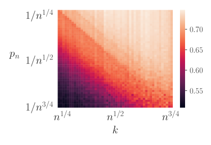
Figure 1: Heatmap showing the AM risk of the balanced $k$-NN.

5.2 Balanced ERM

Now, keeping in mind the fast convergence rate $1/(np)$ obtained in Corollary 4.5, our goal is to show that such a rate is quite sharp as it can be recovered in practice.

We consider the simple setting of a linear classifier defined as $\hat{\beta}_{u}=\hat{g}$ introduced in Section 4 with logistic loss $\ell_{g}(X,Y)=~{}\log(1-e^{-g(X)Y})$, $g(X)=\beta^{T}X$ and $u=10$. Here the sample size $n$ is ranging over the grid $[100,1e4]$ and rare class probability $p=n^{-a}$ while $a\in\{1/3,1/2,2/3\}$.

Some Monte Carlo simulation are needed to estimate $g^{\star}_{\mathrm{bal}}$. We use an $1e{5}$ simulations according to a well balanced data set ($p=1/2$) so that the error computing $g^{\star}_{\mathrm{bal}}$ is sufficiently small. In addition, we use some more Monte Carlo simulation from a balanced test dataset of size $1e4$, to evaluate without bias the risk function $\mathcal{R}_{\mathrm{bal}}$. Based on this, we can obtain both $\mathcal{R}_{\mathrm{bal}}(g^{\star}_{\mathrm{bal}})$ and $\mathcal{R}_{\mathrm{bal}}(\hat{g})$ so that an excess risk value can be obtained. We perform $n_{simu}=1e4$ experiments and we report the average and the upper $0.10$ and $0.90$ quantile of the absolute error obtained over the $n_{simu}$ experiments.

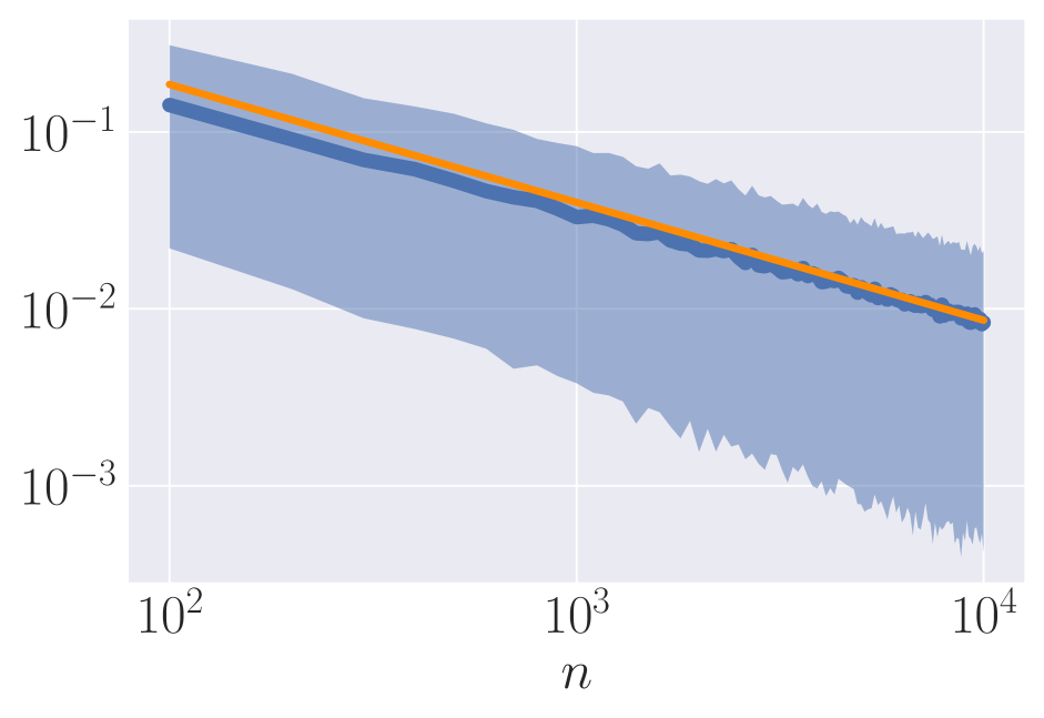
(a) $p_{n}=1/n^{1/3}.$

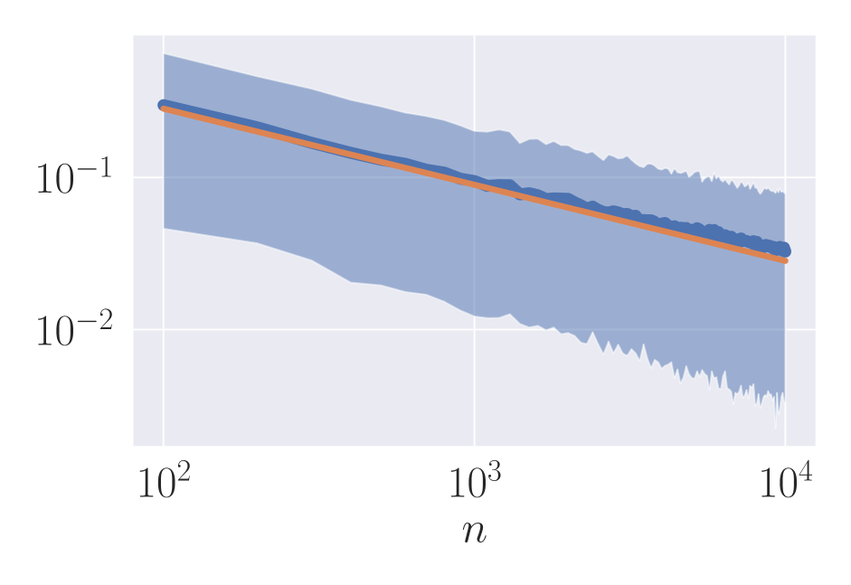
(b) $p_{n}=1/n^{1/2}.$

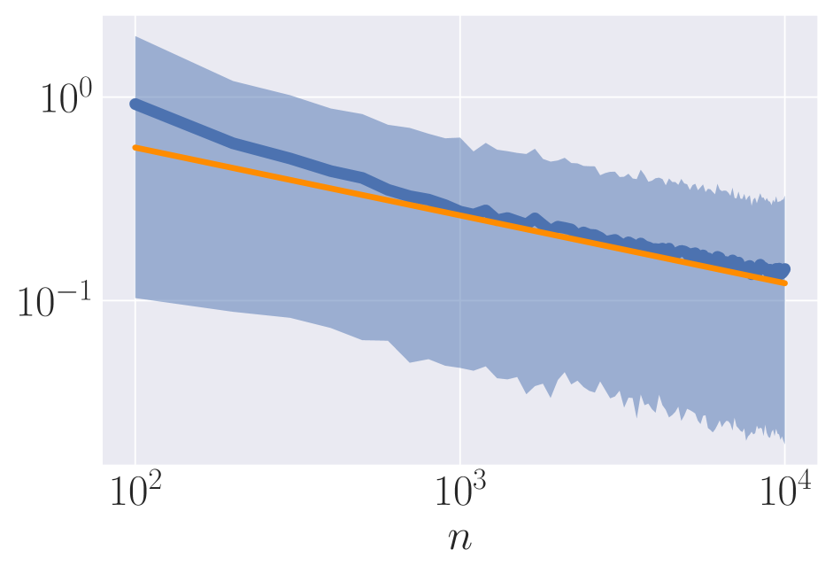
(c) $p_{n}=1/n^{2/3}.$

Figure 2: Excess risk (blue) of logistic regression for different sample size $n$ and the curve $1/np$ (orange). The blue area corresponds to the $0.9$-confidence interval.

.

Figure 2 displays the excess risk as a function of the sample size $n$ in a logarithmic scale, for $a\in\left\{1/3,1/2,2/3\right\}$. Other figures exploring other values of $a$ are reported in the supplementary material. We notice that the excess risk vanishes in the same way as the function $n\mapsto 1/np$ confirming the accuracy of the upper bound from Corollary 4.5.

6 Conclusion

In this paper, we have derived upper bounds for the balanced risk in highly imbalanced classification scenarios. Notably, our bounds remain consistent even under severe class imbalance ($p\to 0$), setting our work apart from existing studies in imbalanced classification (Menon et al.,, 2013; Koyejo et al.,, 2014; Xu et al.,, 2020). Furthermore, it is worth to highlight that this is the first study to achieve fast rates in imbalanced classification, marking a significant advancement in the field.

Our findings corroborate that both risk-balancing approaches and cost-sensitive learning are consistent across nearly all imbalanced classification scenarios. This aligns with experimental works previously documented in the literature (Elkan, 2001b, ; Wang et al.,, 2016; Khan et al.,, 2018; Wang et al.,, 2019; Pathak et al.,, 2022). We also

Furthermore, the methodologies and proof techniques presented in this paper are adaptable to other imbalanced classification metrics beyond balanced classification. Potential extensions include demonstrating consistency for metrics such as the $F_{1}$ measure, recall, and their respective variants.

Appendix A Appendix

A.1 Auxiliary results

The following standard Chernoff inequality is stated and proven in Hagerup and Rüb, (1990).

Theorem A.1.

Let $(Z_{i})_{i\geq 1}$ be a sequence of i.i.d. random variables valued in $\{0,1\}$. Set $\mu=nP(Z_{1})$ and $S=\sum_{i=1}^{n}Z_{i}$. For any $\delta\in(0,1)$ and all $n\geq 1$, we have with probability $1-\delta$:

$$S\geq\left(1-\sqrt{\frac{2\log(1/\delta)}{\mu}}\right)\mu.$$

In addition, for any $\delta\in(0,1)$ and $n\geq 1$, we have with probability $1-\delta$:

$$S\leq\left(1+\sqrt{\frac{3\log(1/\delta)}{\mu}}\right)\mu.$$

The following is taken from Plassier et al., (2023) (see also Giné and Guillou, (2001) for similar uniform bound).

Theorem A.2.

Let $(Z,Z_{1},\ldots,Z_{n})$ be an independent and identically distributed ollection of random variables in $(S,\mathcal{S})$. Let $\mathcal{G}$ be a VC class of functions with parameters $v\geq 1$, $A\geq 1$ and uniform envelope $U\geq\sup_{g\in\mathcal{G},\,x\in S}|g(x)|$. Let $\sigma$ be such that $\sigma^{2}\geq\sup_{g\in\mathcal{G}}var(g(Z))$ and $\sigma\leq 2U$. For any $n\geq 1$ and $\delta\in(0,1)$, it holds, with probability $1-\delta$,

$$\sup_{g\in\mathcal{G}}\left|\sum_{i=1}^{n}\{g(Z_{i})-\mathbb{E}[g(Z)]\}\right|\\ \leq K^{\prime}\left(\sigma\sqrt{vn\log\left(K^{\prime}\theta/\delta\right)}+Uv\log\left(K^{\prime}\theta/\delta\right)\right),$$ (2)

with $\theta=AU/\sigma$ and $K^{\prime}>0$ a universal constant.

Lemma A.3.

Suppose that $\mathcal{F}$ is of VC-type with envelop $U$ and parameter $(v,A)$, then

1. $\{fI_{C}\,:\,f\in\mathcal{F}\}$ is of VC-type with envelop $U$ and parameter $(v,A)$.

2. $\{f-P_{C}(f)\,:\,f\in\mathcal{F}\}$ is of VC-type with envelop $2U$ and parameter $(2v,A)$.

Proof.

Let $Q$ be a probability measure on $(S,\mathcal{S})$. Let $(f_{k})_{k=1,\ldots,K}$ be the center of an $\epsilon U$-covering of $(\mathcal{F},Q)$. The first result follows from the fact that $\|f1_{C}-f_{k}1_{C}\|_{L_{2}(Q)}\leq\|f-f_{k}\|_{L_{2}(Q)}$. Now let $(\tilde{f}_{k})_{k=1,\ldots,K}$ be the center of an $\epsilon U$-covering of $(\mathcal{F},P_{C})$. Consider the covering induces by the centers $(f_{k}-P_{C}(\tilde{f}_{j}))_{1\leq k,j\leq K}$ made of $K^{2}$ elements. Suppose that $f\in\mathcal{F}$. Then there is $k$ and $j$ such that

$$\|(f-P_{C}(f))-(f_{k}-P_{C}(\tilde{f}_{j})\|_{L_{2}(Q)} \leq\|f-f_{k}\|_{L_{2}(Q)}+P_{C}(f-\tilde{f}_{j})$$

$$\leq\|f-f_{k}\|_{L_{2}(Q)}+\|f-\tilde{f}_{j}\|_{L_{2}(P)}$$

$$\leq 2U\epsilon.$$

Hence we have found a $2U\epsilon$-covering of size $K^{2}$ which by assumption is smaller than $(A/\epsilon)^{2v}$. This implies the second statement of the lemma.

∎

The next lemma generalizes Theorem 17.1 from Biau and Devroye, (2015) to the balanced type classifiers.

Lemma A.4.

For any classifier $g$ that writes $g(x)=\operatorname{sign}(\nu(x)-1)$, $x\in\mathcal{X}$, we have

$$\mathcal{R}_{bal}^{*}(g)-\mathcal{R}_{bal}^{*}(g^{*}_{bal})=\mathbb{E}\left[\mathds{1}_{g(X)\neq g^{*}(X)}\frac{\lvert\eta(X)-p\rvert}{p(1-p)}\right],$$

where $g^{*}_{bal}$ is the balanced Bayes classifier (introduced in Section 2). Furthermore, whenever $p\leq 1/2$,

$$\mathcal{R}_{bal}^{*}(g)-\mathcal{R}_{bal}^{*}(g^{*}_{bal})\leq 2\mathbb{E}\left[\left|\nu(X)-\nu^{*}(X)\right|\right]$$

where $\nu^{*}(x)={\eta(x)}/{p}$.

Proof.

The balanced risk writes as

$$\mathcal{R}_{bal}^{*}(g) =P_{+}\left(\nu(X)<1\right)+P_{-}\left(\nu(X)\geq 1\right)$$

$$=\mathbb{E}\left[\frac{\mathbb{I}_{(\nu(X)<1)}\mathbb{I}_{Y=1}}{p}+\frac{\mathbb{I}_{(\nu(X)\geq 1)}\mathbb{I}_{Y=-1}}{1-p}\right].$$

In addition, using a conditioning argument yields,

$$\mathcal{R}_{bal}^{*}(g)=\mathbb{E}\left[\frac{\mathbb{I}_{(\nu(X)<1)}\eta(X)}{p}+\frac{\mathbb{I}_{(\nu(X)\geq 1)}(1-\eta(X))}{1-p}\right].$$

Similarly we have

$$\mathcal{R}_{bal}^{*}(g^{*})=\mathbb{E}\left[\frac{\mathbb{I}_{(\nu^{*}(X)<1)}\eta(X)}{p}+\frac{\mathds{1}_{(\nu^{*}(X)\geq 1)}(1-\eta(X))}{1-p}\right].$$

It follows that

$$\mathcal{R}_{bal}^{*}(g)-\mathcal{R}_{bal}^{*}(g^{*}) =\mathbb{E}\left[\mathbb{I}_{\operatorname{sign}(\nu^{*}(X)-1)\neq\operatorname{sign}(\nu(X)-1)}\frac{\lvert\eta(X)-p\rvert}{p(1-p)}\right]$$

$$=\mathbb{E}\left[\mathbb{I}_{g^{*}(X)\neq g(X)}\frac{\lvert\eta(X)-p\rvert}{p(1-p)}\right],$$

This concludes the first part. For the second part, it remains to note that for any real numbers $(x,y)$

$$\operatorname{sign}(x-1)\neq\operatorname{sign}(y-1)\implies\lvert y-1\rvert\leq\lvert x-y\rvert,$$

so that, using that $\nu^{*}=\eta^{*}/p$, we obtain

$$\mathcal{R}_{bal}^{*}(g)-\mathcal{R}_{bal}^{*}(g^{*}) =\mathbb{E}\left[\mathbb{I}_{\operatorname{sign}(\nu^{*}(X)-1)\neq\operatorname{sign}(\nu(X)-1)}\frac{\lvert\eta(X)-p\rvert}{p(1-p)}\right]$$

$$=\mathbb{E}\left[\mathbb{I}_{\operatorname{sign}(\nu^{*}(X)-1)\neq\operatorname{sign}(\nu(X)-1)}\frac{\lvert\nu^{*}(X)-1\rvert}{(1-p)}\right]$$

$$\leq\frac{\mathbb{E}\left[\lvert\nu^{*}(X)-\nu(X)\rvert\right]}{1-p},$$

but since $p\leq 1/2$ we obtain the desired result.

∎

A.2 Standard rates proof

A.2.1 Proof of Theorem 3.2

Starting with

$$P_{n,+}\left(f\right)-P_{+}\left(f\right)=\frac{P_{n}\left(\left(f-P_{+}\left(f\right)\right)\mathds{1}_{\left\{Y=1\right\}}\right)}{p_{n}}$$ (3)

we focus on each term, denominator and numerator, separately. For the numerator, the term $\left(f-P_{+}(f)\right)\mathds{1}_{\left\{Y=1\right\}}$ has mean $0$. In virtue of Lemma A.3, the class $(f-P_{+}(f))\mathds{1}_{\left\{Y=1\right\}}$ is still bounded by $2U$ and is still VC with VC parameter $(2v,A)$. As a consequence, we can use Proposition 2 in Plassier et al., (2023), stated as Theorem A.2 in the present supplementary file. The variance is bounded as follows

$$\mathrm{Var}\left(\left(f-P_{+}(f)\right)\mathds{1}_{\left\{Y=1\right\}}\right)\leq P\left((f-P_{+}(f))^{2}\mathds{1}_{\left\{Y=1\right\}}\right)=\mathrm{Var}_{+}(f)p=\sigma_{+}^{2}p,$$

by definition of $\sigma_{+}^{2}$. As a consequence, Theorem A.2 gives that

$$P_{n}\left(\left(f-P_{+}(f)\right)\mathds{1}_{\left\{Y=1\right\}}\right)$$

$$\leq K^{\prime}\left(\sqrt{\frac{v\sigma_{+}^{2}p}{n}\log\left(K^{\prime}A/\left(2\delta\sqrt{p}\right)\right)}+\frac{Uv}{n}\log\left(K^{\prime}A/\left(2\delta\sqrt{p}\right)\right)\right)$$

$$\leq 2K^{\prime}\sqrt{\frac{v\sigma_{+}^{2}p}{n}\log\left(K^{\prime}A/\left(2\delta\sqrt{p}\right)\right)},$$

where the last inequality has been obtained using the stated condition on $n$ and $\delta$. For the denominator, using Theorem A.1 we have that, with probability $1-\delta$,

$$\frac{p_{n}}{p}\geq\left(1-\sqrt{\frac{2\log(1/\delta)}{np}}\right)\geq 1/2$$

where the last inequality has been obtained using the condition on $n$ and $\delta$. Using the union bound, we get, with probability $1-2\delta$,

$$\frac{P_{n}\left(\left(f-P_{+}(f)\right)\mathds{1}_{\left\{Y=1\right\}}\right)}{p_{n}}\leq 4K^{\prime}\sqrt{\frac{v\sigma_{\mathcal{F},C}^{2}}{np}\log\left(K^{\prime}A/\left(2\delta\sqrt{p}\right)\right)}$$

and the proof is complete.

A.2.2 Proof of Corollary 3.3

First, using the definition of $\hat{g}_{\mathrm{bal}}$ yields

$$\mathcal{R}_{n,\mathrm{bal}}\left(\hat{g}_{\mathrm{bal}}\right)-\mathcal{R}_{n,bal}\left(g^{*}_{\mathrm{bal}}\right)\leq 0,$$

So that,

$$\mathcal{R}_{\mathrm{bal}}(\hat{g}_{\mathrm{bal}})-\mathcal{R}(g^{*}_{\mathrm{bal}}) \leq\mathcal{R}_{\mathrm{bal}}(\hat{g}_{\mathrm{bal}})-\mathcal{R}_{n,bal}(\hat{g}_{\mathrm{bal}})-\left(\mathcal{R}_{\mathrm{bal}}(g^{*}_{\mathrm{bal}})-\mathcal{R}_{n,\mathrm{bal}}(g^{*}_{\mathrm{bal}})\right)$$

$$\leq\sup_{g\in\mathcal{G}}\left\lvert\mathcal{R}_{\mathrm{bal}}(g)-\mathcal{R}_{n,\mathrm{bal}}(g)\right\rvert$$

$$\leq\sup_{g\in\mathcal{G}}\left|P_{n,-}(g)-P_{-}(g)\right|+\sup_{g\in\mathcal{G}}\left|P_{n,+}(g)-P_{+}(g)\right|.$$

It remains to use Theorem 3.2 and the proof is complete.

A.2.3 Proof of Theorem 3.4

First we recall three results that will be useful in the proof. The following Lemma (Portier,, 2021, Lemma 4) controls the size of the $k$-NN balls uniformly over all $x\in S_{X}$.

Lemma A.5 (Portier, (2021, Lemma 4)).

Suppose that (X1) (X2) and (X3) hold true. Then for all $n\geq 1$, $\delta\in(0,1)$ and $1\leq k\leq n$ such that $24d\log(12n/\delta)\leq k\leq T^{d}nb_{X}cV_{d}/2$ , it holds, with probability at least $1-\delta$:

$$\sup_{x\in S_{X}}\hat{\tau}_{n,k,x}\leq\overline{\tau}_{n,k}:=\left(\frac{2k}{nb_{X}cV_{d}}\right)^{1/d},$$ (4)

where $V_{d}=\lambda(B(0,1))$.

The following lemma is a simple consequence of Theorem A.1.

Lemma A.6.

Let $z_{n}=\sqrt{2\log(1/\delta)/(np)}$. We have with probability at least $1-\delta$,

$$\frac{p}{p_{n}}-1\leq\frac{z_{n}}{1-z_{n}}.$$ (5)

The next lemma is a consequence of Theorem A.2. Let

$$\mathcal{G}=\{g(Y,X)=(\mathds{1}_{Y=1}-\eta(X))\mathbb{I}_{\|X-x\|\leq\tau}:\tau\leq\overline{\tau}_{n,k},\,x\in\mathbb{R}^{d}\}$$

which is of VC type as shown in Lemma 9 in Portier, (2021) (see also Wenocur and Dudley, (1981)). Because $S_{X}$ is compact and $\eta/p$ continuous, there exists $C$ such that $\eta(x)\leq pC$ for all $x\in S_{X}$. The variance of each element in the class is bounded as

$$\mathrm{Var}(g(Y,X))\leq E(\mathds{1}_{Y=1}\mathbb{I}_{\|X-x\|\leq\tau})\leq\int\eta(z)\mathbb{I}_{\|z-x\|\leq\tau}f_{X}(z)dz\leq CpU_{X}\overline{\tau}_{n,k}^{d}V_{d}.$$

Injecting the previous variance bound (which is scales as $pk/n$) in the upper-bound given in Theorem A.2 we obtain the following statement.

Lemma A.7.

We have with probability at least $1-\delta$,

$$\sup_{g\in\mathcal{G}}\left|\sum_{i=1}^{n}g(Y_{i},X_{i})\right|\leq C_{1}(\sqrt{kp\log(C_{2}/\delta)}+\log(C_{2}/\delta))$$ (6)

where $C_{1}$ and $C_{2}$ are constants that does not depend on $n$, $k$ and $p$ (but on the dimension $d$, the VC parameter of $\mathcal{G}$, and the probability measure $P_{X}$).

Define the event $E_{n}$ as the union of (4), (5) and (6). By the previous three lemmas and the union bound $P(E_{n})\geq 1-3\delta$. In light of Borel-Cantelli Lemma we choose $\delta=1/n^{2}$ so that $\sum_{n}(1-P(E_{n}))$ is finite and the event $\liminf_{n}E_{n}$ has probability $1$. It then suffices to show that $E_{n}$ implies that ${\hat{\eta}_{n}(x)}/{p_{n}}-\nu^{*}(x)=O(\sqrt{\log(n)/kp}+(k/n)^{1/d})$. Note that under $E_{n}$, when $n$ is large enough, by (5), $p/p_{n}\leq 2$. Let $M_{i}=\mathds{1}_{Y_{i}=1}-\eta(X_{i})$ and $B_{i}(x)=\eta(X_{i})-\eta(x)$. We have

$$\frac{\hat{\eta}_{n}(x)}{p_{n}}-\nu^{*}(x)= \frac{\sum_{i\in I_{n}(x)}M_{i}}{kp_{n}}+\frac{\sum_{i\in I_{n}(x)}B_{i}(x)}{kp_{n}}+\eta(x)\left(\frac{1}{p_{n}}-\frac{1}{p}\right).$$ (7)

On the event $E_{n}$, the function $(Y,X)\mapsto(\mathds{1}_{Y=1}-\eta(X))\mathds{1}_{\|X-x\|\leq\hat{\tau}_{n,k,x}}$ belongs to the space $\mathcal{G}$. Consequently, the first term in (7) is smaller than

$$(kp_{n})^{-1}\sup_{g\in\mathcal{G}}\left|\sum_{i=1}^{n}g(Y_{i},X_{i})\right|$$

which by (5) and (6) is $O(\sqrt{\log(n)/kp})$. Using the assumption that $x\mapsto\eta(x)/p$ is $L$-Lipschitz we get that, on $E_{n}$, the second term in (7) is such that

$$\frac{\sum_{i\in I_{n}(x)}B_{i}(x)}{kp_{n}}\leq\frac{p}{p_{n}}L\overline{\tau}_{n,k},$$

which, using (5), is $O((k/n)^{1/d})$. The third term in (7) is smaller than $\left(\eta(x)/p\right)\left(p/p_{n}-1\right)$ which is, using again the Lipschitz assumption and (5), $O(\sqrt{\log(n)/(np)}$. The latter bound is smaller than $\sqrt{\log(n)/(kp)}$ so it does not appear in the stated bound.

A.3 Fast rates proofs

Before moving to the main proof we remind some necessary notions. First, let’s recall the definitions of sub-root functions:

Definition A.8.

A function $\psi:[0,\infty)\rightarrow[0,\infty)$ is sub-root if it is nonnegative, nondecreasing and if $r\mapsto\psi(r)/\sqrt{r}$ is nonincreasing for $r>0$.

In the sequel, we will focus on a specific type of functions, given by:

$$\phi_{\mathcal{F}}(r)=P\left(R_{n}\left\{f\in\mathcal{F}\mid P_{n}f^{2}\leq r\right\}\right)$$

where $R_{n}\left(\mathcal{F}\right)=\frac{1}{n}\sup_{f\in\mathcal{F}}\sum_{i=1}^{n}\sigma_{i}f(X_{i})$ denotes the empirical Rademacher complexity for a given realisation of $\sigma_{i}$’s, $X_{i}$’s. The expectation in this formulation is with respect to the budget of samples $(X_{i},Y_{i})_{1\leq i\leq n}$ and the Rademacher chaos variables $\sigma_{i}$’s. Remember that $\sigma_{i}\in\left\{-1,1\right\}$ and $P(\sigma_{i}=\pm 1)=\frac{1}{2}$.
At this point, it is important to mention that if we define $\mathcal{G}=star(\mathcal{F},0)$ as the star-hull of $\mathcal{F}$ centered around $0$, that is,

$$\mathcal{G}=star(\mathcal{F},0)=\left\{\alpha f\mid\alpha\in[0,1],f\in\mathcal{F}\right\},$$

then the function $\phi_{\mathcal{G}}$ is sub-root (see e.g. Lemma 3.4 in Bartlett et al., (2005)). In the next lemma we derive an upper bound for $\phi_{\mathcal{G}}(2r)$, which is a crucial quantity in the proof of Theorem 4.1.

Lemma A.9.

Let $\mathcal{F}$ be a class of functions that is VC-type with envelop $U\geq 1$ and parameter $v,A\geq 1$. Set $\mathcal{G}$ to be the star-hull of $\mathcal{F}$ around $0$. Then, the Rademacher complexity $\phi_{\mathcal{G}}(2r)$ verifies

$$\phi_{\mathcal{G}}(2r)=P\left(R_{n}\left\{g\in\mathcal{G}\mid P_{n}g^{2}\leq 2r\right\}\right)\leq CD\log\left(\frac{8AU}{r}\right)\sqrt{\frac{v+1}{n}}\sqrt{r}.$$

Where $D_{1}=8^{1/v}CAUC_{1}C_{2}$, $C>0$ is a universal constant, $C_{1}=\frac{1}{\sqrt{\log(8A)}}$ and $C_{2}=\sqrt{2}\left(\max\left(\frac{\log\left(4AU\right)}{\log\left(8A\right)},1\right)+\sqrt{2}\right)$ .

Proof.

By definition of $\mathcal{G}$, any element $g\in\mathcal{G}$ verifies $P_{n}g^{2}\leq U^{2}$, thus for $r\geq\frac{U^{2}}{2}$ the function $\phi_{\mathcal{G}}(r)$ is constant. Therefore if the latter inequality holds for $r\leq\frac{U^{2}}{2}$ it automatically extends to the case $r\geq\frac{U^{2}}{2}$. Thus, in the sequel we assume that $r\leq\frac{U^{2}}{2}$.

Using classical results (see e.g. the discussion following Lemma 7.3 in Van Handel, (2014) ) one has, for some universal constant $C>0$,

$$P_{\sigma}\left[R_{n}(\mathcal{G}_{2r})\right]\leq\frac{C}{\sqrt{n}}\int_{0}^{\infty}\sqrt{\log\mathcal{N}\left(\mathcal{G}_{2r},L_{2}(P_{n}),\epsilon\right)}d\epsilon,$$

which yields,

$$P\left(R_{n}(\mathcal{G}_{2r})\right)\leq P\left(\frac{C}{\sqrt{n}}\int_{0}^{\infty}\sqrt{\log\mathcal{N}\left(\mathcal{G}_{2r},L_{2}(P_{n}),\epsilon\right)}d\epsilon\right),$$

where $\mathcal{G}_{r}=\left\{g\in\mathcal{G}\mid P_{n}g^{2}\leq r\right\}$ and $C>0$ is a universal constant. By definition of $\mathcal{G}_{r}$, the covering number of the latter class verifies $\mathcal{N}\left(\mathcal{G}_{r},L_{2}(P_{n}),\epsilon\right)=1$ as soon as $\epsilon\geq\sqrt{r}$. Therefore,

$$P\left(R_{n}(\mathcal{G}_{2r})\right) \leq\frac{C}{\sqrt{n}}P\left(\int_{0}^{\sqrt{2r}}\sqrt{\log\mathcal{N}\left(\mathcal{G}_{2r},L_{2}(P_{n}),\epsilon\right)}d\epsilon\right)$$

$$(\mathcal{G}_{2r}\subset\mathcal{G}) \leq\frac{C}{\sqrt{n}}P\left(\int_{0}^{\sqrt{2r}}\sqrt{\log\mathcal{N}\left(\mathcal{G},L_{2}(P_{n}),\epsilon\right)}d\epsilon\right)$$

$$\leq\frac{C}{\sqrt{n}}P\left(\int_{0}^{\sqrt{2r}}\sqrt{\log\left(\mathcal{N}\left(\mathcal{F},L_{2}(P_{n}),\frac{\epsilon}{2}\right)\left(\frac{4}{\epsilon}\right)\right)}d\epsilon\right).$$ (8)

Where the last line follows from Lemma 4.5 in Mendelson, (2002). On the other hand, using the VC assumption we obtain

$$\forall\epsilon\leq\sqrt{2r}\,,\,\mathcal{N}\left(\mathcal{F},L_{2}(P_{n}),\epsilon\right)\leq 2\left(\frac{AU}{\epsilon}\right)^{v}.$$

So that

$$\log\left(\mathcal{N}\left(\mathcal{F},L_{2}(P_{n}),\epsilon/2\right)\left(\frac{4}{\epsilon}\right)\right) \leq(v+1)\log\left(\frac{(AU)^{\frac{v}{v+1}}8^{1/v}}{\epsilon}\right)$$

$$\left(A\geq 1\,,\,U\geq 1\right) \leq(v+1)\log\left(\frac{8AU}{\epsilon}\right).$$

Therefore, Inequality (A.3) becomes

$$P\left(R_{n}(\mathcal{G}_{2r})\right) \leq C\sqrt{\frac{v+1}{n}}\int_{0}^{\sqrt{2r}}\sqrt{\log\left(\frac{8AU}{\epsilon}\right)}d\epsilon$$

$$\leq CC_{1}\sqrt{\frac{v+1}{n}}\int_{0}^{\sqrt{2r}}\log\left(\frac{8AU}{\epsilon}\right)d\epsilon$$

$$\leq 8^{1/v}AUCC_{1}\sqrt{\frac{v+1}{n}}\int_{0}^{\sqrt{2r/(8^{1/v}AU)^{2}}}\log\left(\frac{1}{\epsilon}\right)d\epsilon.$$

$$\left(8^{1/v}\leq 8\right) \leq 8^{1/v}AUCC_{1}\sqrt{\frac{v+1}{n}}\int_{0}^{\sqrt{2r/(8AU)^{2}}}\log\left(\frac{1}{\epsilon}\right)d\epsilon.$$

Where $C_{1}=\frac{1}{\sqrt{\log(8A)}}>0$. Indeed, the second inequality follows since

$$\forall r\leq\frac{U^{2}}{2}\,,\,\forall\epsilon\leq\sqrt{2r}\,,\,\sqrt{\log\left(\frac{8AU}{\sqrt{\epsilon}}\right)}\leq C_{1}\log\left(\frac{\displaystyle 8AU}{\displaystyle\sqrt{\epsilon}}\right).$$

Besides, $\int\log\left(\frac{1}{x}\right)=-\int\log(x)=x\log\left(\frac{1}{x}\right)+x$ which yields,

$$P\left(R_{n}(\mathcal{G}_{2r})\right)\leq 8^{1/v}AUCC_{1}C_{2}\log\left(\frac{8AU}{r}\right)\sqrt{\frac{v+1}{n}}\sqrt{r}.$$ (9)

For some constant $C_{2}=\sqrt{2}\left(\max\left(\frac{\log\left(4AU\right)}{\log\left(8A\right)},1\right)+\sqrt{2}\right)>0$. Indeed, by considering the cases $r\geq\sqrt{2r}$, $r\leq\sqrt{2r}$ and by simple algebra one has

$$\forall r\leq\frac{U^{2}}{2}\,,\,\sqrt{2r}\log\left(\frac{8AU}{\sqrt{2r}}\right)+\sqrt{2r}\leq C_{2}\sqrt{r}\log\left(\frac{\displaystyle 8AU}{\displaystyle r}\right).$$

In fact, $r\leq\sqrt{2r}$ implies$\frac{1}{\sqrt{2r}}\leq\frac{1}{r}$ and $r\leq 2$, so that

$$\begin{cases}\sqrt{r}\log\left(\frac{8AU}{r}\right)&\geq\sqrt{r}\log\left(\frac{8AU}{\sqrt{2r}}\right)\\ \sqrt{r}\log\left(\frac{8AU}{r}\right)&\geq\sqrt{r}\log\left(4AU\right)\end{cases}.$$

On the other hand, $r\geq\sqrt{2r}$ implies $r\geq 2$. Now, remind that $r\leq\frac{U^{2}}{2}$ and write

$$\begin{cases}\log\left(\frac{8AU}{r}\right)&\geq\log\left(8A\right)\\ \log\left(\frac{8AU}{\sqrt{2r}}\right)&\leq\log\left(4AU\right)\leq\log\left(4AU\right)\log\left(\frac{8AU}{r}\right)/\log\left(8A\right)\end{cases},$$

which yields the desired result. ∎

The proof of Theorem 4.1 relies on applying Theorem 3.3 in Bartlett et al., (2005) recalled for completeness below.

Theorem A.10.

Let $\mathcal{F}$ be a class of functions with ranges in $[a,b]$ and assume that there are some functional $T:\mathcal{F}\rightarrow\mathbb{R}^{+}$and some constant $B$ such that for every $f\in\mathcal{F},\operatorname{Var}[f]\leq T(f)\leq BPf$. Let $\psi$ be a sub-root function and let $r^{\star}$ be the fixed point of $\psi$, i.e. $\psi(r^{\star})=r^{\star}$ . Assume that $\psi$ satisfies, for any $r\geq r^{\star}$,

$$\psi(r)\geq BP\left(R_{n}\{f\in\mathcal{F}:T(f)\leq r\}\right)$$

Then, with $c_{1}=704$ and $c_{2}=26$, for any $K>1$ and every $x>0$, with probability at least $1-e^{-x}$,

$$\forall f\in\mathcal{F}\quad Pf\leq\frac{K}{K-1}P_{n}f+\frac{c_{1}K}{B}r^{\star}+\frac{x\left(11(b-a)+c_{2}BK\right)}{n}.$$

Also, with probability at least $1-e^{-x}$,

$$\forall f\in\mathcal{F}\quad P_{n}f\leq\frac{K+1}{K}Pf+\frac{c_{1}K}{B}r^{\star}+\frac{x\left(11(b-a)+c_{2}BK\right)}{n}.$$

Furthermore if the functional $T$ verifies $T(\alpha f)\leq\alpha^{2}T(f)$ then the same inequalities holds with $c_{2}=6$ and $c_{1}=5$.

Let us now demonstrate a direct corollary of Lemma 7 from Cucker et al., (2002), which will enable us to establish an upper bound for the fixed point $r^{\star}$ featured in the aforementioned expression.

Corollary A.11.

Let $x,s,q,a,b>0$ such as $s\geq q$ and $x^{s}\leq ax^{q}+b.$ Then,

$$x\leq\max\left((2a)^{\frac{1}{s-q}},(2b)^{\frac{1}{s}}\right).$$

Proof.

By Lemma 7 in Cucker et al., (2002) the equation $x^{s}-ax^{q}+b=0$ has a unique solution $x^{\star}$ verifying,

$$x^{\star}\leq\max\left((2a)^{\frac{1}{s-q}},(2b)^{\frac{1}{s}}\right).$$

Furthermore , since $s\geq q$ the function $x\mapsto x^{s}-ax^{q}+b$ is continuous negative at $0$ and positive at $+\infty$. Therefore,

$$x^{s}\leq ax^{q}+b\implies x\leq x^{\star},$$

and the result follows.

∎

To conclude this section, Let’s provide a useful lemma that establishes a connection between the VC dimension of the class $\widetilde{\mathcal{F}}=\left\{\frac{1}{2}fI_{1}+\frac{1}{2}\frac{p}{1-p}fI_{-1}\mid f\in\mathcal{F}\right\}$ and the VC dimension of $\mathcal{F}$.

Lemma A.12.

If a family $\mathcal{F}$ of functions is of VC-type with envelop $U$ and parameter $(v,A)$, then if $p\leq\frac{1}{2}$, the family $\widetilde{\mathcal{F}}=\left\{\frac{1}{2}fI_{1}+\frac{1}{2}\frac{p}{1-p}fI_{-1}\mid f\in\mathcal{F}\right\}$ is also VC-type with envelop $U$ and parameter $(v,A)$.

Proof.

Let $0<\epsilon\leq 1$, $p=P(C)$ and $f_{k},k=1,\ldots,N_{\mathcal{F}}$ be an $\epsilon$ covering of $\mathcal{F}$ for a norm $\left|\right|$. Take an element $g$ of $\widetilde{\mathcal{F}}$ which writes $g=\frac{1}{2}fI_{1}+\frac{1}{2}\frac{p}{1-p}fI_{-1}$ for some $f\in\mathcal{F}$ and notice that there exists some $k$ such as $\left\|f-f_{k}\right\|\leq\epsilon$. Thus, by setting $g_{k}=\frac{1}{2}f_{k}I_{1}+\frac{1}{2}\frac{p}{1-p}f_{k}I_{-1}\in\widetilde{\mathcal{F}}$, one has

$$\left\|g-g_{k}\right\|\leq\frac{1}{2}\left\|f_{k}-f\right\|+\frac{1}{2}\frac{p}{1-p}\left\|(f_{k}-f)\right\|\leq\epsilon\left(\frac{1}{2}+\frac{1}{2}\frac{p}{1-p}\right)\leq\epsilon.$$

Indeed $p\leq\frac{1}{2}$ implies $\frac{p}{1-p}\leq 1$. The latter fact implies that the covering number of $\mathcal{F}$ and $\widetilde{\mathcal{F}}$ is the same and the proof is complete. ∎

A.3.1 Proof of Theorem 4.1

This proof follows a line of reasoning similar to the proofs of Corollary 3.7 in Bartlett et al., (2005) and Theorem 2.12 in Bartlett and Mendelson, (2006) which holds only for the class of binary functions. The proof consists on using Theorem A.10 and upper bounding the term $r^{*}$ appearing in the display of the latter theorem. To do so set

$$\widetilde{\mathcal{F}}=\left\{\frac{1}{2}fI_{1}+\frac{1}{2}\frac{p}{1-p}fI_{-1}\mid f\in\mathcal{F}\right\},$$

and let $\mathcal{G}=star\left(\widetilde{\mathcal{F}},0\right)$. Now, consider the following sub-root function

$$\psi_{\mathcal{G}}(r)=10B_{U}P\left(R_{n}\left\{g\in\mathcal{G}\mid P_{n}g^{2}\leq 2r\right\}\right)+\frac{11B_{U}^{2}\log(n)+B_{U}^{2}}{n},$$ (10)

with $B_{U}=\max(B,U)$. Since $\mathcal{F}$ is VC, Lemma A.12 allows to use Lemma A.11 on $\mathcal{G}$ to obtain

$$\psi_{\mathcal{G}}(r)\leq 10B_{U}D_{1}\sqrt{\frac{v+1}{n}}\sqrt{r}\log\left(\frac{8AU}{r}\right)+\frac{11B_{U}^{2}\log(n)+B_{U}^{2}}{n}.$$

Now, remind that by definition $\psi_{\mathcal{G}}(r)\geq\frac{\displaystyle B_{U}^{2}}{\displaystyle n}$ thus $r^{\star}=\psi_{\mathcal{G}}(r^{\star})\geq\frac{\displaystyle B_{U}^{2}}{\displaystyle n}\geq\frac{\displaystyle U^{2}}{\displaystyle n}$ and the latter inequality becomes,

$$r^{\star}=\psi_{\mathcal{G}}(r^{\star})\leq 10B_{U}D_{1}\sqrt{\frac{v+1}{n}}\sqrt{r^{\star}}\log\left(\frac{8An}{U}\right)+\frac{11U^{2}\log(n)+U^{2}}{n}.$$

So that by Corollary A.11

$$r^{\star}\leq 20B_{U}D_{1}\frac{\displaystyle v+1}{\displaystyle n}\log\left(\frac{8An}{U}\right)^{2}.$$ (11)

But, Corollary 2.2 in Bartlett et al., (2005) states that, for any $r$ such as

$$r\geq u_{n}:=10UP\left(R_{n}\left\{g\in\mathcal{G}\mid P_{n}g^{2}\leq 2r\right\}\right)+\frac{11U^{2}\log(n)}{n},$$

one has with probability $1-\frac{\displaystyle 1}{\displaystyle n}$,

$$\left\{g\in\mathcal{G}\mid Pg^{2}\leq r\right\}\subset\left\{g\in\mathcal{G}\mid P_{n}g^{2}\leq 2r\right\}.$$

On the other hand, by Assumption 4.2 the family $\mathcal{G}$ is $U$ bounded. Therefore, one has $R_{n}\left\{g\in\mathcal{G}\mid Pg^{2}\leq r\right\}\leq U$ and for any $r\geq u_{n}$,

$$P\left(R_{n}\left\{g\in\mathcal{G}\mid Pg^{2}\leq r\right\}\right)\leq\left(1-\frac{1}{n}\right)P\left(R_{n}\left\{g\in\mathcal{G}\mid P_{n}g^{2}\leq 2r\right\}\right)+\frac{U}{n}.$$

Remind that, by definition of $\psi_{\mathcal{G}}$ (cf. Equation (10)) one has $\psi_{\mathcal{G}}(r)\geq u_{n}$, so that for any $r\geq\psi_{\mathcal{G}}(r)\geq u_{n}$ it holds

$$BP\left(R_{n}\left\{g\in\mathcal{G}\mid Pg^{2}r\right\}\right) \leq BP\left(R_{n}\left\{g\in\mathcal{G}\mid P_{n}g^{2}\leq 2r\right\}\right)+\frac{BU}{n}$$

$$\left(B=\max(B,U)\right) \leq B_{U}P\left(R_{n}\left\{g\in\mathcal{G}\mid P_{n}g^{2}\leq 2r\right\}\right)+\frac{B_{U}^{2}}{n}$$

$$\leq\psi_{\mathcal{G}}(r).$$

Since $\psi_{\mathcal{G}}$ is subroot (as discussed in the introduction of the present section) Lemma 3.2 in the latter reference implies that :

$$r\geq r^{\star}\iff r\geq\psi_{\mathcal{G}}(r).$$

Thus one has,

$$\forall r\geq r^{\star}\,,\,\psi_{\mathcal{G}}(r) \geq BP\left(R_{n}\left\{g\in\mathcal{G}\mid Pg^{2}\leq r\right\}\right)$$ (12)

$$\left(\widetilde{\mathcal{F}}\subset\mathcal{G}\right) \geq BP\left(R_{n}\left\{f\in\widetilde{\mathcal{F}}\mid Pg^{2}\leq r\right\}\right).$$ (13)

In addition, it holds that,

$$\forall\tilde{f}\in\widetilde{\mathcal{F}}\,,\,var\left[\tilde{f}\right]\leq P\left(\tilde{f}^{2}\right)\leq BP\left(\tilde{f}\right).$$

It remains to use Theorem A.10 combined with Inequality (11) to obtain, with $c_{1}=6$, $c_{2}=5$, with probability $1-\delta$

$$\forall f\in\mathcal{F}\quad P\left(\frac{1}{2}fI_{1}+\frac{1}{2}\frac{p}{1-p}fI_{-1}\right) \leq\frac{K}{K-1}P_{n}\left(\frac{1}{2}fI_{1}+\frac{1}{2}\frac{p}{1-p}fI_{-1}\right)$$

$$+\frac{c_{1}K}{B}\frac{D^{\prime}\log(An)^{2}}{n}+\frac{\log(1/\delta)\left(22U+c_{2}BK\right)}{n}.$$

With $D^{\prime}=20B_{U}D_{1}(v+1)$. On the other hand, notice that for any $\tilde{f}=\frac{1}{2}fI_{1}+\frac{1}{2}\frac{p}{1-p}fI_{-1}$ one has $\frac{\displaystyle 1}{\displaystyle p}P\left(\tilde{f}\right)=P_{\mathrm{bal}}(f)$ thus dividing by $p$ the latter inequality yields,

$$\forall f\in\mathcal{F}\quad P_{\mathrm{bal}}(f) \leq\frac{K}{K-1}\times\frac{1}{2}\left(\frac{1}{p}P_{n}(fI_{1})+\frac{1}{1-p}P_{n}(fI_{-1})\right)$$

$$\hskip 50.00008pt+\frac{c_{1}K}{B}\frac{D^{\prime}\log(An)^{2}}{np}+\frac{\log(1/\delta)\left(22U+c_{2}BK\right)}{np}.$$

$$=\frac{K}{K-1}\times\frac{1}{2}\left(P_{n}(f\mid Y=1)\frac{p_{n}}{p}+P_{n}(f\mid Y=-1)\frac{1-p_{n}}{1-p}\right)$$

$$\hskip 50.00008pt+\frac{c_{1}K}{B}\frac{D^{\prime}\log(An)^{2}}{np}+\frac{\log(1/\delta)\left(22U+c_{2}BK\right)}{np}.$$ (14)

Now notice that one has by Theorem A.1, with probability $1-2\delta$,

$$\begin{cases}\vspace{1em}\frac{\displaystyle p_{n}}{\displaystyle p}\leq 1+\sqrt{\frac{\displaystyle 3\log(1/\delta)}{\displaystyle np}}\cr\frac{\displaystyle 1-p_{n}}{\displaystyle 1-p}\leq 1+\sqrt{\frac{\displaystyle 3\log(1/\delta)}{\displaystyle n(1-p)}}\leq 1+\sqrt{\frac{\displaystyle 3\log(1\delta)}{\displaystyle np}}\end{cases}.$$

The last inequaliy follow since $p\leq\frac{1}{2}$. Finally, by union bound and Inequality (A.3.1) one has, with probability $1-3\delta$,

$$\forall f\in\mathcal{F}\quad P_{\mathrm{bal}}(f)\leq\frac{K}{K-1} P_{n,\mathrm{bal}}(f)\Bigg{(}1+\sqrt{\frac{3\log(1/\delta)}{np}}\Bigg{)}$$

$$+\frac{DK}{B}\frac{\log(An)^{2}}{n}+\frac{\log(1/\delta)\left(22U+c_{2}BK\right)}{n}.$$

with $D=c_{1}(v+1)D^{\prime}=C^{\prime}8^{\frac{1}{v}}(v+1)AUC_{1}C_{2}$, $C^{\prime}=20c_{1}=120$. To show the second part and to conclude the proof follow the same reasoning as before and use instead the second statement of Theorem A.10.

A.3.2 Proof of Corollary 4.3

The proof follows in a straightforward way from Theorem 4.1. Since Assumption 4.2 holds, we can apply Theorem 4.1 to the class of functions $\mathcal{F}_{1}=\{\ell_{g}-\ell_{g^{\star}_{\mathrm{bal}}}\,:\,g\in\mathcal{G}\}$ and obtain, with probability $1-3\delta$,

$$\forall g\in\mathcal{G}\quad P_{\mathrm{bal}}(\ell_{g}-\ell_{g^{\star}_{\mathrm{bal}}})\leq\frac{K}{K-1}P_{n,\mathrm{bal}}(\ell_{g}-\ell_{g_{\mathrm{bal}}^{\star}}) \Bigg{(}1+\sqrt{\frac{3\log(1/\delta)}{np}}\Bigg{)}$$

$$+\frac{DK}{B}\frac{\log(An)^{2}}{np}+\frac{\log(1/\delta)\left(c_{2}+c_{1}BK\right)}{np}.$$

In particular for $\hat{g}_{\mathrm{bal}}=\operatorname*{arg\,min}_{g\in\mathcal{G}}\mathcal{R}_{n,\mathrm{bal}}(g)=\operatorname*{arg\,min}_{g\in\mathcal{G}}P_{n,\mathrm{bal}}(g)$, we have

$$P_{n,\mathrm{bal}}\left(\hat{g}_{\mathrm{bal}}-g^{\star}_{\mathrm{bal}}\right)=P_{n,\mathrm{bal}}(\hat{g}_{\mathrm{bal}})-P_{n,\mathrm{bal}}(g^{\star}_{\mathrm{bal}})\leq 0$$

and the result follows by reminding that $P_{\mathrm{bal}}(\ell_{\hat{g}_{\mathrm{bal}}}-\ell_{g^{\star}_{\mathrm{bal}}})=\mathcal{R}_{\mathrm{bal}}(\hat{g}_{\mathrm{bal}})-\mathcal{R}_{\mathrm{bal}}(g^{\star}_{\mathrm{bal}})$ and by taking $K=1$.

A.3.3 Proof of Lemma 4.4

By definition one has,

$$\tilde{\ell}_{g}(X,Y)=\ell_{g}(X,Y)I_{A}+\frac{p}{1-p}\ell_{g}(X,Y)I_{B},$$

confirming that, if $g\mapsto\mathbb{E}\left[\ell_{g}(X,Y)\right]$ is $\lambda$-strongly convex then $g\mapsto\mathbb{E}\left[\tilde{\ell}_{g}(X,Y)\right]$ is $p\lambda$-strongly convex.

Note that $g^{\star}_{\mathrm{bal}}$ minimizes $\mathbb{E}\left[\tilde{\ell}_{g}(X,Y)\right]$, which implies:

$$\mathbb{E}\left[\tilde{\ell}_{g}(X,Y)\right]-\mathbb{E}\left[\tilde{\ell}_{g^{\star}_{\mathrm{bal}}}(X,Y)\right]\geq p\lambda\left\|g-g^{\star}_{\mathrm{bal}}\right\|^{2}.$$

Using the Lipschitz assumption, we obtain:

$$\mathbb{E}\left[\left(\tilde{\ell}_{g}(X,Y)-\tilde{\ell}_{g^{\star}_{\mathrm{bal}}}(X,Y)\right)^{2}\right] \leq L^{2}\left(P(I_{A})+\frac{p^{2}}{(1-p)^{2}}P(I_{B})\right)\left\|g-g^{\star}_{\mathrm{bal}}\right\|^{2},$$

$$(p\leq 1/2) \leq 2pL^{2}\left\|g-g^{\star}_{\mathrm{bal}}\right\|^{2}.$$

The proof is concluded by combining the above inequalities.

A.4 Numerical experiments: Real world dataset

Our aim, just as in the main paper, is to illustrate the decision boundary of the $k$-nn classifiers on real-world datasets. To do so, we follow the same procedure as the main paper, but instead of using synthetic data, we employ six real-world datasets (Pima, Breast, Cardio, Sattelite, Annthyroid, Ionosphere) from the ODDS repository. Figures 4 to 8 display the balanced accuracy ($1-\mathcal{R}^{0-1}_{\mathrm{bal}}$) of the balanced $k$-nn as function of $(k,p)$, we make the proportion of positive class $p$ vary by randomly removing positive examples. Similar to the findings on synthetic data, these experiments suggest that a large number of neighbors $k$ should be chosen relative to $p_{n}$ to ensure the consistency of the nearest neighbors method. It’s important to note, however, that the learning boundary appears somewhat more noisy than in the synthetic data case. This is indeed not surprising since the number of examples available is significantly smaller in comparison to the previous simulation.

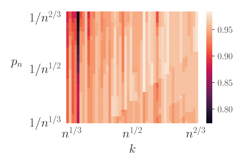
Figure 3: Balanced accuracy heat map for the Breast dataset.

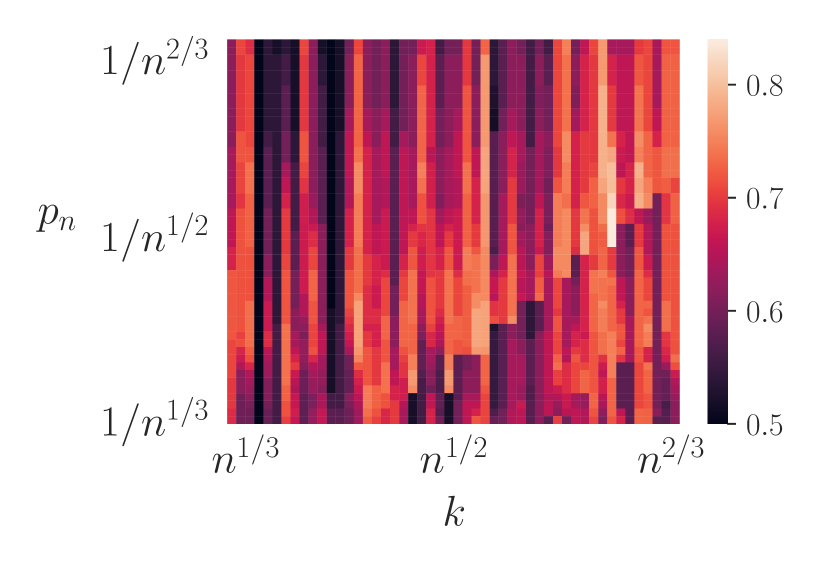
Figure 4: Balanced accuracy heat map for the Ionosphere dataset.

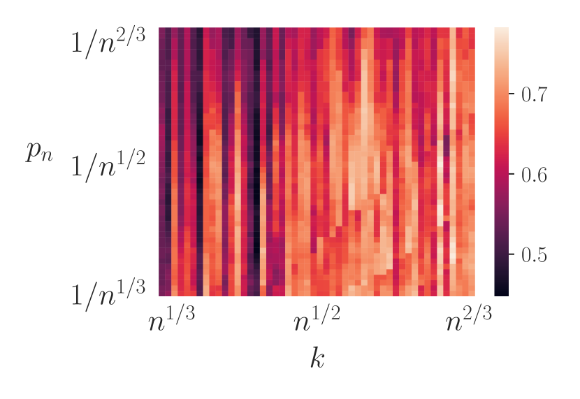
Figure 5: Balanced accuracy heat map for the Pima dataset.

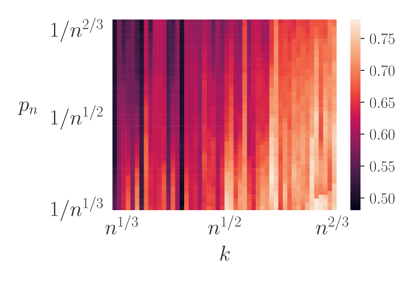
Figure 6: Balanced accuracy heat map for the Annthyroid dataset.

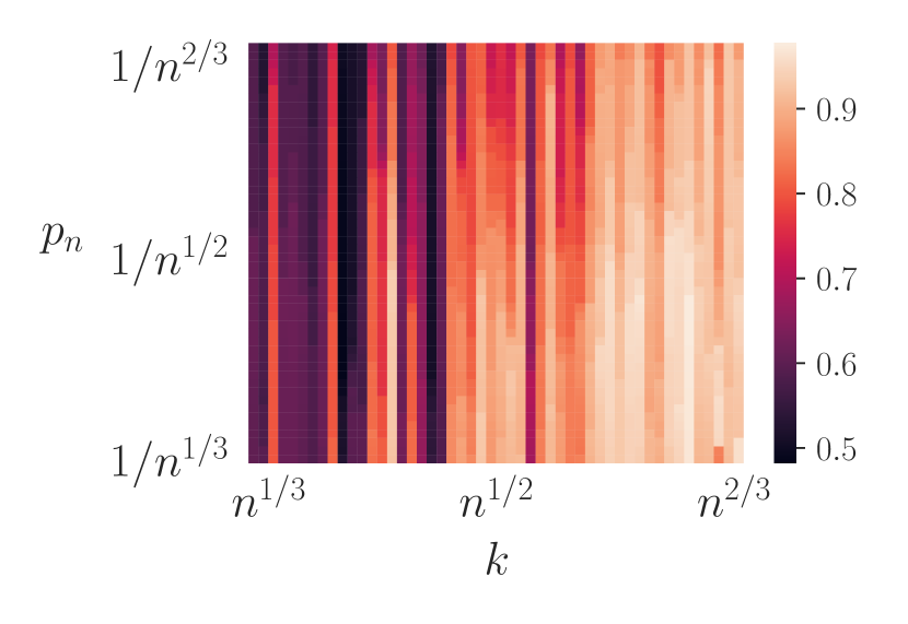
Figure 7: Balanced accuracy heat map for the Cardio dataset.

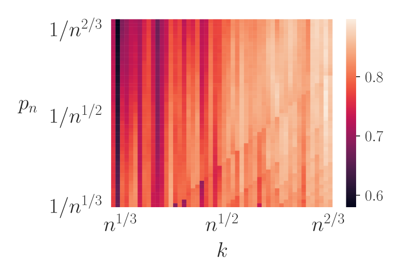
Figure 8: Balanced accuracy heat map for the Satellite dataset.

References

- Agarwal et al., (2018) Agarwal, A., Beygelzimer, A., Dudík, M., Langford, J., and Wallach, H. (2018). A reductions approach to fair classification. In International Conference on Machine Learning, pages 60–69. PMLR.
- Aghbalou et al., (2023) Aghbalou, A., Portier, F., Sabourin, A., and Zhou, C. (2023). Tail inverse regression for dimension reduction with extreme response.
- Bartlett et al., (2005) Bartlett, P. L., Bousquet, O., and Mendelson, S. (2005). Local Rademacher complexities. The Annals of Statistics, 33(4):1497 – 1537.
- Bartlett et al., (2006) Bartlett, P. L., Jordan, M. I., and Mcauliffe, J. D. (2006). Convexity, classification, and risk bounds. Journal of the American Statistical Association, 101(473):138–156.
- Bartlett and Mendelson, (2006) Bartlett, P. L. and Mendelson, S. (2006). Empirical minimization. Probability theory and related fields, 135(3):311–334.
- Bertail et al., (2021) Bertail, P., Clémençon, S., Guyonvarch, Y., and Noiry, N. (2021). Learning from biased data: A semi-parametric approach. In Meila, M. and Zhang, T., editors, Proceedings of the 38th International Conference on Machine Learning, volume 139 of Proceedings of Machine Learning Research, pages 803–812. PMLR.
- Biau and Devroye, (2015) Biau, G. and Devroye, L. (2015). Lectures on the nearest neighbor method, volume 246. Springer.
- Boucheron et al., (2005) Boucheron, S., Bousquet, O., and Lugosi, G. (2005). Theory of classification: A survey of some recent advances. ESAIM: probability and statistics, 9:323–375.
- Chawla et al., (2002) Chawla, N. V., Bowyer, K. W., Hall, L. O., and Kegelmeyer, W. P. (2002). Smote: synthetic minority over-sampling technique. Journal of artificial intelligence research, 16:321–357.
- Cucker et al., (2002) Cucker, F., Smale, S., et al. (2002). Best choices for regularization parameters in learning theory: on the bias-variance problem. Foundations of computational Mathematics, 2(4):413–428.
- (11) Elkan, C. (2001a). The foundations of cost-sensitive learning. Proceedings of the Seventeenth International Conference on Artificial Intelligence: 4-10 August 2001; Seattle, 1.
- (12) Elkan, C. (2001b). The foundations of cost-sensitive learning. In International joint conference on artificial intelligence, volume 17-1, pages 973–978. Lawrence Erlbaum Associates Ltd.
- Fu et al., (2022) Fu, S., Yu, X., and Tian, Y. (2022). Cost sensitive -support vector machine with linex loss. Information Processing & Management, 59(2):102809.
- Giné and Guillou, (2001) Giné, E. and Guillou, A. (2001). On consistency of kernel density estimators for randomly censored data: rates holding uniformly over adaptive intervals. Annales de l’IHP Probabilités et statistiques, 37(4):503–522.
- Giné and Koltchinskii, (2006) Giné, E. and Koltchinskii, V. (2006). Concentration inequalities and asymptotic results for ratio type empirical processes. The Annals of Probability, 34(3):1143 – 1216.
- Goix et al., (2015) Goix, N., Sabourin, A., and Clémençon, S. (2015). Learning the dependence structure of rare events: a non-asymptotic study. In Conference on Learning Theory, pages 843–860. PMLR.
- Hagerup and Rüb, (1990) Hagerup, T. and Rüb, C. (1990). A guided tour of chernoff bounds. Information processing letters, 33(6):305–308.
- Haussler, (1995) Haussler, D. (1995). Sphere packing numbers for subsets of the boolean n-cube with bounded vapnik-chervonenkis dimension. Journal of Combinatorial Theory, Series A, 69(2):217–232.
- Homrighausen and McDonald, (2017) Homrighausen, D. and McDonald, D. J. (2017). Risk consistency of cross-validation with lasso-type procedures. Statistica Sinica, pages 1017–1036.
- Jalalzai et al., (2018) Jalalzai, H., Clémençon, S., and Sabourin, A. (2018). On binary classification in extreme regions. In NeurIPS, pages 3096–3104.
- Khan et al., (2018) Khan, S. H., Hayat, M., Bennamoun, M., Sohel, F. A., and Togneri, R. (2018). Cost-sensitive learning of deep feature representations from imbalanced data. IEEE Transactions on Neural Networks and Learning Systems, 29(8):3573–3587.
- Klochkov and Zhivotovskiy, (2021) Klochkov, Y. and Zhivotovskiy, N. (2021). Stability and deviation optimal risk bounds with convergence rate . Advances in Neural Information Processing Systems, 34:5065–5076.
- Koren and Levy, (2015) Koren, T. and Levy, K. (2015). Fast rates for exp-concave empirical risk minimization. In Cortes, C., Lawrence, N., Lee, D., Sugiyama, M., and Garnett, R., editors, Advances in Neural Information Processing Systems, volume 28. Curran Associates, Inc.
- Koyejo et al., (2014) Koyejo, O. O., Natarajan, N., Ravikumar, P. K., and Dhillon, I. S. (2014). Consistent binary classification with generalized performance metrics. Advances in neural information processing systems, 27.
- Lee et al., (2006) Lee, S.-I., Lee, H., Abbeel, P., and Ng, A. Y. (2006). Efficient l~ 1 regularized logistic regression. In Aaai, volume 6, pages 401–408.
- Liu et al., (2009) Liu, X.-Y., Wu, J., and Zhou, Z.-H. (2009). Exploratory undersampling for class-imbalance learning. IEEE Transactions on Systems, Man, and Cybernetics, Part B (Cybernetics), 39(2):539–550.
- Lugosi, (2002) Lugosi, G. (2002). Pattern classification and learning theory. In Principles of nonparametric learning, pages 1–56. Springer.
- Mariani et al., (2018) Mariani, G., Scheidegger, F., Istrate, R., Bekas, C., and Malossi, C. (2018). Bagan: Data augmentation with balancing gan. arXiv preprint arXiv:1803.09655.
- Mendelson, (2002) Mendelson, S. (2002). Improving the sample complexity using global data. IEEE transactions on Information Theory, 48(7):1977–1991.
- Menon et al., (2013) Menon, A., Narasimhan, H., Agarwal, S., and Chawla, S. (2013). On the statistical consistency of algorithms for binary classification under class imbalance. In Dasgupta, S. and McAllester, D., editors, Proceedings of the 30th International Conference on Machine Learning, volume 28-3 of Proceedings of Machine Learning Research, pages 603–611, Atlanta, Georgia, USA. PMLR.
- Menon and Williamson, (2018) Menon, A. K. and Williamson, R. C. (2018). The cost of fairness in binary classification. In Conference on Fairness, accountability and transparency, pages 107–118. PMLR.
- Pathak et al., (2022) Pathak, Y., Shukla, P., Tiwari, A., Stalin, S., Singh, S., and Shukla, P. (2022). Deep transfer learning based classification model for covid-19 disease. IRBM, 43(2):87–92.
- Plassier et al., (2023) Plassier, V., Portier, F., and Segers, J. (2023). Risk bounds when learning infinitely many response functions by ordinary linear regression. In Annales de l’Institut Henri Poincare (B) Probabilites et statistiques, volume 59-1, pages 53–78. Institut Henri Poincaré.
- Portier, (2021) Portier, F. (2021). Nearest neighbor process: weak convergence and non-asymptotic bound.
- Resnick, (2013) Resnick, S. I. (2013). Extreme values, regular variation and point processes. Springer.
- Ryu et al., (2017) Ryu, D., Jang, J.-I., and Baik, J. (2017). A transfer cost-sensitive boosting approach for cross-project defect prediction. Software Quality Journal, 25:235–272.
- Scott, (2012) Scott, C. (2012). Calibrated asymmetric surrogate losses. Electronic Journal of Statistics, 6(none):958 – 992.
- Staerman et al., (2021) Staerman, G., Laforgue, P., Mozharovskyi, P., and d’Alché Buc, F. (2021). When ot meets mom: Robust estimation of wasserstein distance. In Banerjee, A. and Fukumizu, K., editors, Proceedings of The 24th International Conference on Artificial Intelligence and Statistics, volume 130 of Proceedings of Machine Learning Research, pages 136–144. PMLR.
- Sun et al., (2007) Sun, Y., Kamel, M. S., Wong, A. K., and Wang, Y. (2007). Cost-sensitive boosting for classification of imbalanced data. Pattern Recognition, 40(12):3358–3378.
- Tanha et al., (2020) Tanha, J., Abdi, Y., Samadi, N., Razzaghi, N., and Asadpour, M. (2020). Boosting methods for multi-class imbalanced data classification: an experimental review. Journal of Big Data, 7(1).
- Triguero et al., (2015) Triguero, I., Galar, M., Vluymans, S., Cornelis, C., Bustince, H., Herrera, F., and Saeys, Y. (2015). Evolutionary undersampling for imbalanced big data classification. In 2015 IEEE Congress on Evolutionary Computation (CEC), pages 715–722.
- van Erven et al., (2015) van Erven, T., Grünwald, P. D., Mehta, N. A., Reid, M. D., and Williamson, R. C. (2015). Fast rates in statistical and online learning. Journal of Machine Learning Research, 16(54):1793–1861.
- Van Handel, (2014) Van Handel, R. (2014). Probability in high dimension. Technical report, PRINCETON UNIV NJ.
- Vapnik and Chervonenkis, (1971) Vapnik, V. N. and Chervonenkis, A. Y. (1971). On the uniform convergence of relative frequencies of events to their probabilities. Theory of Probability & Its Applications, 16(2):264–280.
- Viaene and Dedene, (2005) Viaene, S. and Dedene, G. (2005). Cost-sensitive learning and decision making revisited. European Journal of Operational Research, 166(1):212–220. Metaheuristics and Worst-Case Guarantee Algorithms: Relations, Provable Properties and Applications.
- Vogel et al., (2020) Vogel, R., Achab, M., Clémencon, S., and Tillier, C. (2020). Weighted empirical risk minimization: Transfer learning based on importance sampling. In 28th European Symposium on Artificial Neural Networks, Computational Intelligence and Machine Learning, pages 515–520. i6doc. com.
- Wang et al., (2016) Wang, S., Liu, W., Wu, J., Cao, L., Meng, Q., and Kennedy, P. J. (2016). Training deep neural networks on imbalanced data sets. In 2016 International Joint Conference on Neural Networks (IJCNN), pages 4368–4374.
- Wang et al., (2019) Wang, X., Zhang, H. H., and Wu, Y. (2019). Multiclass probability estimation with support vector machines. Journal of Computational and Graphical Statistics, 28(3):586–595.
- Wenocur and Dudley, (1981) Wenocur, R. S. and Dudley, R. M. (1981). Some special vapnik-chervonenkis classes. Discrete Mathematics, 33(3):313–318.
- Xiong et al., (2015) Xiong, P., Chi, Y., Zhu, S., Moon, H. J., Pu, C., and Hacgümüş, H. (2015). Smartsla: Cost-sensitive management of virtualized resources for cpu-bound database services. IEEE Transactions on Parallel and Distributed Systems, 26(5):1441–1451.
- Xu et al., (2012) Xu, H., Caramanis, C., and Mannor, S. (2012). Outlier-robust pca: The high-dimensional case. IEEE transactions on information theory, 59(1):546–572.
- Xu et al., (2020) Xu, Z., Dan, C., Khim, J., and Ravikumar, P. (2020). Class-weighted classification: Trade-offs and robust approaches. In International Conference on Machine Learning, pages 10544–10554. PMLR.
- Zhang, (2004) Zhang, T. (2004). Statistical behavior and consistency of classification methods based on convex risk minimization. The Annals of Statistics, 32(1):56–85.