The CARMENES search for exoplanets around M dwarfs

Light from celestial objects interacts with the molecules of the Earth’s atmosphere, resulting in the production of telluric absorption lines in ground-based spectral data. Correcting for these lines, which strongly affect red and infrared wavelengths, is often needed in a wide variety of scientific applications. Here, we present the template division telluric modeling (TDTM) technique, a method for accurately removing telluric absorption lines in stars that exhibit numerous intrinsic features. Based on the Earth’s barycentric motion throughout the year, our approach is suited for disentangling telluric and stellar spectral components. By fitting a synthetic transmission model, telluric-free spectra are derived. We demonstrate the performance of the TDTM technique in correcting telluric contamination using a high-resolution optical spectral time series of the feature-rich M3.0 dwarf star Wolf 294 that was obtained with the CARMENES spectrograph. We apply the TDTM approach to the CARMENES survey sample, which consists of 382 targets encompassing 22 357 optical and 20 314 near-infrared spectra, to correct for telluric absorption. The corrected spectra are coadded to construct template spectra for each of our targets. This library of telluric-free, high signal-to-noise ratio, high-resolution ($\mathcal{R}>80\,000$) templates comprises the most comprehensive collection of spectral M-dwarf data available to date, both in terms of quantity and quality, and is available at the project website.

1 Introduction

Cool, low-mass M dwarfs are particularly promising targets for detecting rocky habitable-zone planets because of their relatively short orbital periods of about $20$ d and the favorable planet-to-star mass ratios. As M dwarfs are intrinsically faint in the visible wavelength range and emit the bulk of their energy at $\sim 1$ $\mu$m, a new generation of high-resolution spectrographs, such as CARMENES (Quirrenbach et al., 2020), SPIRou (Donati et al., 2018), HPF (Mahadevan et al., 2014), IRD (Kotani et al., 2018), CRIRES⁺ (Dorn et al., 2023), and NIRPS (Wildi et al., 2017), have been designed and built to exploit the near-infrared wavelength range for radial velocity (RV) planet searches.

Ground-based spectroscopic observations at optical and, in particular, at near-infrared wavelengths are affected by absorption and emission features produced by the Earth’s atmosphere. Rotational-vibrational transitions of molecules such as water (H₂O), oxygen (O₂), carbon dioxide (CO₂), and methane (CH₄) produce numerous absorption lines and broad absorption bands.

The relative strength of individual lines exhibits a considerable range, extending from shallow so-called microtellurics, which present with flux depths of $\lesssim 1\mathrm{-}2\,\%$, to potent lines characterized by completely opaque line cores, signifying a total absence of light transmission. These telluric lines are a common nuisance in ground-based spectroscopy, and in particular, in precise RV measurements (Cunha et al., 2014; Leet et al., 2019; Wang et al., 2022; Latouf et al., 2022).

The atmospheric conditions at the time of observation determine the telluric contribution to a stellar spectrum observed from the ground. The observed strength of the telluric lines depends on the location of the observatory, particularly its elevation, and on the airmass of the target. Furthermore, telluric absorption lines are Doppler shifted and broadened due to turbulent wind motions along the line of sight (e.g., Caccin et al., 1985). The atmospheric temperature and partial-pressure structure have a direct impact on the line profiles. The situation is further complicated by the temporal variability in temperature, pressure, and chemical composition of the Earth’s atmosphere on seasonal, daily, and hourly timescales, which is particularly pronounced for the atmospheric water vapor content (Smette et al., 2015).

To date, several elaborated approaches have been developed to correct for telluric lines. They can roughly be subdivided into empirical, data-driven, and forward-modeling approaches. A widely used empirical technique is telluric division. Here, telluric standard stars (TSS), which usually are rapidly rotating B- to A-type stars, are observed along with the science target observation, preferably similar to the science target in time, airmass, and direction. However, some compromises have to be made regarding these parameters. The drawbacks of the telluric division method have been extensively discussed by, for instance, Vacca et al. (2003), Bailey et al. (2007), Seifahrt et al. (2010), Gullikson et al. (2014), and Smette et al. (2015). Large RV surveys such as those conducted by the HARPS and CARMENES collaborations refrained from frequent TSS observations because a tremendous amount of additional observing time is needed.

An empirical approach, avoiding frequent and repeated TSS observations, was presented by Artigau et al. (2014). These authors created a library of TSS spectra, observed on a dense grid of airmasses and water columns. By carrying out a principal component analysis, they identified independently varying spectral absorption patterns. Thus, telluric spectra were synthesized by using linear combinations of individual absorbances, which Artigau et al. (2014) subsequently removed from HARPS measurements.

A data-driven technique involving machine-learning algorithms was presented by Bedell et al. (2019). Their wobble algorithm incorporates a model for simultaneously deriving the stellar spectra, telluric spectra, and RVs from spectral time series without relying on external information on either the stellar or the telluric transmission spectrum.

While purely data-driven techniques are highly flexible, copious information on the atmosphere of the Earth and its spectrum is available. Synthetic transmission models of the spectrum of the Earth’s atmosphere take advantage of this. They can be generated by radiative transfer codes (for an overview see Seifahrt et al., 2010) in combination with precise molecular line databases, and have become widely used (e.g., Bailey et al., 2007; Seifahrt et al., 2010; Lockwood et al., 2014; Husser & Ulbrich, 2014; Gullikson et al., 2014; Rudolf et al., 2016; Allart et al., 2022). Recently, Artigau et al. (2022) introduced a hybrid method in which they first employed the TAPAS atmospheric model (Bertaux et al., 2014) to establish a first-order correction, and then computed an empirical correction model derived from a sample of TSSs for the residuals that remain. This approach was implemented into the SPIRou data reduction pipeline APERO (Cook et al., 2022).

The software package molecfit, developed by Smette et al. (2015) and Kausch et al. (2015), implements a synthetic telluric transmission model and allows correcting observed spectra for telluric contamination. To this end, molecfit incorporates the line-by-line radiative transfer code LBLRTM (Clough et al., 2005) and the HITRAN molecular line list (Rothman et al., 2009). To synthesize a telluric spectrum, molecfit requires a number of parameters such as a model of the instrumental line spread function (LSF), an atmospheric profile describing the meteorological conditions during the observation, and the column density of the molecular species. In turn, the observed spectrum, which contains the telluric transmission spectrum, can be used to find best-fit values for these parameters. molecfit does not consider the actual stellar spectrum, which occurs as a contaminant of the telluric spectrum in this context. Therefore, only a suitable subrange of the observed spectrum is commonly used in the fit, which ideally contains moderately saturated telluric lines with a well-defined continuum. Based on the resulting atmospheric parameters, the telluric spectrum in the remaining range can then be inferred. While this approach works well in many cases, it becomes problematic in objects with ubiquitous intrinsic features such as M dwarfs, where the fitting becomes inaccurate because of numerous blends between stellar and telluric lines.

One of the largest M-dwarf surveys has been conducted by CARMENES. In the course of the guaranteed time observations (GTO) program in 2016 to 2020, more than 19 000 high-resolution spectra were obtained in the optical and about the same number in the near-infrared, which is equivalent to about 5000 observing hours (Quirrenbach et al., 2020; Ribas et al., 2023). Meanwhile, the survey is being continued as a legacy program with 300 additional nights until the end of 2023. As telluric contamination is particularly severe in the wavelength range covered by CARMENES (5 200–17 100 Å), accurate telluric correction is called for.

To expand the range of applications of molecfit to M-dwarf spectra with strong line crowding, we developed the template division telluric modeling (TDTM) technique. The heart of TDTM is the disentanglement of sections of the telluric and stellar spectra by taking advantage of the relative shift between stellar and telluric lines caused by the Earth’s barycentric motion. We then use molecfit to fit a synthetic transmission model to the extracted telluric spectrum and apply these results to correct for telluric absorption in the entire science spectrum. While the TDTM technique works independently of stellar spectral type, it is only applicable when spectroscopic time series that sample a range of barycentric velocity shifts are available. Time series like this have been provided by the CARMENES survey for more than 300 M-dwarf stars (Reiners et al., 2018). In recent years, our individual telluric-corrected spectra as well as telluric-corrected template spectra have been used in the context of planet detection (e.g., Polanski et al., 2021; Blanco-Pozo et al., 2023; Kossakowski et al., 2023), atmospheric characterization (e.g., Nortmann et al., 2018; Salz et al., 2018; Alonso-Floriano et al., 2019; Palle et al., 2020; Orell-Miquel et al., 2022, 2023), magnetic field measurements (Shulyak et al., 2019; Reiners et al., 2022), photospheric parameter determinations (Passegger et al., 2019, 2020; Marfil et al., 2020, 2021), abundance analyses (Abia et al., 2020; Shan et al., 2021), or chromospheric activity studies (Fuhrmeister et al., 2019, 2020, 2022, 2023; Hintz et al., 2020, 2023). Here, we apply TDTM, which is publicly available, to the CARMENES survey spectra and subsequently construct telluric-free template spectra with a high signal-to-noise ratio (S/N) for the stars in our sample. As a service to the community, we publish them along with this paper.

Our paper is structured as follows. In Sect. 2 we describe our M-dwarf sample. The TDTM technique and the data preparation are presented in Sect. 3, and our findings are discussed in Sect. 4. Finally, we summarize our results in Sect. 5.

2 M-dwarf sample

The spectra used in this work were taken within the context of the CARMENES survey. Constructed by 11 German and Spanish institutions, CARMENES consists of a pair of cross-dispersed fiber-fed échelle spectrographs, mounted on the 3.5 m telescope of the Calar Alto Observatory in Spain (Quirrenbach et al., 2020).

The instrument has two channels. The visual channel (VIS) provides wavelength coverage between $5\,200\,$Å and $9\,600\,$Å with a resolution of $\mathcal{R}=94\,600$, and the near-infrared channel (NIR) has a resolving power of $\mathcal{R}=80\,400$ and covers the spectral range from $9\,600\,\AA$ to $17\,100\,\AA$. Both channels are enclosed in vacuum vessels in the coudé room to ensure long-term stability. The data reduction was carried out using the standard CARMENES reduction pipeline caracal (Zechmeister et al., 2014; Caballero et al., 2016b).

We removed 17 spectroscopic binaries and triple systems from the full CARMENES M-dwarf sample of 402 stars, as found by Baroch et al. (2018, 2021). In addition, we excluded three targets that were observed for a period shorter than a month. Our final sample in this work encompasses 382 stars across the full M-dwarf range from M0.0 to M9.0. Additionally, two K5.0 and two K7.0 dwarfs are included in the sample. Insights into target selection, sample characteristics, and data quality were provided by Reiners et al. (2018), Quirrenbach et al. (2020), Ribas et al. (2023), and references therein.

To demonstrate the use of the TDTM technique, we selected 444 VIS and 398 NIR observations of the bright M3.0 dwarf Wolf 294 (HD 265866, GJ 251, J06548+332), obtained between January 2016 and May 2023. Wolf 294 serves as a representative of an object with a feature-rich spectrum. A typical S/N for CARMENES survey observations is 150 in the $J$ band (Reiners et al., 2018), which translates into a median exposure time of 545 s for Wolf 294. We refer to Stock et al. (2020) for more details on the star and its temperate super-Earth.

3 Telluric correction

Fitting telluric transmission models to observed M-dwarf spectra is challenging because the stellar spectrum consists of numerous atomic and molecular lines without a well-defined continuum. The fundamental idea behind the TDTM approach is to construct a template of the stellar spectrum with a high S/N from a spectral time series, which can subsequently be used to eliminate the stellar contribution and to model the residual telluric spectrum.

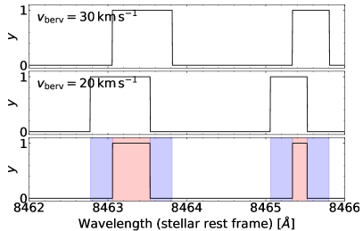
Figure 1: Example of template completion using a binary telluric mask. Upper and middle panels: Small section of the telluric binary mask for two observations after the correction for Earth’s barycentric motion. Wavelength ranges with $y=1$ are masked as tellurics. Lower panel: Resulting mask of the template. The red shaded wavelength ranges correspond to template knots with $M_{k}=0$ and contribute to the total masked template fraction $\gamma$. The blue shaded wavelength ranges are used for telluric modeling and contribute to $\gamma\,^{\prime}$.

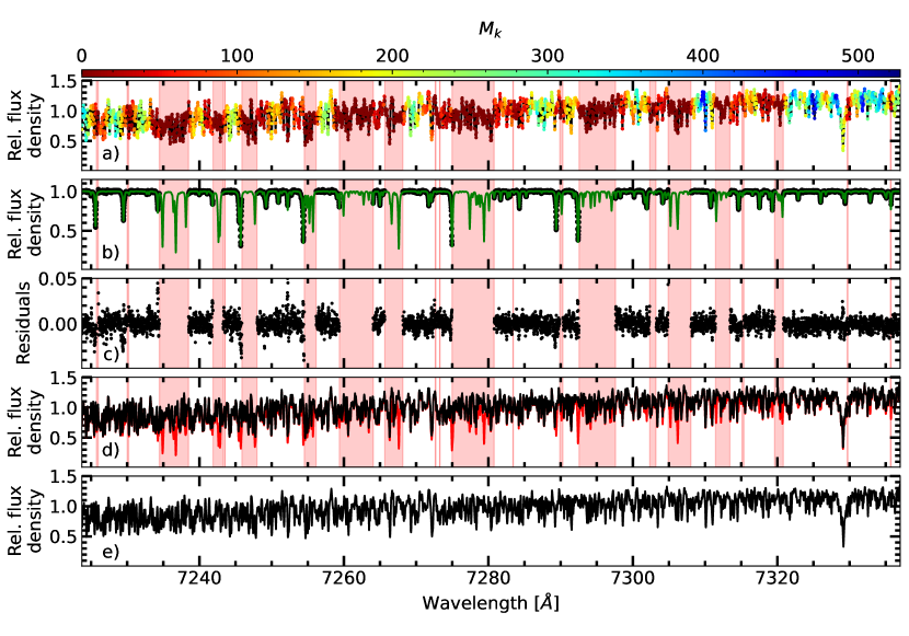
Figure 2: Illustration of the TDTM method. Panel a: Segment of the VIS template spectrum of Wolf 294. The number $M_{k}$ of exposure pixels that contribute to each template knot is color-coded. The red shaded wavelength ranges mark knots with $M_{k}=0$. Panel b: One residual telluric spectrum $F_{n,i}/S(\lambda_{n,i})$ (black dots) after the division of the science spectrum by the template, and the best-fit telluric model ($T(\lambda_{n,i})$, green line) derived with molecfit. The red shaded wavelength ranges are excluded from the transmission model fit. Panel c: Absolute residuals $F_{n,i}/S(\lambda_{n,i})-T(\lambda_{n,i})$ of the fit. Panel d: CARMENES spectrum before ($F_{n,i}$, red line) and after ($F_{n,i}/T(\lambda_{n,i})$) correction with the transmission model derived with molecfit (black line). Panel e: Telluric free high S/N template spectrum of Wolf 294 (black line) built using 444 telluric absorption-corrected CARMENES observations. The order has an S/N of 2310.

3.1 Template construction

We used the serval code (Zechmeister et al., 2018) to compute the stellar template spectrum based on a time series of input spectra. Following the nomenclature of Zechmeister et al. (2018), we indexed the set of spectra by $n=1,...,N$, and each spectrum was composed of discrete flux density measurements $f_{n,i}$ at pixel $i$ with uncertainties $\epsilon_{n,i}$ and calibrated wavelengths $\lambda_{n,i}$. We furthermore write the continuous model for the observation in the form

$$f(\lambda)=[s(\lambda)\cdot t(\lambda)]\otimes L(\lambda)\,,$$ (1)

where $s(\lambda)$ denotes the intrinsic stellar spectrum, $t(\lambda)$ the intrinsic telluric absorption spectrum at the time of observation, $L(\lambda)$ the LSF, and $\otimes$ the convolution operator.

In each observation, a stellar spectrum with an a priori unknown RV shift and a telluric spectrum with variable properties, but fixed in the rest frame of the Earth, were superimposed. The ultimate goal of serval is to derive precise measurements of the stellar RV. To this end, a preferably accurate and complete template of the stellar spectrum is required. This template was constructed by serval from the spectral time series, following an iterative and sequential forward-modeling approach.

Template completeness is improved by taking advantage of the relative RV shift of the stellar and telluric spectra induced by Earth’s barycentric motion, which can uncover sections of the stellar spectrum in some observations that may be affected by telluric lines in others with a less favorable relative RV shift. To identify these sections, serval uses a binary mask $m_{n,i}$, flagging spectral pixels that are affected by known atmospheric absorption features that are typically deeper than 1 % (see Sect. 3.2). Additionally, serval employs a bad-pixel map that flags saturated pixels, outliers, pixels providing unphysical (negative) flux densities, and pixels affected by sky emission. The template S/N is improved by coadding the individual spectra after an appropriate RV shift. During this process, the spectra are transformed to the stellar rest frame, that is, they are corrected for barycentric and stellar RVs. serval also accounts for secular acceleration, which is a change in the stellar radial velocity due to the high proper motion of close-by stars (Kürster et al., 2003; Zechmeister et al., 2009).

As a starting point for RV and template calculation, serval calculates preliminary RVs using the highest S/N spectrum of the CARMENES spectral time series as a template. These RVs are subsequently used to improve the stellar template spectrum by coadding the individual spectra and by obtaining higher precision RVs. This process is repeated until convergence is achieved. All masked pixels are excluded, and telluric-affected pixels are heavily downweighted in the process of coadding to isolate the stellar spectrum in the template.

The process of improving the template completeness by taking advantage of the relative shift of the mask is demonstrated in Fig. 1. The upper and middle panels show a segment of the telluric mask position of two observations after the correction for Earth’s barycentric motion. The lower panel shows the resulting mask of the template, assuming that the intrinsic RV shift of the stellar spectrum remained small. In the blue shaded regions, the stellar spectrum is shown in one of the observations, and only the red shaded ranges remain hidden. This results in an improvement of the template wavelength coverage.

Shifting the spectra to the same reference wavelength results in a wavelength sampling that differs for data taken at different nights. serval avoids resampling the spectral data on a new discrete wavelength grid and directly carries out a cubic B-spline regression. In essence, the template is the best-fitting spline through scattered data, and it is a continuous function that can be evaluated at any point within its boundaries, as illustrated in Fig. 2 of Zechmeister et al. (2018). The uniform cubic B-spline has equidistant knots $k$ on a logarithmic wavelength grid $\ln\lambda_{k}$. Typically, the number of template knots is comparable to the number of pixels per spectral order. In the following, $s_{k}=s(\lambda_{k})$ refers to the stellar template flux density at the knot positions. As an example, a section of the template of Wolf 294 is shown in Fig.2a.

As a crucial quantity for the TDTM approach, we define $M_{k}$ as the number of unflagged pixels that contribute to a knot. $M_{k}$ is stored for each template knot. The link between $M_{k}$ and the mask can be inferred from the lower panel of Fig. 1. In this specific example with only two observations, $M_{k}=0$ for template knots falling into the red marked wavelength range, $M_{k}=1$ for knots within the blue wavelength range, and $M_{k}=2$ for the remaining part of the spectrum.

Therefore, given one particular template knot $k$, three situations are possible: (1) all pixels contributing to this knot contain spectral information (i.e., are not masked), (2) all pixels are masked, (3) some pixels contain spectral information, while the remaining pixels are masked. The quantity $M_{k}$ is maximized in case (1), decreases for knots that are partly affected by tellurics in case (3), and takes a value of $M_{k}=0$ for pixels in case (2). For sampling reasons, spectra can contribute more than one pixel to a template knot, so that $M_{k}$ can exceed the number $N$ of observations. This is demonstrated in Fig. 2a, where a few template knots have $M_{k}\gtrsim 500$, although the number of observations is $N_{\rm VIS}=444$. The red shaded areas show wavelength ranges for which $M_{k}$ is zero, that is, the stellar spectrum could not be recovered.

As the total masked template fraction $\gamma$, we defined the fraction of masked ranges ($M_{k}=0$) compared to the entire wavelength range of the spectrum. As a result, the template completeness corresponds to $1-\gamma$ and depends on barycentric RV of the observer. The wavelength ranges of the stellar spectrum that are characterized by overlapping masked and nonmasked regions, indicated by the blue shaded areas in Fig. 1 and recovered in the process, are now additionally available for RV calculation and telluric modeling. We denote the total fraction of these ranges compared to the entire wavelength range of the spectrum by $\gamma\,^{\prime}$.

3.2 Mask construction

The telluric mask is an essential ingredient of the TDTM technique. As telluric features are ubiquitous, mask construction needs to balance strictness and achievable template completeness. While a restrictive mask that covers all relevant telluric features is crucial for creating a useful stellar template, an overly strict mask that declares extended chunks of the spectrum unusable jeopardizes the derivation of a template with any practical value.

To construct masks, we computed a synthetic telluric transmission model including H₂O, O₂, CO₂, and CH₄ using molecfit. As input parameters, we used the median observational and atmospheric parameters in the data set of each star and adopted the values from the standard atmosphere profile for the column densities of the atmospheric constituents. In the resulting transmission models, we normalized wavelength ranges that were affected by molecular continuum absorption. For each target, we finally computed a binary mask by flagging all model features that were deeper than a specified threshold. In our analysis, we found that thresholds of $\sim 1\,\%$ provide a reasonable compromise between capturing the vast majority of telluric features and removing critical portions of usable spectrum.

3.3 Extraction of the telluric spectrum

To extract the telluric transmission spectrum, we wish to remove the stellar contribution from the individual observations by division. Following Vacca et al. (2003), we therefore approximated the convolution of the product in Eq. (1) by

$$F(\lambda) \approx[s(\lambda)\otimes L(\lambda)]\cdot[t(\lambda)\otimes L(\lambda)]$$ (2)

$$=S(\lambda)\cdot T(\lambda)\,,$$ (3)

which is now a product of the convolved intrinsic stellar flux density and the convolved telluric spectrum,

$$S(\lambda) =s(\lambda^{\prime})\otimes L(\lambda,\lambda^{\prime})$$ (4)

$$T(\lambda) =t(\lambda^{\prime})\otimes L(\lambda,\lambda^{\prime}).$$ (5)

We discuss the validity of this approximation in Appendix A.

Dividing the observed spectra by the appropriately shifted template, we derived a residual spectrum that is essentially free of stellar features,

$$\frac{F_{n,i}}{S(\lambda_{n,i})}\approx T(\lambda_{n,i})\;.$$ (6)

As the uncertainty of the template is typically negligible compared to that of the individual observations as $M_{k}\gg 1$, we did not propagate the template uncertainty and used the uncertainty of the observed spectra in the modeling of the individual residual spectra.

The residual telluric transmission spectrum of Wolf 294 is shown in Fig. 2b. Again, the red bands represent template knots for which the residual spectrum could not be constrained. Consequently, these sections are not used to model the telluric lines.

3.4 Modeling the telluric lines

Table 1: molecfit fitting ranges used to calibrate the models for CARMENES VIS and NIR spectra.

Channel	$\Delta\lambda$ [Å]	Main absorber
VIS	5375–5530	H2O
VIS	5650–6040	H2O
VIS	6260–6620	O2, H2O
VIS	6860–7450	O2, H2O
VIS	7590–7740	O2
VIS	7830–8600	H2O
VIS	8800–9270	H2O
NIR	9750–10 350	H2O
NIR	10 600–11 000	H2O
NIR	11 600–12 400	H2O
NIR	12 400–13 100	O2
NIR	15 110–15 400	H2O
NIR	15 600–15 800	CO2
NIR	15 900–16 200	CO2
NIR	16 350–16 660	CH4
NIR	16 850–17 100	CH4, H2O

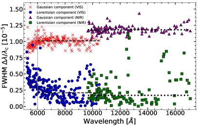
Figure 3: Measured Gaussian and Lorentzian FWHM components of hollow cathode emission lines as a function of wavelength for the VIS and NIR CARMENES spectrographs. The vertical gray line marks the cutoff wavelength at 6000 Å. The horizontal lines indicate median values of the Gaussian and Lorentzian FWHM components for the VIS (dashed lines) and NIR channel (dotted lines).

Table 2: Median averaged Gaussian and Lorentzian FWHMs.

Channel	Number	$w_{\mathrm{Gauss}}$	$w_{\mathrm{Lorentz}}$
	of lines	$[10^{-5}\Delta\lambda/\lambda_{c}]$	$[10^{-5}\Delta\lambda/\lambda_{c}]$
VIS	218	$1.00$	$0.28$
VIS ($>6000\,$Å)	159	$1.01$	$0.21$
NIR	114	$1.18$	$0.17$

The residual telluric spectrum was modeled using the molecfit package version 1.5.9 (Smette et al., 2015; Kausch et al., 2015) and the version 3.6 of the aer molecular line list. The altitude stratification of temperature, pressure, and molecular abundances served as input for LBLRTM. To create this profile, molecfit merges information from three sources: (1) a reference atmospheric profile, (2) global data assimilation system (GDAS) profiles, and (3) measurements of the ambient conditions obtained during the time of observations. In this study, we used a nightly midlatitude (45 deg) reference model atmosphere as the reference profile. In addition to the pressure and temperature distribution up to an altitude of 120 km as a function of height on a 1 km grid, the profile also provides the abundances of 30 molecules. The GDAS profiles describe the pressure, temperature, and relative humidity as a function of 23 altitude levels up to roughly 26 km.

In the spectral modeling with molecfit, we freely varied the abundances of O₂, CO₂, CH₄, and the atmospheric water vapor content. We carried out the model fitting over broad wavelength ranges that covered large portions of the molecular bands, taking full advantage of numerous unsaturated telluric lines contained in the CARMENES VIS and NIR channels; the selected fitting intervals are given in Table 1. In the modeling, the continuum level within the fitting ranges was approximated with a low-order polynomial. Since small errors in the wavelength calibration result in large residuals in the corrected spectra, we also allowed a Doppler shift of the transmission model to match the observed spectrum. In this way, instrumental drifts can be accounted for in the modeling. Wavelength ranges for which no stellar template was available ($M_{k}=0$) were excluded from the fit, along with sections affected by sky emission features.

molecfit requires the instrumental LSF in the modeling. In the case of CARMENES, the LSF can be represented by a combination of two profiles, one Gaussian and one Lorentzian. We performed an extensive analysis to derive appropriate parameters for the LSFs of the two CARMENES channels based on calibration data (see Sect. 3.5). Therefore, the parameters of the LSF were not free in the modeling.

3.5 CARMENES instrumental line profile

For a proper modeling of the telluric lines, the LSF needs to be well known. In order to characterize the LSF, we analyzed hollow cathode lamp spectra taken for the purpose of calibration before and after the science observations.

An accurate estimation of the line shape is not trivial because the lines are sparsely sampled. Within each échelle order, the coverage of the full width at half maximum (FWHM) of the LSF typically increases from about 2.5 to 4.0 pixels along the main dispersion direction from the blue to the red part of the order. Due to several instrumental effects (e.g., temperature variations), the spectra move across the detector with time. We therefore combined multiple exposures to artificially increase the sampling. A total of 1455 different lamp exposures in the VIS channel and 2605 in the NIR channel were used for this purpose. For each line we investigated in that manner ($218$ in the VIS and $114$ in the NIR), the frames were aligned so that the line was centered. Before they were combined, they were normalized.

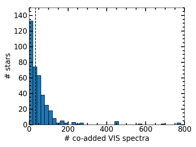
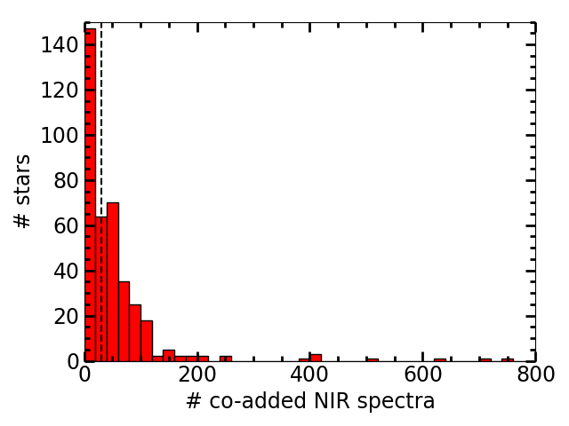
Figure 4: Distribution of the number of telluric-corrected spectra we used to build the templates for all sample stars in the VIS (left) and NIR (right). The vertical dashed lines indicate the median values at 34 in the VIS and 30 in the NIR.

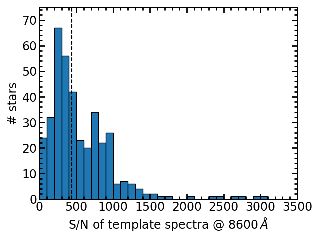
Figure 5: Distribution of the S/N of a reference order for the VIS (order 70 around 8 600 Å, left) and the NIR (order 52 around 10 500 Å, right). The vertical dashed lines indicate the median values at 438 in the VIS and 482 in the NIR.

These superimposed line profiles are well suited to modeling the shape of the LSF. For this purpose, we tested different profiles, namely Gaussians and Lorentzians, generalized Gaussians and Lorentzians with the exponent treated as an additional free parameter, as well as Voigt profiles, which are defined by the convolution of Lorentzian and Gaussian distributions. The analysis of all fits showed that a Voigt profile is the most appropriate for the LSF modeling. The other profiles were usually not suitable for a proper simultaneous handling of the line cores and lobes.

In addition, we investigated the variations in the measured line widths, $\Delta\lambda$, across the detector and found that except for some secondary but significant features near the detector edges (particularly in the blue part of the VIS CCD), the line widths still can be described in a consistent manner. The dominant effect becomes apparent when the widths of the lines are expressed in terms of wavelength. In the Voigt profile, the overall width can be described by its Gaussian and Lorentzian components. If the resolution remains constant, both components should exhibit a linear trend in wavelength. However, when they are represented in wavelength-independent units using $\Delta\lambda/\lambda_{c}$, where $\lambda_{c}$ represents the central vacuum wavelength of the specific line, these normalized widths are expected to stay constant if the spectrograph resolution is independent of wavelength.

In Fig. 3 we show the measured Gaussian and Lorentzian FWHM components of the Voigt profile for both channels. The NIR channel has a somewhat lower resolution and therefore presents a wider Gaussian component than the VIS channel. However, the widths of the Lorentzian component are very similar for both channels redward of 6000 Å.

To obtain robust estimates of the LSF parameters, we used medians for the FWHM of each component and channel to model the instrumental LSF of CARMENES. These parameters are summarized in Table 2. Due to the clearly visible deviation in the blue part of the visual channel, we considered only lines with a wavelength above 6000 Å. Moreover, the distribution of the Lorentzian component, particularly in the NIR part of the spectrum, shows some conspicuous features. Some outliers cluster around $12\,500$ Å, while the scatter seems generally increased for wavelengths above 15 000 Å. The reasons for these effects could not consistently and objectively be traced back to line blends or similar effects.

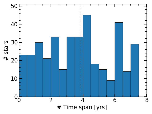
Figure 6: Time-span distribution of the observations for the sample stars for the VIS (left) and NIR spectra (right). The vertical dashed lines indicate the median values at $3.83$ years in the VIS and $3.70$ years in the NIR.

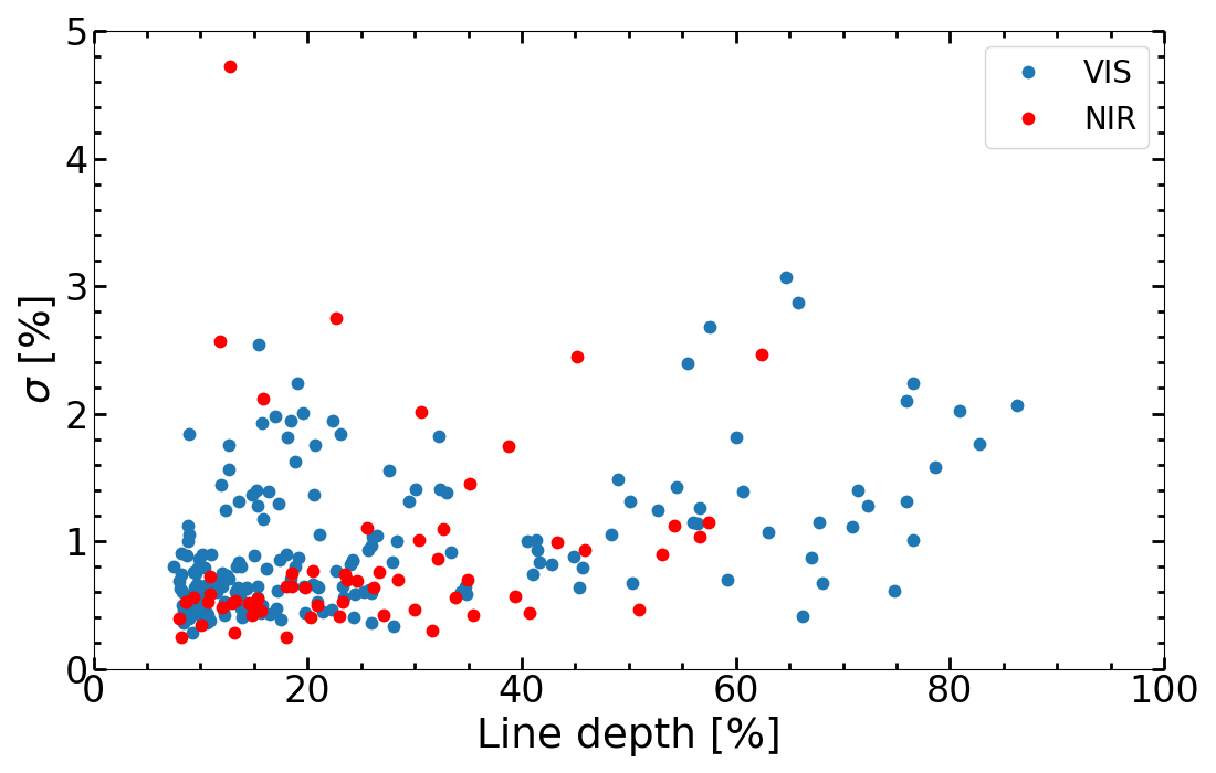
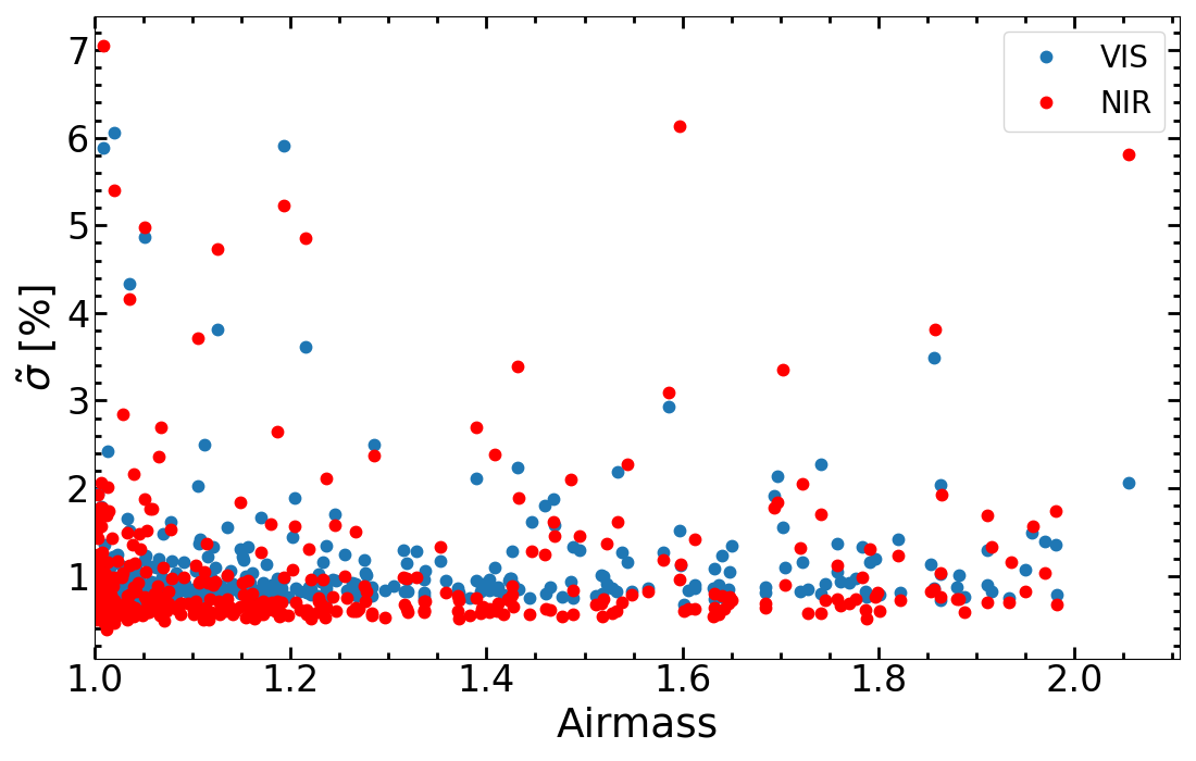
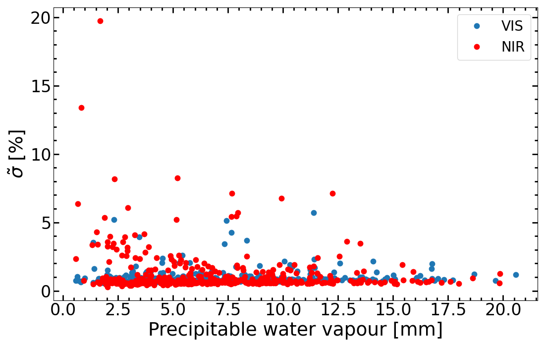
Figure 7: Metrics for assessing the quality of the telluric correction. Top panel: Residual standard deviation ($\sigma$) vs. line depth for a single Wolf 294 VIS (blue) and NIR (red) spectrum. Middle panel: Median residual standard deviation ($\tilde{\sigma}$) vs. airmass for all Wolf 294 VIS and NIR spectra. Bottom panel: Median $\tilde{\sigma}$ for telluric water bands vs. precipitable water vapor for all Wolf 294 VIS and NIR spectra.

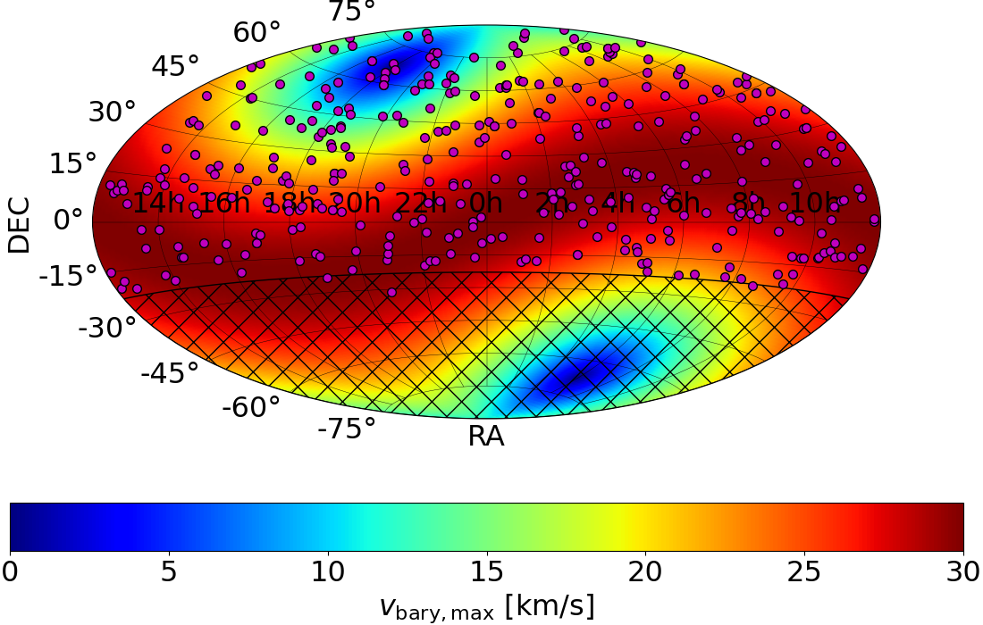
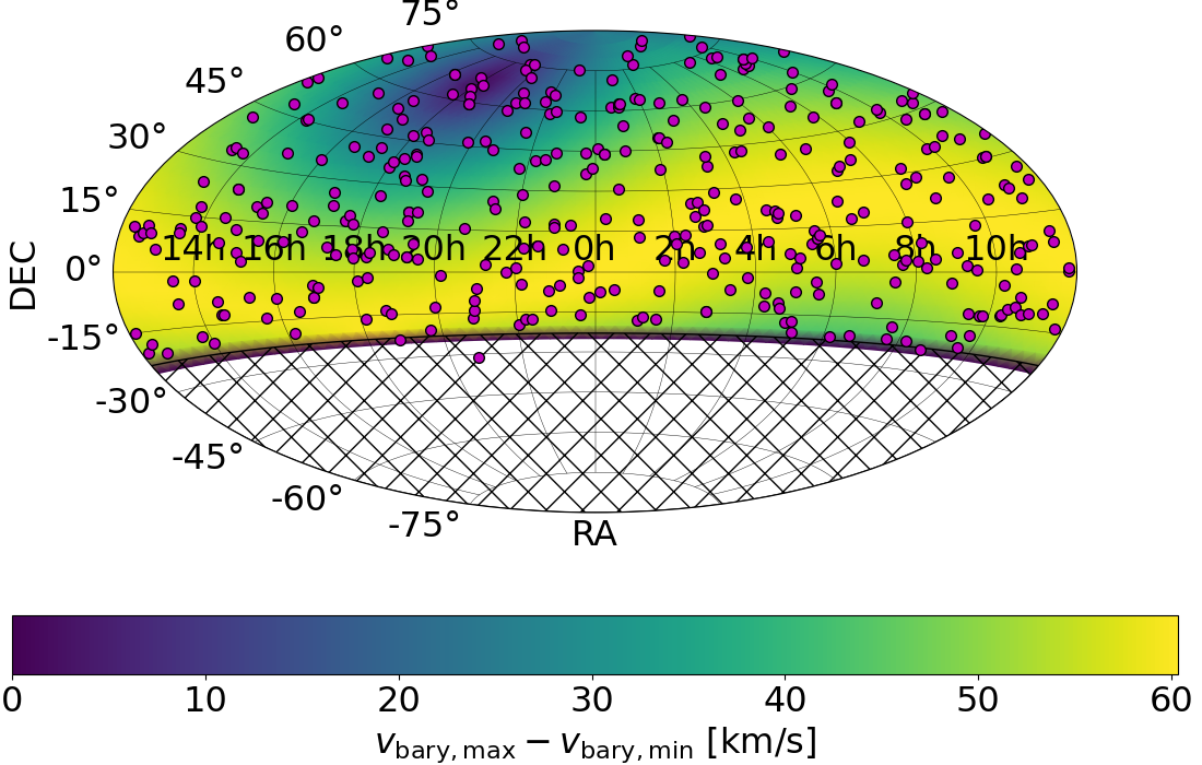
Figure 8: Sky maps in Aitoff projection of the maximum absolute barycentric RV $\varv_{\rm bary,\,max}$ as derived from Eq. (10) (left panel) and full amplitude of the barycentric RV $\varv_{\rm bary,\,max}-\varv_{\rm bary,\,min}$ (right panel) for nights when the star is observable above 30 deg over the horizon for the location of the Calar Alto Observatory. The positions of the 382 sample stars (purple circles) are indicated. The hatching pattern indicates the visibility cutoff at $\delta<-23$ deg of the CARMENES sample.

3.6 Removing the telluric lines

After fitting a transmission model to the residual telluric spectrum with molecfit, we used the best-fit parameters as input to compute a synthetic transmission model over the entire wavelength range of the observation with the calctrans module of molecfit. To derive the spectrum corrected for telluric lines $\hat{F}_{n,i}$, we finally divided the CARMENES observation by the transmission model $T(\lambda_{n,i})$,

$$\hat{F}_{n,i}=\frac{F_{n,i}}{T(\lambda_{n,i})}\;.$$ (7)

As an example, we show one observed and its telluric corrected spectrum of Wolf 294 in Fig. 2d.

4 Telluric-corrected M-dwarf template library

4.1 Sample overview

We applied the TDTM method to each of the 382 targets in our sample and generated a spectrum corrected for telluric absorption for each individual VIS and NIR CARMENES observation. The telluric-corrected spectra for each target were subsequently coadded to create a telluric-free stellar template spectrum with a high S/N with serval. We show the example of Wolf 294 in Fig. 2e, where the displayed order reaches a S/N of 2310.

To construct the library of telluric-free template spectra with a high S/N, we used a total of 22 357 VIS and 20 314 NIR observations obtained between 2016 and 2023 that were telluric-corrected with the TDTM method before coaddition. In Table 3 we present the sample of stars we used in this study and provide information on the targets. In particular, we tabulate the CARMENES identifiers, common names, Gliese-Jahreiss numbers, equatorial coordinates at epoch J2000, spectral types, 2MASS $J$ magnitudes (Alonso-Floriano et al., 2015; Caballero et al., 2016a), the number of telluric-corrected VIS and NIR spectra used to create the telluric-free stellar templates, and the estimated S/N of a reference order at 8 600 Å for the VIS templates and at 10 500 Å for the NIR templates. Our template spectra can be downloaded from the CARMENES GTO Data Archive (Caballero et al., 2016b).

In the VIS, the number of spectra used for the coadding ranged from 5 up to 774, with a very similar number of spectra in the NIR (from 4 to 756). In the reference orders, the range of the S/N in the VIS varies between 9 and 3057, and in the NIR, it varies between 9 and 3270. We show the distributions of the number of spectra we used for the coaddition in Fig. 4. The median values indicated by the vertical dashed lines in both figures are 34 in the VIS and 30 in the NIR. The distributions of the S/N of the template spectra given in the reference orders are shown in Fig. 5, with median values of 438 in the VIS and 482 in the NIR. Finally, we present the time span of the observations covered for each target in Fig. 6, with median values of 3.83 years in the VIS and 3.70 in the NIR.

4.2 Correction accuracy

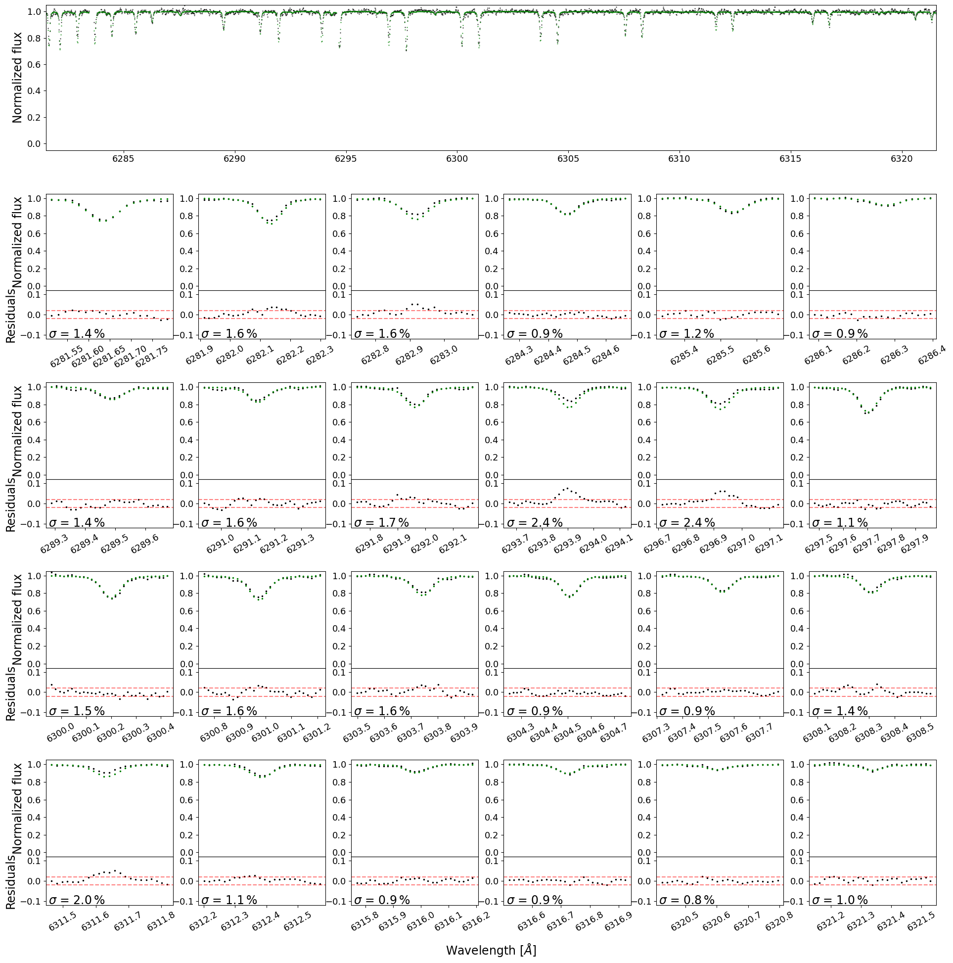
Figure 12: Example of telluric line fits for the O₂ band in a single Wolf 294 spectrum. The top panel displays the residual telluric spectrum (black dots) after dividing the science spectrum by the stellar template, and the best-fit telluric model (green dots) derived with molecfit. The subplots illustrate the individual telluric lines (top) and the residuals (bottom, black dots), with dashed red lines marking a $2\,\%$ deviation between data and model. The standard deviation $\sigma$ of the residuals is also shown in each subplot.

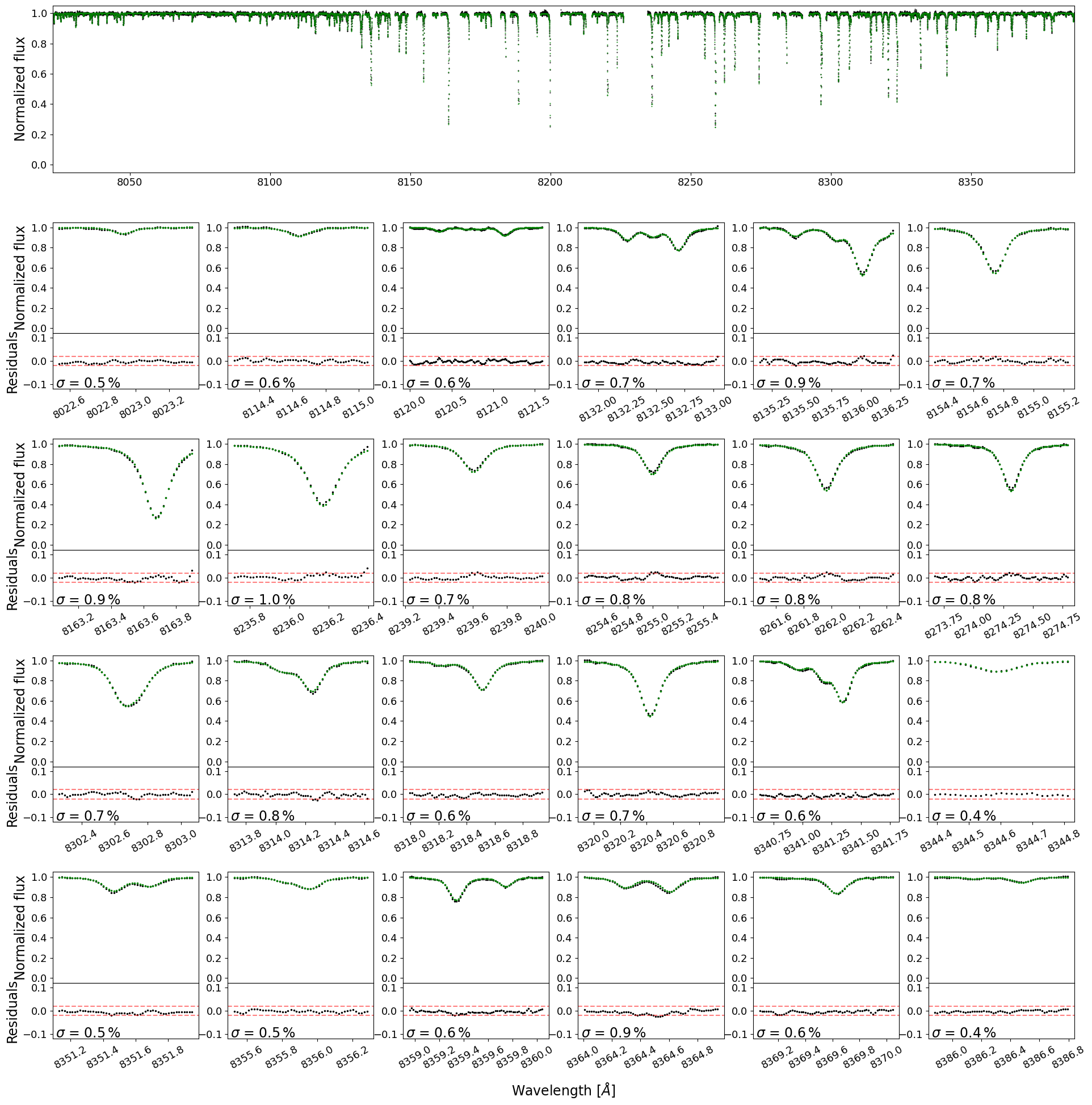
Figure 13: Same as Fig. 12, but for the H₂O band around $8\,200\,$Å.

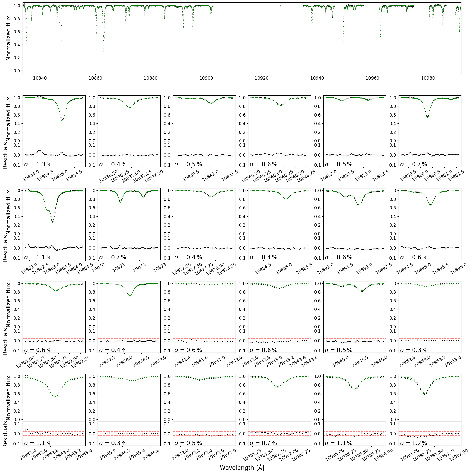
Figure 14: Same as Fig. 12, but for a H₂O band around $11\,000\,$Å.

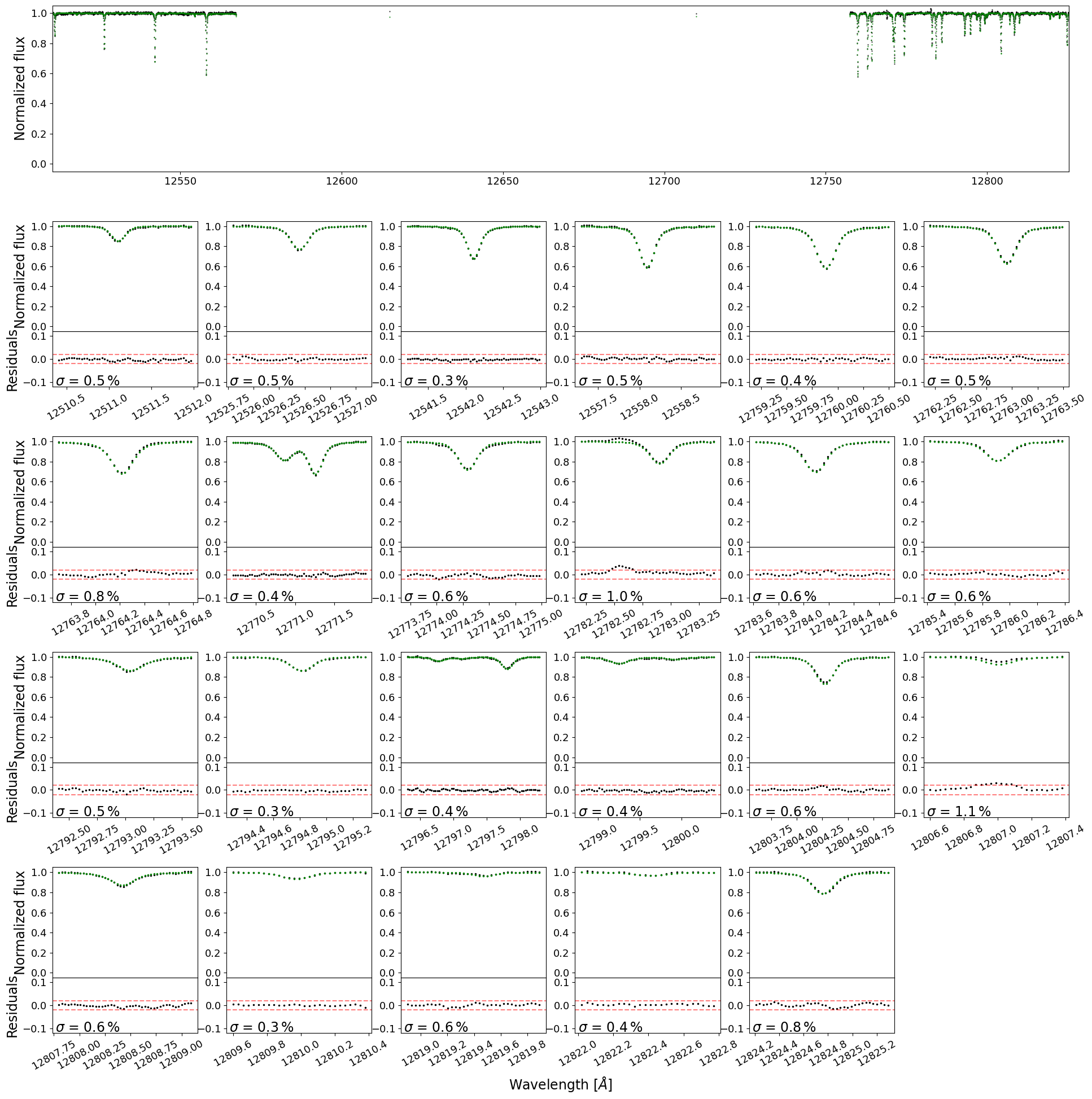
Figure 15: Same as Fig. 12, but for a O₂ band around $12\,600\,$Å.

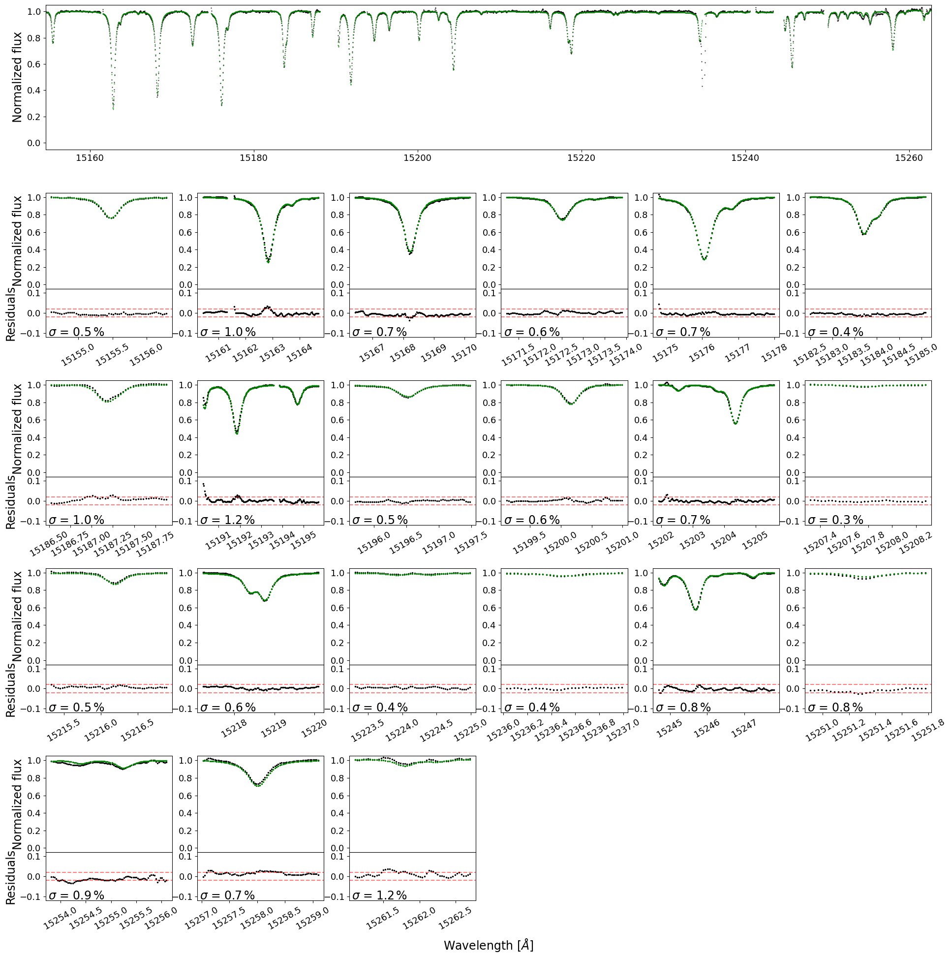
Figure 16: Same as Fig. 12, but for a H₂O band around $15\,000\,$Å.

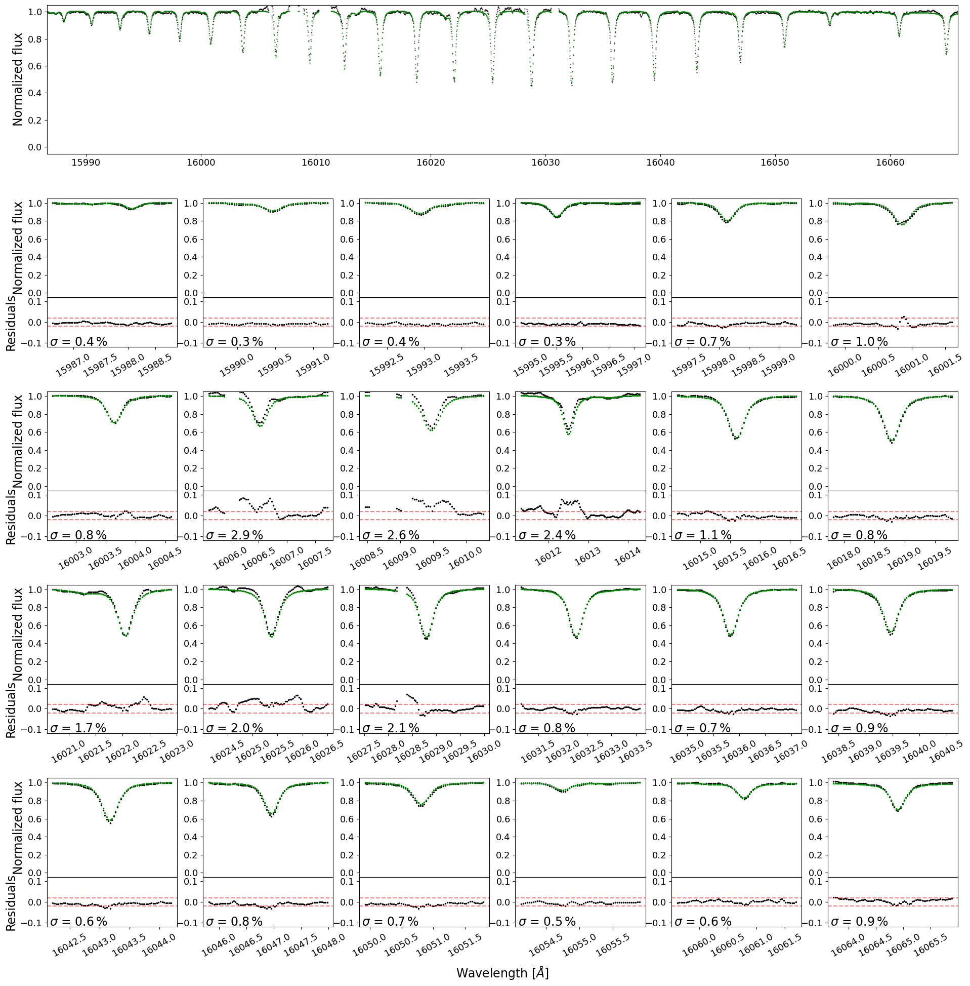
Figure 17: Same as Fig. 12, but for a CO₂ band around $15\,800\,$Å.

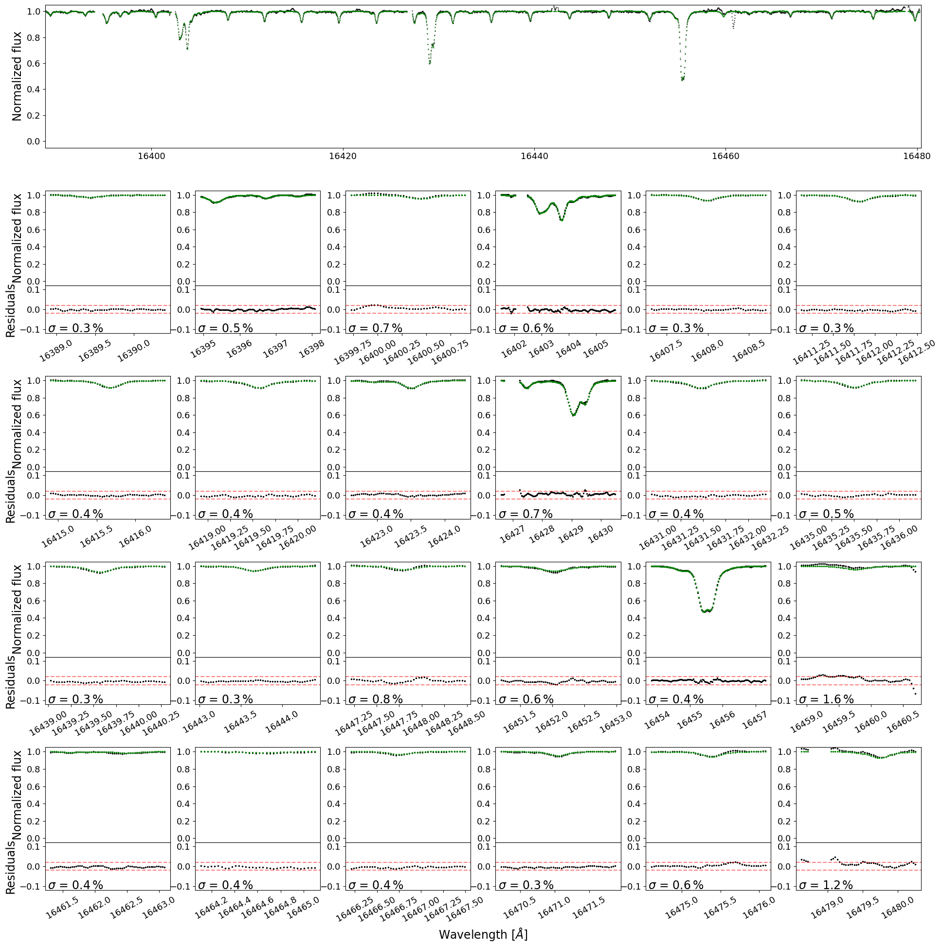
Figure 18: Same as Fig. 12, but for a CH₄ band around $16\,400\,$Å.

In the following, we examine the accuracy of the telluric correction applied to individual VIS and NIR CARMENES spectra of Wolf 294, using the TDTM approach. Figures 12-18 display examples of the corrections applied to individual lines within a single spectrum, with a focus on specific molecular constituents. For VIS, these molecules include O₂ and H₂O, while in NIR, they extend to O₂, H₂O, CO₂, and CH₄. We assessed the accuracy of these corrections by computing the standard deviation $\sigma$ of the residuals. In most cases, $\sigma$ was found to be below the 1 % level. An exception was observed in the O₂ lines within the VIS spectrum, which generally fell within the 1–2 % range. Additionally, some CO₂ lines exhibited $\sigma$ values greater than 2 %. These discrepancies may be attributed to an inadequate removal of the stellar spectrum, leading to a distortion in the telluric residual spectrum in the given instance.

To further analyze the variability in the residuals relative to the line depth, an automated procedure was implemented. This procedure detected lines in the telluric residual spectrum, fit a Gaussian model to ascertain the depths, positions ($\mu$), and widths ($\sigma_{\rm Gaussian}$) of the telluric lines, and measured the variability in the residuals within a wavelength range of $\mu\pm 3\,\sigma_{\rm Gaussian}$. The top panel of Fig. 7 illustrates the results for a single spectrum of Wolf 294. In both CARMENES channels, the $\sigma$ values were confined to a range of 0.3 to 3.0 %. Optimal outcomes were observed for line depths up to 30 %, where $\sigma$ was mostly lower than 1 %. Our findings indicated a weak or nonexistent correlation between $\sigma$ and line depth.

Subsequently, we explored the variability in the residuals as a function of airmass for all VIS and NIR spectra of Wolf 294. To this end, we introduced $\tilde{\sigma}$, defined as the median of the measured $\sigma$ values within a single Wolf 294 spectrum, and we present the results in the middle panel of Fig. 7. Most spectra exhibited a $\tilde{\sigma}$ value of approximately 1–2 % in the entire airmass range. The discrepancy in $\tilde{\sigma}$ between the VIS and NIR channels is ascribed to the reduced number of usable telluric lines in the NIR spectra relative to the VIS spectra (see the top panel of Fig. 7), leading to reduced scatter and, consequently, a lower value for $\tilde{\sigma}$. However, a minor subset of spectra revealed $\tilde{\sigma}$ values that reached up to 6–7 %. A visual inspection identified these spectra as characterized by low S/N.

Finally, we calculated $\tilde{\sigma}$ and only included H₂O telluric lines. We display the results as a function of precipitable water vapor derived with molecfit, as illustrated in the bottom panel of Fig. 7. Although the $\tilde{\sigma}$ values derived in the NIR exhibit greater scatter than the VIS spectra, the findings in both channels agree and did not disclose any discernible trends.

Overall, our results indicate that the correction accuracy mostly depends on the S/N of the data and to a much lesser extent on the depth of the telluric features. Most telluric features can be corrected to basically within the noise level. Deep lines are problematic for two reasons. First, the S/N decreases in their cores, and second, lines deeper than $50\,\%$ can leave comparatively large systematic residuals in the corrected spectra, especially in the line cores. These residuals may be attributed to the fact that small discrepancies between model and observation can result in large residuals, especially in deep lines. These discrepancies may result from uncertainties in the line strengths listed in the HITRAN database, leading to inaccurate column density fits (Seifahrt et al., 2010; Gordon et al., 2011). Potential uncertainties in the line positions affect the wavelength calibration, causing P Cygni-like residuals in the worst cases. Incomplete corrections may also arise from the instrumental line profile model. The Gaussian and Lorentzian profile parameters from different lines show some scatter and are approximated by a constant value (see Sect. 3.5). Another source of uncertainty is the approximation of Eq. (1) by Eq. (3), which becomes particularly relevant for blends between telluric and stellar lines (Sameshima et al., 2018, their Appendix A).

We find that most telluric absorption features are corrected to within 2 % or better of the continuum standard deviation, as reported by Smette et al. (2015). For objects with numerous intrinsic features, the authors proposed to apply molecfit to TSSs observations taken with the same instrumental setup as the science object to solve for the polynomial continuum coefficients. These results are then used as fixed input to subsequently apply molecfit for the science observation’s telluric correction. Our approach, however, is able to accurately and directly extract telluric features of various strengths for wavelength ranges with $M_{k}>0$, even for feature-rich objects such as M dwarfs, whose spectra are dominated by numerous molecular features in the VIS and NIR bands.

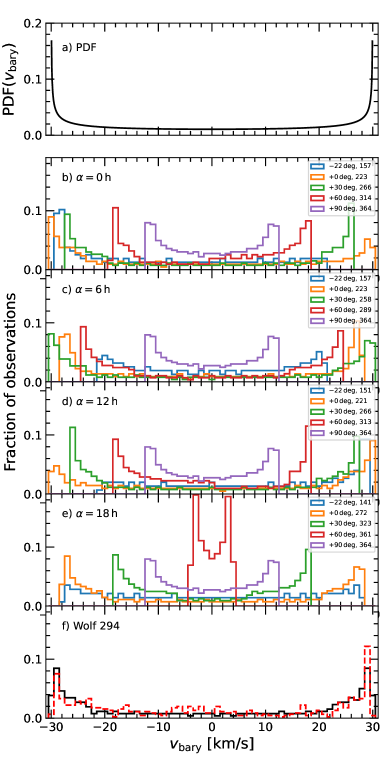
Figure 9: Barycentric velocity distributions corresponding to various coordinate sets. Panel a: Probability density function $\mathrm{PDF}(\varv_{\rm bary})$ as computed with Eq. (13). Panels b-e: Simulated barycentric velocity distributions for targets with $\alpha=0\,$h, 6 h, 12 h, and 18 h, and $\delta=-22\,{\rm deg},0\,{\rm deg},+30\,{\rm deg},+60\,{\rm deg},+90\,{\rm deg}$, assuming one daily measurement over a time span of one year and considering the target visibility. The second entry in the legend is the number of total observing nights. Panel f: Simulated barycentric velocity distribution of Wolf 294 (black line). The barycentric velocity distribution for the datasets of Wolf 294 (dashed red line) is overplotted.

4.3 Visibility constraints

For the TDTM technique to work properly, a good template is essential. While a lack of S/N may be addressed by taking more observations, which may pose a practical but not a fundamental problem, the relative shift between telluric and stellar lines is also crucial for the template construction. In the case of planet-induced reflex motion, the barycentric motion of the Earth and its rotation dominate the sum of relative shifts. The maximum absolute barycentric velocity $\varv_{\rm bary,\,max}$ depends on the ecliptic latitude $\beta$ of a target,

$$\varv_{\rm bary,\,max}\approx 30\,\mathrm{km\,s}^{-1}|\cos\beta|\;.$$ (8)

The transformation from the ecliptic $(\lambda,\beta)$ to the equatorial system $(\alpha,\delta)$ with the axial tilt of the Earth $\varepsilon\approx 23.44$ deg yields

$$\sin\beta=\sin\delta\cos\varepsilon-\cos\delta\sin\alpha\sin\varepsilon\,.$$ (9)

Thus, $\varv_{\rm bary,\,max}$ as a function of $\alpha$ and $\delta$ reads

$$\varv_{\rm bary,\,max}(\alpha,\delta)\approx 30\,\mathrm{km\,s}^{-1}\sqrt{1-\sin^{2}\beta(\alpha,\delta)}\,,$$ (10)

which provides a sky map as in the left panel of Fig. 8 showing the maximum offset between telluric lines and stellar lines. Except for objects situated near the ecliptic poles, $\varv_{\rm bary,\,max}$ is larger than the natural line width of the tellurics and the instrumental resolution ($\sim 3\,$km s^-1), which is required to disentangle the stellar and telluric spectra.

To examine the largest possible improvement on the template completeness, we carried out a simulation of the full amplitude of the barycentric velocity range $\varv_{\rm bary,\,max}-\varv_{\rm bary,\,min}$ as a function of ecliptic coordinates down to the visibility cutoff for stars with $\delta<23$ deg, which is also the CARMENES survey limit (Garcia-Piquer et al., 2017). In particular, we computed the dates on which a target is 30 deg above the horizon between the astronomical dusk and dawn for the location of the Calar Alto Observatory, and calculated the barycentric RV at midnight for these dates. In the right panel of Fig. 8, we show the difference between the maximum and minimum barycentric RV $\varv_{\rm bary,\,max}-\varv_{\rm bary,\,min}$ for each pair of coordinates.

The observed barycentric velocity range is further constrained by the visibility. The main contribution to the barycentric velocity is a yearly sinusoid. We considered an object with a half-year visibility period, during which the barycentric Earth RV changes from a maximum to a minimum. In particular, we considered the first half of a cosine

$$\varv_{\rm bary}(t)=\varv_{\rm bary,\,max}\cdot\cos\left(\frac{2\pi t}{T_{\oplus}}\right)\;,$$ (11)

where $T_{\oplus}$ is the orbital period of the Earth. When the target is observed at a random time, the probability to observe a barycentric RV shift equal to or smaller than $\varv_{\rm obs}$ is

$$P(\varv_{\rm bary}\leq\varv_{\rm obs})=1-\frac{1}{\pi}\arccos\left(\frac{\varv_{\rm obs}}{\varv_{\rm bary,\,max}}\right)\;.$$ (12)

The probability density function, $\mathrm{PDF}(\varv_{\rm bary})$, to observe the target in some interval of barycentric velocity is given by

$$\mathrm{PDF}(\varv_{\rm bary})=\frac{1}{\pi\;\varv_{\rm bary,\,max}\sqrt{1-\left(\frac{\varv_{\rm bary}}{\varv_{\rm bary,\,max}}\right)^{2}}}\;,$$ (13)

which is shown in Fig. 9a.

To study the barycentric velocity distribution as a function of right ascension and declination over one year for the location of the Calar Alto Observatory, we carried out simulations for a set of coordinates with $\alpha=0\,$h, 6 h, 12 h, and 18 h, and $\delta=0\,{\rm deg},+30\,{\rm deg},+60\,{\rm deg}$, and $+90\,{\rm deg}$. In addition, we included a southern coordinate sample with $\delta=-22$ deg, which is near the visibility limit of the CARMENES survey. Assuming that objects can generally only be observed down to an elevation of $30$ deg, we determined the nights when the target is observable and computed the barycentric velocity at the time between evening and morning astronomical twilight. Our results are presented in Fig. 9b-e. The simulated distributions show a plateau around $\varv_{\rm bary}=0$ and increasing slopes at both ends where $\varv_{\rm bary}\rightarrow\pm\varv_{\rm bary,\,max}$. This shape is a consequence of the regular sampling of the yearly sinusoidal barycentric velocity contribution. However, the simulations show that all barycentric velocities between $-\varv_{\rm berv,\,max}$ and $+\varv_{\rm berv,\,max}$ are covered. We finally present the predicted and observed barycentric velocity distribution of Wolf 294 (Fig. 9f) of our spectroscopic data set.

4.4 Total masking fraction

In the case of Wolf 294, a mask that flags telluric features deeper than 1 % results in a total masking fraction $\gamma_{\rm max,\,VIS}=33.5\,\%$ for the optical spectral range (0.52–0.96 $\mu$m) and $\gamma_{\rm max,\,NIR}=62.8\,\%$ for the NIR (0.96–1.71 $\mu$m) when using one observation. As the number of observations with different barycentric velocities is increased, the total masked fraction decreases and converges to a limit of $\gamma_{\rm min,VIS}=16.5\,\%$ and $\gamma_{\rm min,NIR}=42.5\,\%$ for the 1 % mask. These limits are mainly defined by broad telluric features, for example, the strong water bands centered around 1.15 $\mu$m and 1.4 $\mu$m, which prevent further reduction of masked regions.

The difference between the maximum and minimum masking fraction is the total fraction that is gained for the modeling of the telluric spectrum, which is $\gamma\,^{\prime}_{\rm max,VIS}=17.0\,\%$ in the optical and $\gamma\,^{\prime}_{\rm max,NIR}=20.3\,\%$ in the NIR employing the 1 % mask. In the VIS, the useable amount of the stellar spectrum was increased from 66.5 % to 83.5 %, which corresponds to an increase of 25.6 %. The increment is even larger in the NIR, where the useable range was increased from 37.2 % to 57.5 %, which corresponds to a relative growth of 54.6 %.

We show the evolution of the total masked fraction using the 1 % mask for Wolf 294 Fig. 10. To reach the lower limit of the total masked fraction, it is necessary to cover the full range of barycentric velocities. As shown in Fig. 10, this requirement was fulfilled for Wolf 294 after the first observing season. Additionally, a limited number of observations at approximately $\pm 30\,$km s^-1 substantially reduces the total masked fraction. Our simulations indicate that with six observations that are uniformly distributed across the barycentric velocity space of $\pm 30$ km s^-1, values of 17.9 % in the VIS and 40.3 % in the NIR can be achieved. However, for proper telluric correction, a barycentric velocity coverage 2-5 times larger than the minimum 3 km s^-1 required to resolve the lines is essential, which means that velocity spans of 6–15 km s^-1 are imperative.

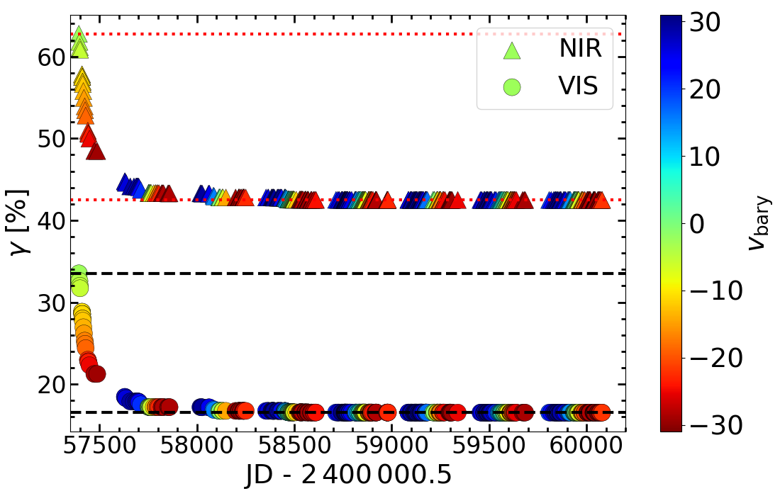
Figure 10: Evolution of the total masked wavelength fraction color-coded with the barycentric velocity for Wolf 294. The circles represent the VIS channel (bottom) and the triangles the NIR channel (top). The upper and lower dashed black lines mark the maximum and minimum limits of the total masked fraction in the optical wavelength range. The dotted red lines mark the same limits for the NIR wavelength range.

5 Summary and conclusions

We presented the TDTM technique, a combination of data-driven (template construction) and forward-modeling (spectral fitting) methods to correct for telluric absorption lines in high-resolution VIS and NIR spectra. After applying a telluric mask to a time series of spectra, we constructed a stellar template with a high S/N and used it to remove the stellar contribution from the observations. We then used molecfit to fit an atmospheric transmission model to the resulting telluric spectrum and finally corrected the target spectrum at all wavelengths. While the telluric correction via spectral modeling with molecfit alone is especially challenging for late-type stars with their high density of molecular lines, the TDTM technique is applicable to spectra of any spectral type. Although we chose the molecfit code to fit the transmission model to the telluric spectra in this work, other software packages that produce synthetic atmospheric transmission spectra, such as TelFit (Gullikson et al., 2014) or TAPAS (Bertaux et al., 2014), could be used.

Telluric correction with our method works best with a high number of observations and good coverage of the barycentric velocity space. To demonstrate the performance of our correction method, we applied it to high-resolution optical and NIR CARMENES observations of the M3.0 V star Wolf 294. We found that molecfit corrects most telluric lines close to noise level in the residual telluric transmission spectrum obtained with the help of the template. Moreover, we did not find a correlation between the correction accuracy and the depth of telluric lines.

We applied the TDTM approach to the whole CARMENES survey sample, which comprises 382 M-dwarf stars. After correcting for telluric lines, we coadded the individual observations and constructed telluric-corrected high-resolution template spectra with a high S/N for each of our targets. Our spectral library is publicly available and can be found on the CARMENES data archive homepage.

Appendix A Approximation of the convolution equation

In an actual observation, the product of the stellar spectrum, $s(\lambda)$, and the telluric transmission spectrum, $t(\lambda)$, is received by the system of telescope and spectrograph, which we call the instrument. The effect of the instrument on the received spectrum is modeled by a convolution with the instrumental LSF, $L(\lambda)$, so that we obtain the left-hand side of the equation,

$$[s(\lambda)\cdot t(\lambda)]\otimes L(\lambda)\approx[s(\lambda)\otimes L(\lambda)]\cdot[t(\lambda)\otimes L(\lambda)]\;.$$ (14)

As the convolution cannot easily be inverted, the left-hand side of Eq. (14) is frequently approximated as a product of two spectra separately convolved with the LSF. As previously pointed out, for instance, by Sameshima et al. (2018), the two sides of the equation differ. In their analysis, Sameshima et al. (2018) found that a telluric-corrected spectrum based on this approximation differs noticeably from the stellar spectrum if the width of the stellar lines is comparable to or narrower than the instrumental resolution and if the stellar lines are heavily blended with telluric features.

We analytically investigated the difference between the two sides of Eq. (14), making the simplifying assumption of normality for the stellar, telluric, and instrumental line profiles. In particular, we adopted

$$s(\lambda) = \frac{A_{s}}{\sqrt{2\pi\sigma_{s}^{2}}}\exp\left(-\frac{(\lambda-\mu_{s})^{2}}{2\sigma_{s}^{2}}\right)$$ (15)

$$= A_{s}\,N(\mu_{s},\sigma_{s}^{2})\;,$$

$$t(\lambda) = A_{t}\,N(\mu_{t},\sigma_{t}^{2})\;,$$ (16)

$$L(\lambda) = N(0,\sigma_{L}^{2})\;.$$ (17)

Substitution of $s(\lambda)$, $t(\lambda)$, and $L(\lambda)$ into the left-hand side of Eq. (14) leads to

$$[s(\lambda)\times t(\lambda)]\otimes L(\lambda)$$

$$=\frac{A_{s}A_{t}}{2\pi\sigma_{z}^{2}}\exp\left(-\frac{(\lambda-\mu_{t})^{2}\sigma_{s}^{2}+(\lambda-\mu_{s})^{2}\sigma_{t}^{2}+(\mu_{s}-\mu_{t})^{2}\sigma_{L}^{2}}{2\sigma_{z}^{4}}\right)$$ (18)

$$=a\,,$$ (19)

where $\sigma_{z}^{4}=\sigma_{s}^{2}\sigma_{t}^{2}+\sigma_{s}^{2}\sigma_{L}^{2}+\sigma_{t}^{2}\sigma_{L}^{2}$ and $a$ abbreviates Eq. (18). Using

$$s(\lambda)\otimes L(\lambda) = A_{s}\,N(\mu_{s},\sigma_{s}^{2}+\sigma_{L}^{2})$$ (20)

$$t(\lambda)\otimes L(\lambda) = A_{t}\,N(\mu_{t},\sigma_{t}^{2}+\sigma_{L}^{2})\,,$$ (21)

we find that the substitution of $s(\lambda)$, $t(\lambda)$, and $L(\lambda)$ into the right-hand side of Eq. (14) leads to

$$[s(\lambda)\otimes L(\lambda)]\cdot[t(\lambda)\otimes L(\lambda)] =$$

$$\frac{A_{s}A_{t}}{2\pi\sqrt{\sigma_{z}^{4}+\sigma_{L}^{4}}}\exp\left(-\frac{(\lambda-\mu_{s})^{2}}{2(\sigma_{s}^{2}+\sigma_{L}^{2})}-\frac{(\lambda-\mu_{t})^{2}}{2(\sigma_{t}^{2}+\sigma_{L}^{2})}\right)=b\,,$$ (22)

where $b$ again abbreviates our findings.

A.1 Estimating the difference

The details of the differences between the two sides of Eq. (14) depend on the summands represented by $a$ and $b$ and, therefore, the parameters $\mu_{s,t}$, $A_{s,t}$, and $\sigma_{s,t,L}$. Some estimates can be obtained in special cases.

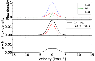
Figure 11: Approximation of the convolution function for the special case where a stellar line is blended by a telluric line ($\mu_{s}=\mu_{t}$). Upper panel: Artificial line profiles representing a stellar line (red line), a telluric line (dashed green line), and the instrumental line profile (dotted blue line, normalized for the sake of clarity). Middle panel: Left and right side of Eq. (14). Lower panel: Difference between the left and right side of Eq. (14) expressed by $a-b$. The dashed line indicates the limit set by the product of the line depths, $d_{s}d_{t}\sigma_{s}\sigma_{t}\sigma_{z}^{-2}$.

Assuming a perfectly blended stellar and telluric line $\mu_{s}=\mu_{t}=\lambda$, we obtain for the difference between Eq. (18) and Eq. (22)

$$a-b = \frac{A_{s}A_{t}}{2\pi\sigma_{z}^{2}}\left(1-\frac{1}{\sqrt{1+\frac{\sigma_{L}^{4}}{\sigma_{z}^{4}}}}\right)$$ (23)

$$= d_{s}d_{t}\frac{\sigma_{s}\sigma_{t}}{\sigma_{z}^{2}}\left(1-\frac{1}{\sqrt{1+\frac{\sigma_{L}^{4}}{\sigma_{z}^{4}}}}\right)\;,$$

where $d_{s,t}$ denote the line depths,

$$d_{s,t}=\frac{A_{s,t}}{\sqrt{2\pi\sigma_{s,t}^{2}}}\;.$$ (24)

In general, $\sigma_{z}^{2}\geq\sigma_{s}\sigma_{t}$, and we find $a-b\geq 0$, from which it follows that $a-b<d_{s}d_{t}\sigma_{s}\sigma_{t}\sigma_{z}^{-2}$. Under the stated assumptions, we therefore find that the accuracy of the approximation depends on the product of the line depths. This also follows from the linearity of the convolution operator in Eq. (14).

In Fig. 11, we illustrate the differences between the two sides of Eq. (14) for the special case of a central blend of a stellar and a telluric line (i.e., $\mu_{s}=\mu_{t}$) for parameters appropriate for the CARMENES spectrograph. In our approximation, we consider only normal line profiles. We choose the standard deviation of the instrumental line profile, $\sigma_{L}$, such that its FWHM matches that of the true VIS channel Voigt line profile of CARMENES (Table 2), which yields $\sigma_{L}=0.048\,$Å. We assumed stellar and telluric lines located at $\mu_{s}=\mu_{t}=10\,000\,$Å with line depths of $d_{s}=0.3$ and $d_{t}=0.3$. The intrinsic stellar and telluric line widths (before convolution by the instrumental LSF) were estimated from a synthetic PHOENIX spectrum (Husser et al. 2013) and a telluric transmission model, which yields $\sigma_{s}=0.05\,$Å and $\sigma_{t}=0.01\,$Å. We present the resulting Gaussian profiles in the upper panel of Fig. 11, the left and right side of Eq. (14) in the middle panel of Fig. 11, and the difference $a-b$ as well as the limit expressed by $d_{s}d_{t}\sigma_{s}\sigma_{t}\sigma_{z}^{-2}$ in the lower panel of Fig. 11. For the adopted parameters, the difference between the left and right side of Eq. (14) is approximately 0.5 %. This is in the range of $2$ % cited as the correction accuracy of molecfit. For shallower lines, the effect is less pronounced. In the extreme case of a very high instrument resolution represented by the limit $\sigma_{L}\rightarrow 0$, we find that $\sigma_{z}^{2}$ approaches $\sigma_{g}\sigma_{h}$ so that Eq. (23) approaches zero and the difference vanishes.

Our results allow obtaining an estimate of the accuracy of the approximation in Eq. (14) based on a normal approximation of the line profiles. They are also consistent with the findings of Sameshima et al. (2018).

Appendix B Additional figures

Appendix C Table of sample stars

Table 3: CARMENES M-dwarf sample of high S/N template spectra corrected for telluric absorption.

$\#$	Karmn	Name	GJ	$\alpha$	$\delta$	Spectral type	$J$ [mag]	$\#$ VIS obs	S$/$N	$\#$ NIR obs	S$/$N
1	J00051+457	BD+44 4548	2	00 05 10.89	+45 47 11.6	M1.0	6.70	53	833	44	756
2	J00067-075	GJ 1002	1002	00 06 43.20	-07 32 17.0	M5.5	8.32	91	641	80	948
3	J00162+198E	LP 404-062	1006B	00 16 16.15	+19 51 50.5	M4.0	8.89	19	295	17	333
4	J00183+440	GX And	15A	00 18 22.88	+44 01 22.6	M1.0	4.85	222	2040	196	2230
5	J00184+440	GQ And	15B	00 18 25.82	+44 01 38.1	M3.5	6.79	195	1539	179	1972
6	J00286-066	GJ 1012	1012	00 28 39.46	-06 39 49.2	M4.0	8.04	50	714	43	803
7	J00389+306	Wolf 1056	26	00 38 59.04	+30 36 58.4	M2.5	7.45	61	911	55	944
8	J00403+612	2MASS J00402129+6112490		00 40 21.29	+61 12 49.1	M1.5	10.15	46	233	42	182
9	J00570+450	G 172-030		00 57 02.69	+45 05 09.8	M3.0	8.10	20	432	17	495
10	J01013+613	GJ 47	47	01 01 20.05	+61 21 56.7	M2.0	7.27	10	307	9	251
11	J01019+541	G 218-020	3069	01 01 59.49	+54 10 57.7	M5.0	9.78	21	202	18	279
12	J01025+716	Ross 318	48	01 02 32.24	+71 40 47.3	M3.0	6.30	120	1183	103	1231
13	J01026+623	BD+61 195	49	01 02 38.87	+62 20 42.2	M1.5	6.23	83	927	80	969
14	J01033+623	V388 Cas	51	01 03 19.84	+62 21 55.8	M5.0	8.61	26	302	23	368
15	J01048-181	GJ 1028	1028	01 04 53.80	-18 07 28.6	M5.0	9.39	112	389	98	438
16	J01066+192	LSPM J0106+1913		01 06 36.98	+19 13 33.2	M3.0	9.34	66	428	59	403
17	J01078+128	G 2-21		01 07 52.23	+12 52 51.8	M1.5	8.79	17	328	14	254
18	J01125-169	YZ Cet	54.1	01 12 30.64	-16 59 56.4	M4.5	7.26	113	974	101	1197
19	J01339-176	LP 768-113		01 33 58.00	-17 38 23.8	M4.0	8.84	29	342	27	440
20	J01352-072	Barta 161 12		01 35 13.92	-07 12 51.5	M4.0	8.96	11	218	10	290
21	J01433+043	GJ 70	70	01 43 20.18	+04 19 18.0	M2.0	7.37	35	695	30	725
22	J01518+644	G 244-037	3117	01 51 51.13	+64 26 05.9	M2.5	7.84	60	780	55	765
23	J01550+379	LSR J0155+3758		01 55 02.33	+37 58 02.3	M5.0	10.47	9	70	9	77
24	J02002+130	TZ Ari	83.1	02 00 12.96	+13 03 07.0	M3.5	7.51	92	975	85	1309
25	J02015+637	G 244-047	3126	02 01 35.34	+63 46 12.0	M3.0	7.26	50	763	45	832
26	J02022+103	LP 469-067	3128	02 02 16.24	+10 20 13.9	M5.5	9.84	12	91	12	104
27	J02070+496	G 173-037		02 07 03.86	+49 38 43.5	M3.5	8.37	31	460	26	517
28	J02088+494	G 173-039	3136	02 08 53.62	+49 26 56.4	M3.5	8.42	17	341	14	407
29	J02123+035	BD+02 348	87	02 12 20.99	+03 34 32.2	M1.5	6.83	66	929	53	889
30	J02164+135	LP 469-206	3146	02 16 29.85	+13 35 12.8	M5.5	9.87	8	57	8	87
31	J02222+478	BD+47 612	96	02 22 14.64	+47 52 48.1	M0.5	6.38	55	696	41	669
32	J02336+249	GJ 102	102	02 33 37.18	+24 55 37.7	M4.0	8.47	30	442	28	520
33	J02358+202	BD+19 381	104	02 35 53.31	+20 13 11.6	M2.0	7.21	39	724	32	689
34	J02362+068	BX Cet	105	02 36 15.27	+06 52 17.9	M4.0	7.33	50	723	42	825
35	J02442+255	VX Ari	109	02 44 15.51	+25 31 24.1	M3.0	6.75	52	722	50	882
36	J02465+164	LP 411-006	3181	02 46 34.71	+16 25 10.2	M6.0	10.97	18	54	18	74
37	J02486+621	2MASS J02483695+6211228		02 48 36.99	+62 11 22.9	M5.0	12.51	6	9	6	9
38	J02489-145E	PM J02489-1432E		02 48 59.83	-14 32 16.2	M2.5	9.73	24	188	22	192
39	J02489-145W	PM J02489-1432W		02 48 59.27	-14 32 14.9	M2.0	9.53	34	241	30	218
40	J02519+224	RBS 365		02 51 54.10	+22 27 29.9	M4.0	8.92	15	272	15	352
41	J02530+168	Teegarden’s Star		02 53 00.89	+16 52 52.6	M7.0	8.39	272	973	251	1569
42	J02560-006	LP 591-156		02 56 03.90	-00 36 33.1	M5.0	10.42	6	49	6	50
43	J02565+554W	Ross 364	119A	02 56 34.42	+55 26 14.1	M1.0	7.42	10	271	6	112
44	J02573+765	G 245-61		02 57 18.26	+76 33 11.3	M3.0	9.62	58	304	56	323
45	J03090+100	GJ 1055	1055	03 09 00.17	+10 01 25.7	M5.0	9.93	8	93	6	80

Table 4: Continued.

$\#$	Karmn	Name	GJ	$\alpha$	$\delta$	Spectral type	$J$ [mag]	$\#$ VIS obs	S$/$N	$\#$ NIR obs	S$/$N
46	J03133+047	CD Cet	1057	03 13 22.92	+04 46 29.3	M5.0	8.78	110	651	105	920
47	J03142+286	LP 299-036	3208	03 14 12.47	+28 40 39.6	M6.0	10.99	10	38	9	43
48	J03181+382	HD 275122	134	03 18 07.48	+38 15 07.4	M1.5	7.02	56	905	50	942
49	J03213+799	GJ 133	133	03 21 21.78	+79 58 02.2	M2.0	7.70	33	563	31	632
50	J03217-066	G 77-046	3218	03 21 46.92	-06 40 24.2	M2.0	7.86	15	399	13	426
51	J03230+420	GJ 1059	1059	03 23 01.76	+42 00 26.8	M5.0	10.39	12	77	12	79
52	J03463+262	HD 23453	154	03 46 20.14	+26 12 55.8	M0.0	6.69	49	781	46	930
53	J03473+086	LTT 11262	3250	03 47 20.89	+08 41 47.1	M4.5	9.85	9	96	8	74
54	J03473-019	G 80-021		03 47 23.34	-01 58 19.9	M3.0	7.80	11	278	9	346
55	J03531+625	Ross 567		03 53 10.44	+62 34 08.1	M3.0	7.78	39	662	37	776
56	J04153-076	omi02 Eri C	166C	04 15 21.54	-07 39 20.7	M4.5	6.75	53	550	54	759
57	J04167-120	LP 714-47		04 16 45.60	-12 05 02.5	M0.0	9.49	35	271	33	227
58	J04198+425	LSR J0419+4233		04 19 52.13	+42 33 30.4	M8.5	11.09	35	51	42	112
59	J04225+105	LSPM J0422+1031		04 22 31.99	+10 31 18.8	M3.5	8.47	18	327	14	396
60	J04290+219	BD+21 652	169	04 29 00.12	+21 55 21.7	M0.5	5.67	170	1491	151	1398
61	J04311+589	G 175-34	169.1A	04 31 11.51	+58 58 37.5	M4.0	6.62	11	312	9	214
62	J04343+430	PM J04343+4302		04 34 22.50	+43 02 14.7	M2.5	9.62	56	317	55	283
63	J04376+528	BD+52 857	172	04 37 40.93	+52 53 37.0	M0.0	5.87	126	1273	97	1332
64	J04376-110	BD-11 916	173	04 37 41.87	-11 02 20.0	M1.5	6.94	43	726	39	681
65	J04406-128	TOI-2457		04 40 40.14	-12 53 26.9	M0.0	9.74	53	266	53	228
66	J04429+189	HD 285968	176	04 42 55.77	+18 57 29.4	M2.0	6.46	23	451	16	424
67	J04429+214	2MASS J04425586+2128230		04 42 55.86	+21 28 23.0	M3.5	7.96	16	327	15	353
68	J04472+206	RX J0447.2+2038		04 47 12.25	+20 38 10.8	M5.0	9.38	11	153	11	226
69	J04520+064	Wolf 1539	179	04 52 05.73	+06 28 35.6	M3.5	7.81	10	269	10	313
70	J04538-177	GJ 180	180	04 53 49.98	-17 46 24.3	M2.0	7.41	25	578	22	663
71	J04588+498	BD+49 1280	181	04 58 50.57	+49 50 57.4	M0.0	6.92	56	900	49	1011
72	J05019+011	1RXS J050156.7+010845		05 01 56.66	+01 08 42.9	M4.0	8.53	19	305	19	425
73	J05019-069	LP 656-038	3323	05 01 57.43	-06 56 46.4	M4.0	7.62	8	261	7	276
74	J05033-173	LP 776-046	3325	05 03 20.08	-17 22 24.7	M3.0	7.82	68	795	81	799
75	J05062+046	RX J0506.2+0439		05 06 12.93	+04 39 27.2	M4.0	8.91	13	201	11	289
76	J05084-210	2MASS J05082729-2101444		05 08 27.30	-21 01 44.4	M5.0	9.72	39	161	36	244
77	J05127+196	GJ 192	192	05 12 42.23	+19 39 56.4	M2.0	7.30	43	715	36	695
78	J05280+096	Ross 41	203	05 28 00.15	+09 38 38.2	M3.5	8.31	17	335	14	416
79	J05314-036	HD 36395	205	05 31 27.40	-03 40 38.0	M1.5	4.72	95	1175	77	1175
80	J05348+138	Ross 46	3356	05 34 52.12	+13 52 46.7	M3.5	7.78	21	507	17	577
81	J05360-076	Wolf 1457	3357	05 36 00.08	-07 38 58.4	M4.0	8.46	39	451	32	523
82	J05365+113	V2689 Ori	208	05 36 30.99	+11 19 40.3	M0.0	6.13	131	1398	113	1507
83	J05366+112	PM J05366+1117		05 36 38.46	+11 17 48.8	M4.0	8.27	16	370	13	460
84	J05394+406	LSR J0539+4038		05 39 24.80	+40 38 42.8	M8.0	11.11	21	53	29	114
85	J05415+534	HD 233153	212	05 41 30.73	+53 29 23.3	M1.0	6.59	97	1176	81	1203
86	J05421+124	V1352 Ori	213	05 42 09.27	+12 29 21.6	M4.0	7.12	51	731	46	893
87	J06000+027	G 99-049	3379	06 00 03.50	+02 42 23.6	M4.0	6.91	14	303	13	411
88	J06011+595	G 192-013	3378	06 01 11.05	+59 35 49.9	M3.5	7.46	80	900	74	1107
89	J06024+498	G 192-015	3380	06 02 29.19	+49 51 56.2	M5.0	9.35	125	459	117	503
90	J06103+821	GJ 226	226	06 10 19.85	+82 06 24.3	M2.0	6.87	57	809	55	999

Table 5: Continued.

$\#$	Karmn	Name	GJ	$\alpha$	$\delta$	Spectral type	$J$ [mag]	$\#$ VIS obs	S$/$N	$\#$ NIR obs	S$/$N
91	J06105-218	HD 42581	229A	06 10 34.61	-21 51 52.7	M0.5	5.10	51	742	45	821
92	J06246+234	Ross 64	232	06 24 41.28	+23 25 58.9	M4.0	8.66	9	215	9	263
93	J06318+414	LP 205-044	3396	06 31 50.74	+41 29 45.5	M5.0	9.68	37	237	36	362
94	J06371+175	HD 260655	239	06 37 10.80	+17 33 53.3	M0.0	6.67	125	1253	112	1331
95	J06396-210	LP 780-032		06 39 37.43	-21 01 34.1	M4.0	8.51	58	446	55	576
96	J06421+035	G 108-021	3404A	06 42 11.19	+03 34 52.6	M3.5	8.17	19	453	13	487
97	J06548+332	Wolf 294	251	06 54 48.96	+33 16 05.4	M3.0	6.10	444	2310	398	2383
98	J06574+740	2MASS J06572616+7405265		06 57 26.12	+74 05 26.6	M4.0	8.93	13	228	12	300
99	J06594+193	GJ 1093	1093	06 59 28.82	+19 20 55.9	M5.0	9.16	30	285	26	419
100	J07033+346	LP 255-011	3423	07 03 23.17	+34 41 51.4	M4.0	8.77	14	302	14	375
101	J07044+682	GJ 258	258	07 04 25.94	+68 17 19.7	M3.0	8.17	18	378	13	415
102	J07051-101	2MASS J07051194-1007528		07 05 11.96	-10 07 52.8	M5.0	10.20	11	62	10	80
103	J07274+052	Luyten’s Star	273	07 27 24.50	+05 13 32.8	M3.5	5.71	774	1217	756	1725
104	J07287-032	GJ 1097	1097	07 28 45.44	-03 17 53.3	M3.0	7.54	25	517	24	651
105	J07319+362N	V* BL Lyn	277B	07 31 57.32	+36 13 47.4	M3.5	7.57	50	749	48	911
106	J07353+548	GJ 3452	3452	07 35 21.88	+54 50 59.0	M2.0	7.77	10	320	10	312
107	J07386-212	LP 763-001	3459	07 38 40.96	-21 13 28.5	M3.0	7.85	7	224	7	298
108	J07393+021	BD+02 1729	281	07 39 23.04	+02 11 01.2	M0.0	6.77	51	823	43	829
109	J07403-174	LP 783-002	283B	07 40 19.37	-17 24 45.9	M6.0	10.15	53	125	54	218
110	J07446+035	YZ CMi	285	07 44 40.17	+03 33 08.9	M4.5	6.58	51	638	39	803
111	J07472+503	2MASS J07471385+5020386		07 47 13.87	+50 20 38.5	M4.0	8.86	15	293	16	410
112	J07558+833	GJ 1101	1101	07 55 53.93	+83 23 04.9	M4.5	8.74	14	234	14	331
113	J07582+413	GJ 1105	1105	07 58 12.70	+41 18 13.3	M3.5	7.73	28	479	27	610
114	J07590+153	LP 424-004	3470	07 59 05.84	+15 23 29.2	M1.5	8.79	107	449	65	420
115	J08023+033	G 50-16 A	3473	08 02 22.88	+03 20 19.7	M4.0	9.63	67	307	61	293
116	J08119+087	Ross 619	299	08 11 57.57	+08 46 23.0	M4.5	8.42	16	341	15	432
117	J08126-215	GJ 300	300	08 12 40.89	-21 33 07.0	M4.0	7.60	18	366	16	472
118	J08161+013	GJ 2066	2066	08 16 07.98	+01 18 09.3	M2.0	6.62	75	974	70	1136
119	J08293+039	2MASS J08292191+0355092		08 29 21.91	+03 55 09.3	M2.5	7.93	15	445	12	497
120	J08298+267	DX Cnc	1111	08 29 49.35	+26 46 33.6	M6.5	8.23	35	382	29	632
121	J08315+730	LP 035-219		08 31 30.12	+73 03 45.8	M4.0	8.78	19	305	18	375
122	J08358+680	G 234-037	3506	08 35 49.04	+68 04 09.1	M2.5	7.86	11	303	11	361
123	J08402+314	LSPM J0840+3127		08 40 15.98	+31 27 06.8	M3.5	8.12	8	281	6	336
124	J08409-234	LP 844-008	317	08 40 59.21	-23 27 22.6	M3.5	7.93	36	439	35	488
125	J08413+594	LP 090-018	3512	08 41 20.13	+59 29 50.4	M5.5	9.62	222	460	207	703
126	J08526+283	rho Cnc B	324B	08 52 40.86	+28 18 58.8	M4.5	8.56	11	264	10	324
127	J08536-034	LP 666-009	3517	08 53 36.16	-03 29 32.2	M9.0	11.21	45	32	43	82
128	J08599+729	LP 036-098	3520	08 59 56.20	+72 57 36.3	M4.0	9.73	18	140	17	116
129	J09003+218	LP 368-128		09 00 23.55	+21 50 04.9	M6.5	9.44	25	156	20	263
130	J09005+465	GJ 1119	1119	09 00 32.48	+46 35 11.1	M4.5	8.60	8	201	8	269
131	J09028+680	LP 060-179	3526	09 02 52.87	+68 03 46.6	M4.0	8.45	10	276	11	393
132	J09033+056	NLTT 20861		09 03 20.96	+05 40 14.6	M7.0	10.77	31	80	27	119
133	J09133+688	G 234-57A		09 13 23.86	+68 52 31.0	M2.5	7.78	16	397	16	472
134	J09143+526	HD 79210	338A	09 14 22.77	+52 41 11.8	M0.0	4.89	72	747	65	868
135	J09144+526	HD 79211	338B	09 14 24.68	+52 41 10.9	M0.0	4.78	158	1363	128	1384

Table 6: Continued.

$\#$	Karmn	Name	GJ	$\alpha$	$\delta$	Spectral type	$J$ [mag]	$\#$ VIS obs	S$/$N	$\#$ NIR obs	S$/$N
136	J09161+018	RX J0916.1+0153		09 16 10.18	+01 53 08.8	M4.0	8.77	9	199	9	277
137	J09163-186	LP 787-052	3543	09 16 20.64	-18 37 32.9	M1.5	7.35	5	249	4	115
138	J09286-121	G 161-32		09 28 41.58	-12 09 55.1	M2.5	8.84	7	156	7	124
139	J09307+003	GJ 1125	1125	09 30 44.59	+00 19 21.6	M3.5	7.70	22	472	22	584
140	J09360-216	GJ 357	357	09 36 01.64	-21 39 38.9	M2.5	7.34	26	621	25	520
141	J09411+132	Ross 85	361	09 41 10.36	+13 12 34.4	M1.5	6.97	49	824	44	807
142	J09423+559	GJ 363	363	09 42 23.19	+55 59 01.3	M3.5	8.37	10	275	10	377
143	J09425+700	GJ 360	360	09 42 34.84	+70 02 02.0	M2.0	6.92	49	703	42	737
144	J09428+700	GJ 362	362	09 42 51.73	+70 02 21.9	M3.0	7.33	51	754	50	787
145	J09439+269	Ross 93	3564	09 43 55.61	+26 58 08.4	M3.5	8.04	6	229	7	316
146	J09447-182	GJ 1129	1129	09 44 47.35	-18 12 49.0	M4.0	8.12	12	303	11	395
147	J09449-123	G 161-071		09 44 54.19	-12 20 54.4	M5.0	8.50	10	181	10	290
148	J09468+760	BD+76 3952	366	09 46 48.49	+76 02 38.1	M1.5	7.44	26	580	23	550
149	J09511-123	BD-11 2741	369	09 51 09.64	-12 19 47.5	M0.5	6.99	25	598	20	485
150	J09535+355	Wolf 327		09 53 30.91	+35 34 16.7	M2.5	9.31	24	246	19	216
151	J09561+627	BD+63 869	373	09 56 08.67	+62 47 18.5	M0.0	6.03	69	898	65	898
152	J09597+472	G 146-005	3579	09 59 45.99	+47 12 11.3	M4.0	9.76	11	115	11	97
153	J10023+480	BD+48 1829	378	10 02 21.75	+48 05 19.7	M1.0	6.95	22	515	17	541
154	J10087+355	Wolf 346		15 .1 6308	35. 47 62	M1.5	9.17	13	180	13	157
155	J10088+692	TYC 4384-1735-1		10 08 51.81	+69 16 35.6	M0.5	8.71	41	498	36	491
156	J10122-037	AN Sex	382	10 12 17.67	-03 44 44.4	M1.5	5.89	76	944	60	954
157	J10125+570	LP 092-048		10 12 34.78	+57 03 49.0	M3.5	7.76	10	305	9	337
158	J10167-119	GJ 386	386	10 16 45.95	-11 57 42.4	M3.0	7.32	20	510	19	448
159	J10185-117	LP 729-54		10 18 35.14	-11 43 00.2	M4.0	9.01	51	407	51	450
160	J10196+198	AD Leo	388	10 19 36.28	+19 52 12.0	M3.0	5.45	85	615	79	654
161	J10238+438	LP 212-062		10 23 51.86	+43 53 33.1	M5.0	10.04	11	78	9	66
162	J10251-102	BD-09 3070	390	10 25 10.84	-10 13 43.3	M1.0	6.89	29	652	28	620
163	J10289+008	BD+01 2447	393	10 28 55.55	+00 50 27.6	M2.0	6.18	85	990	78	1060
164	J10350-094	LP 670-017		10 35 01.12	-09 24 38.6	M3.0	8.28	16	361	13	459
165	J10360+051	RY Sex	398	10 36 01.22	+05 07 12.8	M3.5	8.46	7	201	7	297
166	J10396-069	GJ 399	399	10 39 40.56	-06 55 25.5	M2.5	7.66	7	277	7	337
167	J10416+376	GJ 1134	1134	10 41 37.88	+37 36 39.2	M4.5	8.49	11	255	9	287
168	J10482-113	LP 731-058	3622	10 48 12.61	-11 20 09.6	M6.5	8.86	79	334	72	630
169	J10508+068	EE Leo	402	10 50 52.03	+06 48 29.3	M4.0	7.32	53	806	49	1007
170	J10564+070	CN Leo	406	10 56 28.92	+07 00 53.0	M6.0	7.08	78	644	63	1034
171	J10584-107	LP 731-076		10 58 27.99	-10 46 30.5	M5.0	9.51	53	252	49	344
172	J11000+228	Ross 104	408	11 00 04.26	+22 49 58.6	M2.5	6.31	60	793	50	869
173	J11026+219	DS Leo	410	11 02 38.34	+21 58 01.7	M1.0	6.52	53	791	43	858
174	J11033+359	Lalande 21185	411	11 03 20.19	+35 58 11.5	M1.5	4.10	565	2731	505	2940
175	J11044+304	LSPM J1104+3027		11 04 28.55	+30 27 31.5	M3.0	10.93	94	149	91	157
176	J11054+435	BD+44 2051A	412A	11 05 28.58	+43 31 36.4	M1.0	5.54	118	1130	106	1246
177	J11055+435	WX UMa	412B	11 05 30.89	+43 31 17.9	M5.5	8.74	60	356	55	513
178	J11108+479	G 176-015	3646	11 10 51.52	+47 57 02.0	M4.0	10.08	11	99	8	79
179	J11110+304E	HD 97101A	414A	11 11 05.17	+30 26 45.7	K7.0	5.76	13	465	12	563
180	J11110+304W	HD 97101B	414B	11 11 02.54	+30 26 41.3	M2.0	6.59	51	760	48	832

Table 7: Continued.

$\#$	Karmn	Name	GJ	$\alpha$	$\delta$	Spectral type	$J$ [mag]	$\#$ VIS obs	S$/$N	$\#$ NIR obs	S$/$N
181	J11126+189	StKM 1-928	3649	11 12 38.97	+18 56 05.4	M1.5	7.45	20	542	16	616
182	J11195+466	LP 169-022		11 19 30.61	+46 41 43.1	M5.5	10.09	5	44	4	42
183	J11201-104	LP 733-099		11 20 06.10	-10 29 46.7	M2.0	7.81	27	496	25	545
184	J11289+101	Wolf 398	3666	11 28 56.26	+10 10 39.2	M3.5	8.48	9	252	8	282
185	J11302+076	K2-18		11 30 14.52	+07 35 18.3	M2.5	9.76	63	305	61	394
186	J11306-080	LP 672-042		11 30 41.83	-08 05 43.0	M3.5	8.03	15	358	13	421
187	J11417+427	Ross 1003	1148	11 41 44.64	+42 45 07.1	M4.0	7.61	80	925	70	1206
188	J11421+267	Ross 905	436	11 42 11.09	+26 42 23.7	M2.5	6.90	444	1404	400	1827
189	J11423+230	LP 375-23		11 42 18.37	+23 01 36.7	M0.5	8.65	86	671	77	606
190	J11467-140	GJ 443	443	11 46 42.91	-14 00 51.8	M3.0	7.96	15	386	15	492
191	J11474+667	1RXS J114728.8+664405		11 47 28.57	+66 44 02.7	M5.0	9.68	54	221	49	292
192	J11476+002	LP 613-49A	3685A	11 47 40.75	+00 15 20.1	M4.0	8.99	7	150	7	186
193	J11476+786	GJ 445	445	11 47 41.39	+78 41 28.2	M3.5	6.72	66	774	53	942
194	J11477+008	FI Vir	447	11 47 44.40	+00 48 16.4	M4.0	6.50	56	704	50	880
195	J11509+483	GJ 1151	1151	11 50 57.72	+48 22 38.6	M4.5	8.49	117	670	106	757
196	J11511+352	BD+36 2219	450	11 51 07.34	+35 16 19.2	M1.5	6.42	112	1123	101	1345
197	J12054+695	Ross 689	3704	12 05 29.68	+69 32 22.6	M4.0	8.74	7	180	6	217
198	J12100-150	LP 734-032	3707	12 10 05.60	-15 04 17.0	M3.5	7.77	67	670	61	724
199	J12111-199	LTT 4562	3708A	12 11 11.76	-19 57 38.1	M3.0	7.89	19	395	18	444
200	J12123+544S	HD 238090	458A	12 12 20.86	+54 29 08.7	M0.0	6.88	111	1221	100	1408
201	J12156+526	StKM 2-809		12 15 39.36	+52 39 08.8	M4.0	8.59	13	247	12	310
202	J12189+111	GL Vir	1156	12 18 59.40	+11 07 33.8	M5.0	8.53	13	233	10	344
203	J12230+640	Ross 690	463	12 23 00.16	+64 01 51.0	M3.0	7.94	160	884	147	1505
204	J12248-182	Ross 695	465	12 24 52.50	-18 14 32.3	M2.0	7.73	15	370	14	436
205	J12312+086	BD+09 2636	471	12 31 15.81	+08 48 38.2	M0.5	6.78	48	804	41	899
206	J12350+098	GJ 476	476	12 35 00.71	+09 49 42.6	M2.5	8.00	10	307	8	321
207	J12373-208	LP 795-038		12 37 21.57	-20 52 35.5	M4.0	8.97	19	193	16	213
208	J12388+116	Wolf 433	480	12 38 52.44	+11 41 46.1	M3.0	7.58	11	383	11	364
209	J12428+418	G 123-055		12 42 49.88	+41 53 47.1	M4.0	8.12	9	254	8	291
210	J12479+097	Wolf 437	486	12 47 56.62	+09 45 05.0	M3.5	7.20	105	1045	97	1257
211	J13005+056	FN Vir	493.1	13 00 33.52	+05 41 08.0	M4.5	8.55	12	183	9	200
212	J13102+477	G 177-025		13 10 12.63	+47 45 18.7	M5.0	9.58	36	243	34	327
213	J13119+658	PM J13119+6550		13 11 59.56	+65 50 01.7	M3.0	9.71	12	140	11	147
214	J13196+333	Ross 1007	507.1	13 19 40.13	+33 20 47.5	M1.5	7.27	9	278	6	299
215	J13209+342	BD+35 2439	508.2	13 20 58.05	+34 16 44.2	M1.0	7.40	16	469	15	415
216	J13229+244	Ross 1020	3779	13 22 56.75	+24 28 03.6	M4.0	8.73	112	712	105	959
217	J13255+688	2MASS J13253177+6850106		13 25 31.78	+68 50 10.6	M0.0	10.04	70	265	65	239
218	J13283-023W	Ross 486A	512A	13 28 21.08	-02 21 37.1	M3.0	7.51	12	344	10	322
219	J13293+114	GJ 513	513	13 29 21.31	+11 26 26.7	M3.5	8.37	6	201	6	215
220	J13299+102	BD+11 2576	514	13 29 59.79	+10 22 37.8	M0.5	5.90	447	2431	417	2425
221	J13300-087	Ross 476	514.1	13 30 02.80	-08 42 25.5	M4.0	9.60	8	104	6	62
222	J13427+332	Ross 1015	3801	13 42 43.27	+33 17 24.3	M3.5	7.79	19	433	15	509
223	J13450+176	BD+18 2776	525	13 45 05.08	+17 47 07.6	M0.0	7.00	31	686	28	707
224	J13457+148	HD 119850	526	13 45 43.78	+14 53 29.5	M1.5	5.18	250	1796	199	1785
225	J13458-179	LP 798-034	3804	13 45 50.71	-17 58 05.6	M3.5	7.75	11	268	10	334

Table 8: Continued.

$\#$	Karmn	Name	GJ	$\alpha$	$\delta$	Spectral type	$J$ [mag]	$\#$ VIS obs	S$/$N	$\#$ NIR obs	S$/$N
226	J13536+776	RX J1353.6+7737		13 53 38.79	+77 37 08.2	M4.0	8.63	25	331	24	440
227	J13582+125	Ross 837	3817	13 58 13.92	+12 34 43.9	M3.0	8.27	10	282	8	265
228	J13591-198	LP 799-007	3820	13 59 10.41	-19 50 03.7	M4.0	8.33	17	230	17	317
229	J14010-026	HD 122303	536	14 01 03.19	-02 39 17.5	M1.0	6.52	27	490	25	602
230	J14082+805	BD+81 465	540	14 08 12.98	+80 35 50.2	M1.0	7.18	37	661	32	638
231	J14152+450	Ross 992	3836	14 15 16.98	+45 00 53.3	M3.0	8.01	9	297	8	327
232	J14173+454	RX J1417.3+4525		14 17 22.10	+45 25 46.0	M5.0	9.47	12	154	9	209
233	J14251+518	tet Boo B	549B	14 25 11.58	+51 49 53.1	M2.5	7.88	13	390	12	475
234	J14257+236E	BD+24 2733B	548B	14 25 46.65	+23 37 13.7	M0.5	6.89	49	810	41	774
235	J14257+236W	BD+24 2733A	548A	14 25 43.47	+23 37 01.5	M0.0	6.77	64	902	57	993
236	J14294+155	Ross 130	552	14 29 29.70	+15 31 57.5	M2.0	7.23	6	234	5	258
237	J14307-086	BD-07 3856	553	14 30 47.72	-08 38 46.8	M0.5	6.62	93	1101	85	1230
238	J14310-122	Wolf 1478	553.1	14 31 01.16	-12 17 46.0	M3.5	7.80	6	218	5	232
239	J14321+081	LP 560-035		14 32 08.51	+08 11 31.2	M6.0	10.11	58	169	58	259
240	J14342-125	HN Lib	555	14 34 16.81	-12 31 10.4	M4.0	6.84	98	974	84	1258
241	J14524+123	G 66-37	3871	14 52 28.53	+12 23 32.8	M2.0	7.97	26	491	20	480
242	J14544+355	Ross 1041	3873	14 54 27.91	+35 32 57.0	M3.5	8.24	33	544	32	688
243	J14578+566	GJ 1187	1187	14 57 53.73	+56 39 24.5	M5.5	10.21	7	67	7	64
244	J15013+055	G 15-2	3885	15 01 20.11	+05 32 55.5	M3.0	8.33	19	393	17	419
245	J15095+031	Ross 1047	3892	15 09 35.59	+03 10 00.6	M3.0	7.72	17	409	16	408
246	J15100+193	G 136-072	3893	15 10 04.82	+19 21 27.5	M4.0	9.06	10	183	10	146
247	J15194-077	HO Lib	581	15 19 26.83	-07 43 20.2	M3.0	6.71	52	794	45	954
248	J15218+209	OT Ser	9520	15 21 52.93	+20 58 39.9	M1.5	6.61	53	766	48	757
249	J15238+174	Ross 508	585	15 23 51.14	+17 27 57.4	M4.5	9.11	6	142	6	126
250	J15305+094	NLTT 40406		15 30 30.33	+09 26 01.4	M5.5	9.57	14	140	12	215
251	J15369-141	Ross 802	592	15 36 58.62	-14 08 01.8	M4.0	8.43	9	193	5	188
252	J15499+796	LP 022-420		15 49 55.14	+79 39 51.6	M5.0	9.72	15	126	14	206
253	J15583+354	G 180-018	3929	15 58 18.80	+35 24 24.3	M3.5	8.69	82	568	74	585
254	J15598-082	BD-07 4156	606	15 59 53.38	-08 15 11.5	M1.0	7.18	24	582	19	477
255	J16028+205	GJ 609	609	16 02 50.94	+20 35 21.0	M4.0	8.13	26	458	24	527
256	J16092+093	G 137-084		16 09 16.27	+09 21 07.5	M3.0	7.97	9	281	6	176
257	J16102-193	K2-33		16 10 14.74	-19 19 09.4	M3.0	11.10	27	41	26	59
258	J16167+672N	EW Dra	617B	16 16 45.31	+67 15 22.5	M3.0	6.91	107	1060	103	1121
259	J16167+672S	HD 147379	617A	16 16 42.75	+67 14 19.8	M0.0	5.78	188	1667	179	1704
260	J16254+543	GJ 625	625	16 25 24.62	+54 18 14.8	M1.5	6.61	32	577	28	737
261	J16303-126	V2306 Oph	628	16 30 18.06	-12 39 45.3	M3.5	5.95	92	994	91	1204
262	J16313+408	G 180-060	3959	16 31 18.79	+40 51 51.7	M5.0	9.46	13	144	11	200
263	J16327+126	GJ 1203	1203	16 32 45.19	+12 36 46.0	M3.0	8.43	13	285	12	312
264	J16343+571	CM Dra	630.1A	16 34 20.33	+57 09 44.4	M4.5	8.50	45	201	43	277
265	J16462+164	LP 446-006	3972	16 46 13.74	+16 28 40.8	M2.5	7.95	17	443	16	442
266	J16554-083N	Wolf 629	643	16 55 25.22	-08 19 21.3	M3.5	7.55	31	540	27	675
267	J16555-083	VB 8	644C	16 55 35.26	-08 23 40.8	M7.0	9.78	128	241	110	398
268	J16570-043	LP 686-027	1207	16 57 05.74	-04 20 56.3	M3.5	7.97	15	344	12	443
269	J16578+473	HD 153557B	649.1B	16 57 53.61	+47 22 02.4	M1.5	6.87	9	440	8	467
270	J16581+257	BD+25 3173	649	16 58 08.85	+25 44 39.0	M1.0	6.45	55	883	49	1017

Table 9: Continued.

$\#$	Karmn	Name	GJ	$\alpha$	$\delta$	Spectral type	$J$ [mag]	$\#$ VIS obs	S$/$N	$\#$ NIR obs	S$/$N
271	J17033+514	G 203-042	3988	17 03 23.88	+51 24 22.9	M4.5	8.77	72	526	65	552
272	J17052-050	Wolf 636	654	17 05 13.78	-05 05 39.2	M1.5	6.78	50	776	46	838
273	J17071+215	Ross 863	655	17 07 07.49	+21 33 14.5	M3.0	7.88	15	413	15	422
274	J17115+384	Wolf 654	3992	17 11 34.75	+38 26 33.9	M3.5	7.63	77	942	66	949
275	J17166+080	GJ 2128	2128	17 16 40.98	+08 03 30.2	M2.0	7.93	19	457	17	469
276	J17198+417	GJ 671	671	17 19 52.71	+41 42 49.7	M2.5	7.71	20	467	17	489
277	J17303+055	BD+05 3409	678.1	17 30 22.73	+05 32 54.7	M0.0	6.24	55	821	57	987
278	J17338+169	1RXS J173353.5+165515		17 33 53.18	+16 55 13.1	M5.5	8.89	12	181	13	252
279	J17355+616	BD+61 1678	685	17 35 34.48	+61 40 53.6	M0.5	6.88	26	609	24	729
280	J17364+683	BD+68 946	687	17 36 25.90	+68 20 20.9	M3.0	5.33	41	631	36	645
281	J17378+185	BD+18 3421	686	17 37 53.35	+18 35 30.2	M1.0	6.36	106	1241	104	1471
282	J17481+159	2MASS J17481125+1558465		17 48 11.25	+15 58 46.7	M3.0	9.61	30	216	29	176
283	J17542+073	GJ 1222	1222	17 54 17.12	+07 22 44.8	M4.0	8.77	12	213	11	216
284	J17578+046	Barnard’s Star	699	17 57 48.50	+04 41 36.3	M3.5	5.24	766	2920	708	3270
285	J17578+465	G 204-039	4040	17 57 50.97	+46 35 19.1	M2.5	7.85	26	541	22	578
286	J18012+355	G 182-034		18 01 16.10	+35 35 50.5	M3.5	9.70	35	238	33	168
287	J18022+642	LP 071-082		18 02 16.60	+64 15 44.2	M5.0	8.54	28	344	26	487
288	J18027+375	GJ 1223	1223	18 02 46.26	+37 31 03.0	M5.0	9.72	122	395	114	406
289	J18051-030	HD 165222	701	18 05 07.58	-03 01 52.7	M1.0	6.16	56	839	57	1013
290	J18075-159	GJ 1224	1224	18 07 32.84	-15 57 47.1	M4.5	8.64	15	239	15	283
291	J18131+260	LP 390-16	4044	18 13 06.57	+26 01 51.9	M4.0	8.90	16	243	12	254
292	J18165+048	G 140-51		18 16 31.54	+04 52 45.8	M5.0	9.80	52	262	46	345
293	J18174+483	TYC 3529-1437-1		18 17 25.13	+48 22 02.3	M2.0	7.77	72	849	65	1061
294	J18180+387E	G 204-58	4048A	18 18 04.23	+38 46 32.6	M3.0	8.04	18	366	17	378
295	J18189+661	LP 71-165	4053	18 18 57.23	+66 11 33.3	M4.5	8.74	13	242	12	344
296	J18198-019	HD 168442	710	18 19 50.84	-01 56 19.0	K7.0	7.08	147	1596	141	1708
297	J18221+063	Ross 136	712	18 22 06.68	+06 20 37.6	M4.0	8.67	17	296	15	298
298	J18224+620	GJ 1227	1227	18 22 27.09	+62 03 01.7	M4.0	8.64	61	530	58	669
299	J18319+406	G 205-028	4062	18 31 58.38	+40 41 11.0	M3.5	8.06	20	438	17	460
300	J18346+401	LP 229-017	4063	18 34 36.65	+40 07 26.4	M3.5	7.18	79	960	73	1162
301	J18353+457	BD+45 2743	720A	18 35 18.39	+45 44 38.5	M0.5	6.88	16	484	16	579
302	J18356+329	LSR J1835+3259		18 35 37.88	+32 59 53.3	M8.5	10.27	59	87	63	202
303	J18363+136	Ross 149	4065	18 36 19.23	+13 36 26.4	M4.0	8.19	26	418	22	457
304	J18409-133	BD-13 5069	724	18 40 57.31	-13 22 46.6	M1.0	7.40	84	1006	81	814
305	J18419+318	Ross 145	4070	18 41 59.04	+31 49 49.8	M3.0	7.52	24	505	22	484
306	J18427+596N	HD 173739	725A	18 42 46.70	+59 37 49.4	M3.0	5.19	71	928	70	1006
307	J18427+596S	HD 173740	725B	18 42 46.89	+59 37 36.7	M3.5	5.72	77	966	72	933
308	J18480-145	G 155-042	4077	18 48 01.27	-14 34 51.2	M2.5	8.38	21	359	19	427
309	J18482+076	G 141-036		18 48 17.54	+07 41 21.2	M5.0	8.85	54	423	46	518
310	J18498-238	V1216 Sgr	729	18 49 49.36	-23 50 10.4	M3.5	6.22	56	788	51	817
311	J18580+059	BD+05 3993	740	18 58 00.14	+05 54 29.2	M0.5	6.24	34	608	30	673
312	J19025+754	LSPM J1902+7525		19 02 31.93	+75 25 07.0	M2.5	9.80	46	261	44	244
313	J19070+208	Ross 730	745A	19 07 05.56	+20 53 16.9	M2.0	7.29	38	703	33	681
314	J19072+208	HD 349726	745B	19 07 13.20	+20 52 37.3	M2.0	7.28	44	770	39	810
315	J19084+322	G 207-019	4098	19 08 29.93	+32 16 51.6	M3.0	7.91	24	484	23	529

Table 10: Continued.

$\#$	Karmn	Name	GJ	$\alpha$	$\delta$	Spectral type	$J$ [mag]	$\#$ VIS obs	S$/$N	$\#$ NIR obs	S$/$N
316	J19098+176	GJ 1232	1232	19 09 50.87	+17 40 06.4	M4.5	8.82	23	313	17	342
317	J19169+051N	V1428 Aql	752A	19 16 55.26	+05 10 08.0	M2.5	5.58	129	1304	114	1278
318	J19169+051S	V1298 Aql	752B	19 16 57.61	+05 09 01.6	M8.0	9.91	51	142	44	241
319	J19206+731S	2MASS J19204172+7311434		19 20 41.73	+73 11 43.5	M4.5	10.60	22	117	23	132
320	J19216+208	GJ 1235	1235	19 21 38.70	+20 52 03.3	M4.5	8.80	25	332	23	374
321	J19242+755	GJ 1238	1238	19 24 16.31	+75 33 11.8	M5.5	9.91	222	356	218	420
322	J19251+283	Ross 164	4109	19 25 08.48	+28 21 13.8	M3.0	8.44	26	439	25	492
323	J19255+096	LSPM J1925+0938		19 25 30.91	+09 38 23.3	M8.0	11.21	100	67	97	168
324	J19346+045	BD+04 4157	763	19 34 39.84	+04 34 57.0	M0.0	6.71	53	836	49	981
325	J19422-207	2MASS J19421282-2045477		19 42 12.82	-20 45 48.0	M5.1	9.60	27	170	24	182
326	J19511+464	G 208-042	1243	19 51 09.32	+46 29 00.2	M4.0	8.59	14	272	9	306
327	J19573-125	HD 188807 B	773B	19 57 23.80	-12 33 50.2	M5.0	10.21	8	36	8	50
328	J20093-012	2MASS J20091824-0113377		20 09 18.25	-01 13 38.3	M5.0	9.40	13	172	13	238
329	J20109+708	TYC 4450-1440-1		20 10 57.12	+70 52 09.8	K5.0	9.71	78	400	68	348
330	J20227+473	Ross 176		20 22 45.19	+47 18 27.8	K5.0	9.24	102	598	84	435
331	J20260+585	Wolf 1069	1253	20 26 05.30	+58 34 22.7	M5.0	9.03	269	901	248	1120
332	J20305+654	GJ 793	793	20 30 32.05	+65 26 58.4	M2.5	6.74	53	756	47	948
333	J20336+617	GJ 1254	1254	20 33 40.32	+61 45 13.6	M4.0	8.29	52	581	45	757
334	J20405+154	GJ 1256	1256	20 40 33.86	+15 29 58.7	M4.5	8.64	26	358	22	358
335	J20450+444	BD+44 3567	806	20 45 04.10	+44 29 56.6	M1.5	7.33	97	1084	91	1150
336	J20451-313	AU Mic	803	20 45 09.53	-31 20 27.2	M0.5	5.44	98	896	94	570
337	J20525-169	LP 816-060		20 52 33.02	-16 58 29.0	M4.0	7.09	45	691	41	789
338	J20533+621	HD 199305	809	20 53 19.79	+62 09 15.8	M1.0	5.43	160	1344	143	1511
339	J20556-140S	GJ 810 B	810B	20 55 37.12	-14 03 54.9	M5.0	9.72	54	256	50	339
340	J20567-104	Wolf 896	811.1	20 56 46.60	-10 26 54.7	M2.5	7.77	19	496	19	537
341	J21019-063	Wolf 906	816	21 01 58.64	-06 19 07.5	M2.5	7.56	67	885	65	903
342	J21152+257	LP 397-041	4184	21 15 12.60	+25 47 45.5	M3.0	8.40	22	423	22	510
343	J21164+025	LSPM J2116+0234		21 16 27.28	+02 34 51.4	M3.0	8.22	85	879	81	1124
344	J21221+229	TYC 2187-512-1		21 22 06.28	+22 55 53.1	M1.0	7.40	94	1201	89	1387
345	J21348+515	Wolf 926	4205	21 34 50.34	+51 32 13.6	M3.0	8.04	71	904	66	1129
346	J21463+382	LSPM J2146+3813		21 46 22.07	+38 13 05.0	M4.0	7.95	48	668	42	779
347	J21466+668	G 264-012		21 46 40.24	+66 48 10.6	M4.0	8.84	162	853	153	1011
348	J21466-001	Wolf 940	1263A	21 46 40.42	-00 10 23.8	M4.0	8.36	22	426	22	534
349	J21474+627	TYC 4266-736-1		21 47 24.79	+62 45 13.9	M0.0	8.77	60	554	54	531
350	J22012+283	V374 Peg	4247	22 01 13.12	+28 18 24.9	M4.0	7.63	13	312	12	364
351	J22020-194	LP 819-017	843	22 02 00.79	-19 28 59.2	M3.5	8.05	10	274	9	307
352	J22021+014	BD+00 4810	846	22 02 10.28	+01 24 00.8	M0.5	6.20	77	1004	66	1055
353	J22057+656	G 264-18 A	4258	22 05 45.36	+65 38 55.5	M1.5	8.42	92	882	87	1103
354	J22096-046	BD-05 5715	849	22 09 40.34	-04 38 26.7	M3.5	6.51	61	826	58	990
355	J22102+587	UCAC4 744-073158		22 10 15.14	+58 42 22.2	M2.0	9.86	117	399	110	352
356	J22114+409	1RXS J221124.3+410000		22 11 24.16	+40 59 58.7	M5.5	9.72	57	231	55	346
357	J22115+184	Ross 271	851	22 11 30.09	+18 25 34.3	M2.0	6.72	68	988	61	1100
358	J22125+085	Wolf 1014	9773	22 12 35.94	+08 33 11.6	M3.0	8.28	117	984	107	1173
359	J22137-176	LP 819-052	1265	22 13 42.86	-17 41 08.7	M4.5	8.96	89	490	87	714
360	J22231-176	LP 820-012	4274	22 23 07.00	-17 36 26.3	M4.5	8.24	13	225	10	275

Table 11: Continued.

$\#$	Karmn	Name	GJ	$\alpha$	$\delta$	Spectral type	$J$ [mag]	$\#$ VIS obs	S$/$N	$\#$ NIR obs	S$/$N
361	J22252+594	G 232-070	4276	22 25 17.07	+59 24 49.8	M4.0	8.74	103	706	96	951
362	J22298+414	G 215-050	1270	22 29 48.99	+41 28 48.6	M4.0	8.85	25	343	18	370
363	J22330+093	BD+08 4887	863	22 33 02.23	+09 22 40.7	M1.0	7.21	82	1151	75	1045
364	J22468+443	EV Lac	873	22 46 49.73	+44 20 02.4	M3.5	6.11	107	1045	97	1197
365	J22503-070	BD-07 5871	875	22 50 19.42	-07 05 24.4	M0.5	6.93	54	889	43	757
366	J22518+317	GT Peg	875.1	22 51 53.54	+31 45 15.2	M3.0	7.70	12	292	10	345
367	J22526+750	NLTT 55174		22 52 39.70	+75 04 18.8	M4.5	9.09	10	153	11	178
368	J22532-142	IL Aqr	876	22 53 16.73	-14 15 49.3	M4.0	5.93	70	763	62	927
369	J22559+178	StKM 1-2065	4306	22 55 59.85	+17 48 39.8	M1.0	7.32	11	387	10	388
370	J22565+165	HD 216899	880	22 56 34.80	+16 33 12.4	M1.5	5.36	697	3057	631	3220
371	J23064-050	2MUCD 12171		23 06 29.37	-05 02 29.0	M8.0	11.35	163	55	130	72
372	J23113+085	NLTT 56083		23 11 23.79	+08 31 01.4	M3.5	8.47	98	722	89	857
373	J23216+172	LP 462-027	4333	23 21 37.45	+17 17 25.4	M4.0	7.39	65	892	61	1104
374	J23245+578	BD+57 2735	895	23 24 30.51	+57 51 15.5	M1.0	6.79	61	928	53	1012
375	J23340+001	Wolf 1039	899	23 34 03.33	+00 10 45.9	M2.5	7.66	38	743	41	920
376	J23351-023	GJ 1286	1286	23 35 10.46	-02 23 20.6	M5.5	9.15	72	401	67	454
377	J23381-162	G 273-093	4352	23 38 08.16	-16 14 10.2	M2.0	7.81	55	773	51	894
378	J23419+441	HH And	905	23 41 55.04	+44 10 38.8	M5.0	6.88	99	903	82	1255
379	J23431+365	GJ 1289	1289	23 43 06.31	+36 32 13.1	M4.0	8.11	28	469	25	595
380	J23492+024	BR Psc	908	23 49 12.53	+02 24 04.4	M1.0	5.83	453	2606	416	2512
381	J23505-095	LP 763-012	4367	23 50 31.64	-09 33 32.7	M4.0	8.94	72	509	64	598
382	J23548+385	RX J2354.8+3831		23 54 51.46	+38 31 36.2	M4.0	8.94	13	246	10	301