Temperature-heat uncertainty relation for quantum thermometry

Abstract

We investigate the resource theory for temperature estimation. We demonstrate that it is the fluctuation of heat that fundamentally determines temperature precision through the temperature-heat uncertainty relation. Specifically, we find that heat is divided into trajectory heat and correlation heat, which are associated with the heat exchange along thermometer’s evolution path and the correlation between the thermometer and the sample, respectively. Based on two type of thermometers, we show that both of these heat terms are resources for enhancing temperature precision. Additionally, we demonstrate that the temperature-heat uncertainty relation is consistent with the well known temperature-energy uncertainty relation in thermodynamics. By clearly distinguishing the resources for enhancing estimation precision, our findings not only explain why various quantum features are crucial for accurate temperature sensing but also provide valuable insights for designing ultrahigh-sensitive quantum thermometers.

I Introduction

The enhancement of temperature accuracy would help us better quantify and control various physical, chemical, and biological processes that are sensitive to temperature variations [1, 2, 3, 4]. Various quantum features, e.g., quantum coherence [5, 6, 7, 8, 9, 10, 11], strong coupling [12, 13, 14, 15, 16, 17], quantum correlations [18, 19], quantum criticality [20, 21, 22, 23] are proposed to enhance the temperature measurement precision, which is known as the quantum thermometry [24, 25, 26, 27, 28, 29, 30]. However, the fundamental limits of the quantum thermometry and the reasons why these quantum features can enhance estimation precision are still not fully understood.

Similar to most sensing processes, temperature sensing consists of three steps: the initial state preparation, interact with the sample and evolution, and the final measurement and read out [31, 32]. Thermometers are divided into two classes based on the evolution process, one is the equilibrium thermometer, where the probe and sample reach thermal equilibrium [33, 34, 35]. The other is the non-equilibrium thermometer [36, 7, 37, 8, 38]. The precision for both classes is contrained by the Cramér-Rao bound [26]. In the equilibrium case, when the coupling between the thermometer and the sample is negligible, this bound is reduced to the well-known temperature-energy uncertainty relation (UR) in thermodynamics, $\Delta\beta\Delta U\geq 1$ [39, 40]. The precision of temperature is fundamentally relies on the fluctuation of internal energy [41]. Similar to the position-momentum and time-energy URs, this UR highlights the resources — the fluctuation of internal energy — for enhancing temperature precision [42]. Based on this principle, the optimal thermometry has been proposed for equilibrium thermometer [33]. Beyond this regime, although various quantum features, such as strong coupling [12, 13, 14, 17, 15, 16] and quantum correlations [18, 19], have been demonstrated to contribute positively to quantum thermometry, no specific UR has been identified. Therefore, the resources for enhancing temperature precision beyond weak coupling equilibrium thermometer are still unknown.

In this article, we reveal a temperature-heat uncertainty relation (UR) in the temperature sensing process, which fundamentally governs the temperature precision. This conclusion holds for both equilibrium and non-equilibrium quantum thermometers. A detail analysis shows that the heat can be divided into the trajectory heat and correlation heat, which are associated with the heat exchange along thermometer’s evolution path and the correlation between thermometer and sample, respectively. Based on two type of thermometers, we demonstrate that both of these heat terms are important for temperature sensing. Specifically, with the heat-exchange thermometer, we demonstrate that enhancing the trajectory heat through decreasing the detuning or increasing the coupling strength is crucial for the low-temperature thermometer. On the other hand, we reveal that the dephasing thermometer utilizes the correlation heat as a resource for temperature estimation. Thus, enhancing the correlation between the thermometer and the sample is important for dephasing thermometer. Our findings not only unambiguously reveal the resources in temperature estimation but also clearly explain why quantum features, such as quantum criticality, strong coupling, correlation, and coherence, are essential resources for enhancing estimation precision.

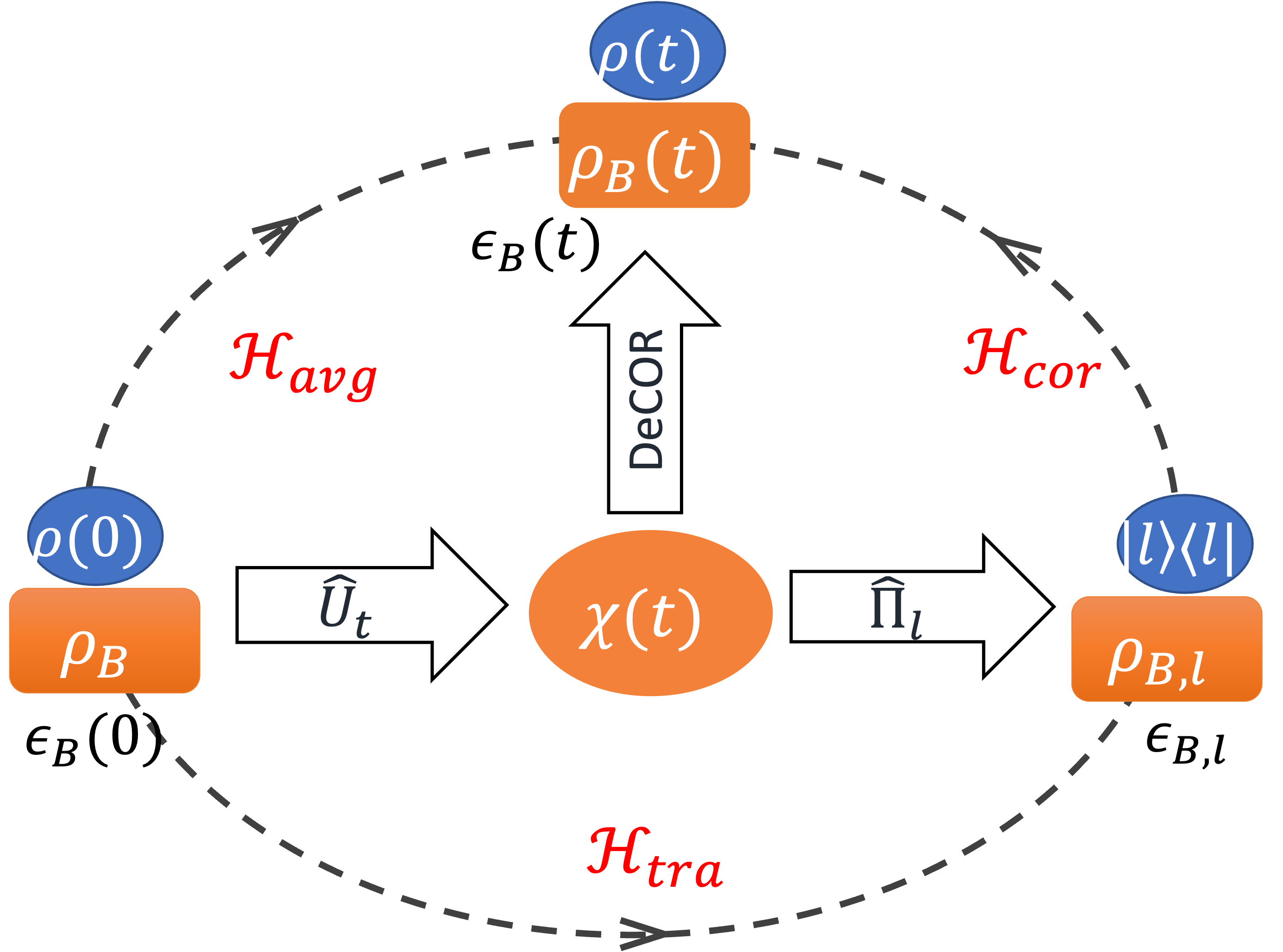
Figure 1: The scheme of temperature estimation. The initial product state $\chi(0)=\rho(0)\otimes\rho_{B}$ evolves to $\chi(t)$ under unitary evolution $\hat{U}_{t}$. A following projection measurement under a properly chosen basis $\hat{\Pi}_{l}=|l\rangle\langle l|$ is applied on the thermometer part, which reduces the sample state to $\rho_{B,l}$ with probability $P_{l}=\text{Tr}[\hat{\Pi}_{l}\chi(t)]$. Sequential measurements on sample’s energy of initial state and final state yields $\epsilon_{B}(0)$ and $\epsilon_{B,l}$, respectively. The difference $\epsilon_{B}(0)-\epsilon_{B,l}$ is defined as the trajectory heat as it depends on the evolution path of the thermometer. The sample’s average energy is measured from the decorrealated state $\rho_{B}(t):=\text{Tr}_{S}[\chi(t)]$, noted as $\epsilon_{B}(t)$. Differences between $\epsilon_{B,l}$ and $\epsilon_{B}(t)$ is defined as the correlation heat as it reflects the difference between the total system under or under not a decorrelation process and the difference $\epsilon_{B}(0)-\epsilon_{B}(t)$ is defined as the average heat.

II temperature-heat UR

Consider a general temperature sensing process. The scheme is illustrated in Fig. 1. The thermometer (denoted as $S$) is prepared to an initial state $\rho(0)$. The sample (denoted as $B$) is in equilibrium state $\rho_{B}=e^{-\beta\hat{H}_{B}}/Z_{B}$, where $\beta=1/K_{B}T$ is the inverse temperature with Boltzmann constant $K_{B}$ and distribution function $Z_{B}$. The thermometer then interacts with the sample and evolves according to the total Hamiltonian

$$\hat{H}=\hat{H}_{S}+\hat{H}_{B}+\hat{H}_{I},$$ (1)

where $\hat{H}_{S}$ is the thermometer’s Hamiltonian and $\hat{H}_{I}$ is thermometer-sample interaction. After a time $t$ evolution, the total system reads $\chi(t)=\hat{U}_{t}\chi(0)\hat{U}^{\dagger}_{t}$ with $\chi(0)=\rho(0)\otimes\rho_{B}$ and $\hat{U}_{t}=e^{-i\hat{H}t/{\hbar}}$. Through this evolution process, the temperature information of the sample is encoded into the thermometer’s state $\rho(t)=\text{Tr}_{B}[\chi(t)]$. Properly choosing the measurement basis $\hat{\Pi}_{l}=|l\rangle\langle l|$, the probability distribution $P_{l}=\text{Tr}[\hat{\Pi}_{l}\chi(t)]$ is obtained from the projection measurements, which is a function of the temperature. Repeat such processes many times, the temperature is estimated from the probability function $P_{l}$ and the precision is limited by the Cramér-Rao bound

$$(\Delta\beta)^{2}\geq 1/(N\mathcal{F}),$$ (2)

where $N$ is the number of the measurements and $\mathcal{F}$ is the Fisher information with the definition

$$\mathcal{F}=\sum_{l}P_{l}\mathcal{L}^{2}_{\beta}.$$ (3)

Here $\mathcal{L}_{\beta}=\frac{d\ln P_{l}}{d(-\beta)}$ is the score function [43]. Note that different measurement basis $\hat{\Pi}_{l}$ can cause different Fisher information and the optimal basis would yield the largest Fisher information $\mathcal{F}_{Q}$, which is known as the quantum fisher information [44].

It is interesting to note that the Fisher information can be interpreted as the fluctuation of the score function, which is, however, an information quantity. Here, we aim to find a physical interpretation of the score function. A detail calculation yields

$$\mathcal{L}_{\beta}=\frac{1}{P_{l}}\text{Tr}[\hat{\Pi}_{l}\hat{U}_{t}\hat{H}_{B}\chi(0)\hat{U}_{t}^{\dagger}]-\text{Tr}[\hat{H}_{B}\rho_{B}].$$ (4)

A clever decomposition shows that $\mathcal{L}_{\beta}$ is the sum of trajectory heat, correlation heat, and average heat, i. e., $\mathcal{L}_{\beta}=\mathcal{H}_{tra}+\mathcal{H}_{cor}-\mathcal{H}_{avg}$ [45]. The detail expressions of these heat terms are

$$\mathcal{H}_{tra} = \frac{1}{P_{l}}\text{Tr}[\hat{\Pi}_{l}(\hat{U}_{t}\hat{H}_{B}\chi(0)\hat{U}_{t}^{\dagger}-\hat{H}_{B}\chi(t))],~{}~{}$$ (5)

$$\mathcal{H}_{cor} = \frac{1}{P_{l}}\text{Tr}[\hat{\Pi}_{l}\hat{H}_{B}\chi(t)]-\text{Tr}[\hat{H}_{B}\rho_{B}(t)],$$ (6)

$$\mathcal{H}_{avg} = \text{Tr}[\hat{H}_{B}\rho_{B}-\hat{H}_{B}\rho_{B}(t)],$$ (7)

where $\rho_{B}(t)=\text{Tr}_{S}[\chi(t)]$. Here we use the term ’heat’ to characterize the change of sample’s energy [46, 47, 48, 49] although there is still controversy regarding how to define heat in a strong coupling system [50, 51]. The physical meaning of these terms is explained via the schematic diagram shown in Fig. 1. Twice sequential measurements of $\hat{H}_{B}$ are applied to the initial and the final states after the projection measurement, yielding the outputs $\epsilon_{B}(0)$ and $\epsilon_{B,l}$, respectively. Their difference is defined as the trajectory heat, i. e., $\mathcal{H}_{tra}=\epsilon_{B}(0)-\epsilon_{B,l}$, which depends on the thermometer’s evolution path from $\rho(0)$ to $|l\rangle\langle l|$. It follows the standard two-point measurements and reflects the loss of sample’s energy along thermometer’s given evolution [47, 48]. The difference between $\epsilon_{B,l}$ and the sample’s energy $\epsilon_{B}(t)$ measured from the decorrealted state $\rho(t)\otimes\rho_{B}(t)$ is defined as the correlation heat, i. e., $\mathcal{H}_{cor}=\epsilon_{B,l}-\epsilon_{B}(t)$. As $\mathcal{H}_{cor}$ quantifies the heat difference under or under not decorrelation process, it characterizes the correlation between the thermometer and the sample. Therefore, we refer to it as the correlation heat. It goes to zero when $\chi(t)$ is a product state, e.g., $\chi(t)\approx\rho(t)\otimes\rho_{B}(t)$. At last, the sample’s energy difference between $\epsilon_{B}(0)$ and $\epsilon_{B}(t)$ is defined as the average heat [49].

By further noting $\mathcal{H}_{avg}=\langle\mathcal{H}_{tra}\rangle$ is the mean of $\mathcal{H}_{tra}$, we get a simple expression of the score

$$\mathcal{L}_{\beta}=\delta\mathcal{H}_{tra}+\mathcal{H}_{cor},$$ (8)

where $\delta\mathcal{H}_{tra}=\mathcal{H}_{tra}-\mathcal{H}_{avg}$. Hereafter, we use $\langle\rangle$ to denote the average over $P_{l}$. Using these results, we find that $\mathcal{F}=\langle(\delta\mathcal{H}_{tra}+\mathcal{H}_{cor})^{2}\rangle$. It is the main result of this paper. It reveals that it is the fluctuation of heat that fundamentally determines the temperature precision, i.e.,

$$\Delta\beta^{2}\langle(\delta\mathcal{H}_{tra}+\mathcal{H}_{cor})^{2}\rangle\geq 1.$$ (9)

Here we set the measurement time $N=1$. As it shares the same expression as the UR, we refer it as the temperature-heat UR in the temperature sensing process. From it, we can identify two resources to enhance temperature precision: one is the ability for heat exchange [28]; the other is the correlation between the thermometer and the sample [18, 19]. In the following section, we illustrate these two types of resources based on specific thermometers.

III heat-exchange thermometer

The first type of thermometer we considered operates through the exchange of excitations or heat [33, 52, 23]. Here, we take a toy model consisting of two coupled oscillators to illustrate this type of quantum thermometry. One oscillator is employed as the thermometer, while the other functions as the thermal sample. Despite its simplicity, this model captures many key features of thermometers working through heat exchange. The Hamiltonians of $\hat{H}_{S}$, $\hat{H}_{B}$, and $\hat{H}_{I}$ read

$$\hat{H}_{S}=\omega_{a}\hat{a}^{\dagger}\hat{a},~{}~{}\hat{H}_{B}=\omega_{0}\hat{b}^{\dagger}\hat{b},~{}~{}\hat{H}_{I}=g(\hat{a}^{\dagger}\hat{b}+\hat{b}^{\dagger}\hat{a}),$$ (10)

where $\hat{a}(\hat{b})$ and $\hat{a}^{\dagger}(\hat{b}^{\dagger})$ are the annihilation and creation operators of the thermometer (sample), respectively, with the characteristic energy $\omega_{a}(\omega_{0})$ and $g$ is the coupling strength. We set the initial state of the thermometer as the vacuum state $\rho(0)=|0_{a}\rangle\langle 0_{a}|$, which is proven to be the optimal for temperature estimation [33].

Set the Fock state $|l_{a}\rangle$ as the measurement basis, which is demonstrated to be the optimal basis for temperature estimation [23]. One can exactly solve this model and get the trajectory heat and the correlation heat. Results are [53]

$$\mathcal{H}_{tra}=l\omega_{0},~{}~{}\mathcal{H}_{cor}=\frac{\bar{n}_{b}-\bar{n}(t)}{1+\bar{n}(t)}\omega_{0}\delta l,$$ (11)

where $\delta l=l-\bar{n}(t)$ with $\bar{n}(t)=\langle l\rangle$ being the mean of $l$ and $\bar{n}_{b}=\frac{1}{e^{\beta\omega_{0}}-1}$ is the average excitation number in the initial state of the sample. Detail calculation yields $\bar{n}(t)=\frac{g^{2}\bar{n}_{b}}{\Delta^{2}+g^{2}}\sin^{2}\sqrt{\Delta^{2}+g^{2}}t$ with $\Delta=(\omega_{a}-\omega_{0})/2$ and the fluctuation $\langle(\delta l)^{2}\rangle=\bar{n}(t)(1+\bar{n}(t))$. Using these results, we obtain

$$\Delta\beta/\beta\geq\frac{1}{(\beta\omega_{0})(1+\bar{n}_{b})}\sqrt{\frac{1+\bar{n}(t)}{\bar{n}(t)}}.$$ (12)

From Eq. (11), its evident that the trajectory heat is directly proportional to the number of excitations absorbed from the sample. To enhance the fluctuation of the trajectory heat, one needs to optimize the heat exchange ability by selecting the optimal evolution time, denoted as $t_{opt}=(i+1/2)\pi/\sqrt{\Delta^{2}+g^{2}}$, where $i\in\mathbb{Z}$ and the optimal detuning, denoted as $\Delta_{opt}=0$. Conversely, a large detuning $\Delta\gg g$ would obstruct the heat exchange, rendering the thermometer inefficient. Additionally, examining the correlation heat in Eq. (11), it is proportional to the difference $\bar{n}_{b}-\bar{n}(t)$. One can attribute this term to the conservation of the total particle number $\hat{N}=\hat{a}^{\dagger}\hat{a}+\hat{b}^{\dagger}\hat{b}$ due to $[\hat{H},\hat{N}]=0$. As the correlation heat shares the same sign with the trajectory heat, it consistently enhances the temperature precision with a factor $(1+\bar{n}(t))/(1+\bar{n}_{b})$ . This enhancement becomes particularly dominant during rapid high-temperature sensing, where $(1+\bar{n}(t))/(1+\bar{n}_{b})\ll 1$. Through this simple example, we demonstrate that the ability to exchange heat is the primary resource for heat-exchange quantum thermometers, and the correlation heat further enhances the temperature precision.

The increase of the heat exchange ability would help us to realize the high-precision quantum thermometer, especially at low-temperature. In low-temperature quantum thermometry, there is an estimation error divergence problem [28] caused by the mismatch between thermometer’s characteristic frequency $\omega_{a}$ and sample’s typical frequency $\omega_{0}\approx K_{B}T$. For a multimode sample, Jørgensen et al. revealed a tight bound $(\Delta\beta/\beta)\sim(\beta)^{(1+s)/2}$ on the finite-resolution quantum thermometry, where the multimode sample is described by the spectral density $J(\omega):=\sum_{k}g_{k}^{2}\delta(\omega-\omega_{k})=\alpha\omega^{s}\omega^{1-s}_{c}e^{-\omega/\omega_{c}}$ with $s\geq 0$ [52]. A single mode approximation yields $g^{2}\approx\int^{K_{B}T}_{0}d\omega J(\omega)\sim(K_{B}T)^{1+s}$ with $\omega_{0}\approx K_{B}T$. It yields the bound $\Delta\beta/\beta\geq\frac{(e^{\beta\omega_{0}}-1)^{3/2}}{\beta\omega_{0}e^{\beta\omega_{0}}}\frac{\Delta}{|g|}\sim\beta^{(1+s)/2}$ according to (12) , which recovers the result in [52]. To address the error divergence issue, one can either reduce the thermometer’s characteristic frequency [54, 20, 23] or enhance the coupling strength [12, 13, 52]. This highlights the importance of quantum criticality, which effectively provides a gapless thermometer, and the strong coupling for low-temperature thermometers.

IV correlation-heat thermometer

There is another type of thermometer that operates based on correlation heat, rather than heat exchange, which we refer to as a correlation-heat thermometer. One typical example is the dephasing thermometer [37, 8, 10, 11], which operates based on the dephasing process. Here, we consider a multimode sample coupled with a two-level thermometer. By setting $\hat{H}_{S}=0$ as it is irrelevant to the dephasing process, the Hamiltonians read

$$\hat{H}_{I}=\hat{\sigma}_{z}\sum_{k}g_{k}(\hat{b}_{k}+\hat{b}_{k}),~{}~{}\hat{H}_{B}=\sum_{k}\omega_{k}\hat{b}^{\dagger}_{k}\hat{b}_{k},$$ (13)

where $\hat{\sigma}_{z}$ is the Pauli matrix, $\hat{b}_{k}$ and $\hat{b}^{\dagger}_{k}$ are the annihilation and creation operators of the $k-$th bosonic mode in the sample, respectively, with characteristic frequency $\omega_{k}$, and $g_{k}$ is the coupling strength.

We set both the initial state and measurement basis to along the $x$-direction, i.e., $\rho(0)=\frac{\mathbb{I}}{2}+\frac{\sigma_{x}}{2}$ and $\hat{\Pi}_{\pm}=|\pm_{x}\rangle\langle\pm_{x}|$. Both the trajectory heat and correlation heat are analytically calculated, leveraging the exact solvability of the system [55]. Results are [53]

$$\mathcal{H}_{tra}=Q-\frac{le^{-\Gamma(t)}}{P_{l}}Q,~{}~{}\mathcal{H}_{cor}=\frac{le^{-\Gamma(t)}}{P_{l}}(Q+C),$$ (14)

where $P_{l}=\frac{1+le^{-\Gamma(t)}}{2}$ with $l=\pm$ is the probability of the thermometer being $|l_{x}\rangle$ state, $Q=-2\sum_{k}\frac{g^{2}_{k}}{\omega_{k}}(1-\cos(\omega_{k}t))$ is the average heat absorbed from the sample, $C=-4\sum_{k}\frac{g^{2}_{k}}{\omega_{k}}\bar{n}_{k}(1+\bar{n}_{k})(1-\cos(\omega_{k}t))$, and the decoherence factor $\Gamma(t)=4\sum_{k}\frac{g^{2}_{k}}{\omega^{2}_{k}}(2\bar{n}_{k}+1)(1-\cos(\omega_{k}t))$ with $\bar{n}_{k}=\frac{1}{e^{\beta\omega_{k}}-1}$.

Equation (14) reveals that there is an average heat $\langle\mathcal{H}_{tra}\rangle=Q$ in the dephasing process, although dephasing is seen as a process without heat exchange. Detail analysis reveals that, rather than the heat exchange, it is the interaction term $\hat{H}_{I}$ that induces the trajectory heat [49]. It is noteworthy that this term does not contribute to determining the temperature due to its fluctuation, denoted as $\delta\mathcal{H}_{tra}=-\frac{1}{P_{l}}le^{-\Gamma(t)}Q$, being cancelled out by the corresponding counter term $\frac{1}{P_{l}}le^{-\Gamma(t)}Q$ in the correlation heat. Thus, it is the correlation heat $\mathcal{H}^{\prime}_{cor}=\frac{1}{P_{l}}le^{-\Gamma(t)}C$ that finally determines the temperature precision in the dephasing thermometer. A simple calculation shows that the temperature precision satisfies

$$\Delta\beta/\beta\geq\sqrt{e^{2\Gamma(t)}-1}/(2\beta|C|).$$ (15)

From it, we can draw the conclusion that the correlation heat is the resource for dephasing thermometers. Enhancing the correlation between the sample and thermometer is essential for achieving precise temperature estimation in this type of thermometers. Setting the dephasing time as $t^{\ast}_{2}$. In low-temperature limit, the temperature precision $(\Delta\beta/\beta)\sim\beta^{1+s}/\alpha\omega^{1-s}_{c}(t^{\ast}_{2})^{2}$ is obtained for the spectral density $J(\omega)=\alpha\omega^{s}\omega^{1-s}_{c}e^{-\omega/\omega_{c}}$ [37, 11]. From it, we can find that the coherence time $t^{\ast}_{2}$ servers as a valuable resource for increasing the correlation heat and thus improving temperature precision.

V temperature-energy UR

Before concluding this manuscript, it is interesting to note that the temperature-heat UR, as shown in Eq. (9), converges to the temperature-energy UR in the steady state limit. Consider the total system is time-independent, it results in the conservation of the total energy. Thus, the change in the sample’s energy is equivalent to the change in the thermometer’s energy plus a modification induced by $\hat{H}_{I}$. According to this conservation law, we have

$$\mathcal{H}_{tra}=\frac{1}{P_{l}}\text{Tr}[\hat{\Pi}_{l}(\hat{H}^{\prime}_{S}\chi(t)-\hat{U}_{t}\hat{H}^{\prime}_{S}\chi(0)\hat{U}^{\dagger}_{t})],$$ (16)

where $\hat{H}^{\prime}_{S}=\hat{H}_{S}+\hat{H}_{I}$. In the steady state limit, the thermometer would relaxes to the equilibrium state $\rho_{s}=\text{Tr}_{B}[\chi_{s}]$ with $\chi_{s}=e^{-\beta\hat{H}}/Z$ being the equilibrium state of the total system [56, 41, 57]. The fluctuation of the internal energy under a projection measurement $\hat{\Pi}_{l}$ is defined as $\delta U=\frac{1}{P_{l}}\text{Tr}[\hat{\Pi}_{l}\frac{d\rho_{s}}{d(-\beta)}]$ according to the definition for a Gibbs state $e^{-\beta\hat{H}^{\ast}_{S}}/Z^{\ast}_{S}$ [41, 57]. The detail expression is

$$\delta U=\frac{1}{P_{l}}\text{Tr}[\hat{\Pi}_{l}(\hat{H}^{\prime}_{S}+\hat{H}_{B})\chi_{s}]-\text{Tr}[(\hat{H}^{\prime}_{S}+\hat{H}_{B})\chi_{s}].$$ (17)

It is exactly the heat term $(\delta\mathcal{H}_{tra}+\mathcal{H}_{cor})$, noting that $\frac{1}{P_{l}}\text{Tr}[\hat{\Pi}_{l}\hat{U}_{t}\hat{H}^{\prime}_{S}\chi(0)\hat{U}^{\dagger}_{t}]-\text{Tr}[\hat{U}_{t}\hat{H}^{\prime}_{S}\chi(0)\hat{U}^{\dagger}_{t}]=0$ in the steady state limit. Thus, the temperature-heat UR shown in Eq. (9) reduces to the temperature-energy UR

$$\Delta\beta\Delta U\geq 1,$$ (18)

where $\Delta U^{2}=\langle(\delta U)^{2}\rangle$. This result not only demonstrates the consistency of the temperature-heat UR in temperature estimation process and the well known temperature-energy UR in thermodynamics but also establishes a connection between the information theory and the thermodynamics.

VI conclusions

In summary, we reveal the temperature-heat uncertainty relation in the temperature estimation process, which puts a fundamental limit for quantum thermometry. We find that the estimation precision is fundamentally determined by the fluctuation of the trajectory heat plus the correlation heat. Based on the two type of thermometers, we demonstrate that both of these heat terms are resources for enhancing temperature precision. By clearly displaying the resources for enhancing temperature precision, our work is helpful for designing high-precision quantum thermometers. Additionally, we demonstrate that the temperature-heat UR converges to the well known temperature-energy UR in the steady state limit. Thus, this result establishes a connection between estimation theory, or information theory, and thermodynamics, which could be valuable for studying quantum thermodynamics in terms of information theory, especially in the strong coupling regime [57].

The work is supported by the National Natural Science Foundation (Grant No. 12047501), Fundamental Research Funds for the Central Universities (Grant No. 561219028), and China Postdoctoral Science Foundation (Grant No. BX20220138 No. 2022M710063).

References

- Puglisi et al. [2017] A. Puglisi, A. Sarracino, and A. Vulpiani, Temperature in and out of equilibrium: A review of concepts, tools and attempts, Phys., Rep. 709-710, 1 (2017).
- Neumann et al. [2013] P. Neumann, I. Jakobi, F. Dolde, C. Burk, R. Reuter, G. Waldherr, J. Honert, T. Wolf, A. Brunner, J. H. Shim, D. Suter, H. Sumiya, J. Isoya, and J. Wrachtrup, High-precision nanoscale temperature sensing using single defects in diamond, Nano Lett. 13, 2738 (2013).
- Kucsko et al. [2013] G. Kucsko, P. C. Maurer, N. Y. Yao, M. Kubo, H. J. Noh, P. K. Lo, H. Park, and M. D. Lukin, Nanometre-scale thermometry in a living cell, Nature 500, 54 (2013).
- Ferreiro-Vila et al. [2021] E. Ferreiro-Vila, J. Molina, L. M. Weituschat, E. Gil-Santos, P. A. Postigo, and D. Ramos, Micro-kelvin resolution at room temperature using nanomechanical thermometry, ACS Omega 6, 23052 (2021).
- Stace [2010] T. M. Stace, Quantum limits of thermometry, Phys. Rev. A 82, 011611 (2010).
- Jevtic et al. [2015] S. Jevtic, D. Newman, T. Rudolph, and T. M. Stace, Single-qubit thermometry, Phys. Rev. A 91, 012331 (2015).
- Mukherjee et al. [2019] V. Mukherjee, A. Zwick, A. Ghosh, X. Chen, and G. Kurizki, Enhanced precision bound of low-temperature quantum thermometry via dynamical control, Commun. Phys. 2, 162 (2019).
- Mitchison et al. [2020] M. T. Mitchison, T. Fogarty, G. Guarnieri, S. Campbell, T. Busch, and J. Goold, In situ thermometry of a cold fermi gas via dephasing impurities, Phys. Rev. Lett. 125, 080402 (2020).
- Zhang and Tong [2022] D.-J. Zhang and D. M. Tong, Approaching heisenberg-scalable thermometry with built-in robustness against noise, npj Quantum Inf. 8, 81 (2022).
- Adam et al. [2022] D. Adam, Q. Bouton, J. Nettersheim, S. Burgardt, and A. Widera, Coherent and dephasing spectroscopy for single-impurity probing of an ultracold bath, Phys. Rev. Lett. 129, 120404 (2022).
- Yuan et al. [2023] J.-B. Yuan, B. Zhang, Y.-J. Song, S.-Q. Tang, X.-W. Wang, and L.-M. Kuang, Quantum sensing of temperature close to absolute zero in a bose-einstein condensate, Phys. Rev. A 107, 063317 (2023).
- Correa et al. [2017] L. A. Correa, M. Perarnau-Llobet, K. V. Hovhannisyan, S. Hernández-Santana, M. Mehboudi, and A. Sanpera, Enhancement of low-temperature thermometry by strong coupling, Phys. Rev. A 96, 062103 (2017).
- Mehboudi et al. [2019a] M. Mehboudi, A. Lampo, C. Charalambous, L. A. Correa, M. A. García-March, and M. Lewenstein, Using polarons for sub-nk quantum nondemolition thermometry in a bose-einstein condensate, Phys. Rev. Lett. 122, 030403 (2019a).
- Zhang and Wu [2021] Z.-Z. Zhang and W. Wu, Non-markovian temperature sensing, Phys. Rev. Res. 3, 043039 (2021).
- Mihailescu et al. [2023] G. Mihailescu, S. Campbell, and A. K. Mitchell, Thermometry of strongly correlated fermionic quantum systems using impurity probes, Phys. Rev. A 107, 042614 (2023).
- Brenes and Segal [2023] M. Brenes and D. Segal, Multispin probes for thermometry in the strong-coupling regime, Phys. Rev. A 108, 032220 (2023).
- Xu et al. [2023] L. Xu, J.-B. Yuan, S.-Q. Tang, W. Wu, Q.-S. Tan, and L.-M. Kuang, Non-markovian enhanced temperature sensing in a dipolar bose-einstein condensate, Phys. Rev. A 108, 022608 (2023).
- Seah et al. [2019] S. Seah, S. Nimmrichter, D. Grimmer, J. P. Santos, V. Scarani, and G. T. Landi, Collisional quantum thermometry, Phys. Rev. Lett. 123, 180602 (2019).
- Planella et al. [2022] G. Planella, M. F. B. Cenni, A. Acín, and M. Mehboudi, Bath-induced correlations enhance thermometry precision at low temperatures, Phys. Rev. Lett. 128, 040502 (2022).
- Hovhannisyan and Correa [2018] K. V. Hovhannisyan and L. A. Correa, Measuring the temperature of cold many-body quantum systems, Phys. Rev. B 98, 045101 (2018).
- Mirkhalaf et al. [2021] S. S. Mirkhalaf, D. Benedicto Orenes, M. W. Mitchell, and E. Witkowska, Criticality-enhanced quantum sensing in ferromagnetic bose-einstein condensates: Role of readout measurement and detection noise, Phys. Rev. A 103, 023317 (2021).
- Aybar et al. [2022] E. Aybar, A. Niezgoda, S. S. Mirkhalaf, M. W. Mitchell, D. Benedicto Orenes, and E. Witkowska, Critical quantum thermometry and its feasibility in spin systems, Quantum 6, 808 (2022).
- Zhang et al. [2022a] N. Zhang, C. Chen, S.-Y. Bai, W. Wu, and J.-H. An, Non-markovian quantum thermometry, Phys. Rev. Appl. 17, 034073 (2022a).
- Giazotto et al. [2006] F. Giazotto, T. T. Heikkilä, A. Luukanen, A. M. Savin, and J. P. Pekola, Opportunities for mesoscopics in thermometry and refrigeration: Physics and applications, Rev. Mod. Phys. 78, 217 (2006).
- Hofer et al. [2017] P. P. Hofer, J. B. Brask, M. Perarnau-Llobet, and N. Brunner, Quantum thermal machine as a thermometer, Phys. Rev. Lett. 119, 090603 (2017).
- De Pasquale and Stace [2018] A. De Pasquale and T. M. Stace, Quantum thermometry, in Thermodynamics in the Quantum Regime: Fundamental Aspects and New Directions, edited by F. Binder, L. A. Correa, C. Gogolin, J. Anders, and G. Adesso (Springer International Publishing, Cham, 2018) pp. 503–527.
- Mehboudi et al. [2019b] M. Mehboudi, A. Sanpera, and L. A. Correa, Thermometry in the quantum regime: recent theoretical progress, J. Phys. A 52, 303001 (2019b).
- Potts et al. [2019] P. P. Potts, J. B. Brask, and N. Brunner, Fundamental limits on low-temperature quantum thermometry with finite resolution, Quantum 3, 161 (2019).
- Rubio et al. [2021] J. Rubio, J. Anders, and L. A. Correa, Global quantum thermometry, Phys. Rev. Lett. 127, 190402 (2021).
- Mehboudi et al. [2022] M. Mehboudi, M. R. Jørgensen, S. Seah, J. B. Brask, J. Kołodyński, and M. Perarnau-Llobet, Fundamental limits in bayesian thermometry and attainability via adaptive strategies, Phys. Rev. Lett. 128, 130502 (2022).
- Escher et al. [2011] B. M. Escher, R. L. de Matos Filho, and L. Davidovich, General framework for estimating the ultimate precision limit in noisy quantum-enhanced metrology, Nature Physics 7, 406 (2011).
- Giovannetti et al. [2011] V. Giovannetti, S. Lloyd, and L. Maccone, Advances in quantum metrology, Nature Photonics 5, 222 (2011).
- Correa et al. [2015] L. A. Correa, M. Mehboudi, G. Adesso, and A. Sanpera, Individual quantum probes for optimal thermometry, Phys. Rev. Lett. 114, 220405 (2015).
- De Pasquale et al. [2016] A. De Pasquale, D. Rossini, R. Fazio, and V. Giovannetti, Local quantum thermal susceptibility, Nat. Commun. 7, 12782 (2016).
- Hovhannisyan et al. [2021] K. V. Hovhannisyan, M. R. Jørgensen, G. T. Landi, A. M. Alhambra, J. B. Brask, and M. Perarnau-Llobet, Optimal quantum thermometry with coarse-grained measurements, PRX Quantum 2, 020322 (2021).
- Cavina et al. [2018] V. Cavina, L. Mancino, A. De Pasquale, I. Gianani, M. Sbroscia, R. I. Booth, E. Roccia, R. Raimondi, V. Giovannetti, and M. Barbieri, Bridging thermodynamics and metrology in nonequilibrium quantum thermometry, Phys. Rev. A 98, 050101 (2018).
- Razavian et al. [2019] S. Razavian, C. Benedetti, M. Bina, Y. Akbari-Kourbolagh, and M. G. A. Paris, Quantum thermometry by single-qubit dephasing, Eur. Phys. J. Plus 134, 284 (2019).
- Bouton et al. [2020] Q. Bouton, J. Nettersheim, D. Adam, F. Schmidt, D. Mayer, T. Lausch, E. Tiemann, and A. Widera, Single-atom quantum probes for ultracold gases boosted by nonequilibrium spin dynamics, Phys. Rev. X 10, 011018 (2020).
- Landau and Lifshitz [1980] L. D. Landau and E. M. Lifshitz, Statistical Physics. (Pergamon Press, Oxford, 1980).
- Paris [2015a] M. G. A. Paris, Achieving the landau bound to precision of quantum thermometry in systems with vanishing gap, J. Phys. A: Math. Theor. 49, 03LT02 (2015a).
- Miller and Anders [2018] H. J. D. Miller and J. Anders, Energy-temperature uncertainty relation in quantum thermodynamics, Nat. Commun. 9, 2203 (2018).
- Coles et al. [2017] P. J. Coles, M. Berta, M. Tomamichel, and S. Wehner, Entropic uncertainty relations and their applications, Rev. Mod. Phys. 89, 015002 (2017).
- Fisher [1925] R. A. Fisher, Theory of statistical estimation, Math. Proc. Cambridge Philos. Soc. 22, 700–725 (1925).
- Braunstein and Caves [1994] S. L. Braunstein and C. M. Caves, Statistical distance and the geometry of quantum states, Phys. Rev. Lett. 72, 3439 (1994).
- Zhang et al. [2022b] N. Zhang, S.-Y. Bai, and C. Chen, Temperature uncertainty relation in non-equilibrium thermodynamics (2022b), arXiv:2204.10044 .
- Goold et al. [2014] J. Goold, U. Poschinger, and K. Modi, Measuring the heat exchange of a quantum process, Phys. Rev. E 90, 020101 (2014).
- Funo and Quan [2018] K. Funo and H. T. Quan, Path integral approach to heat in quantum thermodynamics, Phys. Rev. E 98, 012113 (2018).
- Aurell [2018] E. Aurell, Characteristic functions of quantum heat with baths at different temperatures, Phys. Rev. E 97, 062117 (2018).
- Popovic et al. [2021] M. Popovic, M. T. Mitchison, A. Strathearn, B. W. Lovett, J. Goold, and P. R. Eastham, Quantum heat statistics with time-evolving matrix product operators, PRX Quantum 2, 020338 (2021).
- Seifert [2016] U. Seifert, First and second law of thermodynamics at strong coupling, Phys. Rev. Lett. 116, 020601 (2016).
- Talkner and Hänggi [2016] P. Talkner and P. Hänggi, Open system trajectories specify fluctuating work but not heat, Phys. Rev. E 94, 022143 (2016).
- Jørgensen et al. [2020] M. R. Jørgensen, P. P. Potts, M. G. A. Paris, and J. B. Brask, Tight bound on finite-resolution quantum thermometry at low temperatures, Phys. Rev. Res. 2, 033394 (2020).
- [53] See the Supplemental Material for detail calculations for (A) heat-exchange thermometer; (B) dephasing thermometer.
- Paris [2015b] M. G. A. Paris, Achieving the landau bound to precision of quantum thermometry in systems with vanishing gap, J. Phys. A: Math. Theor. 49, 03LT02 (2015b).
- Breuer and Petruccione [2007] H.-P. Breuer and F. Petruccione, The Theory of Open Quantum Systems (Oxford University Press, 2007).
- Jarzynski [2004] C. Jarzynski, Nonequilibrium work theorem for a system strongly coupled to a thermal environment, J. Stat. Mech. Theory Exp. 2004, P09005 (2004).
- Talkner and Hänggi [2020] P. Talkner and P. Hänggi, Colloquium: Statistical mechanics and thermodynamics at strong coupling: Quantum and classical, Rev. Mod. Phys. 92, 041002 (2020).