Dynamic gain and frequency comb formation in exceptional-point lasers
Abstract
Exceptional points (EPs)—singularities in the parameter space of non-Hermitian systems where two nearby eigenmodes coalesce—feature unique properties with applications for microcavity lasers such as sensitivity enhancement and chiral emission. Present EP lasers operate with static populations in the gain medium. Here, we show theoretically that a laser operating sufficiently close to an EP will spontaneously induce a multi-spectral multi-modal instability that creates an oscillating population inversion and generates a frequency comb. The comb formation is enhanced by the non-orthogonality of modes via the Petermann factor. Such an “EP comb” features an ultra-compact size and a widely tunable repetition rate, without requiring external modulators or a continuous-wave pump. We develop an exact ab initio dynamic solution of the space-dependent Maxwell–Bloch equations, describing all steady-state properties of the EP comb. We illustrate this phenomenon in a realistic parity-time-symmetric 5-µm-long AlGaAs cavity and validate our prediction with finite-difference time-domain simulations. This work reveals the rich physics that connect non-Hermitian degeneracies and the nonlinear dynamics of gain media to fundamentally alter the laser behavior.
I Introduction
An exceptional point (EP) is a non-Hermitian degeneracy where not only do two eigenvalues coincide, but the spatial profiles of the two modes also become identical 1, 2, 3, 4, 5. Realizing such non-Hermitian phenomena necessitates gain and loss, making microcavity lasers a fertile ground to explore EPs. The mode coalescence and the unique topology of its eigenvalue landscape enable EP lasers to exhibit counter-intuitive properties such as reversed pump dependence 6, loss-induced lasing 7, and topological state transfer 8, with applications including single-mode operation 9, 10, sensitivity enhancement 11, 12, 13, 14, 15, and chiral emission 16, 17, 18. Optical gain is intrinsically nonlinear, and EP lasers have been modeled 6, 19, 20, 21, 22, 23 by treating the population inversion of the gain medium as time-invariant (called the stationary-inversion approximation; SIA) 24. This approximation is valid for steady-state single-mode lasing and for multi-mode lasing with a frequency separation much larger than the relaxation rate of the population inversion ( ns-1 for semiconductor gain media). Present studies of EP lasers stay in the stationary-inversion regime (Fig. 1a–b). However, sufficiently close to an EP, the frequency separation (i.e., the difference in the real parts of the eigenvalues) between the two modes becomes small enough that the SIA always breaks down. Efforts to extend the existing steady-state laser theory beyond the SIA through perturbative analysis 25, 26 or a time-domain description 27 have not succeeded in describing the nonlinear dynamics of the system close to an EP.
A seemingly unrelated subject is the study of optical frequency combs: lasers with equally spaced spectral lines 28, 29. Initially developed for high-precision frequency-time metrology 30, 31, frequency combs have broad applications in spectroscopy 32, imaging 33, optical 34 and 5G 35 communication, ranging 36, 37 and autonomous driving 38, and machine learning 39, 40, 41. Traditionally, frequency combs are realized through mode-locked lasers, where a periodic modulation of the cavity loss promotes pulse formation 42. More recent approaches include parametric frequency conversion via the Kerr nonlinearity using a continuous-wave (CW) laser and a high-quality-factor microresonator 43, 44, passing a CW laser through electro-optic modulators 45, and using tailored quantum well gain media found in quantum cascade lasers 46, 47. The repetition rate (namely, the comb tooth spacing) of the frequency comb is an important characteristic, and it typically follows the cavity’s free spectral range (FSR).

Here, we show that EP lasers and frequency combs are inherently intertwined concepts: close to an EP, the SIA necessarily breaks down at a gain threshold, above which oscillations in the gain populations emerge, coupling different frequencies and generating a frequency comb (Fig. 1c). This comb threshold does not correspond to an isolated resonance receiving enough gain to overcome its loss as in conventional lasers 48, 49, 50, 51; rather, it stems from the growth of a multi-spectral multi-modal perturbation that induces a dynamic gain balancing the spatial holes of the static gain. Through the Maxwell–Bloch equations, we identify three ingredients that promote comb formation with a dynamic gain: a small frequency separation between two modes, resonance enhancement, and a large Petermann factor 52, 53. The Petermann factor quantifies the non-orthogonality of eigenmodes induced by non-Hermiticity, and it diverges near an EP 54, 55, 56, 57, 58, 59 due to the two-mode coalescence there 1, 2. Therefore, an EP uniquely offers all three ingredients. Thanks to the resonance enhancement and large Petermann factor, we find that an EP with can already induce a strong frequency comb. Distinct from existing types of frequency combs, the repetition rate of such an “EP comb” is unrelated to the cavity’s FSR, enabling an ultra-compact cavity size and a variable repetition rate. It also does not require an external modulator or an external CW laser. We develop an exact dynamic solution of the Maxwell–Bloch equations free of SIA and show the existence of an EP comb in an AlGaAs gain-loss coupled cavity that is merely 5 µm long, producing a comb centered around wavelength 820 nm with a continuously tunable repetition rate between 20 GHz and 27 GHz. The predictions are validated by direct finite-difference time-domain (FDTD) simulations. The rich nonlinear dynamics inherently possible in gain media mediates this unexpected link between non-Hermitian photonics and frequency combs.
II Onset of dynamic inversion and frequency coupling
We start by analyzing the mechanism of EP comb formation. To rigorously describe the spatiotemporal dynamics of an EP laser, we consider the semi-classical Maxwell–Bloch (MB) equations 60, 61:
| (1) | ||||
| (2) | ||||
| (3) |
The MB equations couple the electrical field governed by Maxwell’s equations to the population inversion of the gain medium and the resulting polarization density described by the quantum mechanical density matrix (Supplementary Sec. 1). The , , and here have been normalized to be dimensionless quantities in the units of , , and , respectively, with being the amplitude of the atomic dipole moment, the vacuum permittivity, the Planck constant, and the dephasing rate of the gain-induced polarization (i.e., the bandwidth of the gain). Here, is the normalized net pumping strength and profile, is the frequency gap between the two atomic levels providing population inversion, is the unit vector of the atomic dipole moment with , is the relative permittivity profile of the cold cavity, is a conductivity profile that produces absorption loss, and is the vacuum speed of light. and satisfy an outgoing boundary condition outside the cavity. Note that the light-matter interactions in Eqs. (1)–(2) are nonlinear. The MB equations here are written for a two-level gain medium but can be generalized to multi-level gain 62 and semiconductor gain 63, 61, 64 media.
When the pumping strength reaches the first lasing threshold , the gain overcomes the radiation loss and absorption loss of a cavity resonance, and a single-mode steady-state lasing solution emerges with (Supplementary Sec. 2)
| (4) |
Here, is an effective intensity-dependent and frequency-dependent permittivity profile of the active cavity, , and is the saturated gain. This stationary gain is depleted at locations with strong field intensity, referred to as spatial hole burning. In this single-mode regime, Eq. (4) is an exact solution of the MB equations, the inversion is static, and the gain relaxation rate plays no role at steady state. With the gain in fixed, is an eigenmode of the active cavity with an outgoing boundary condition. In other words, is one of the resonances (also called quasinormal modes 65) of —a special one whose eigenvalue is real instead of complex-valued. Since outgoing waves are produced in the absence of incident waves, the lasing frequency is a pole of the scattering matrix 50, 51.
Further increase of the pump strength will eventually bring the system to the next threshold . In a static laser, is where another resonance of now has enough gain to overcome its loss, corresponding to another pole of the scattering matrix that rises up in the complex-frequency plane to reach the real-frequency axis with a steady-state oscillation 50, 51. While this isolated-resonance picture is intuitive, it neglects the possible dynamics of the gain medium. The second threshold may, in principle, correspond to the onset of a dynamic inversion instead. A dynamic inversion can couple different frequencies, and a coherent superposition of resonances—not an individual one—may exhibit spatiotemporal dynamics that amplify through the collective (static plus dynamic) gain.
To analyze the onset and the effects of a dynamic gain, we first consider a monochromatic perturbation (dashed line in Fig. 1b) to single-mode operation, so the total field is . The frequency difference can be positive or negative. With the inversion almost static, it follows from Eq. (2) that with for , where and . With Eq. (1), we see that the inversion is no longer stationary; as illustrated in Fig. 1b, the perturbation induces a dynamic inversion with
| (5) |
Since this oscillating gain arises from beating in the cross terms of Eq. (1), it is enhanced where and spatially overlap, balancing the hole burning in .
It is commonly assumed 24, 25, 51, 66, 67 that the SIA is valid when , where the beat notes of oscillate so fast that they average away before the gain medium can respond. Indeed, the ratio in Eq. (5) is roughly proportional to . However, the quantity of interest is , not the inversion itself. So, we proceed to analyze how this dynamic inversion affects the light field. Substituting Eq. (5) into Eq. (2) yields an extra polarization component at new frequency with , which drives the system [Eq. (3)] as
| (6) |
The oscillating inversion creates on the right-hand side, which acts like an effective current source oscillating at frequency to produce (Fig. 1b). In Supplementary Sec. 3, we solve Eq. (6) for the dominant contribution of to obtain
| (7) |
We call the “dynamic inversion factor” since it quantifies how the gain dynamics can couple multiple frequencies in a four-wave-mixing fashion. Here, = denotes integration over space, is the eigen frequency of the resonance of that is closest to , and is the spatial profile of that resonance. The new frequency component is enhanced by the spatial overlap between , , and . Note that this factor is proportional to the square of the lasing intensity in but independent of the perturbation strength. So, even for a small perturbation with , and , , and are all proportional to . We also emphasize that in the derivation above, we did not put any restriction on the perturbation. The perturbation can be any superposition (and can include the lasing resonance ), though a transient perturbation will sustain longer if it consists mainly of the long-lived resonances of .
Factor I of captures the well-known ratio , which is typically small. Factor II comes from resonant excitation: when the frequency of the dynamic source in Eq. (6) is close to that of a cavity resonance, the response is enhanced. For a resonant perturbation in a system near an EP, the resonance closest to is with , and the resulting factor II of can boost the dynamic effects to invalidate the SIA even when . Resonant excitation also contributes to the numerator of Factor III through the overlap between the source profile and the resonance profile .
Notably, factor III is additionally enhanced by the Petermann factor of the resonance , in the same manner as how the non-orthogonality of modes enhances the laser linewidth 52, 53. Near an EP, , and mode coalescence 1, 2 makes diverge 54, 55, 56, 57, 58, 59. A Hermitian degeneracy and a non-Hermitian degeneracy both enhance factors I and II. But only an EP has a divergent , uniquely enhancing all contributions I, II, and III of the dynamic inversion factor .
We now know how a dynamic gain couples frequencies, but the preceding analysis does not specify when such a perturbation can materialize into self-sustained steady-state oscillation. In Supplementary Sec. 4, we perform a stability analysis 66, 67 on the single-mode solution Eq. (4), which predicts the decay or growth rate of the perturbation, yielding the second gain threshold . When the dynamic inversion factor is negligible, only the term contributes to the perturbation; this reduces to the conventional isolated-resonance description 50, 51 when . Sufficiently close to an EP, is substantial, so , , and jointly contribute to a dynamic multi-spectral perturbation, and is a superposition of multiple resonances. At threshold , the multi-spectral perturbation has enough gain to overcome its loss, and two new frequencies simultaneously emerge as steady-state oscillations. With a further increase of the pump, the new frequencies generate higher harmonics in the population inversion, with the process cascading down to produce a spectrum of equally-spaced comb lines (Fig. 1c). So, when is sizable, is also the threshold for frequency comb generation and marks the onset of dynamic inversion.
III Exact dynamic solution: P-SALT
With pump beyond the comb threshold , a perturbative analysis is no longer sufficient; instead, one must capture the spatiotemporal dynamics of the system self-consistently. Here, we provide an ab initio formalism to do so. Since the cascade process described above couples frequencies separated by , we postulate a spatiotemporal dependence of the form
| (8) | ||||
| (9) | ||||
| (10) |
with , , and being real numbers. This ansatz is also motivated by the fact that dynamic processes in nonlinear systems often evolve into a closed trajectory called a “limit cycle” 68, which is periodic in time and therefore represented by a Fourier series. The temporal periodicity is .
We show in Supplementary Sec. 5 that the ansatz of Eqs. (8)–(10) forms an exact solution of the MB equations, Eqs. (1)–(3), with no approximation. Eliminating the gain-induced polarization yields a nonlinear equation for the electric field and the population inversion,
| (11) | ||||
| (12) | ||||
with . Different frequency components are coherently coupled through a dynamic inversion oscillating at the frequency difference. Here, and are column vectors with elements and , where is the Kronecker delta with and ; is the identity matrix; is a full matrix with elements ; † denotes matrix conjugate transpose; and are diagonal matrices with and , where was defined earlier.
Solving Eqs. (11)–(12) for , , , and yields all steady-state properties of the laser comb, including the frequency spectrum, temporal dynamics, spatial profiles, and input-output curves. To match the number of equations and the number of unknowns, we recognize that when is a solution, with any real-valued and is also a solution. We name Eqs. (8)–(12) as “periodic-inversion steady-state ab initio laser theory” (P-SALT) and refer to the existing stationary-inversion formalism 48, 49, 50, 51 as SIA-SALT.
IV Exceptional point frequency comb
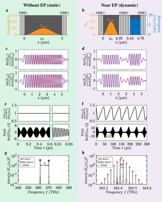
We now use full-wave examples to illustrate the laser dynamics. We start with a typical laser with a static gain operating in the two-mode regime. Consider an AlGaAs gain medium (refractive index 69, gain center nm, gain width s-1, and relaxation rate s-1) 63 with cavity length µm, sandwiched between two distributed Bragg reflector (DBR) partial mirrors and pumped with a smooth profile (Fig. 2a). The system is homogeneous in the transverse directions ( and ), so it reduces to a 1D problem with . At pumping strength , two modes that differ by one longitudinal order lase (Fig. 2c) and produce a sinusoidal beating pattern (Fig. 2e). The frequency separation rad/s equals the FSR of the cavity and is over four orders of magnitude greater than , leading to a negligible dynamic inversion factor . The Petermann factor is here; the gain only balances the radiation loss and does not introduce mode non-orthogonality. The steady-state population inversion is stationary (Fig. 2e), and only two peaks appear in the spectrum (Fig. 2g). For a static laser like this, P-SALT reduces to SIA-SALT.
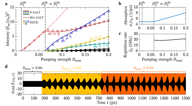
Next, we consider a laser operating close to an EP. We adopt a parity-time-symmetric configuration 3, 4, 70, dividing the cavity into two with a middle DBR (Fig. 2b). One cavity has the same AlGaAs gain with pumping. The other cavity consists of passive GaAs () 69 with a material absorption characterized by conductivity . The coupling and the gain-loss difference are ingredients for an EP. By tuning the cavity lengths and absorption while ramping up the pump (parameters listed in Supplementary Sec. 6), we bring this system close to a linear EP at the first threshold with a Petermann factor of . The near degeneracy reduces the frequency separation to rad/s, well below the cavity FSR. This is still two orders of magnitude greater than s-1, but with the Petermann factor and resonant enhancement, it produces a sizable dynamic inversion factor at the second threshold predicted by the stability analysis of Supplementary Sec. 4. At , a frequency comb emerges (Fig. 2h) despite having only two cold-cavity modes (one per cavity) under the gain curve , accompanied by an oscillating population inversion and a non-sinusoidal beating pattern (Fig. 2f). The spatial profiles at different frequencies are almost identical (Fig. 2d), confirming mode coalescence. The field profiles and gain profiles at all frequencies are shown in Supplementary Sec. 6. Figure 3a shows the evolution of intensity at different frequencies with increasing pump. To stay close to an EP with a small , we maintain the parity-time-symmetric configuration by raising the absorption level when (Fig. 3b–c).
If the gain inversion were to stay stationary, this EP laser would operate only with a single mode because (1) increased gain-loss contrast pushes the second resonance into the lossy region and further away from the threshold to lase 9, 10 and (2) the second resonance shares a similar spatial profile as the lasing one, so its net gain is capped by spatial hole burning. In the present system, SIA-SALT, which assumes a stationary inversion, incorrectly predicts the laser to stay single-mode until an extremely large pump of (red dashed line in Fig. 3a), over 500 times larger than the actual threshold . Given the substantial dynamic inversion factor here, the multi-spectral multi-resonance perturbation described in Sec. II and Fig. 1b can utilize the dynamic gain (which has maximal amplitudes at the spatial holes of the static gain) to amplify, even when the static gain is insufficient for a single resonance to amplify.
EPs feature a boosted sensitivity 11, 12, 13, 14, 15, which unfortunately also amplifies the numerical error, requiring an unusually high accuracy when solving Eqs. (11)–(12). We find finite-difference discretization 51 and the threshold constant-flux basis 50 to both underperform, requiring a very large basis to reach the desired accuracy. For better efficiency, here we solve Eqs. (11)–(12) through a volume integral equation, employing accurate semi-analytic Green’s function of the passive system (Supplementary Sec. 7).
To validate our prediction and to verify the stability of the comb solution, we additionally carry out direct integration of the MB equations using FDTD, where we evolve the system until steady state is reached (Supplementary Sec. 8). To attain sufficient accuracy near an EP, we use a very fine spatial discretization with grid size nm. With a time step size of , this requires over one billion time steps to evolve the system by just one relaxation time ns of the gain medium. The time-consuming FDTD simulations agree quantitatively with all of the P-SALT predictions (Figs. 2–3). Further reducing can bring the agreement even closer while incurring higher computing costs. Figure 3d shows the field evolution in FDTD when the pump is raised across the comb threshold.
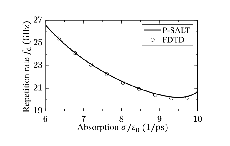
Since the EP comb repetition rate is not tied to the cavity FSR, we can adjust it freely, for example by tuning the material absorption as shown in Fig. 4. This is not possible with mode-locked combs, Kerr combs, and quantum cascade laser combs.
V Discussion
This work predicts how an EP laser can induce dynamics in the gain medium and fundamentally change the laser behavior. It also presents a new route toward frequency comb generation, featuring an ultra-compact cavity size, self-starting operation with no need for an external modulator or CW laser, and a continuously tunable repetition rate decoupled from the cavity’s FSR. This phenomenon bridges the subjects of non-Hermitian photonics, laser physics, nonlinear dynamics, and frequency combs.
The resonance enhancement and Petermann-factor enhancement in the dynamic inversion factor are important. Many lasers have linewidths greater than , so dynamic effects would be blurred by the noise if were a requirement. The resonance and Petermann effects enable EP combs with , making experimental realization much more viable. Prior experiments on EP lasers did not have a small enough frequency difference to enter the dynamic inversion regime with a large enough factor. Realizing an EP comb requires a scheme where the parameters can be tuned with enough precision to reach a sufficient while maintaining the laser linewidth below .
The linewidth of the EP comb will be a subject of future investigation. The divergent Petermann factor is known to broaden the laser linewidth 52, 53, 58, 59, 71. However, existing theories cannot describe the noise of an EP comb. The spontaneous emission is tied to the atomic population, while previous noise analysis either assumes a linear gain 56, 72 or a stationary inversion 73, 53, 74, 59, 23. Additionally, the relation between noise and atomic populations was derived at a local thermal equilibrium 73, 53, which is no longer reached when the inversion fluctuates faster than the spontaneous emission rate. Future work can study the interplay between the linewidth and the dynamics of the gain medium inherent in an EP comb.
A dynamic gain may also lead to interesting phenomena like bistability, hysteresis, period doubling, and the possible onset of chaos. We can expect even richer behaviors near higher-order EPs and in the presence of other forms of nonlinearities.
Finally, we note that the P-SALT formalism here is not limited to EP combs. For example, one may generalize P-SALT to include an external modulation or a saturable absorber to describe the spatiotemporal dynamics of active and passive mode locking.
Acknowledgments: We thank M. Khajavikhan, A. D. Stone, S. G. Johnson, and M. Yu for helpful discussions. This work was supported by the National Science Foundation CAREER award (ECCS-2146021) and the University of Southern California. A.C. acknowledges support from the Laboratory Directed Research and Development program at Sandia National Laboratories. This work was performed, in part, at the Center for Integrated Nanotechnologies, an Office of Science User Facility operated for the U.S. Department of Energy (DOE) Office of Science. Sandia National Laboratories is a multimission laboratory managed and operated by National Technology & Engineering Solutions of Sandia, LLC, a wholly owned subsidiary of Honeywell International, Inc., for the U.S. DOE’s National Nuclear Security Administration under contract DE-NA-0003525. The views expressed in the article do not necessarily represent the views of the U.S. DOE or the United States Government.
Author contributions: X.G. developed the theory on the factor, stability analysis, P-SALT, integral equation solver, and performed the SIA-SALT and P-SALT calculations. X.G., C.W.H., and H.H. analyzed the data. H.H. and A.C. developed the FDTD code. X.G., H.H., and S.S. performed the FDTD simulations. C.W.H. conceived the project and supervised research. C.W.H. and X.G. wrote the paper with inputs from the other coauthors. All authors discussed the results.
Competing interests: The authors declare no competing interests.
References
- [1] Moiseyev, N. Non-Hermitian Quantum Mechanics (Cambridge University Press, 2011).
- [2] Heiss, W. D. The physics of exceptional points. J. Phys. A: Math. Theor. 45, 444016 (2012).
- [3] Feng, L., El-Ganainy, R. & Ge, L. Non-Hermitian photonics based on parity–time symmetry. Nat. Photonics 11, 752–762 (2017).
- [4] El-Ganainy, R. et al. Non-Hermitian physics and PT symmetry. Nat. Phys. 14, 11–19 (2018).
- [5] Miri, M.-A. & Alù, A. Exceptional points in optics and photonics. Science 363, eaar7709 (2019).
- [6] Liertzer, M. et al. Pump-induced exceptional points in lasers. Phys. Rev. Lett. 108, 173901 (2012).
- [7] Peng, B. et al. Loss-induced suppression and revival of lasing. Science 346, 328–332 (2014).
- [8] Schumer, A. et al. Topological modes in a laser cavity through exceptional state transfer. Science 375, 884–888 (2022).
- [9] Feng, L., Wong, Z. J., Ma, R.-M., Wang, Y. & Zhang, X. Single-mode laser by parity-time symmetry breaking. Science 346, 972–975 (2014).
- [10] Hodaei, H., Miri, M.-A., Heinrich, M., Christodoulides, D. N. & Khajavikhan, M. Parity-time–symmetric microring lasers. Science 346, 975–978 (2014).
- [11] Chen, W., Kaya Özdemir, Ş., Zhao, G., Wiersig, J. & Yang, L. Exceptional points enhance sensing in an optical microcavity. Nature 548, 192–196 (2017).
- [12] Hodaei, H. et al. Enhanced sensitivity at higher-order exceptional points. Nature 548, 187–191 (2017).
- [13] Hokmabadi, M. P., Schumer, A., Christodoulides, D. N. & Khajavikhan, M. Non-Hermitian ring laser gyroscopes with enhanced Sagnac sensitivity. Nature 576, 70–74 (2019).
- [14] Lai, Y.-H., Lu, Y.-K., Suh, M.-G., Yuan, Z. & Vahala, K. Observation of the exceptional-point-enhanced Sagnac effect. Nature 576, 65–69 (2019).
- [15] Kononchuk, R., Cai, J., Ellis, F., Thevamaran, R. & Kottos, T. Exceptional-point-based accelerometers with enhanced signal-to-noise ratio. Nature 607, 697–702 (2022).
- [16] Peng, B. et al. Chiral modes and directional lasing at exceptional points. Proc. Natl. Acad. Sci. U.S.A. 113, 6845–6850 (2016).
- [17] Miao, P. et al. Orbital angular momentum microlaser. Science 353, 464–467 (2016).
- [18] Zhang, Z. et al. Tunable topological charge vortex microlaser. Science 368, 760–763 (2020).
- [19] Horstman, L., Hsu, N., Hendrie, J., Smith, D. & Diels, J.-C. Exceptional points and the ring laser gyroscope. Photon. Res. 8, 252–256 (2020).
- [20] Bai, K. et al. Nonlinearity-enabled higher-order exceptional singularities with ultra-enhanced signal-to-noise ratio. Natl. Sci. Rev. 10, nwac259 (2022).
- [21] Benzaouia, M., Stone, A. D. & Johnson, S. G. Nonlinear exceptional-point lasing with ab initio Maxwell–Bloch theory. APL Photonics 7, 121303 (2022).
- [22] Ji, K. et al. Tracking exceptional points above laser threshold. arXiv:2212.06488 (2022).
- [23] Bai, K. et al. Nonlinear exceptional points with a complete basis in dynamics. Phys. Rev. Lett. 130, 266901 (2023).
- [24] Fu, H. & Haken, H. Multifrequency operations in a short-cavity standing-wave laser. Phys. Rev. A 43, 2446–2454 (1991).
- [25] Ge, L., Tandy, R. J., Stone, A. D. & Türeci, H. E. Quantitative verification of ab initio self-consistent laser theory. Opt. Express 16, 16895–16902 (2008).
- [26] Zaitsev, O. & Deych, L. Diagrammatic semiclassical laser theory. Phys. Rev. A 81, 023822 (2010).
- [27] Malik, O., Makris, K. G. & Türeci, H. E. Spectral method for efficient computation of time-dependent phenomena in complex lasers. Phys. Rev. A 92, 063829 (2015).
- [28] Fortier, T. & Baumann, E. 20 years of developments in optical frequency comb technology and applications. Commun. Phys. 2, 153 (2019).
- [29] Diddams, S. A., Vahala, K. & Udem, T. Optical frequency combs: Coherently uniting the electromagnetic spectrum. Science 369, eaay3676 (2020).
- [30] Udem, T., Holzwarth, R. & Hänsch, T. W. Optical frequency metrology. Nature 416, 233–237 (2002).
- [31] Beloy, K. et al. Frequency ratio measurements at 18-digit accuracy using an optical clock network. Nature 591, 564–569 (2021).
- [32] Picqué, N. & Hänsch, T. W. Frequency comb spectroscopy. Nat. Photonics 13, 146–157 (2019).
- [33] Vicentini, E., Wang, Z., Van Gasse, K., Hänsch, T. W. & Picqué, N. Dual-comb hyperspectral digital holography. Nat. Photonics 15, 890–894 (2021).
- [34] Marin-Palomo, P. et al. Microresonator-based solitons for massively parallel coherent optical communications. Nature 546, 274–279 (2017).
- [35] Wang, B. et al. Towards high-power, high-coherence, integrated photonic mmwave platform with microcavity solitons. Light Sci. Appl. 10, 4 (2021).
- [36] Suh, M.-G. & Vahala, K. J. Soliton microcomb range measurement. Science 359, 884–887 (2018).
- [37] Trocha, P. et al. Ultrafast optical ranging using microresonator soliton frequency combs. Science 359, 887–891 (2018).
- [38] Riemensberger, J. et al. Massively parallel coherent laser ranging using a soliton microcomb. Nature 581, 164–170 (2020).
- [39] Xu, X. et al. 11 TOPS photonic convolutional accelerator for optical neural networks. Nature 589, 44–51 (2021).
- [40] Feldmann, J. et al. Parallel convolutional processing using an integrated photonic tensor core. Nature 589, 52–58 (2021).
- [41] Chen, Z. et al. Deep learning with coherent vcsel neural networks. Nat. Photonics 17, 723–730 (2023).
- [42] Cundiff, S. T. & Ye, J. Colloquium: Femtosecond optical frequency combs. Rev. Mod. Phys. 75, 325–342 (2003).
- [43] Del’Haye, P. et al. Optical frequency comb generation from a monolithic microresonator. Nature 450, 1214–1217 (2007).
- [44] Kippenberg, T. J., Gaeta, A. L., Lipson, M. & Gorodetsky, M. L. Dissipative Kerr solitons in optical microresonators. Science 361, eaan8083 (2018).
- [45] Parriaux, A., Hammani, K. & Millot, G. Electro-optic frequency combs. Adv. Opt. Photon. 12, 223–287 (2020).
- [46] Hugi, A., Villares, G., Blaser, S., Liu, H. C. & Faist, J. Mid-infrared frequency comb based on a quantum cascade laser. Nature 492, 229–233 (2012).
- [47] Silvestri, C., Qi, X., Taimre, T., Bertling, K. & Rakić, A. D. Frequency combs in quantum cascade lasers: An overview of modeling and experiments. APL Photonics 8, 020902 (2023).
- [48] Türeci, H. E., Stone, A. D. & Collier, B. Self-consistent multimode lasing theory for complex or random lasing media. Phys. Rev. A 74, 043822 (2006).
- [49] Türeci, H. E., Ge, L., Rotter, S. & Stone, A. D. Strong interactions in multimode random lasers. Science 320, 643–646 (2008).
- [50] Ge, L., Chong, Y. D. & Stone, A. D. Steady-state ab initio laser theory: Generalizations and analytic results. Phys. Rev. A 82, 063824 (2010).
- [51] Esterhazy, S. et al. Scalable numerical approach for the steady-state ab initio laser theory. Phys. Rev. A 90, 023816 (2014).
- [52] Petermann, K. Calculated spontaneous emission factor for double-heterostructure injection lasers with gain-induced waveguiding. IEEE J. Quantum Electron. 15, 566–570 (1979).
- [53] Siegman, A. E. Excess spontaneous emission in non-Hermitian optical systems. I. Laser amplifiers. Phys. Rev. A 39, 1253–1263 (1989).
- [54] Wenzel, H., Bandelow, U., Wunsche, H.-J. & Rehberg, J. Mechanisms of fast self pulsations in two-section DFB lasers. IEEE J. Quantum Electron. 32, 69–78 (1996).
- [55] Berry, M. V. Mode degeneracies and the Petermann excess-noise factor for unstable lasers. J. Mod. Opt. 50, 63–81 (2003).
- [56] Lee, S.-Y. et al. Divergent Petermann factor of interacting resonances in a stadium-shaped microcavity. Phys. Rev. A 78, 015805 (2008).
- [57] Pick, A. et al. General theory of spontaneous emission near exceptional points. Opt. Express 25, 12325–12348 (2017).
- [58] Wang, H., Lai, Y.-H., Yuan, Z., Suh, M.-G. & Vahala, K. Petermann-factor sensitivity limit near an exceptional point in a Brillouin ring laser gyroscope. Nat. Commun. 11, 1610 (2020).
- [59] Smith, D. D., Chang, H., Mikhailov, E. & Shahriar, S. M. Beyond the Petermann limit: Prospect of increasing sensor precision near exceptional points. Phys. Rev. A 106, 013520 (2022).
- [60] Haken, H. Laser light dynamics, Vol. 2 (North-Holland Amsterdam, 1985).
- [61] Hess, O. & Kuhn, T. Maxwell-Bloch equations for spatially inhomogeneous semiconductor lasers. I. Theoretical formulation. Phys. Rev. A 54, 3347–3359 (1996).
- [62] Cerjan, A., Chong, Y., Ge, L. & Stone, A. D. Steady-state ab initio laser theory for N-level lasers. Opt. Express 20, 474–488 (2012).
- [63] Yao, J., Agrawal, G. P., Gallion, P. & Bowden, C. M. Semiconductor laser dynamics beyond the rate-equation approximation. Opt. Commun. 119, 246–255 (1995).
- [64] Cerjan, A., Chong, Y. D. & Stone, A. D. Steady-state ab initio laser theory for complex gain media. Opt. Express 23, 6455–6477 (2015).
- [65] Sauvan, C., Wu, T., Zarouf, R., Muljarov, E. A. & Lalanne, P. Normalization, orthogonality, and completeness of quasinormal modes of open systems: the case of electromagnetism [invited]. Opt. Express 30, 6846–6885 (2022).
- [66] Burkhardt, S., Liertzer, M., Krimer, D. O. & Rotter, S. Steady-state ab initio laser theory for fully or nearly degenerate cavity modes. Phys. Rev. A 92, 013847 (2015).
- [67] Liu, D. et al. Symmetry, stability, and computation of degenerate lasing modes. Phys. Rev. A 95, 023835 (2017).
- [68] Strogatz, S. H. Nonlinear dynamics and chaos: With applications to physics, biology, chemistry, and engineering (CRC press, 2015), 2 edn.
- [69] Aspnes, D. E., Kelso, S. M., Logan, R. A. & Bhat, R. Optical properties of AlGaAs. J. Appl. Phys. 60, 754–767 (1986).
- [70] Sweeney, W. R., Hsu, C. W., Rotter, S. & Stone, A. D. Perfectly absorbing exceptional points and chiral absorbers. Phys. Rev. Lett. 122, 093901 (2019).
- [71] Zhang, J. et al. A phonon laser operating at an exceptional point. Nat. Photonics 12, 479–484 (2018).
- [72] Zhang, M. et al. Quantum noise theory of exceptional point amplifying sensors. Phys. Rev. Lett. 123, 180501 (2019).
- [73] Henry, C. Theory of spontaneous emission noise in open resonators and its application to lasers and optical amplifiers. J. Lightwave Technol. 4, 288–297 (1986).
- [74] Pick, A., Cerjan, A. & Johnson, S. G. ab initio theory of quantum fluctuations and relaxation oscillations in multimode lasers. J. Opt. Soc. Am. B 36, C22–C40 (2019).