Predictive Monitoring against Pattern Regular Languages

Abstract.

While current bug detection techniques for concurrent software focus on unearthing low-level issues such as data races or deadlocks, they often fall short of discovering more intricate temporal behaviours that can arise even in the absence of such low-level issues. In this paper, we focus on the problem of dynamically analysing concurrent software against high-level temporal specifications such as LTL. Existing techniques for runtime monitoring against such specifications are primarily designed for sequential software and remain inadequate in the presence of concurrency — violations may be observed only in intricate thread interleavings, requiring many re-runs of the underlying software in conjunction with the analysis. Towards this, we study the problem of predictive runtime monitoring, inspired by the analogous problem of predictive data race detection studied extensively recently. The predictive runtime monitoring question asks, given an execution $\sigma$, if it can be soundly reordered to expose violations of a specification. In general, this problem may become easily intractable when either the specifications or the notion of reorderings used is complex.

In this paper, we focus on specifications that are given in regular languages. Our notion of reorderings is trace equivalence, where an execution is considered a reordering of another if it can be obtained from the latter by successively commuting adjacent independent actions. We first show that, even in this simplistic setting, the problem of predictive monitoring admits a super-linear lower bound of $O(n^{\alpha})$, where $n$ is the number of events in the execution, and $\alpha$ is a parameter describing the degree of commutativity, and typically corresponds to the number of threads in the execution. As a result, predictive runtime monitoring even in this setting is unlikely to be efficiently solvable, unlike in the non-predictive setting where the problem can be checked using a deterministic finite automaton (and thus, a constant-space streaming linear-time algorithm).

Towards this, we identify a sub-class of regular languages, called pattern languages (and their extension generalized pattern languages). Pattern languages can naturally express specific ordering of some number of (labelled) events, and have been inspired by popular empirical hypotheses underlying many concurrency bug detection approaches such as the “small bug depth” hypothesis. More importantly, we show that for pattern (and generalized pattern) languages, the predictive monitoring problem can be solved using a constant-space streaming linear-time algorithm. We implement and evaluate our algorithm PatternTrack on benchmarks from the literature and show that it is effective in monitoring large-scale applications.

1. Introduction

Writing reliable concurrent programs remains a challenge to date. Subtle bugs, arising due to intricate choreography of threads, often evade rigorous testing but appear in deployment under intense workloads. The first line of defence against such bugs is tools that enable developers to find concurrency errors automatically. Towards this, both static and dynamic analysis approaches have been proposed. Static approaches (Blackshear et al., 2018; Engler and Ashcraft, 2003; Naik et al., 2006) are typically geared towards certifying program correctness and can overwhelm developers with excessive false positive reports (Sadowski et al., 2018). Dynamic analysis techniques, on the other hand, remain the preferred approach for the task of automated bug detection. Here one executes the underlying program, observes its behaviour, and infers the presence or absence of bugs based on this observed behaviour. Even though such techniques are implicitly incomplete, they remain popular in practice, thanks to the inherent desirable properties such as low overhead and soundness of bug reports. Unsurprisingly, such techniques enjoy more widespread adoption (Serebryany and Iskhodzhanov, 2009).

Traditional dynamic analysis approaches for detecting concurrency bugs often cater to implicit specifications such as data race freedom, deadlock freedom or atomicity of code blocks. However, such techniques do not attempt to expose undesirable behaviours due to faulty order of interactions of threads, that are nevertheless symptomatic of serious failures. In practice, developers often rely on specific properties such as class invariants or temporal behaviours such as “file f cannot be closed in between the creation of f and access to f” to reason about the overall safety of their software. Nevertheless, the validity of such invariants often relies on complex synchronizations to be put in place, a task that even the most expert developers struggle to get right. Tools such as data race detectors are not helpful either; they fail to expose such high-level problems.

⬇

public class DBPlayer {

AtomicInteger count = new AtomicInteger(0);

ConcurrentHashMap.KeySetView<Integer, Boolean> inputs = ConcurrentHashMap.newKeySet();

\parpublic void play(int event, int lastPos) {

inputs.add(event);

count.set(lastPos);

}

\parpublic void reset() {

inputs.clear();

count.set(0);

}

\parpublic static void main(String[] args)

throws InterruptedException{

final DBPlayer player = new DBPlayer();

\parThread t1 = new Thread(new Runnable() {

public void run() {

player.reset();

}});

\parThread t2 = new Thread(new Runnable() {

public void run() {

player.play(365, 5);

}});

\part1.start();

t2.start();

}

}

\par\par

(a) Example Java program $P$

$$\begin{array}[]{rl}e_{1}:&[t_{\sf main},\mathtt{fork}(t_{1})]\\ e_{2}:&[t_{\sf main},\mathtt{fork}(t_{2})]\\ e_{3}:&[t_{1},{{\color[rgb]{0,0,1}\texttt{reset}}}_{\sf Call}]\\ e_{4}:&\color[rgb]{1,0,0}\underline{{\color[rgb]{0,0,0}[t_{1},{{\color[rgb]{0,0,1}\texttt{clear}}}_{\sf Call}(\texttt{inputs})]}}\color[rgb]{0,0,0}\\ e_{5}:&[t_{1},{\tt write}(\texttt{inputs})]\\ e_{6}:&[t_{1},{{\color[rgb]{0,0,1}\texttt{clear}}}_{\sf Return}]\\ e_{7}:&\color[rgb]{1,0,0}\underline{{\color[rgb]{0,0,0}[t_{1},{\color[rgb]{0,0,1}\texttt{set}}(\texttt{count})]}}\color[rgb]{0,0,0}\\ e_{8}:&[t_{1},{{\color[rgb]{0,0,1}\texttt{reset}}}_{\sf Return}]\\ e_{9}:&[t_{2},{{\color[rgb]{0,0,1}\texttt{play}}}_{\sf Call}]\\ e_{10}:&\color[rgb]{1,0,0}\underline{{\color[rgb]{0,0,0}[t_{2},{{\color[rgb]{0,0,1}\texttt{add}}}_{\sf Call}(\texttt{inputs})]}}\color[rgb]{0,0,0}\\ e_{11}:&[t_{2},{\tt write}(\texttt{inputs})]\\ e_{12}:&[t_{2},{{\color[rgb]{0,0,1}\texttt{add}}}_{\sf Return}]\\ e_{13}:&\color[rgb]{1,0,0}\underline{{\color[rgb]{0,0,0}[t_{2},{\color[rgb]{0,0,1}\texttt{set}}(\texttt{count})]}}\color[rgb]{0,0,0}\\ e_{14}:&[t_{2},{{\color[rgb]{0,0,1}\texttt{play}}}_{\sf Return}]\\ \\ \end{array}$$

(b) Execution $\sigma_{\sf safe}$ of $P$

$$\begin{array}[]{rl}e_{1}:&[t_{\sf main},\mathtt{fork}(t_{1})]\\ e_{2}:&[t_{\sf main},\mathtt{fork}(t_{2})]\\ e_{9}:&[t_{2},{{\color[rgb]{0,0,1}\texttt{play}}}_{\sf Call}]\\ e_{10}:&\color[rgb]{1,0,0}\underline{{\color[rgb]{0,0,0}[t_{2},{{\color[rgb]{0,0,1}\texttt{add}}}_{\sf Call}(\texttt{inputs})]}}\color[rgb]{0,0,0}\\ e_{3}:&[t_{1},{{\color[rgb]{0,0,1}\texttt{reset}}}_{\sf Call}]\\ e_{4}:&\color[rgb]{1,0,0}\underline{{\color[rgb]{0,0,0}[t_{1},{{\color[rgb]{0,0,1}\texttt{clear}}}_{\sf Call}(\texttt{inputs})]}}\color[rgb]{0,0,0}\\ e_{5}:&[t_{1},{\tt write}(\texttt{inputs})]\\ e_{6}:&[t_{1},{{\color[rgb]{0,0,1}\texttt{clear}}}_{\sf Return}]\\ e_{7}:&\color[rgb]{1,0,0}\underline{{\color[rgb]{0,0,0}[t_{1},{\color[rgb]{0,0,1}\texttt{set}}(\texttt{count})]}}\color[rgb]{0,0,0}\\ e_{8}:&[t_{1},{{\color[rgb]{0,0,1}\texttt{reset}}}_{\sf Return}]\\ e_{11}:&[t_{2},{\tt write}(\texttt{inputs})]\\ e_{12}:&[t_{2},{{\color[rgb]{0,0,1}\texttt{add}}}_{\sf Return}]\\ e_{13}:&\color[rgb]{1,0,0}\underline{{\color[rgb]{0,0,0}[t_{2},{\color[rgb]{0,0,1}\texttt{set}}(\texttt{count})]}}\color[rgb]{0,0,0}\\ e_{14}:&[t_{2},{{\color[rgb]{0,0,1}\texttt{play}}}_{\sf Return}]\\ \\ \end{array}$$

(c) Execution $\sigma_{\sf fail}$ of $P$

Figure 1. Example Java program P and its executions. Interleaving play() and reset() results in the values of count and inputs to be in an inconsistent state.

Consider, for example, the simplistic Java program $P$ in Figure 1(a). This is a code snippet inspired from the GitHub project antlrworks (ant, 2023). The class DBPlayer contains two fields, count and inputs, and two methods, play and reset, both of which write to both fields. In order to keep count and inputs in a consistent state, executions of method play and reset should behave atomically. Observe that this is a high-level data race, instead of a classical data race property (Artho et al., 2003), which are prevented because of the use of thread-safe data structure and atomic integer. This type of violation is also studied in (Vaziri et al., 2006).

The problematic behaviour in the above example can, in fact, be expressed, in a temporal specification formalism like LTL, or as a regular language $L_{\sf fail}$, that expresses the order in which the events ${\color[rgb]{0,0,1}\texttt{add}}_{\sf Call}$, ${\color[rgb]{0,0,1}\texttt{clear}}_{\sf Call}$, on the inputs field, and the two set operations on the count field are made. Such specification languages have been extensively studied in the context of runtime verification and efficient algorithms and tools have been developed to monitor such specifications. Such techniques, however, are not well-suited for monitoring concurrent programs. Thanks to non-determinism due to thread scheduling, even the most well-engineered LTL-monitoring technique may require many re-executions of the program under test to eventually observe a violation of a desirable property. Consider again the program $P$ be from Figure 1(a), and the execution $\sigma_{\sf safe}$ generated when monitoring $P$ (Figure 1(b)). As such, $\sigma_{\sf safe}\not\in L_{\sf fail}$ fails to expose the violation encoded as $L_{\sf fail}$, even though the very similar execution $\sigma_{\sf fail}$ (Figure 1(c)) of the same program $P$ can very well expose the problematic behaviour. This highlights the lack of robustness in traditional monitoring approaches that simply check whether an execution observed during dynamic analysis witnesses a specification.

To tackle this challenge, we borrow wisdom from predictive approaches (Kini et al., 2017; Pavlogiannis, 2019; Mathur et al., 2021; Kalhauge and Palsberg, 2018; Huang et al., 2014; Said et al., 2011; Smaragdakis et al., 2012; Huang et al., 2015), that are capable of exposing low-level bugs such as data races even starting from executions that do not explicitly observe the concurrency bug under question. Towards this, we consider the analogous predictive runtime monitoring question — given a specification, encoded as a language $L$ and given an execution $\sigma$ of some concurrent program $P$, can $\sigma$ be reordered, in a sound manner, to execution $\sigma^{\prime}$ so that $\sigma^{\prime}\in L$? Observe that an efficient solution to the predictive runtime monitoring problem has the potential to enhance coverage of traditional runtime verification approaches that only focus on the observed execution, when used for concurrent software.

Even in the context of the simplest specification — data races — the predictive question is intractable, in general (Mathur et al., 2020). Nevertheless, tractable and linear-time algorithms for predictive data race detection have been proposed recently (Mathur et al., 2021; Kini et al., 2017). GPredict (Huang et al., 2015) also uses predictive analysis to detect high-level concurrency properties. However, it is SMT-based and not scalable in practice. In this work, we aim to develop efficient algorithms for predictive monitoring against richer specifications. In the context of data races, the key insight underlying efficient algorithms is to restrict the search space of reorderings, and is also central to our work presented here.

We consider reorderings described by Mazurkiewicz trace equivalence (Mazurkiewicz, 1987). Here, one fixes an independence relation, consisting of pairs of actions that can be commuted when present next to each other in any context. With such a commutativity specification, two executions are deemed equivalent if they can be reached from each other by successive commutations of independent actions. Indeed, the most popular approaches for race detection — those based on the happens-before partial order (Itzkovitz et al., 1999; Flanagan and Freund, 2009) — essentially employ this reasoning principle and, as a result, can be implemented using a fast linear-time algorithm.

In this paper, we study the problem of predictive trace monitoring against a regular language $L$ — given an execution $\sigma$, is $\sigma$ Mazurkiewicz trace equivalent to an execution that belongs to $L$? The problem has previously been studied in a theoretical setting (Bertoni et al., 1989), where the authors proposed an algorithm that runs in time $O(n^{\alpha})$ for executions with $n$ events; $\alpha$ is a parameter given by the independence relation, and is typically equal to the number of threads in the execution. Such an algorithm is unlikely to be practical for large-scale software applications where executions typically contain millions of events. Unfortunately, as we show in our paper, in general, this problem cannot be solved using a faster algorithm — we show a matching conditional lower bound of $\Omega(n^{\alpha})$ using techniques from fine-grained complexity (Williams, 2018).

To this end, we identify a class of specifications that we call pattern regular languages for which predictive monitoring can be performed efficiently. This class of pattern languages has been inspired by systematic concurrency bug detection approaches that often rely on empirical hypotheses such as the small bug depth hypothesis — “Empirically, though, many bugs in programs depend on the precise ordering of a small number of events $\ldots$ there is some constant $d$ and a subset $\ldots$ of events such that some ordering of these $d$ events already exposes the bug no matter how all other events are ordered.” (Chistikov et al., 2016). Pattern languages are the natural class of specifications under such a hypothesis — a language $L$ is a pattern language if it is of the form $\texttt{Patt}_{{a}_{1},\dots,{a}_{d}}=\Sigma^{*}{a}_{1}\Sigma^{*}\dots\Sigma^{*}{a}_{d}\Sigma^{*}$, where $\Sigma$ is the alphabet labelling events, and ${a}_{1},\dots,{a}_{d}\in\Sigma$ are $d$ symbols (not necessarily distinct from each other). We also propose an extension, the class of generalized pattern languages which are unions of pattern languages. We expect that this class of specifications, previously deployed in domains such as pattern mining (Agrawal and Srikant, 1995) or root cause analysis (Murali et al., 2021), will be useful in advancing the state of the art in concurrency testing, given the success of past approaches based on similar empirical hypotheses including context bounding (Musuvathi and Qadeer, 2006; Burckhardt et al., 2010; Emmi et al., 2011), small bug depth (Burckhardt et al., 2010; Chistikov et al., 2016), delay bounding (Emmi et al., 2011), coarse interleaving hypothesis (Kasikci et al., 2017) for testing Java-like multi-threaded software programs, event-driven and asynchronous programs, distributed systems, and more recently for testing and model checking of weak memory behaviours (Abdulla et al., 2019; Gao et al., 2023).

The main result of this work is that the class of (generalized) pattern languages admits a constant-space linear-time algorithm for the predictive monitoring problem under trace equivalence. This algorithm relies on several interesting insights specific to pattern languages that enable our efficient monitoring algorithm, and is of independent interest.

We show that, in fact, we can use vector clocks to further develop a fast and scalable predictive monitoring algorithm PatternTrack. We implement PatternTrack in Java and evaluate its performance over a set of benchmark Java applications derived from prior works. Our comparison of PatternTrack against the classical algorithm due to (Bertoni et al., 1989) reveals the effectiveness of both a specialized class of specifications and a linear-time algorithm for predictive monitoring.

The rest of the paper is organized as follows. In Section 2, we discuss background on modelling events, executions, and questions in runtime monitoring. In Section 3, we recall trace equivalence and present our hardness result for predictive trace monitoring against regular languages (Theorem 3.6). In Section 4, we formally define the class of pattern and generalized pattern languages, and provide language-theoretic characterizations of these languages. In Section 5, we present our main result — a constant-space streaming algorithm for predictive trace monitoring against generalized pattern regular languages, and a more practical algorithm PatternTrack that uses vector clocks (Section 5) for the same task. We present our experimental evaluation in Section 6, discuss related work in Section 7 and conclude in Section 8.

2. Preliminaries

In this section, we present relevant background and notations useful for the rest of the paper.

Events and Executions. Our primary subject of study is concurrent programs and their executions with a focus on developing monitoring algorithms for them. In this regard, executions can be modelled as sequences of events. For this, we will consider an event alphabet, or simply, alphabet $\Sigma$, which will intuitively represent a set of relevant events observed during program execution. As an example, $\Sigma$ can include information about instructions corresponding to method invocations/returns, or even loads or stores of memory locations. For the purpose of modelling concurrent programs, the symbols in our alphabet $\Sigma$ also contain information about thread identifiers, belonging to a fixed set $\mathcal{T}$. An event is a unique occurrence of a symbol from $\Sigma$. Formally, an event is a tuple $e=\langle id,a\rangle$, where $id$ is the unique identifier of $e$, while $a\in\Sigma$ is the label of $e$; we will denote the identifiers and labels of $e$ using the notation $\mathsf{lab}(e)=a$ and $\mathsf{id}(e)=id$. In the context of concurrent executions, the labels of events will be of the form $a=[t,op]\in\Sigma$ to denote information about the thread $t\in\mathcal{T}$ that performs the corresponding event and the operation $op$ performed in that event. We will often omit the identifier $id$ of events when it is clear from the context. An execution can then be modelled as a sequence of events with labels from $\Sigma$. We use $\textsf{Events}_{\sigma}$ to denote the set of events occurring in an execution $\sigma$. We will use $<^{\sigma}$ to denote the total order induced by $\sigma$, i.e., $e_{1}<^{\sigma}e_{2}$ iff the event $e_{1}$ appears before $e_{2}$ in the sequence $\sigma$. The word constructed by concatenating the labels of $\sigma$ will be denoted by $\mathsf{lab}(\sigma)\in\Sigma^{*}$, and will often confuse $\sigma$ with $\mathsf{lab}(\sigma)$ when the identifiers of events are not important. We will use $|\sigma|$ to denote the number of events in $\sigma$.

Runtime Monitoring. Runtime verification has emerged as a powerful technique for enhancing reliability of software and hardware systems by augmenting traditional software testing methods with more expressive specifications that can be checked or monitored during the execution. One of the primary components in a traditional runtime monitoring workflow is the choice of specifications to be monitored at runtime. In general, many different classes of specifications have been considered in the literature and practice, including temporal logics like LTL (Pnueli, 1977) and its variants (Giacomo and Vardi, 2013) with quantitative (Maler and Nickovic, 2004) and timing aspects (Koymans, 1990). More expressive variants such as extensions with calls and returns (Alur et al., 2004), extended regular expressions or vanilla regular languages have also been considered. A large class of these specifications can be described by a language (or a set of executions) over a chosen alphabet $\Sigma$ of interest. Examples include LTL, FOLTL, extended-regular expressions (Rosu and Viswanathan, 2003), etc, and the more general class of regular languages. For a language $L$ over the alphabet $\Sigma$, the runtime monitoring problem then asks — given an execution $\sigma\in\Sigma^{*}$ coming from a program $P$, does $\sigma$ satisfy the specification $L$, i.e., $\sigma\in L$? When $L$ represents an undesired (resp. desired) behaviour, a positive (resp. negative) answer to the membership question $\sigma\in L$ can then be flagged to developers or system engineers who can fix the erroneous behaviour (or in some cases, refine the specification). In this paper, we study the monitoring problem in the context of concurrent programs, with a focus on developing more robust solutions to the monitoring problem. Next, we motivate the predictive monitoring problem and formally describe it subsequently.

Example 2.0.

Consider again the Java program $P$, shown in Figure 1(a), that implements class DBPlayer with fields, count and inputs, and member methods, play (for adding event indices to inputs and log position into count) and reset (for clearing inputs and set count as 0). The function main creates a DBPlayer object, and then calls play and reset concurrently in different threads. Suppose, we are interested in observing the behaviours of the program that lead to the inconsistent state of fields count and inputs. The events thus generated belong to the alphabet $\Sigma_{\sf Ex}=\{[t,op]\,|\,t\in\mathcal{T},op\in\mathcal{O}\}$, where $\mathcal{T}=\{t_{\sf main},t_{1},t_{2}\}$ is the set of threads corresponding to the main function and two forked threads, while $\mathcal{O}=\{\mathtt{fork}(t)\,|\,t\in\mathcal{T}\}\cup\{{\tt write(inputs)}\}\cup\{{{\color[rgb]{0,0,1}\texttt{add}}}_{\sf Call}(\texttt{inputs}),{{\color[rgb]{0,0,1}\texttt{add}}}_{\sf Return},{{\color[rgb]{0,0,1}\texttt{clear}}}_{\sf Call}(\texttt{inputs}),{{\color[rgb]{0,0,1}\texttt{clear}}}_{\sf Return},{\color[rgb]{0,0,1}\texttt{set}}(\texttt{count})\}$. Observe that an execution $\sigma$ of this program might leave the fields in an inconsistent state if it belongs to the following language $L_{\sf fail}$ that constrains the order of calls to add, clear, and two sets to count:

$$\Sigma_{\sf Ex}^{*}{\cdot}[t_{2},{{\color[rgb]{0,0,1}\texttt{add}}}_{\sf Call}(\texttt{inputs})]{\cdot}\Sigma_{\sf Ex}^{*}{\cdot}[t_{1},{{\color[rgb]{0,0,1}\texttt{clear}}}_{\sf Call}(\texttt{inputs})]{\cdot}\Sigma_{\sf Ex}^{*}{\cdot}[t_{1},{\color[rgb]{0,0,1}\texttt{set}}(\texttt{count})]{\cdot}\Sigma_{\sf Ex}^{*}{\cdot}[t_{2},{\color[rgb]{0,0,1}\texttt{set}}(\texttt{count})]{\cdot}\Sigma_{\sf Ex}^{*}$$

In Figure 1(b), we show an execution $\sigma_{\sf safe}$ of $P$, which is a sequence of $14$ events $e_{1},\ldots,e_{14}$, labelled with $\Sigma_{\sf Ex}$. Observe that $\sigma_{\sf safe}\not\in L_{\sf fail}$ fails to witness the buggy behaviour of $P$, and would deem the task of runtime monitoring against $L_{\sf fail}$ unsuccessful. On the other hand, the bug would be exposed successfully if the execution $\sigma_{\sf fail}$ (Figure 1(c)) was observed when monitoring $P$. More importantly, observe that, $\sigma_{\sf fail}$ can, in fact, be obtained by reordering the events of $\sigma_{\sf safe}$, hinting at the possibility of enhancing the effectiveness of runtime monitoring via prediction! Notice that an execution belonging to $L_{\sf fail}$ may not immediately leave the data in an inconsistent state. Indeed, $\sigma_{\sf fail}$ here is actually benign, but it hints towards another execution that orders $e_{11}$ before $e_{5}$, which is invalid.

Example 2.1 illustrates the challenge of naively adapting the traditional runtime monitoring workflow for the case when the software under test exhibits concurrency — even though the underlying software may violate a specification, exposing the precise execution that witnesses such a violation is like finding a needle in a haystack. This is because, even under the same input, not all thread interleavings may witness a violation of a temporal specification of interest, and the precise interleaving that indeed witnesses the violation may require careful orchestration from the thread scheduler. As a result, the bug may remain unexposed even after several attempts to execute the program. The emerging class of predictive analysis techniques (Kini et al., 2017; Smaragdakis et al., 2012; Mathur et al., 2021; Pavlogiannis, 2019) attempts to address this problem in the context of concurrency bugs such as data races and deadlocks. Here, one observes a single execution of a program, and infers additional executions (from the observed one) that are guaranteed to be generated by the same underlying program, and also witness a violation of a property of interest. Such techniques thus partially resolve the dependence on the often demonic non-determinism due to thread scheduler, and proactively increase coverage when testing concurrent programs.

Correct Reorderings. In order to formalize the predictive analysis framework, we require a notion of the set of feasible or correct reorderings of a given execution (Serbanuta et al., 2012). For a given execution $\sigma$ over $\Sigma$, the set $\textsf{CReorderings}(\sigma)$ of correct reorderings of $\sigma$ represents the set of executions that will be generated by any program $P$ that generates $\sigma$. The formal notion of correct reorderings can often be obtained by formally modelling the programming language, together with the semantics of concurrent objects (Herlihy and Wing, 1990) such as threads, shared memory and synchronization objects such as locks (Serbanuta et al., 2012). In the case of multi-threaded programs, it is customary to include symbols corresponding to reads and writes to all shared objects and lock acquisition and release events in the alphabet $\Sigma$. Prior works have developed several different (yet related) definitions to precisely capture this notion; the most prominent notion is due to (Smaragdakis et al., 2012), which we describe next.

Given a well-formed execution $\sigma\in\Sigma^{*}$, we have that an execution $\rho\in\textsf{CReorderings}(\sigma)$ iff the following conditions hold — (1) The set of events in $\rho$ is a subset of those in $\sigma$, (2) $\rho$is well-formed; this means, for example, critical sections on the same lock do not overlap in $\rho$. (3) $\rho$preserves the program-order of $\sigma$, i.e., for every thread $t$, the sequence of events $\rho|_{t}$ obtained by projecting $\rho$ to events of thread $t$ is a prefix of the sequence $\sigma|_{t}$ obtained by projecting $\sigma$ to $t$. (4) $\rho$preserves control flow of $\sigma$, i.e., every read event $e$ in $\rho$ observes the same write event $e^{\prime}$ as in $\sigma$. Observe that, for programming languages such as Java or C/C++, $\rho\in\textsf{CReorderings}(\sigma)$ implies that indeed any control flow undertaken by $\sigma$ can also be undertaken by $\rho$, and thus, any program that generates $\sigma$ can also generate $\rho$, possibly under a different thread interleaving. In general, the more permissive the set $\textsf{CReorderings}(\sigma)$, the higher the computational complexity involved in reasoning with it. For example, for the precise definition due to (Smaragdakis et al., 2012), the race prediction question — given an execution $\sigma$, check if there is a $\rho\in\textsf{CReorderings}(\sigma)$ that exhibits a data race — is an NP-hard problem (Mathur et al., 2020). On the other hand, for simpler (and less permissive) notions such as trace equivalence, which we recall in Section 3, the corresponding race prediction question becomes linear-time (and also constant-space) checkable!

Predictive Monitoring. We are now ready to formalize the predictive monitoring framework, by generalizing related notions such as predictive data race detection (Smaragdakis et al., 2012; Said et al., 2011; Kini et al., 2017; Kulkarni et al., 2021; Mathur et al., 2021) or predictive deadlock detection (Tunç et al., 2023). For a specification language $L$, the predictive monitoring question asks, given an execution $\sigma\in\Sigma^{*}$, is there an execution $\rho$ such that $\rho\in\textsf{CReorderings}(\sigma)\cap L$, i.e., $\rho$ is a correct reordering of $\sigma$ that also witnesses the specification $L$. In the context of Example 2.1, while the execution $\sigma_{\sf safe}$ (Figure 1(b)) is a negative instance of the monitoring problem against the language $L_{\sf fail}$, it is indeed a positive instance of predictive monitoring problem against the same language, because the witnessing execution $\sigma_{\sf fail}\in L_{\sf fail}$ is a correct reordering of $\sigma_{\sf safe}$. In fact, notions such as predictive data race detection can be easily formulated in this framework as follows. Let us fix the set of threads to be $\mathcal{T}$, and also a set of memory locations/objects $\mathcal{X}$. Consider the alphabet of read and write events: $\Sigma_{\sf RW}=\{[t,\mathtt{w}(x)],[t,\mathtt{r}(x)]\,|\,t\in\mathcal{T},x\in\mathcal{X}\}.$ The following language over $\Sigma_{\sf RW}$ then represents the set of all executions with a data race.

$$L_{\sf race}=\bigcup\limits_{\begin{subarray}{c}t\neq t^{\prime}\in\mathcal{T}\\ x\in\mathcal{X}\end{subarray}}\Sigma_{\sf RW}^{*}\bigg{(}[t,\mathtt{w}(x)][t^{\prime},\mathtt{w}(x)]+[t,\mathtt{w}(x)][t^{\prime},\mathtt{r}(x)]+[t,\mathtt{r}(x)][t^{\prime},\mathtt{w}(x)]\bigg{)}\Sigma_{\sf RW}^{*}$$

The race prediction question then asks to check — given an execution $\sigma$, is there an execution $\rho\in\textsf{CReorderings}(\sigma)\cap L_{\sf race}$? Observe that, $L_{\sf race}$ is a regular language over $\Sigma_{\sf RW}$. Likewise, the deadlock prediction question can also be formulated analogously using a regular language $L_{\sf deadlock}$ over an alphabet that also contains information about lock acquire and release events:

(1) $$\Sigma_{\sf RWL}=\Sigma_{\sf RW}\cup\{[t,\mathtt{acq}(\ell)],[t,\mathtt{rel}(\ell)]\,|\,t\in\mathcal{T},\ell\in\mathcal{L}\},$$

where $\mathcal{L}$ is a fixed set of lock identifiers. We skip the precise definition of $L_{\sf deadlock}$ here.

3. Trace Languages and Predictive Monitoring

In this section, we will recall trace languages (Mazurkiewicz, 1987), and discuss their membership question, its connections to predictive monitoring and prior complexity-theoretic results. We will finally present our hardness result, which is the first main contribution of this work.

Mazurkiewicz Trace Equivalence. Trace theory, introduced by A. Mazurkiewicz (Mazurkiewicz, 1987) is a simple yet systematic framework for reasoning about the computation of concurrent programs. The broad idea of trace theory is to characterize when two executions of a concurrent programs must be deemed equivalent, based on the notion of commutativity of independent actions (or labels). Formally an independence (or concurrency) relation over an alphabet of actions $\Sigma$ is an irreflexive and symmetric relation $\mathcal{I}\subseteq\Sigma\times\Sigma$ denoting all pairs of actions that can intuitively be deemed pairwise independent. For simplicity, we will introduce the dependence relation $\mathcal{D}=\Sigma\times\Sigma\setminus\mathcal{I}$, induced from a fixed independence relation $\mathcal{I}$, to denote all pairs of dependent (i.e., not independent) actions. Together, the pair $(\Sigma,\mathcal{I})$ constitutes a concurrent alphabet. Then, the trace equivalence induced by $\mathcal{I}$, denoted by $\equiv_{\mathcal{I}}$, is the smallest equivalence class over $\Sigma^{*}$ such that for every $(a,b)\in\mathcal{I}$ and for every two words $w_{1},w_{2}\in\Sigma^{*}$, we have

$$w_{1}\cdot a\cdot b\cdot w_{2}\equiv_{\mathcal{I}}w_{1}\cdot b\cdot a\cdot w_{2}.$$

For a string $w\in\Sigma^{*}$, the trace equivalence class of $w$ is $[w]_{\mathcal{I}}=\{w^{\prime}\,|\,w\equiv_{\mathcal{I}}w^{\prime}\}$.

Trace Partial Order. An alternative characterization of trace equivalence is often given in terms of the partial order induced due to the concurrent alphabet. Formally, given a concurrent alphabet $(\Sigma,\mathcal{I})$, with the dependence relation $\mathcal{D}=\Sigma\times\Sigma\setminus\mathcal{I}$, and a sequence of events $\sigma$ labelled with symbols from $\Sigma$, the partial order induced due to $\sigma$, denoted by $\leq^{\sigma}_{\mathcal{D}}$, is the smallest partial order over $\textsf{Events}_{\sigma}$ such that for any two events $e_{1},e_{2}\in\textsf{Events}_{\sigma}$, if $e_{1}$ appears before $e_{2}$ (i.e., $e_{1}<^{\sigma}e_{2}$) in the sequence $\sigma$ and $(\mathsf{lab}(e_{1}),\mathsf{lab}(e_{2}))\in\mathcal{D}$, then $e_{1}\leq^{\sigma}_{\mathcal{D}}e_{2}$. One can then show that, the set of linearizations $\mathsf{Lin}(\leq^{\sigma}_{\mathcal{D}})$ of this partial order precisely captures the set of words that are trace equivalent to the label of $\sigma$:

Proposition 3.0.

Let $\sigma$ be an execution over $\Sigma$. We have, $[\mathsf{lab}(\sigma)]_{\mathcal{I}}=\{\mathsf{lab}(\sigma^{\prime})\,|\,\sigma^{\prime}\in\mathsf{Lin}(\leq^{\sigma}_{\mathcal{D}})\}$.

As a consequence of Proposition 3.1, we lift the notion of trace equivalence from words over $\Sigma$ to executions over $\Sigma$ as follows. Given two executions $\sigma$ and $\sigma^{\prime}$ over the same set of events (i.e., $\textsf{Events}_{\sigma}=\textsf{Events}_{\sigma^{\prime}}$), we say that $\sigma\equiv_{\mathcal{I}}\sigma^{\prime}$ if $\sigma^{\prime}\in\mathsf{Lin}(\leq^{\sigma}_{\mathcal{D}})$. Likewise, we use $[\sigma]_{\mathcal{I}}$ to denote the set of executions $\sigma^{\prime}$ for which $\sigma\equiv_{\mathcal{I}}\sigma^{\prime}$.

The partial order view of trace equivalence has, in fact, been routinely exploited in program analysis for concurrency. Dynamic analysis techniques such as those designed for data race detection (Itzkovitz et al., 1999; Flanagan and Freund, 2009) construct a partial order, namely the happens-before partial order, computed using timestamps (Mattern, 1989; Fidge, 1991; Mathur et al., 2022), which essentially characterizes the Mazurkiewicz trace equivalence of an appropriately defined concurrency alphabet. Likewise, optimization techniques employed in bounded model checking such as dynamic partial order reduction (Flanagan and Godefroid, 2005) are rooted in Mazurkiewicz trace theory in a similar precise sense.

Mazurkiewicz Equivalence v/s Correct Reorderings. Mazurkiewicz trace equivalence provides a sound (but incomplete) characterization of the space of correct reorderings in the following sense. We first fix an independence relation over the alphabet $\Sigma$ that soundly characterizes the commutativity induced by the underlying programming languages. Consider, for example, the alphabet $\Sigma_{\sf RWL}$ described previously in Equation (1) over some set of threads $\mathcal{T}$, memory locations $\mathcal{X}$ and locks $\mathcal{L}$. Let $\mathcal{C}_{\sf RW}=\{(a_{1}(x),a_{2}(x))\,|\,a_{1}=\mathtt{w}\text{ or }a_{2}=\mathtt{w},\,\text{ and }x\in\mathcal{X}\}$ be the set of conflicting memory operations, and let $\mathcal{C}_{\sf L}=\{(a_{1}(\ell),a_{2}(\ell))\,|\,a_{1},a_{2}\in\{\mathtt{acq},\mathtt{rel}\}\text{ and }\ell\in\mathcal{L}\}$ be the set of conflicting lock operations. Now consider the independence relation defined as follows:

$$\mathcal{I}_{\sf RWL}= \{\big{(}[t_{1},o_{1}],[t_{2},o_{2}]\big{)}\,|\,t_{1}\neq t_{2}\text{ and }(o_{1},o_{2})\not\in\mathcal{C}_{\sf RW}\cup\mathcal{C}_{\sf L}\}$$

The above definition of independence relation has been carefully crafted to ensure that the resulting trace equivalence satisfies two properties. First, the relative order between a read event $e_{\mathtt{r}}$ and a conflicting write event $e_{\mathtt{w}}$ (i.e., $(\mathsf{lab}(e_{\mathtt{r}}),\mathsf{lab}(e_{\mathtt{w}}))\in\mathcal{C}_{\sf RW}$) does not get flipped, ensuring that for any two Mazurkiewicz equivalent executions $\sigma$ and $\sigma^{\prime}$, the control flow taken by $\sigma$ will also be taken by $\sigma^{\prime}$. Furthermore, the relative order of conflicting lock operations does not change, ensuring that if $\sigma$ was well-formed (i.e., critical sections on the same lock do not overlap in $\sigma$), then so is $\sigma^{\prime}$. This gives us the following; as before, we use $\mathcal{D}_{\sf RWL}=\Sigma_{\sf RWL}\times\Sigma_{\sf RWL}\setminus\mathcal{I}_{\sf RWL}$.

Proposition 3.0.

Let $\sigma$ be an execution over $\Sigma_{\sf RWL}$. We have $\mathsf{Lin}(\leq^{\sigma}_{\mathcal{D}_{\sf RWL}})\subseteq\textsf{CReorderings}(\sigma)$,

We remark that data race detection techniques like FastTrack (Flanagan and Freund, 2009) are thus implicitly predictive and sound because they reason about trace equivalence induced by the concurrent alphabet $(\Sigma_{\sf RWL},\mathcal{I}_{\sf RWL})$, at least until the first data race they report (Mathur et al., 2018).

Example 3.0.

Consider again the program $P$ (Figure 1(a)) from Example 2.1. Let $\mathsf{Dep}_{\sf Ex}$ be the set of dependent instructions, namely those pairs $(op_{1},op_{2})$ such that there is an object ${\tt o}\in\{{\tt count,inputs}\}$ such that $(op_{1},op_{2})\in\{\big{(}{\tt write(o)},{\tt write(o)}\big{)}\}$. Using this, we can define the independence relation as $\mathcal{I}_{\sf Ex}=\{\big{(}[t_{1},op_{1}],[t_{2},op_{2}]\big{)}\,|\,t_{1}\neq t_{2}\text{ and }(op_{1},op_{2})\not\in\mathsf{Dep}_{\sf Ex}\}$. Observe that any two consecutive instructions which are independent according to $\mathcal{I}_{\sf Ex}$ can be commuted without affecting the control flow of the program. Thus, equivalence induced by $\mathcal{I}_{\sf Ex}$ soundly captures correct reorderings. Finally, observe that the two executions from Figure 1 are also deemed equivalent according to the independence relation defined here: $\sigma_{\sf safe}\equiv_{\mathcal{I}_{\sf Ex}}\sigma_{\sf fail}$.

3.1. Predictive Monitoring for Trace Equivalence

The framework of Mazurkiewicz traces is well-equipped to study the predictive monitoring problem defined henceforth in the context of trace equivalence.

Definition 0 (Predictive Trace Monitoring).

Fix a concurrent alphabet $(\Sigma,\mathcal{I})$ and a language $L\subseteq\Sigma^{*}$. Given an execution $\sigma$ over $\Sigma$ as input, the predictive monitoring problem asks to check if there is an execution $\sigma^{\prime}$ such that $\sigma^{\prime}\equiv_{\mathcal{I}}\sigma$ and $\mathsf{lab}(\sigma^{\prime})\in L$.

We remark that the above problem can be equivalently formulated in terms of words (instead of executions) — given an execution $\sigma$ specified as the corresponding word $w=\mathsf{lab}(\sigma)$, check if $[w]_{\mathcal{I}}\cap L\neq\varnothing$. As an example, for the alphabet $\Sigma_{\sf Ex}$ from Example 2.1 and the independence relation $\mathcal{I}_{\sf Ex}$ defined in Example 3.3, the predictive monitoring question would return YES for the input $\sigma_{\sf safe}$ because $\sigma_{\sf fail}\in[\sigma_{\sf safe}]_{\mathcal{I}_{\sf Ex}}\cap L_{\sf fail}$.

Predictive Trace Monitoring against Regular Languages. Bertoni, Mauri and Sabadini (Bertoni et al., 1989) studied the problem of predictive trace monitoring against the class of regular (and context-free) languages and proposed an algorithm whose time complexity is given in terms of a parameter of the concurrency alphabet, which is defined as follows. The width $\mathsf{width}(\Sigma,\mathcal{I})$ of the concurrency alphabet $(\Sigma,\mathcal{I})$ is the size of the largest clique of the undirected graph whose vertices are elements of $\Sigma$ and edges are elements of $\mathcal{I}$. We next recall the result of Bertoni et al. relevant to this exposition, and provide a high-level overview of their algorithm subsequently.

Theorem 3.5 (Theorem 6.2 in (Bertoni et al., 1989)).

The predictive monitoring problem against regular languages can be solved using an algorithm that uses $O(n^{\alpha})$ time and space for the input execution of size $n$, where $\alpha=\mathsf{width}(\Sigma,\mathcal{I})$ is the width of the concurrency alphabet.

Ideals. The algorithm due to Bertoni et al. relies on the observation that the set of prefixes of an equivalence class of a given execution can be defined using an ideal. An ideal $\mathsf{X}$ of $\sigma$ is a subset $\mathsf{X}\subseteq\textsf{Events}_{\sigma}$ such that for every $e,e^{\prime}\in\textsf{Events}_{\sigma}$ such that $e\leq^{\sigma}_{\mathcal{D}}e^{\prime}$, if $e^{\prime}\in\mathsf{X}$, we also have $e\in\mathsf{X}$. An event $e\in X$ is said to be maximal in $X$ if for every $f\in\textsf{Events}_{\sigma}$ different from $e$ such that $e\leq^{\sigma}_{\mathcal{D}}f$, we have $f\not\in X$. We use $\mathsf{max}(\mathsf{X})$ to denote the (unique) set of maximal events of $\mathsf{X}$. We will use $\mathsf{Lin}(\leq^{\sigma}_{\mathcal{D}},\mathsf{X})$ to denote the set of linearizations of the set $\mathsf{X}$ consistent with $\leq^{\sigma}_{\mathcal{D}}$ i.e., each $\rho\in\mathsf{Lin}(\leq^{\sigma}_{\mathcal{D}},\mathsf{X})$ is such that $\textsf{Events}_{\rho}=\mathsf{X}$ and for every $e_{1}\leq^{\sigma}_{\mathcal{D}}e_{2}$, if $e_{1},e_{2}\in\mathsf{X}$, then $e_{1}<^{\rho}e_{2}$. Given two ideals $\mathsf{X}$ and $\mathsf{Y}$ of $\sigma$, we say that $\mathsf{X}$ is an immediate predecessor of $\mathsf{Y}$ if there is an event $e\in\mathsf{Y}$ such that $\mathsf{Y}=\mathsf{X}\uplus\{e\}$ (i.e., $e\not\in\mathsf{X}$, and $e\in\mathsf{max}(\mathsf{Y})$). We use $\mathsf{pre}(\mathsf{X})$ to denote the set of all immediate predecessors of $\mathsf{X}$. The principal ideal generated by an event $e\in\textsf{Events}_{\sigma}$, denoted $\mathsf{PIdeal}(e)$, is the smallest ideal of $\sigma$ that contains $e$. There is a one-to-one correspondence between an ideal $\mathsf{X}$ and the set of its maximal elements. In particular, an ideal $\mathsf{X}$ can be uniquely represented as $\mathsf{X}=\bigcup\limits_{e\in\mathsf{max}(\mathsf{X})}\mathsf{PIdeal}(e)$. The number of maximal elements of an ideal of $\sigma$ is bounded by $\alpha$. As a result, the number of ideals of $\sigma$ is bounded by $O(|\sigma|^{\alpha})$.

We now recall the algorithm due to Bertoni et al. Let $\alpha=\mathsf{width}(\Sigma,\mathcal{I})$ be the width of the concurrency alphabet. Let $\mathcal{A}_{L}=(Q,Q_{0},\delta,F)$ be the non-deterministic finite automaton corresponding to the regular language $L$ against which we perform predictive trace monitoring; the size of $\mathcal{A}_{L}$ is assumed to be $O(1)$. Let us also fix the input execution $\sigma\in\Sigma^{*}$. The algorithm computes, for every ideal $\mathsf{X}$ of $\sigma$, the set of states $S_{\mathsf{X}}=\{\delta^{*}(q_{0},w)\,|\,\exists\rho\in\mathsf{Lin}(\leq^{\sigma}_{\mathcal{D}},\mathsf{X})\text{ such that }\mathsf{lab}(\rho)=w\}$ that can be reached by the automaton $\mathcal{A}_{L}$ on some linearization of $\mathsf{X}$. Observe that, $S_{\mathsf{X}}\subseteq Q$ has constant size for any ideal $\mathsf{X}$. This information can be defined inductively using immediate predecessor ideals — $S_{\mathsf{X}}=Q_{0}$ if $\mathsf{X}=\varnothing$, and otherwise, $S_{\mathsf{X}}=\{q^{\prime}\,|\,\exists\mathsf{X}^{\prime},q,f\text{ such that }\mathsf{X}^{\prime}\in\mathsf{pre}(\mathsf{X}),q\in S_{\mathsf{X}^{\prime}},\{f\}=\mathsf{X}\setminus\mathsf{X}^{\prime}\text{ and }(q,\mathsf{lab}(f),q^{\prime})\in\delta\}$. The computation of the sets $S_{\mathsf{X}}$ can be performed incrementally in order of the size of the ideals, starting from ideals of the smallest size. The final check for determining if $[\mathsf{lab}(\sigma)]_{\mathcal{I}}\cap L\neq\varnothing$ simply corresponds to checking if $F\cap\mathsf{X}_{\sigma}\neq\varnothing$, where $\mathsf{X}_{\sigma}=\textsf{Events}_{\sigma}$ is the largest ideal that includes all events. The time spent for each ideal $\mathsf{X}$ is $O(1)$, and the total number of ideals is $O(|\sigma|^{\alpha})$, giving us the desired bound of Theorem 3.5.

3.2. Hardness of Predictive Trace Monitoring

The algorithm in (Bertoni et al., 1989) runs in time (and space) $O(n^{\alpha})$ for executions of size $n$ and where $\alpha$ is the width of the concurrent alphabet, in the case when the target language is regular. Even though this is polynomial time (assuming $\alpha$ is constant), it can become prohibitive when deployed for predictive monitoring for executions coming from large-scale concurrent software systems, which routinely generate executions with millions of events. In sharp contrast to this is the case of non-predictive monitoring, which boils down to checking membership in a regular language. The non-predictive monitoring problem for regular languages thus admits a linear-time, one-pass constant space streaming algorithm, the holy grail of runtime verification. The question we ask here is — in the case of predictive trace monitoring, is there a more efficient algorithm than the $O(n^{\alpha})$ algorithm proposed by Bertoni et al. (Bertoni et al., 1989)? Is the exponential dependence on $\alpha$ necessary?

At first glance, predictive trace monitoring, in general, does not admit a constant-space (automata-theoretic) algorithm. Consider, for example, the alphabet $\Sigma=\{\texttt{a}_{1},\texttt{a}_{2},\texttt{a}_{3}\}$ and the independence relation $\mathcal{I}=\{(\texttt{a}_{i},\texttt{a}_{j})\,|\,i\neq j\in\Sigma\}$, i.e., all pairs of distinct letters are deemed independent by $\mathcal{I}$. Now consider the language $L=(\texttt{a}_{1}\texttt{a}_{2}\texttt{a}_{3})^{*}$. Checking if $[w]_{\mathcal{I}}\cap L\neq\varnothing$, amounts to checking if $w\in L^{\prime}=\{u\,|\,\text{the number of occurrences of }\texttt{a}_{1},\texttt{a}_{2}\text{ and }\texttt{a}_{3}\text{ is equal in }u\}$. Since $L^{\prime}$ is not a regular language (not even context-free), the predictive trace monitoring problem does not admit a constant-space linear-time algorithm for $L$. In this work, we establish an even tighter (conditional) lower bound (Theorem 3.6). Our hardness result is, in fact, stronger in that it applies even for the case of star-free regular languages (McNaughton and Papert, 1971; Schützenberger, 1965). Further, our result also establishes that the $O(n^{\alpha})$ algorithm due to Bertoni et al. is in fact optimal.

Complexity Theoretic Conjectures. One of the most widely believed complexity-theoretic conjectures is the Strong Exponential Time Hypothesis (SETH) (Calabro et al., 2009), which states that for every $\epsilon>0$, no (deterministic or randomized) algorithm determines the satisfiability of a 3SAT formula over $n$ propositions in time $O(2^{(1-\epsilon)n})$. In the proof of our result Theorem 3.6, we will show a reduction from the orthogonal vectors problem $k$-OV. An instance of $k$-OV is $k$ sets $\{A_{1},\ldots,A_{k}\}$, each of which is a set of $n$ Boolean vectors over $d$ dimensions, i.e., $A_{i}\subseteq\{0,1\}^{d}$ and $|A_{i}|=n$. The $k$-OV problem asks to check if there are $k$ orthogonal vectors, i.e., if there are vectors $a_{1}\in A_{1},a_{2}\in A_{2},\ldots,a_{k}\in A_{k}$ such that the norm of their pointwise product vector is $0$, i.e., $\sum_{j=1}^{d}\prod_{i=1}^{k}a_{i}[j]=0$. Under SETH, there is no $O(n^{k-\epsilon}\cdot\textsf{poly}(d))$ algorithm for $k$-OV (no matter what $\epsilon>0$ we pick) (Williams, 2018).

Theorem 3.6.

Assume SETH holds. For each $\epsilon>0$, there is no algorithm that solves the predictive trace monitoring problem against star-free regular languages (over a concurrent alphabet with width $\alpha$) in time $O(n^{\alpha-\epsilon})$ for input words of length $n$.

(a) $3$-OV instance with $n=3$, $d=3$

(b) Input execution $\sigma$

(c) Execution $\sigma^{\prime}$ with $\sigma^{\prime}\in[\sigma]_{\mathcal{I}}\cap L$

Figure 2. Reduction from $3$-OV. Symbol $\texttt{a}_{i,j}$ appears in the $i^{\text{th}}$ column in (b) and (c). Symbols appearing in different columns are independent. $L=\Sigma^{*}\{\texttt{a}_{1,1},\texttt{a}_{2,1},\texttt{a}_{3,1}\}^{+}\{\texttt{a}_{1,2},\texttt{a}_{2,2},\texttt{a}_{3,2}\}^{+}\{\texttt{a}_{1,3},\texttt{a}_{2,3},\texttt{a}_{3,3}\}^{+}\Sigma^{*}$.

Proof.

We show a fine-grained reduction from $k$-OV to the problem of predictive trace monitoring against star-free language. We fix $k,d\in\mathbb{N}$. Then we construct the concurrent alphabet $(\Sigma,\mathcal{I})$, and the star-free language $L$ against which we check predictive trace monitoring, as follows. First, the alphabet $\Sigma$ is partitioned into $k$ disjoint alphabets, i.e., $\Sigma=\biguplus_{i=1}^{k}\Sigma_{i}$, where

$$\Sigma_{i}=\{\texttt{a}_{i,j}\,|\,1\leq j\leq d\}\cup\{\#_{i}\}$$

That is, the alphabet consists of one symbol $\texttt{a}_{i,j}$ for every pair $(i,j)$ where $1\leq i\leq k$ and $1\leq j\leq d$ and additionally one symbol $\#_{i}$ for each $1\leq i\leq k$. The independence relation is such that all symbols across partitions are deemed independent, while those within the same partition are deemed dependent, That is,

$$\mathcal{I}=\bigcup_{i\neq j}\Sigma_{i}\times\Sigma_{j}$$

Thus the width of the concurrency alphabet is the number of partitions, i.e., $\alpha=k$. The language $L$ is given by the following regular expression:

$$r=\Sigma^{*}\cdot\{\texttt{a}_{1,1},\texttt{a}_{2,1},\ldots,\texttt{a}_{k,1}\}^{+}\cdots\{\texttt{a}_{1,d},\texttt{a}_{2,d},\ldots,\texttt{a}_{k,d}\}^{+}\cdot\Sigma^{*}$$

Observe that $|\Sigma|=k(d+1)$, $\mathcal{I}=k(k-1)(d+1)^{2}/2$ and $|r|=O(kd)$. Also, observe that $L$ is a star-free language because $\Sigma^{*}=\varnothing^{c}$ and for a subset $\Delta\subsetneq\Sigma$, we have $\Delta^{+}=\Delta\cdot\Delta^{*}$ and further $\Delta^{*}=\big{(}\bigcup_{a\in\Sigma\setminus\Delta}\Sigma^{*}a\Sigma^{*}\big{)}^{c}$.

Reduction. Given an instance $\mathcal{A}=\{A_{1},A_{2},\ldots,A_{k}\}$ of $k$-OV with $|A_{i}|=n$ and $A_{i}\subseteq\{0,1\}^{d}$ for every $i$, we construct an execution $\sigma$ such that $\mathcal{A}$ is a positive instance of $k$-OV iff $[\mathsf{lab}(\sigma)]_{\mathcal{I}}\cap L\neq\varnothing$. Our construction ensures that $|\sigma|\leq k(d+1)n$. For each $i$, let us denote the vectors of $A_{i}$ using $\{v^{(i)}_{1},v^{(i)}_{2},\dots,v^{(i)}_{n}\}$. The execution $\sigma$ is then a concatenation, obtained by successively appending smaller sub-executions, one for each set $A_{i}$:

$$\sigma=\sigma_{1}\circ\sigma_{2}\circ\dots\circ\sigma_{k}.$$

Further, for $1\leq i\leq k$, the sub-execution $\sigma_{i}$ is a concatenation of smaller sub-executions corresponding to each vector in $A_{i}$:

$$\sigma_{i}=\sigma_{i,1}\circ\#_{i}\circ\sigma_{i,2}\circ\#_{i}\cdots\#_{i}\circ\sigma_{i,n}\circ\#_{i}$$

Further, for each $1\leq i\leq k$ and $1\leq l\leq n$, the trace $\sigma_{i,l}$ encodes the vector $v^{(i)}_{l}$:

$$\sigma_{i,l}=b_{i,1,l}\circ b_{i,2,l}\circ\cdots\circ b_{i,d,l}$$

where

$$b_{i,j,l}=\begin{cases}\texttt{a}_{i,j}&\text{if }v^{(i)}_{l}[j]=0\\ \varepsilon&\text{otherwise}\end{cases}$$

Figure 2 illustrates our construction. The string $\sigma^{\prime}$ (Figure 2(c)) is equivalent to $\sigma$ (Figure 2(b)) and also belongs to $L$; symbols marked red highlight membership in $L$ and correspond to the vectors whose dot product is $0$ (also marked in red in Figure 2(a)).

Correctness. We now argue for the correctness of our reduction.

($\Rightarrow$) Consider $v^{(1)}_{t_{1}}\in A_{1},v^{(2)}_{t_{2}}\in A_{2},\dots,v^{(k)}_{t_{k}}\in A_{k}$ such that $v^{(1)}_{t_{1}}\cdot v^{(2)}_{t_{2}}\cdot\dots\cdot v^{(k)}_{t_{k}}=0$. This means, for every $j\in\{1,\dots,d\}$, there is at least one $i\in\{1,\dots,k\}$ such that $v^{(i)}_{t_{i}}[j]=0$. $\sigma^{\prime}$ can now be described as follows:

$$\sigma^{\prime}=\sigma^{\prime}_{\sf pre}\circ\sigma^{\prime}_{\sf mid}\circ\sigma^{\prime}_{\sf post}.$$

The prefix $\sigma^{\prime}_{\sf pre}$ (resp. $\sigma^{\prime}_{\sf post}$) is obtained by successively concatenating the first $t_{i}-1$ (resp. last $n-t_{i}$) sub-executions of $\sigma_{i}$:

$$\begin{array}[]{lcr}\sigma^{\prime}_{\sf pre}&=&\sigma_{1}[1\ldots t_{1}-1]\circ\dots\circ\sigma_{k}[1\ldots t_{k}-1]\\ \sigma^{\prime}_{\sf post}&=&\sigma_{1}[t_{1}+1\ldots n]\circ\dots\circ\sigma_{k}[t_{k}+1\ldots n]\end{array}$$

where $\sigma_{i}[p\ldots q]=\sigma_{i,p}\circ\sigma_{i,p+1}\cdots\circ\sigma_{i,q}$. The sub-execution $\sigma^{\prime}_{\sf mid}$ is obtained by successive concatenation of sub-executions corresponding to the $j^{\text{th}}$ components of each vector $v^{(i)}_{t_{i}}$:

$$\sigma^{\prime}_{\sf mid}=\sigma^{\prime}_{{\sf mid},1}\circ\sigma^{\prime}_{{\sf mid},2}\circ\ldots\circ\sigma^{\prime}_{{\sf mid},d}\circ\#_{1}\circ\#_{2}\cdots\#_{k}$$

where for each $1\leq j\leq d$,

$$\sigma^{\prime}_{{\sf mid},j}=b_{1,j,t_{1}}\circ b_{2,j,t_{2}}\circ\ldots\circ b_{k,j,t_{k}}$$

First, observe that $\sigma^{\prime}$ does not flip the order of any two events that are dependent. Thus, $\sigma^{\prime}\equiv_{\mathcal{I}}\sigma$. Second, $\sigma^{\prime}_{\sf mid}$ has a prefix (namely the one that does not include the residual $\#_{i}$ symbols) that matches the regular expression $\{\texttt{a}_{1,1},\dots,\texttt{a}_{k,1}\}^{+}\dots\{\texttt{a}_{1,d},\dots,\texttt{a}_{k,d}\}^{+}.$ This is because or every $j\in\{1,\dots,d\}$, there is at least one $i\in\{1,\dots,k\}$ such that $v^{(i)}_{t_{i}}[j]=0$. Thus, $\sigma^{\prime}\in L$.

($\Leftarrow$) Consider an equivalent execution $\sigma^{\prime}\equiv_{\mathcal{I}}\sigma$ such that $\sigma^{\prime}\in L$. Clearly, $\sigma^{\prime}$ must contain a substring $\sigma^{\prime}_{\sf mid}$ which belongs to the language $\{\texttt{a}_{1,1},\dots,\texttt{a}_{k,1}\}^{+}\dots\{\texttt{a}_{1,d},\dots,\texttt{a}_{k,d}\}^{+}$. Let $\sigma^{\prime}_{{\sf mid},i}$ be the subsequence of $\sigma^{\prime}_{\sf mid}$ obtained by projecting it to $\Sigma_{i}$. We remark that for each such $i$, there must be a common sub-execution $\sigma_{i,t_{i}}$ of $\sigma$ such that the events of $\sigma^{\prime}_{{\sf mid},i}$ belong to $\sigma_{i,t_{i}}$ (recall that $\sigma_{i,l}$ corresponds to the vector $v^{(i)}_{l}\in A_{i}$). This is because any two subexecutions $\sigma_{i,\beta}$ and $\sigma_{i,\beta^{\prime}}$, are separated by the separator $\#_{i}$ which is dependent with each symbol in $\sigma_{i,\beta}$ and $\sigma_{i,\beta^{\prime}}$. We can thus choose indices $t_{1},t_{2},\ldots,t_{k}$ such that events of $\sigma^{\prime}_{{\sf mid},i}$ belong to the unique subtrace $\sigma_{i,t_{i}}$; If for some $i$, $\sigma^{\prime}_{{\sf mid}}$ contains no symbol in $\Sigma_{i}$, $t_{i}$ is chosen arbitrarily. We will now argue that the vectors $v^{1}_{t_{1}}\in A_{1},\ldots,v^{k}_{t_{k}}\in A_{k}$ are orthogonal. This follows easily since For each dimension $j\in\{1,\dots,d\}$, $\sigma^{\prime}_{\sf mid}$ contains at least one symbol $\texttt{a}_{i,j}$ for some $i\in\{1,\dots,k\}$, which implies that $v^{(i)}_{t_{i}}[j]=0$.

Time Complexity. Recall that $\Sigma=|k(d+1)|$, $|\mathcal{I}|=k(k-1)(d+1)^{2}/2$, $\alpha=k$, $|r|=\textsf{poly}(d)$, and $|\sigma|\leq kn(d+1)$. The time taken to construct $\sigma$ is also $O(n\cdot k\cdot(d+1))$. If predictive trace monitoring against $L$ can be decided in time $|\sigma|^{\alpha-\epsilon}\textsf{poly}((|\Sigma|\cdot|r|))\leq(kn(d+1))^{k-\epsilon}\texttt{poly}(d)=n^{k-\epsilon}\texttt{poly}(d)$, then $k$-OV with set size $n$ can also be solved in time $n^{k-\epsilon}\textsf{poly}(d)$, which refutes SETH (since SETH implies the absence of such an algorithm). ∎

4. Pattern and generalized Pattern Langauges

In this section, we describe the class of generalized pattern languages, which is the central object of our study. Later, in Section 5 we show that for this class of languages, the predictive trace monitoring problem becomes highly tractable, in that, it admits a constant-space streaming algorithm that works in linear time.

Definition 0 (Pattern Languages).

Let $\Sigma$ be an alphabet. A language $L$ is said to be a pattern language of dimension $d\in\mathbb{N}$ over $\Sigma$, if it is of the form

$$L=\Sigma^{*}{a}_{1}\Sigma^{*}\dots\Sigma^{*}{a}_{d}\Sigma^{*},$$

where $a_{1},a_{2},\ldots,a_{d}\in\Sigma$; we use $\texttt{Patt}_{{a}_{1},\dots,{a}_{d}}$ to denote the above pattern language. The class of all pattern languages will be denoted by $\mathtt{PATT}$.

The above definition of pattern languages has been inspired from their potential target application in dynamic analysis for detecting bugs in concurrent and distributed applications. Over the years, a large class of concurrency bug-detection techniques has been proposed that enhance the effectiveness of otherwise exhaustive enumeration-style testing, by leveraging the hypothesis that “many bugs in programs depend on the precise ordering of a small number of events …” (Chistikov et al., 2016). The additional knowledge of “small bug depth” can then be leveraged to simplify testing, in that, only a small number of behaviours need to be analysed. This has been the key to tackling the interleaving explosion problem encountered during testing for concurrent software (Burckhardt et al., 2010; Musuvathi and Qadeer, 2006). In our setting, where the events are labelled from an alphabet (denoting, say instructions, function entry and exit points, synchronization operations, or even load and store operations), the natural analogue of this hypothesis asks to determine if there is some small $d$ and labels $a_{1},\ldots,a_{d}$ so that some $d$ events $e_{1},e_{2},\ldots,e_{d}$ (not necessarily observed in this order) with these labels $\mathsf{lab}(e_{1})=a_{1}$, …, $\mathsf{lab}(e_{d})=a_{d}$, can be organized in the precise order where $e_{i}$ is followed by $e_{i+1}$ for each $i\leq d$. This is precisely the predictive monitoring question against the pattern language $\texttt{Patt}_{{a}_{1},\dots,{a}_{d}}=\Sigma^{*}{a}_{1}\Sigma^{*}\dots\Sigma^{*}{a}_{d}\Sigma^{*}$ and highlights our motivation behind the class of specifications we introduce in Definition 4.1. As a final remark, observe that the language $L_{\sf fail}$ from Example 2.1 is indeed a pattern language (of dimension $d=4$).

In the following, we define a more general class of languages, thereby enhancing the class of specifications we consider.

Definition 0 (Generalized Pattern Languages).

Let $\Sigma$ be an alphabet. A language $L\subseteq\Sigma^{*}$ is said to be a generalized pattern language if it is a finite union $L=L_{1}\cup L_{2}\cdots\cup L_{m}$, where for each $L_{i}$ ($1\leq i\leq m$), we have (a) $L_{i}=\varnothing$, or (b) $L_{i}=\{\varepsilon\}$, or (c) $L_{i}\in\mathtt{PATT}$is a pattern language.

4.1. Properties of Pattern and Generalized Pattern Languages

In this section, we study language theoretic properties of our proposed class of languages.

Topological Characterization. Pattern languages and generalized pattern languages are clearly regular languages. Here, we provide a finer characterization — they are also star-free languages. Recall that star-free languages over $\Sigma$ are those that can be constructed by using $\varnothing$, $\{\varepsilon\}$, $\{a\}$ (where $a\in\Sigma$ is some symbol), and inductively composing them using concatenation, union, intersection, and complementation. We remark that Theorem 3.6 shows that the complete class of star-free regular languages are not amenable to efficient predictive trace monitoring.

Proposition 4.0.

Every generalized pattern language is a star-free regular language.

Let us now examine the closure properties of our proposed class of languages.

Closure Under Union. Let us first consider closure under union for $\mathtt{PATT}$. Consider the two patterns $\texttt{Patt}_{a}$ and $\texttt{Patt}_{b}$, where $a\neq b\in\Sigma$. We can show using contradiction that there is no pattern $\texttt{Patt}_{{c}_{1},\dots,{c}_{k}}$ such that $\texttt{Patt}_{{c}_{1},\dots,{c}_{k}}=\texttt{Patt}_{a}\cup\texttt{Patt}_{b}$. Suppose on the contrary that this holds. Then, $a,b\in{c}_{1},\dots,{c}_{k}$ as otherwise $\big{(}\Sigma\setminus\{a,b\}\big{)}\cap\texttt{Patt}_{{c}_{1},\dots,{c}_{k}}\neq\varnothing$. This means that $a\not\in\texttt{Patt}_{{c}_{1},\dots,{c}_{k}}$ since every string in $\texttt{Patt}_{{c}_{1},\dots,{c}_{k}}$ must contain $b$, thereby giving us a contradiction. On the other hand, the class of generalized pattern languages is clearly closed under finite union.

Closure Under Intersection. Consider two pattern languages $L_{1}=\texttt{Patt}_{{a}_{1},\dots,{a}_{d}}$ and $L_{2}=\texttt{Patt}_{{b}_{1},\dots,{b}_{l}}$. Then, a word $w\in L_{1}\cap L_{2}$ must have a subsequence ${a}_{1},\dots,{a}_{d}$ as well as a sub-sequence ${b}_{1},\dots,{b}_{l}$. Let us use the notation $u\odot v$ to denote the shortest words that contain $u$ and $v$ as subsequences. Let us use the notation $\sqsubseteq$ ($\sqsubset$) to denote subsequence (strict subsequence) relation between two words.

$$u\odot v=\{w\in\Sigma^{*}\,|\,u\sqsubseteq w,\,v\sqsubseteq w,\,\forall w^{\prime}\sqsubset w,u\not\sqsubseteq w^{\prime}\text{ or }v\not\sqsubseteq w^{\prime}\}$$

Then, we remark that $L_{1}\cap L_{2}=\bigcup_{u\in{a}_{1},\dots,{a}_{d}\odot{b}_{1},\dots,{b}_{l}}\texttt{Patt}_{u}$. The class of generalized pattern languages is closed under intersection, since intersection distributes over union.

Closure under Complementation. The class of pattern languages is not closed under complementation. Consider the pattern language $L=\texttt{Patt}_{a}$. Observe that $L^{c}=(\Sigma\setminus\{a\})^{*}$ which cannot be a pattern language. Assume on the contrary that there was a pattern language $\texttt{Patt}_{{b}_{1},\dots,{b}_{l}}=L^{c}$; observe that $a\cdot b_{1}\cdot\dots\cdot b_{l}\in\texttt{Patt}_{{b}_{1},\dots,{b}_{l}}$ giving us a contradiction right away. In fact, the language $L^{c}$ here is different from $\{\varepsilon\}$, and $\varnothing$, and is also not a finite union of multiple pattern languages (each of which will otherwise contain a string containing $a$). Thus, even the class of generalized pattern languages is not closed under complementation.

Closure Under Concatenation. Consider two pattern languages $L_{1}=\texttt{Patt}_{{a}_{1},\dots,{a}_{d}}$ and $L_{2}=\texttt{Patt}_{{b}_{1},\dots,{b}_{l}}$. Observe that the language $L=\texttt{Patt}_{{a}_{1},\dots,{a}_{d}\circ{b}_{1},\dots,{b}_{l}}$ is indeed the concatenation of $L_{1}$ and $L_{2}$, i.e., $L=L_{1}\circ L_{2}$. As a result, the class $\mathtt{PATT}$ is closed under concatenation. It is easy to see that the class of generalized pattern languages is also closed under concatenation.

Closure Under Kleene Star. Pattern languages are certainly not closed under Kleene star because $\varepsilon\not\in\texttt{Patt}_{a}$, but $\varepsilon\in(\texttt{Patt}_{a})^{*}$. However, the class of generalized pattern languages is closed under the Kleene star operation, because of the observation that for a pattern language $L\in\mathtt{PATT}$, we have $L^{*}=L\cup\{\varepsilon\}$ which can be proved inductively.

To summarize, we have the following closure properties. The formal proof is presented in Appendix A.

Theorem 4.4 (Closure properties of Pattern Languages).

The class of pattern languages is closed under finite concatenation, but not under union, intersection, complementation, and Kleene star.

Theorem 4.5 (Closure properties of generalized Pattern Languages).

The class of generalized pattern languages is closed under finite union, finite intersection, finite concatenation, and Kleene star but not under complementation.

5. Predictive Monitoring against Generalized Pattern Languages

In Section 3.2, we have established that the problem of predictive trace monitoring against regular languages does not admit an algorithm that runs faster than $O(n^{\alpha})$, assuming SETH holds. In this section, we show that, the case of pattern languages and generalized pattern languages (defined in Section 4) admit a more efficient — constant-space linear-time streaming — algorithm.

5.1. Overview of the Algorithm

Recall that a generalized pattern language is a union of pattern languages, $\{\varepsilon\}$ or $\varnothing$, and predictive monitoring against the latter two can trivially be performed in constant space. We instead show a constant-space algorithm for predictive monitoring against pattern languages, which would essentially imply a constant-space algorithm for the larger class of generalized pattern languages. Our algorithm (for pattern languages) is based on several crucial insights: here we briefly discuss them and give details in subsequent sections. In order to give intuitions behind these insights, we will define some subproblems (Problem 5.1, Problem 5.2). We fix the concurrent alphabet $(\Sigma,\mathcal{I})$. The corresponding dependence relation is $\mathcal{D}=\Sigma\times\Sigma\setminus\mathcal{I}$. We also fix the pattern language $\texttt{Patt}_{{a}_{1},\dots,{a}_{d}}$ of dimension $d$ and the input execution $\sigma$ over $(\Sigma,\mathcal{I})$. Let us now define some useful notations.

Let $\tau=\langle e_{1},\dots,e_{m}\rangle$ be a tuple of events of $\sigma$ such that $e_{1}<^{\sigma}\dots<^{\sigma}e_{m}$. Let ${b}_{1},\dots,{b}_{m}$ be a sequence of $m$ labels from $\Sigma$. $\tau$ is said to be a shuffle of ${b}_{1},\dots,{b}_{m}$ if $\langle\mathsf{lab}(e_{1}),\dots,\mathsf{lab}(e_{m})\rangle$ is a permutation of $\langle{b}_{1},\dots,{b}_{m}\rangle$. $\tau$ is said to be a partial candidate tuple with respect to our pattern $\texttt{Patt}_{{a}_{1},\dots,{a}_{d}}$, if it is a shuffle of some subsequence of ${a}_{1},\dots,{a}_{d}$. $\tau$ is said to be a (complete) candidate tuple with respect to our pattern $\texttt{Patt}_{{a}_{1},\dots,{a}_{d}}$, if it is a shuffle of ${a}_{1},\dots,{a}_{d}$.

Definition 0 (Partial and Complete Admissible Tuples).

Let $\tau$ be a tuple of $m$ events such that $\tau$ is a partial candidate tuple. $\tau$ is said to be admissible with respect to $\texttt{Patt}_{{a}_{1},\dots,{a}_{d}}$ if there is an execution $\sigma^{\prime}\equiv_{\mathcal{I}}\sigma$ and a permutation $\tau^{\prime}=\langle e_{i_{1}},\dots,e_{i_{m}}\rangle$ of $\tau$, such that $\langle\mathsf{lab}(e_{i_{1}}),\dots,\mathsf{lab}(e_{i_{m}})\rangle$ is a subsequence of $\langle a_{1},\dots,a_{d}\rangle$ and $\tau^{\prime}$ is subsequence of $\sigma^{\prime}$. As a special case, $\tau$ is a complete admissible tuple if it is a complete candidate and also, admissible.

We remark that the admissibility of a tuple $\tau$, if true, must be witnessed as a special permutation of $\tau$. Assume that $\tau$ is a partial candidate tuple, which is a shuffle of $a_{j_{1}},\dots,a_{j_{m}}$, a subsequence of ${a}_{1},\dots,{a}_{d}$. Then, there is a special permutation $\tau^{\dagger}=\langle e_{i^{\dagger}_{1}},\dots,e_{i^{\dagger}_{m}}\rangle$ of $\tau$, such that $\langle\mathsf{lab}(e_{i^{\dagger}_{1}}),\dots,\mathsf{lab}(e_{i^{\dagger}_{m}})\rangle=\langle a_{j_{1}},\dots,a_{j_{m}}\rangle$; more importantly, if $\tau$ is admissible, then for every $\sigma^{\prime}\equiv_{\mathcal{I}}\sigma$ that witnesses the admissibility of $\tau$, $\tau^{\dagger}$ is a subsequence of $\sigma^{\prime}$. Observe that this special permutation can be obtained by sorting $\tau$ according to $\langle a_{1},\dots,a_{d}\rangle$ while additionally ensuring that events with the same label do not get flipped. Henceforth, we will use the notation $\mathsf{sort}({\tau},{\langle a_{j_{1}},\dots,a_{j_{m}}\rangle})$.

The first subproblem we consider pertains to checking if a given sequence of events is admissible.

Problem 5.1.

Given an execution $\sigma$ and a candidate tuple $\tau$ of events from $\sigma$, check whether $\tau$ is admissible with respect to $\texttt{Patt}_{{a}_{1},\dots,{a}_{d}}$.

A naive approach to solving this problem would enumerate all $O(|\sigma|!)$ linearizations and check membership in $\texttt{Patt}_{{a}_{1},\dots,{a}_{d}}$ for each of them in total time $O(|\sigma|\cdot|\sigma|!)$, which is prohibitive. A different and better approach instead relies on the partial order view of Mazurkiewicz traces. Here, one considers the graph $G_{\sigma}=(V_{\sigma},E_{\sigma})$ corresponding to the partial order $\leq^{\sigma}_{\mathcal{D}}$, where $V_{\sigma}=\textsf{Events}_{\sigma}$ and $E_{\sigma}$ captures immediate edges of $\leq^{\sigma}_{\mathcal{D}}$. One can get a graph $G^{\prime}_{\sigma}$ by adding additional edges $\{(e_{i^{\dagger}_{1}},e_{i^{\dagger}_{2}}),\dots,(e_{i^{\dagger}_{d-1}},e_{i^{\dagger}_{d}})\}$ derived from the special permutation $\langle e_{i^{\dagger}_{1}},\dots,e_{i^{\dagger}_{d}}\rangle=\mathsf{sort}({\tau},{\langle a_{1},\dots,a_{d}\rangle})$. This reduces the admissibility of $\tau$ to the acyclicity of $G^{\prime}_{\sigma}$, which can be checked in time $O(|\sigma|)$ since the degree of each vertex is constant. However, the space utilization of this graph-theoretic algorithm is also linear. In Section 5.2, we will show that Problem 5.1 can be solved using a streaming constant-space algorithm, that uses after sets (Definition 5.4). After sets succinctly capture causality induced by the corresponding partial order and can be used to check the admissibility of a candidate tuple in a streaming fashion.

The second subproblem asks whether there exists an admissible tuple in the given execution.

Problem 5.2.

Given an execution $\sigma$, check whether there is a candidate tuple $\tau$ of events from $\sigma$, such that $\tau$ is admissible with respect to $\texttt{Patt}_{{a}_{1},\dots,{a}_{d}}$.

In other words, Problem 5.2 asks there is a $\sigma^{\prime}\equiv_{\mathcal{I}}\sigma$ such that $\mathsf{lab}(\sigma^{\prime})\in\texttt{Patt}_{{a}_{1},\dots,{a}_{d}}$. How do we solve Problem 5.2? Again, a naive approach would enumerate all $O(|\sigma|^{d})$ candidate tuples and check their admissibility by repeatedly invoking our algorithm for Problem 5.1. This is again prohibitive, in terms of both its time and space usage. On the other hand, in Section 5.3, we design a linear-time streaming algorithm for Problem 5.2 whose overall space usage is constant. The high-level insights behind this algorithm are as follows. First, our algorithm runs in a streaming fashion, and tracks not just complete candidate tuples, but also partial tuples which can potentially be extended to complete candidate tuples. Second, our algorithm is eager, in that, it determines whether a partial tuple is admissible, i.e., if it can be extended to a complete admissible tuple, and proactively discards all other partial tuples. The problem of checking if a partial tuple is admissible can, in fact, be solved in constant space using an algorithm similar to Algorithm 1 that solves Problem 5.1. Nevertheless, even the number of partial admissible tuples is still large ($O(|\sigma|^{d})$). Our third and most important insight, formalized in Lemma 5.7, tackles this problem — we only need to track constantly many partial admissible tuples, those that are maximum in some precise sense.

Equipped with the above insights, the high-level description of our algorithm for predictive monitoring against pattern languages is the following. The algorithm processes one event at a time and tracks the maximum partial admissible tuple of each kind. When processing a new event of the given execution, it checks whether any existing partial tuple can be extended to another (partial or complete) admissible tuple. If at any point, a complete admissible tuple can be constructed, the algorithm terminates and declares success. Otherwise, there is no complete admissible tuple in the entire execution.

In Section 5.2, we discuss the details of how we solve Problem 5.1 in constant space. In Section 5.3, we present the details of our overall algorithm for predictive trace monitoring against pattern regular languages (Problem 5.2).

5.2. Checking Admissibility of Candidate Tuples

Our first observation towards solving Problem 5.1 is that in order to check the admissibility of a candidate tuple $\tau$, it suffices to examine only pairs of events that appear in $\tau$, which, thankfully, is a local property of $\tau$. We formalize this using the notion of locally admissible tuple. Intuitively, $\tau$ is locally admissible when for every pair of events $(e,e^{\prime})$ in $\tau$, if the order in which $e$ and $e^{\prime}$ appear in $\tau$ is different from their order in the target $\tau^{\dagger}=\mathsf{sort}({\tau},{\langle a_{1},\dots,a_{d}\rangle})$, then they are incomparable according to $\leq^{\sigma}_{\mathcal{D}}$. This observation can be generalized to partial candidate tuples as well:

Definition 0 (Locally Admissible Tuple).

Let $\tau=\langle e_{1},\dots,e_{m}\rangle$ be a partial candidate tuple of an execution $\sigma$ with respect to $\texttt{Patt}_{{a}_{1},\dots,{a}_{d}}$, so that it is a shuffle of $a_{j_{1}},\dots,a_{j_{m}}$, a subsequence of ${a}_{1},\dots,{a}_{d}$. Let $\langle e_{i^{\dagger}_{1}},\dots,e_{i^{\dagger}_{m}}\rangle=\mathsf{sort}({\tau},{\langle a_{j_{1}},\dots,a_{j_{m}}\rangle})$. We say that $\tau$ is partially locally admissible with respect to $\texttt{Patt}_{{a}_{1},\dots,{a}_{d}}$ if for all $i^{\dagger}_{r}\neq i^{\dagger}_{s}$, we have $s<r\Rightarrow e_{i^{\dagger}_{r}}\not\leq^{\sigma}_{\mathcal{D}}e_{i^{\dagger}_{s}}.$ As a special case, $\tau$ is completely locally admissible if it is additionally a complete candidate.

A simple intuitive implication of Definition 5.2 is the following. Consider again the directed acyclic graph $G_{\sigma}$ of induced partial order $\leq^{\sigma}_{\mathcal{D}}$. The local admissibility of a tuple $\tau=\langle e_{1},\dots,e_{d}\rangle$ essentially means that for every two vertices $e_{i^{\dagger}_{r}},e_{i^{\dagger}_{s}}$ that need to be flipped, the addition of the edge $(e_{i^{\dagger}_{r}},e_{i^{\dagger}_{s}})$ alone does not introduce any cycle in this graph.

In the following, we establish a clear connection between admissibility and local admissibility. The proof of Lemma 5.3 can be found in Appendix B.1.

Lemma 5.0.

Let $\tau=\langle e_{1},\dots,e_{m}\rangle$ be a partial candidate tuple of an execution $\sigma$ with respect to $\texttt{Patt}_{{a}_{1},\dots,{a}_{d}}$, which is a shuffle of $a_{j_{1}},\dots,a_{j_{m}}$, a subsequence of ${a}_{1},\dots,{a}_{d}$. We have,

$$\tau\text{ is admissible }\quad\iff\quad\tau\text{ is locally admissible}$$

The above result is interesting, yet subtle. The intuitive implication of this lemma is that if each flipped edge $(e_{i^{\dagger}_{r}},e_{i^{\dagger}_{s}})$ individually does not introduce any cycle in $G_{\sigma}$, then, in fact, the simultaneous addition of all such edges also does not introduce a cycle.

While the criterion of local admissibility and its equivalence with the admissibility are important ingredients towards our solution for Problem 5.1, it is not immediately amenable to a space-efficient algorithm. In particular, we cannot afford to construct a linear-sized graph and check the reachability in order to decide local admissibility. Fortunately, our next ingredient (Definition 5.4) effectively tackles this challenge.

Definition 0.

For an execution $\sigma$ and an event $e\in\textsf{Events}_{\sigma}$, the after set of $e$ in a prefix $\rho$ of $\sigma$ is defined as $\mathsf{After}_{\rho}(e)=\{\mathsf{lab}(f)\,|\,f\in\textsf{Events}_{\rho}\text{ and }e\leq^{\sigma}_{\mathcal{D}}f\}.$

Observe that, for any event $e$ and prefix $\rho$, $\mathsf{After}_{\rho}(e)\subseteq\Sigma$, thus this set is of constant size. A direct consequence of Definition 5.4 is that after sets are sufficient to check causality between two events.

Proposition 5.0.

Let $\sigma$ be an execution and $\rho$ be a prefix of $\sigma$ that ends at an event $f$. Let $e$ be an event such that $e<^{\rho}f$. We have, $\mathsf{lab}(f)\in\mathsf{After}_{\rho}(e)\quad\iff\quad e\leq^{\sigma}_{\mathcal{D}}f$.

Our algorithm maintains after sets of the events participating in the candidate tuple. Observe that the after set of an event $e$ is parameterized on a prefix $\rho$ of a prefix of $\sigma$. The next crucial observation, formally stated in Lemma 5.6, is that this set can be updated incrementally (see Appendix B.1 for the proof).

Lemma 5.0.

Let $\sigma$ be an execution and $\rho,\rho\circ f$ be prefixes of $\sigma$ for some event $f$. Let $e$ be an event in $\rho$. We have

$$\mathsf{After}_{\rho\circ f}(e)=\begin{cases}\mathsf{After}_{\rho}(e)\cup\{\mathsf{lab}(f)\}&\text{ if }\exists a\in\mathsf{After}_{\rho}(e)\text{ s.t. }(a,\mathsf{lab}(f))\in\mathcal{D},\\ \mathsf{After}_{\rho}(e)&\text{ otherwise}.\end{cases}$$

Input: $\sigma\in\Sigma^{*}$, candidate tuple $\tau=\langle{e}_{1},\dots,{e}_{d}\rangle$

Output: YES if $\tau$ is admissible; NO otherwise

1

2Let $\tau^{\dagger}=\mathsf{sort}({\tau},{\langle{a}_{1},\dots,{a}_{d}\rangle})$;

3

4foreach $e\in\tau$ do $\mathbb{A}_{e}\leftarrow\varnothing$;

5

6for $f\in\sigma$ do

7       foreach $e\in\tau$ do // Update after sets

8             if $\exists a\in\mathbb{A}_{e}\text{ s.t. }(a,\mathsf{lab}(f))\in\mathcal{D}$ then  $\mathbb{A}_{e}\leftarrow\mathbb{A}_{e}\cup\{\mathsf{lab}(f)\}$ ;

9            

10      if $f\in\tau$ then

11             $\mathbb{A}_{f}\leftarrow\{\mathsf{lab}(f)\}$

12            foreach $e\in\tau$ do // Check local admissibility

13                   if $f$ occurs before $e$ in $\tau^{\dagger}$ and $\mathsf{lab}(f)\in\mathbb{A}_{e}$ then  return NO ;

14                  

15            

16      

17return YES;

Algorithm 1 Constant-Space Algorithm for Checking Admissibility

Equipped with Lemma 5.3, Proposition 5.5, and Lemma 5.6, we can now design the constant-space streaming algorithm for Problem 5.1 in Algorithm 1. The algorithm first constructs the target tuple $\tau^{\dagger}$ which is uniquely determined from $\tau$. It then scans the execution by processing one event at a time in the order of the given execution. At each event, it updates the after sets of all the events occurring in $\tau$ (line 1). Then, when we see an event from $\tau$, we also check the violations of local admissibility proactively (line 1).

5.3. Checking Existence of Admissible Tuples

Recall that the naive algorithm which enumerates all $O(n^{d})$ $d$-tuples consumes $O(n^{d})$ time and space, even though we have a constant-space algorithm to check their admissibility. Our algorithm for solving Problem 5.2 instead runs in a streaming fashion and uses constant space. To do so, the algorithm tracks not only complete candidates but also partial ones. It incrementally extends those partial candidates as it processes new events. A distinct and crucial feature of our algorithm is that it eagerly discards those partial candidates that cannot be extended to a complete admissible tuple. In other words, it tracks only partially admissible tuples. Observe that Algorithm 1 can be easily adjusted to check partial admissibility.

Notice that, compared with the number of partial candidates, the number of partially admissible tuples is not reduced significantly, and is still $O(n^{d})$. However, tracking only partially admissible tuples (instead of all partial candidates) allows us to bound the number of tuples we track. In particular, for a set of partially admissible tuples with the same label, we can afford to track only the maximum element. We observe that the number of all kinds of labels is the number of all permutations of all subsequences of ${a}_{1},\dots,{a}_{d}$, which is $1!+\dots+d!$, a constant number. This is also the number of partially admissible tuples we track at any point when processing an execution. The next lemma (Lemma 5.7) shows that the maximum element exists and is unique.

Before we formally show the existence of the maximum element, let us fix some helpful notations. Let $\tau_{1}=\langle{e}^{1}_{1},\dots,{e}^{1}_{m}\rangle,\tau_{2}=\langle{e}^{2}_{1},\dots,{e}^{2}_{m}\rangle$ be two sequences of events in the execution $\sigma$, such that $\mathsf{lab}(\tau_{1})=\mathsf{lab}(\tau_{2})$. We say that $\tau_{1}\unlhd\tau_{2}$ if for all $1\leq i\leq m$, $e^{1}_{i}<^{\sigma}e^{2}_{i}$ or $e^{1}_{i}=e^{2}_{i}$. Also, we use $\tau_{1}\bigtriangledown\tau_{2}$ to denote the tuple $\langle{e}_{1},\dots,{e}_{m}\rangle$, where for $1\leq i\leq m$, $e_{i}=e^{2}_{i}$ if $e^{1}_{i}<^{\sigma}e^{2}_{i}$, and $e^{1}_{i}$ otherwise. Let $\langle{b}_{1},\dots,{b}_{m}\rangle$ be a permutation of a subsequence of $\langle{a}_{1},\dots,{a}_{d}\rangle$. We use ${\partial}\mathsf{AdTpls}({\sigma},{\langle{b}_{1},\dots,{b}_{m}\rangle})$ to denote the set of all partially admissible tuples $\tau$ in $\sigma$, such that $\mathsf{lab}(\tau)=\langle{b}_{1},\dots,{b}_{m}\rangle$.

Lemma 5.0.

Let $\sigma$ be an execution and $\rho$ be a prefix of $\sigma$. Let $\langle{b}_{1},\dots,{b}_{m}\rangle$ be a permutation of a subsequence of $\langle{a}_{1},\dots,{a}_{d}\rangle$. Then the set ${\partial}\mathsf{AdTpls}({\rho},{\langle{b}_{1},\dots,{b}_{m}\rangle})$ has a unique maximum tuple $\tau_{0}$ with regard to $\unlhd$. That is, for every $\tau\in{\partial}\mathsf{AdTpls}({\rho},{\langle{b}_{1},\dots,{b}_{m}\rangle})$, we have $\tau\unlhd\tau_{0}$.

The above lemma states the uniqueness of the maximum element. But observe that existence implies uniqueness. Consider $\tau_{1}$ and $\tau_{2}$ that both are maximum, then $\tau_{1}\unlhd\tau_{2}$ and $\tau_{2}\unlhd\tau_{1}$. From the definition, this implies that $\tau_{1}=\tau_{2}$. The proof of existence relies on two observations. First, the set ${\partial}\mathsf{AdTpls}({\rho},{\langle{b}_{1},\dots,{b}_{m}\rangle})$ is closed under $\bigtriangledown$, which is formalized in Lemma 5.8. Second, from the definition, $\tau=\tau_{1}\bigtriangledown\tau_{2}$ implies that $\tau_{1}\unlhd\tau$ and $\tau_{2}\unlhd\tau$. Combined the above two observations, we know that $\bigtriangledown_{\tau\in{\partial}\mathsf{AdTpls}({\rho},{\langle{b}_{1},\dots,{b}_{m}\rangle})}\tau$ is in ${\partial}\mathsf{AdTpls}({\rho},{\langle{b}_{1},\dots,{b}_{m}\rangle})$ and also, is the unique maximum element.

Lemma 5.0 (Closure Property under Join).

Let $\sigma$ be an execution and $\rho$ be a prefix of $\sigma$. Let $\langle{b}_{1},\dots,{b}_{m}\rangle$ be a permutation of a subsequence of $\langle{a}_{1},\dots,{a}_{d}\rangle$. The set ${\partial}\mathsf{AdTpls}({\rho},{\langle{b}_{1},\dots,{b}_{m}\rangle})$ is closed under operation $\bigtriangledown$. To be specific, for all $\tau_{1},\tau_{2}\in{\partial}\mathsf{AdTpls}({\rho},{\langle{b}_{1},\dots,{b}_{m}\rangle})$, we have $\tau_{1}\bigtriangledown\tau_{2}\in{\partial}\mathsf{AdTpls}({\rho},{\langle{b}_{1},\dots,{b}_{m}\rangle})$.

Our final ingredient is the observation that for any $\rho$, a prefix of the execution $\sigma$, the maximum partially admissible tuple of each kind in $\rho$ can be computed incrementally using the maximum ones computed in the immediate prefix of $\rho$. In the following Lemma 5.9, we formally establish this observation. From now on, we use $\max(S)$ to denote the maximum element of the set $S$ of partially admissible tuples.

Lemma 5.0.

Let $\sigma$ be an execution. Let $\rho^{\prime}=\rho\circ f$ be a prefix of $\sigma$, where $\rho$ is also a prefix of $\sigma$ and $f$ is an event. Let $\langle{b}_{1},\dots,{b}_{m}\rangle$ be a permutation of a subsequence of $\langle{a}_{1},\dots,{a}_{d}\rangle$. If $\mathsf{lab}(f)=b_{m}$ and $\max({\partial}\mathsf{AdTpls}({\rho},{\langle{b}_{1},\dots,{b}_{m-1}\rangle}))\circ f$ is partially admissible, then we have

$$\max({\partial}\mathsf{AdTpls}({\rho\circ f},{\langle{b}_{1},\dots,{b}_{m}\rangle}))=\max({\partial}\mathsf{AdTpls}({\rho},{\langle{b}_{1},\dots,{b}_{m-1}\rangle}))\circ f.$$

Otherwise, we have

$$\max({\partial}\mathsf{AdTpls}({\rho\circ f},{\langle{b}_{1},\dots,{b}_{m}\rangle}))=\max({\partial}\mathsf{AdTpls}({\rho},{\langle{b}_{1},\dots,{b}_{m}\rangle})).$$

The above lemma ensures the feasibility of our streaming algorithm. Recall that we only keep track of the maximum element of each kind for a processed prefix. When processing a new event, the algorithm can compute the new maximum partially admissible tuples easily from those old ones tracked so far. The proofs of Lemmas 5.7, 5.8 and 5.9 are presented in Appendix B.2.

Input: $\sigma\in\Sigma^{*}$

Output: YES if there exists an admissible $\tau$; NO otherwise

1 Let ($M$: Permutations of prefixes of ${a}_{1},\dots,{a}_{d}\rightarrow$ Partial admissible tuples) be an empty map;

2 for $f\in\sigma$ do

3       if $\mathsf{lab}(f)\in\langle{a}_{1},\dots,{a}_{d}\rangle$ then

4             foreach $\pi$ which is a permutation of a prefix of ${a}_{1},\dots,{a}_{d}$ ending with $\mathsf{lab}(f)$ do

5                   Let $\pi^{\prime}=\pi[:-1]$;

6                   if $M$ contains $\pi^{\prime}$ and $M(\pi^{\prime})\circ f$ is partially admissible then

                         // compute the new maximum partial admissible tuple

7                         $M(\pi)\leftarrow M(\pi^{\prime})\circ f$;

8                        

9                  

10            if $M$ contains a key of length $d$ then

11                   return YES;

12                  

13            

14      

15return NO;

Algorithm 2 Constant-Space Algorithm for Checking Existence of Admissible Tuples

Equipped with Lemma 5.7 and Lemma 5.9, we now present a constant-space streaming algorithm for Problem 5.2 in Algorithm 2, where we omit some details about how to maintain after sets and check partial local admissibility. A complete algorithm which combines Algorithm 1 and Algorithm 2 will be discussed in Section 5.4. We use a map $M$ to track maximum partially admissible tuples with their labels as keys, and is initialized to be empty (line 2). The algorithm processes events in the execution one after another. When processing an event whose label is in $\langle{a}_{1},\dots,{a}_{d}\rangle$, we update the maximum partially admissible tuples we track if needed (line 2), as stated in Lemma 5.9. If a complete admissible tuple is constructed (line 2), which is of length $k$, the algorithm returns “YES” to claim the existence of admissible tuples. On the other hand, when finishing processing the whole execution and no complete admissible tuple is constructed (line 2), it returns “NO” to refute the existence.

5.4. Algorithm for Predictive Monitoring against Pattern Languages

We now present in Algorithm 3 the one-pass constant-space streaming algorithm for solving predictive monitoring against pattern languages, by combining Algorithm 1 and Algorithm 2. In this section, we first introduce the data structure used in the algorithm, then illustrate how the algorithm works. In particular, we will elaborate on how to check partial admissibility using Algorithm 1 and the data structure, which is omitted in Section 5.3.

Input: $\sigma\in\Sigma^{*}$

Output: YES if there exists a $\sigma^{\prime}\equiv_{\mathcal{I}}\sigma$ such that $\mathsf{lab}(\sigma^{\prime})\in\texttt{Patt}_{{a}_{1},\dots,{a}_{d}}$; NO otherwise

1

2Let ($M$: Permutations of prefixes of ${a}_{1},\dots,{a}_{d}\rightarrow$ Sequence of After Sets) be an empty map;

3

4for $f\in\sigma$ do

5       foreach $\mathbb{A}_{e}\in M$ do // Update after sets

6             if $\exists a\in\mathbb{A}_{e}\text{ s.t. }(a,\mathsf{lab}(f))\in\mathcal{D}$ then  $\mathbb{A}_{e}\leftarrow\mathbb{A}_{e}\cup\{\mathsf{lab}(f)\}$ ;

7            

8      if $\mathsf{lab}(f)\in\langle{a}_{1},\dots,{a}_{d}\rangle$ then

9             foreach $\pi$ which is a permutation of a prefix of ${a}_{1},\dots,{a}_{d}$ ending with $\mathsf{lab}(f)$ do

10                   Let $\pi^{\prime}=\pi[:-1]$;

11                  

12                  if $M$ contains $\pi^{\prime}$ then

13                         Let $\mathbb{A}_{f}=\{\mathsf{lab}(f)\}$;

14                         Let $\mathsf{PartCandTuple}=M(\pi^{\prime})\circ\mathbb{A}_{f}$;

15                         Let $\mathsf{PartCandTuple}^{\dagger}=\mathsf{sort}({\mathsf{PartCandTuple}},{\pi})$;

                         // Check partial admissibility

16                         if $\forall\mathbb{A}_{e}\in M(\pi^{\prime})$, $\mathbb{A}_{f}$ occurs after $\mathbb{A}_{e}$ in $\mathsf{PartCandTuple}^{\dagger}$ or $\mathsf{lab}(f)\not\in\mathbb{A}_{e}$  then

17                               $M(\pi)\leftarrow M(\pi^{\prime})\circ\{\mathsf{lab}(f)\}$

18                        

19                  

20            if $M$ contains a key of length $d$ then

21                   return YES;

22                  

23            

24      

25return NO;

Algorithm 3 Constant-Space Algorithm for Predictive Monitoring against Pattern Languages

The data structure is similar to what is used in Algorithm 2. First, recall that our algorithm tracks the maximum partially admissible tuple for each kind of label. So, for any processed execution $\rho$, we use a map to store key-value pairs, $(\langle{b}_{1},\dots,{b}_{m}\rangle,\max({\partial}\mathsf{AdTpls}({\rho},{\langle{b}_{1},\dots,{b}_{m}\rangle})))$, where $\langle{b}_{1},\dots,{b}_{m}\rangle$ is a permutation of a subsequence of $\langle{a}_{1},\dots,{a}_{d}\rangle$. The difference lies in that we keep track of the after set of each event in maximum partially admissible tuples, instead of events themselves. It is sufficient to do so because the only information we need to check admissibility is the label and the after set of an event. Notice that the label information is implicitly stored in the key of the map.

In Algorithm 3, we first initialize the map as empty (line 3). When processing an event $f$, we first update all after sets we track by accommodating $f$ (line 3 - line 3). If $\mathsf{lab}(f)$ participates in $\langle{a}_{1},\dots,{a}_{d}\rangle$, we try to update partially admissible tuples based on Lemma 5.6 (line 3 - line 3). Event $f$ might participate in a maximum partially admissible tuples, whose labels end with $\mathsf{lab}(f)$. From line 3 to line 3, we check whether a partially admissible tuple extended with $f$ is still admissible. The algorithm first constructs the after set for $f$, which contains only $\mathsf{lab}(f)$. Then it computes the target $\mathsf{PartCandTuple}^{\dagger}$ uniquely determined from a partial candidate tuple $\mathsf{PartCandTuple}$, which is a concatenation of a previously computed maximum partially admissible tuples and $f$ (Lemma 5.6). It finally uses Algorithm 1 to determine partial admissibility of $\mathsf{PartCandTuple}$. This can be done because we have maintained the label and the after set of each event.

Finally, similar to Algorithm 2, when it witnesses a $k$-length complete admissible tuple, the algorithm claims the existence of a $\sigma^{\prime}\equiv_{\mathcal{I}}\sigma$, such that $\mathsf{lab}(\sigma^{\prime})\in\texttt{Patt}_{{a}_{1},\dots,{a}_{d}}$, and says “YES” to the predictive monitoring problem (line 3). Otherwise, after the whole execution is processed, it refutes the existence of such a reordering (line 3).

Fix $(\Sigma,\mathcal{I})$ and the pattern language $L$. The following two theorems summarize the correctness and the complexity of our Algorithm 3, where we assume that $d,|\Sigma|\in O(1)$. The proof of Theorem 5.10 is presented in Appendix B.3.

Theorem 5.10 (Correctness).

On input execution $\sigma$, Algorithm 3 declares “YES” iff there is a $\sigma^{\prime}\equiv_{\mathcal{I}}\sigma$ such that $\sigma^{\prime}\in L$.

Theorem 5.11 (Complexity).

On input execution $\sigma$, Algorithm 3 runs in time $O(|\sigma|)$ and uses constant space.

For a generalized pattern language $L$, we have the following corollary.

Corollary 5.0.

The problem of predictive trace monitoring against generalized pattern languages can be solved in linear time and constant space.

5.5. Vector Clock Algorithm

In Algorithm 3, we store the after set for each event we track. Although the size of an after set is constant and bounded by $\Sigma$, it can become too large when $|\Sigma|$ is large. To overcome this problem, in this section, we propose the use of vector timestamps that can be used to efficiently check happens-before relation in the context of a concurrent execution (Mattern, 1989; Fidge, 1991; Mathur et al., 2022). Our resulting timestamp-based algorithm will be referred to as PatternTrack.

We first provide a brief introduction to vector timestamps and vector clocks. Formally, a vector timestamp is a mapping $\mathsf{VC}:\mathcal{T}\rightarrow\mathbb{N}$ from the threads to natural numbers. Vector clocks are variables taking values from the space of vector timestamps. Three common operations on vector clocks are join, comparison, and update. We use $\mathsf{VC}_{1}\sqcup\mathsf{VC}_{2}$ to denote the join of two vector timestamps $\mathsf{VC}_{1}$ and $\mathsf{VC}_{2}$, which is the vector timestamp $\lambda t,\max(\mathsf{VC}_{1}(t),\mathsf{VC}_{2}(t))$. The partial order $\sqsubseteq$ is defined so that $\mathsf{VC}_{1}\subseteq\mathsf{VC}_{2}$ iff $\forall t,\mathsf{VC}_{1}(t)\leq\mathsf{VC}_{2}(t)$. The minimum timestamp $\lambda t,0$ is denoted by $\bot$. For $c\in\mathbb{N}$, the updated timestamp $\mathsf{VC}[t\rightarrow c]$ is $\lambda u,\texttt{ if }u=t\texttt{ then }c\texttt{ else }\mathsf{VC}(u)$. Our algorithm will assign a timestamp $\mathsf{VC}_{e}$ for each event $e$ so that for each thread $t\in\mathcal{T}$, we have $\mathsf{VC}_{e}(t)=|\{f\,|\,f\leq^{\sigma}_{\mathcal{D}}e,\mathsf{lab}(f)=[t,op]\}|$. The following captures the relation between vector timestamps and the order $\leq^{\sigma}_{\mathcal{D}}$:

Lemma 5.0.

Let $\sigma$ be an execution. Let $e,f$ be two events in $\sigma$. $\mathsf{VC}_{e}\sqsubseteq\mathsf{VC}_{f}\iff e\leq^{\sigma}_{\mathcal{D}}f$.

The aforementioned lemma guarantees that our algorithm can utilize vector clocks to perform the same task as long as we can compute the vector timestamp for each event in a streaming fashion and constant space. Algorithm 4 demonstrates how to compute vector timestamps by maintaining a vector clock for each label $[t,op]\in\Sigma$ and each $t\in\mathcal{T}$.

Input: $\sigma\in\Sigma^{*}$

1

2Let $\mathsf{VC}_{[t,op]}=\bot$ for every $[t,op]\in\Sigma$;

3 Let $\mathsf{VC}_{t}=\bot$ for every $t\in\mathcal{T}$;

4 for $f\in\sigma$ do

5       Let $[t,op]=\mathsf{lab}(f)$;

6       $\mathsf{VC}_{t}\leftarrow\mathsf{VC}_{t}[t\rightarrow(\mathsf{VC}_{t}(t)+1)]$;

7       for $[t^{\prime},op^{\prime}]\in\Sigma$ such that $([t,op],[t^{\prime},op^{\prime}])\not\in\mathcal{I}$ do

8             $\mathsf{VC}_{t}\leftarrow\mathsf{VC}_{t}\sqcup\mathsf{VC}_{[t^{\prime},op^{\prime}]}$

9      $\mathsf{VC}_{[t,op]}\leftarrow\mathsf{VC}_{t}$;

10       $\mathsf{VC}_{f}\leftarrow\mathsf{VC}_{[t,op]}$

Algorithm 4 Constant-Space Streaming Algorithm for Computing Vector Timestamps

In Algorithm 4, we maintain a vector clock, for each label $a\in\Sigma$, to track the vector timestamp of the last event labeled with $a$ in the prefix $\rho$ seen so far. Additionally, we also maintain a vector clock to track the timestamp of the latest event of each thread. Initially, in line 4, all vector clocks for every label and thread are initialized to $\bot$. When processing an event $f$ executed by thread $t$, the entry corresponding to $t$ is first incremented in $\mathsf{VC}_{t}$ (line 4). Then $\mathsf{VC}_{t}$ is updated by joining it with all vector clocks corresponding to labels that are dependent on $\mathsf{lab}(f)$, since the last events with these labels happen before $f$ (line 4). Finally, we update the clock for $\mathsf{lab}(f)$ with $\mathsf{VC}_{t}$. The vector timestamp of $f$ is precisely $\mathsf{VC}_{\mathsf{lab}(f)}$.

Therefore, obtaining a vector-clock version of Algorithm 3 is simple. We can replace initialization (Algorithm 3 line 3) and maintain (Algorithm 3 line 3) parts with the initialization of all vector clocks and the computation of $\mathsf{VC}_{\mathsf{lab}(f)}$ as in Algorithm 4. For checking partial admissibility, we first update $\mathsf{VC}_{f}$ to be $\mathsf{VC}_{\mathsf{lab}(f)}$ and compute $\mathsf{PartCandTuple}$ as $M(\pi^{\prime})\circ\mathsf{VC}_{f}$ (Algorithm 3 line 3 and line 3). Next we modify the condition in Algorithm 3 line 3 as follows: “$\forall\mathsf{VC}_{e}\in M(\pi^{\prime})$, $\mathsf{VC}_{f}$ occurs after $\mathsf{VC}_{e}$ in $\mathsf{PartCandTuple}^{\dagger}$ or $\mathsf{VC}_{e}\not\sqsubseteq\mathsf{VC}_{f}$”. Notice that we use the $\sqsubseteq$ relation between vector timestamps to determine happens-before relation.

Fix $(\Sigma,\mathcal{I})$ and the pattern language $L$. In the following, we assume that every arithmetic operation takes $O(1)$ time and $d,|\mathcal{T}|,|\Sigma|\in O(1)$.

Theorem 5.14 (Correctness).

On input execution $\sigma$, PatternTrack declares “YES” iff there is a $\sigma^{\prime}\equiv_{\mathcal{I}}\sigma$ such that $\sigma^{\prime}\in L$.

Theorem 5.15 (Complexity).

On input execution $\sigma$, PatternTrack runs in time $O(|\sigma|)$ and uses constant space.

6. Implementation and Evaluation

In this section, we discuss the implementation and evaluation of our vector clock algorithm, which we call PatternTrack, and the algorithm due to (Bertoni et al., 1989), which we call Bertoni. The goal of our evaluation is two-fold. First, we want to understand whether the framework of pattern languages can express high-level temporal properties beyond traditional concurrency bugs, such as data races and atomicity violations. Further, we want to demonstrate whether the algorithm we propose can effectively expose those violations. Our second objective is to understand the performance improvement of our linear-time algorithm PatternTrack over the classical algorithm Bertoni and show the scalability of our algorithm. For this, we collected benchmarks from the Java Grande forum benchmark suite (Smith et al., 2001), the DaCapo benchmark suite (Blackburn et al., 2006), as well as open-source GitHub projects used in prior work (Legunsen et al., 2016).

6.1. Experimental Setup

Algorithm Implementation. We implemented the vector clock version of Algorithm 3 and the classical algorithm from (Bertoni et al., 1989) in a public prototype tool RAPID (Mathur, 2023), written in Java. Both algorithms have been implemented in a streaming fashion, in that, they process each event as soon as it is observed. To ensure a fair comparison, we input the same executions to both algorithms. For this, we first generated one or more execution logs in each benchmark (a total of $33$ executions) using the instrumentation and logging facility provided by RoadRunner (Flanagan and Freund, 2010), and then, used the generated trace logs instead of performing monitoring at runtime. The events of the logs are related to a full program which may span many classes during the execution of a program. For native operations like read and write, the instrumentation resolves references precisely, while for the calls to external APIs, we used manual annotations to print the addresses of the objects.

Time Reporting. Comparing the two algorithms in a streaming way and with the same termination criteria ensures the fairness and correctness of the comparison. Both algorithms return “YES” as soon as they witness that a processed prefix can be reordered as a member of the pattern language. Thus, the length of execution processed by both algorithms is always the same, either the same prefix or the whole execution. This approach to the comparison ensures that any differences in performance are due to algorithmic differences rather than variations in the amount of data processed. In addition, we have imposed a 3-hour timeout (TO). Moreover, the maximum heap size of the Java Virtual Machine is set to 256 GB, which puts a limit on the amount of memory that can be used during execution (OOM).

Machine Configuration. Our experiments were conducted on a 1996.250 MHz 64-bit Linux machine with Java 19 and 256 GB heap space.

6.2. Bug Finding

We demonstrate the effectiveness of the class of pattern languages in encoding concurrency properties, and of our algorithm to predict violations against these specifications using five Java GitHub projects derived from (Legunsen et al., 2016): logstash-logback-encoder (log, 2023), exp4j (exp, 2023), jfreechart (jfr, 2023), zmq-appender (zer, 2023), antlrworks (ant, 2023).

We examined five high-level properties that we will briefly describe. The first property ensures consistency between two fields of a class. The last four come from Java API specifications (Legunsen et al., 2016). A violation of these specifications would result in runtime errors. In the following, we describe these properties briefly and present how to encode them as pattern languages.

Class_Invariant.:

A common requirement in many object-oriented software designs is to ensure that two (or, in general, more) fields of a given class are in a consistent state after every method call. Consider two fields a,b and also two methods f1,f2, both of which write to both a and b. The design specification of such a class asks that, in every execution, calls to f1 and f2 behave atomically. In other words, an interleaving of f1 and f2 might leave the values in an inconsistent state. We can encode one of the violations as the following pattern language: $\texttt{Patt}_{\scriptsize\texttt{f1.write(a)},\;\texttt{f2.write(a)},\;\texttt{f2.write(b)},\;\texttt{f1.write(b)}}.$

Buffer_ManipulateAfterClose.:

This property asks whether there is an access (write) to a buffer that follows a call to the close() method on the buffer. We can encode the violation of this property as the following pattern language: $\texttt{Patt}_{\scriptsize\texttt{buf.close()},\;\texttt{buf.write()}}.$

UnsafeIterator.:

The property Collection_UnsafeIterator checks if an execution modifies a collection while iterating it. We encode the violation as $\texttt{Patt}_{\scriptsize\texttt{iter.next()},\;\texttt{c.add()},\;\texttt{iter.next()}},$ where c is a collection and iter is one of its iterators. The property Map_UnsafeIterator is almost the same except that iter is one of the iterators of c.entrySet().

Collection_UnsynchronizedAddAll.:

This property checks whether a call to addAll() interleaves with another modification, such as add(), to the same collection. Here, we encode the violation of this property as $\texttt{Patt}_{\scriptsize\texttt{c.addAll()Enter},\;\texttt{c.add()},\;\texttt{c.addAll()Exit}},$ where c.addAll()Enter and c.addAll()Exit are events corresponding to the invocation and the return of this method respectively.

Table 1. Experimental Results on Violation Prediction: Columns 1 - 3 present the benchmark name, number of processed events, and number of threads. Column 4 shows the name of the violation that our algorithm predicts. Columns 5 and 6 report the processing time of PatternTrack and Bertoni.

Program	$\mathcal{N}$	$\mathcal{T}$	Property Violation	PatternTrack	Bertoni
logstash-logback-encoder	587	3	Buffer_ManipulateAfterClose	23ms	64ms
jfreechart	2753	3	Collection_UnsafeIterator	63ms	683ms
zmq-appender	10742	8	Map_UnsafeIterator	168ms	OOM
exp4j	1420	3	Collection_UnsynchronizedAddAll	56ms	171ms
antlrworks	1027	3	Class_Invariant	76ms	379ms

⬇

class JFreeChart{

public LegendTitle getLegend(int index) {

int seen = 0;

Iterator iterator = this.subtitles.iterator();

while (iterator.hasNext()) {

Title subtitle = (Title) iterator.next();

...

/* get title */

...

}

return null;

}

\parpublic void addSubtitle(Title subtitle) {

...

this.subtitles.add(subtitle);

...

}

}

(a) jfreechart

⬇

class ReusableByteBuffer extends OutputStream {

@Override

public void close() {

this.closed = true;

}

\par@Override

public void write(byte[] data ...) {

...

if (this.closed) {

/* throw IOException */

}

while (length > 0) {

...

/* write to buffer */

...

}

}

}

(b) logstash

Figure 3. Code snippets. Violation of Collection_UnsafeIterator in jfreechart. Violation of Buffer_ManipulateAfterClose in logstash.

We executed multi-threaded test cases of the aforementioned 5 GitHub Java projects and logged the executions. We ensure that these executions do not contain any pattern violations themselves either by ensuring that no runtime exception is thrown or by manual inspection. Nevertheless, as shown in Table 1, our algorithm is able to predict violations in these executions, indicating the ability of PatternTrack to find real-world bugs. Table 1 also demonstrates the performance improvement of PatternTrack over Bertoni. In the execution of zmq-appender, we observed that Bertoni throws an out-of-memory exception. Recall that the space complexity of Bertoni is $O(\mathcal{N}^{|\mathcal{T}|})$ (since the width is $\alpha=|\mathcal{T}|$), which is large when the number of processed events and the number of threads is even moderately large, and this is evident in its memory usage.

Let us highlight some of the snippets from the source code of these benchmarks and patterns exhibited by them that lead to violations of the mentioned properties. First, Figure 3(a) shows a real bug violating the property Collection_UnsafeIterator in JFreeChart. When two different threads call the methods getLegend and addSubtitle concurrently, a ConcurrentModification error might be thrown. This is because the call to add() in addSubtitle might interleave between two next() calls. Next, consider the code snippet in Figure 3(b) derived from logstash. Here, Buffer_ManipulateAfterClose property might be violated. Even though the write() method checks this.closed before writing to the buffer, it is still possible that setting this.closed in close() occurs between the checking (line 10) and the writing (lines 13 - 17). The author of this project has claimed that this class is not thread-safe. The last example of antlrworks has been presented as the motivating example in Example 2.1. In conclusion, pattern languages are expressive enough to encode simple and intuitive real-world high-level correctness specifications, and our algorithm can predict violations of these effectively.

6.3. Performance Evaluation

Table 2. Experimental results on patterns of dimension 3: Columns 1 - 3 contain benchmark information, including name, number of events, and number of threads. Columns 4 - 13 report the time spent until the first instance of an admissible tuple is found, or the time to process the entire execution (if there is no match) of PatternTrack and Bertoni on five different 3-dimension patterns. It is important to note that the patterns in the same column are different for different benchmarks. For the sake of clarity and ease of presentation, we have named the five patterns as Pattern 1-5.

1

2

3

4

5

6

7

8

9

10

11

12

13

Program

$\mathcal{N}$

$\mathcal{T}$

Pattern 1

Pattern 2

Pattern 3

Pattern 4

Pattern 5

P.Tk

B.ni

P.Tk

B.ni

P.Tk

B.ni

P.Tk

B.ni

P.Tk

B.ni

exp4j-1

1.0K

2

0.03s

1.80s

0.03s

0.66s

0.04s

1.10s

0.03s

0.33s

0.03s

0.16s

crawler-1

1.8K

2

0.04s

0.18s

0.07s

0.37s

0.05s

0.46s

0.04s

0.38s

0.05s

0.32s

crawler-2

2.0K

2

0.06s

0.51s

0.06s

0.23s

0.06s

0.19s

0.03s

0.23s

0.06s

0.38s

junit4-1

3.1K

3

0.07s

0.10s

0.08s

2m27s

0.07s

40.19s

0.06s

11m43s

0.10s

OOM

junit4-2

5.5K

101

0.05s

TO

0.04s

TO

0.06s

TO

0.04s

TO

0.04s

TO

junit4-3

5.5K

101

0.05s

TO

0.07s

TO

0.04s

TO

0.05s

TO

0.05s

TO

junit4-4

25K

501

0.09s

TO

0.08s

TO

0.09s

TO

0.11s

TO

0.11s

TO

metafacture

195K

3

0.83s

4.76s

0.98s

19.27s

0.92s

24.18s

1.04s

4.30s

1.17s

22.51s

logstash-1

371K

11

0.19s

OOM

0.14s

OOM

0.13s

OOM

0.14s

OOM

0.14s

OOM

logstash-2

446K

3

0.02s

3.31s

0.02s

2.40s

0.02s

3.22s

1.69s

OOM

1.68s

OOM

cassandra-1

1.3M

4

0.10s

0.52s

0.08s

1.42s

0.08s

1.61s

1.78s

OOM

1.75s

OOM

cassandra-2

1.5M

4

3.04s

OOM

0.09s

OOM

0.07s

OOM

3.50s

OOM

0.07s

OOM

cassandra-3

1.6M

3

3.66s

OOM

0.34s

26.57s

3.44s

OOM

3.26s

OOM

3.22s

OOM

cassandra-4

1.6M

3

0.30s

36.48s

0.32s

1.67s

0.35s

1.71s

3.38s

OOM

0.31s

34.68s

cassandra-5

1.6M

3

6.14s

OOM

0.51s

2.11s

0.49s

1.46s

3.77s

OOM

4.33s

OOM

exp4j-2

1.9M

11

0.05s

3.88s

0.04s

29.93s

0.04s

1.50s

0.04s

2.91s

0.05s

8m48s

zookeeper-1

2.2M

18

0.30s

OOM

0.25s

OOM

0.28s

OOM

0.31s

8m41s

0.39s

OOM

tomcat

2.6M

11

5.39s

OOM

5.48s

OOM

5.41s

OOM

5.44s

OOM

5.31s

OOM

zookeeper-2

5.6M

10

0.76s

OOM

0.28s

OOM

0.30s

OOM

14.48s

OOM

0.32s

OOM

zookeeper-3

7.5M

18

0.29s

TO

0.43s

TO

0.21s

TO

0.20s

TO

0.33s

TO

zookeeper-4

8.0M

10

0.09s

0.37s

0.22s

OOM

0.18s

OOM

0.20s

OOM

0.13s

6.62s

batik

95M

4

1m34s

OOM

1m42s

OOM

1m34s

OOM

1m47s

OOM

1m8s

OOM

xalan

248M

3

3.97s

OOM

4.97s

OOM

4.97s

OOM

3.39s

OOM

6.09s

OOM

sunflow

262M

5

25.41s

OOM

25.83s

OOM

26.22s

OOM

26.04s

OOM

25.91s

OOM

lusearch

325M

4

0.76s

OOM

0.40s

OOM

0.98s

OOM

2m2s

OOM

0.48s

OOM

moldyn

401M

4

14.21s

OOM

14.90s

OOM

14.80s

OOM

14.64s

OOM

14.55s

OOM

series

509M

4

0.09s

OOM

0.62s

OOM

0.17s

OOM

0.07s

OOM

0.12s

OOM

montecarlo

530M

4

0.47s

0.83s

1.38s

OOM

1.32s

OOM

1.25s

OOM

1.31s

OOM

raytracer

545M

4

2m45s

OOM

2m36s

OOM

2m34s

OOM

2m33s

OOM

2m34s

OOM

sparsematmult

602M

4

7m45s

OOM

7m57s

OOM

7m48s

OOM

7m55s

OOM

7m55s

OOM

lufact

616M

4

1m29s

OOM

1m26s

OOM

57.77s

OOM

2m26s

OOM

3m33s

OOM

sor

642M

4

1m39s

OOM

1m42s

OOM

1m40s

OOM

18.92s

43.08s

1m0s

OOM

avrora

739M

8

19.09s

OOM

31.29s

OOM

48.93s

OOM

52.88s

OOM

36.23s

OOM

Mean

168M

-

30.29s

2h0m

30.75s

2h0m

29.86s

2h5m

35.19s

2h17m

32.59s

2h22m

Table 3. Experimental results on patterns of dimension 5. Columns 1 - 3 contain benchmark information, including name, number of events, and number of threads. Columns 4 - 13 report the time spent until the first instance of an admissible tuple is found, or the time to process the entire execution (if there is no match) of PatternTrack and Bertoni on five different patterns.

1

2

3

4

5

6

7

8

9

10

11

12

13

Program

$\mathcal{N}$

$\mathcal{T}$

Pattern 1

Pattern 2

Pattern 3

Pattern 4

Pattern 5

P.Tk

B.ni

P.Tk

B.ni

P.Tk

B.ni

P.Tk

B.ni

P.Tk

B.ni

exp4j-1

1.0K

2

0.04s

1.62s

0.04s

1.15s

0.05s

1.17s

0.04s

1.56s

0.04s

0.36s

crawler-1

1.8K

2

0.07s

0.33s

0.06s

0.34s

0.05s

0.46s

0.05s

0.33s

0.06s

0.44s

crawler-2

2.0K

2

0.08s

0.49s

0.10s

0.43s

0.05s

0.48s

0.07s

0.48s

0.08s

0.45s

junit4-1

3.1K

3

0.09s

5m5s

0.13s

OOM

0.08s

OOM

0.09s

OOM

0.10s

OOM

junit4-2

5.5K

101

0.06s

TO

0.04s

TO

0.05s

TO

0.05s

TO

0.06s

TO

junit4-3

5.5K

101

0.06s

TO

0.06s

TO

0.05s

TO

0.06s

TO

0.06s

TO

junit4-4

25K

501

0.10s

TO

0.09s

TO

0.16s

TO

0.12s

TO

0.09s

TO

metafacture

195K

3

1.19s

22.75s

1.01s

19.18s

0.91s

19.17s

1.12s

22.53s

0.92s

22.98s

logstash-1

371K

11

0.26s

OOM

0.30s

OOM

0.28s

OOM

0.28s

OOM

0.40s

OOM

logstash-2

446K

3

1.83s

OOM

0.03s

2.45s

2.11s

OOM

0.02s

3.18s

2.08s

OOM

cassandra-1

1.3M

4

1.99s

OOM

1.99s

OOM

1.92s

OOM

2.05s

OOM

0.08s

1.24s

cassandra-2

1.5M

4

49.05s

OOM

1m14s

OOM

15.41s

OOM

6.14s

OOM

9.50s

OOM

cassandra-3

1.6M

3

3.42s

OOM

4.11s

OOM

7.96s

OOM

4.56s

OOM

4.10s

OOM

cassandra-4

1.6M

3

3.62s

OOM

5.19s

OOM

4.06s

OOM

3.25s

OOM

3.90s

OOM

cassandra-5

1.6M

3

5.19s

OOM

20.42s

OOM

5.42s

OOM

4.20s

OOM

3.87s

OOM

exp4j-2

1.9M

11

0.04s

6m49s

0.05s

10m34s

0.06s

56.35s

0.07s

9m14s

0.09s

OOM

zookeeper-1

2.2M

18

6.02s

OOM

0.45s

OOM

0.36s

OOM

0.45s

OOM

0.33s

OOM

tomcat

2.6M

11

5.33s

OOM

5.35s

OOM

5.42s

OOM

5.43s

OOM

5.48s

OOM

zookeeper-2

5.6M

10

0.39s

19.50s

0.33s

OOM

18.48s

OOM

21.51s

OOM

28.82s

OOM

zookeeper-3

7.5M

18

0.34s

TO

0.21s

TO

0.23s

TO

1.77s

TO

0.58s

TO

zookeeper-4

8.0M

10

0.23s

OOM

0.29s

OOM

0.34s

OOM

0.27s

OOM

24.08s

OOM

batik

95M

4

2m27s

OOM

2m25s

OOM

2m27s

OOM

2m26s

OOM

2m25s

OOM

xalan

248M

3

3.59s

OOM

6.98s

OOM

4.71s

OOM

7.17s

OOM

8.14s

OOM

sunflow

262M

5

25.43s

OOM

27.92s

OOM

25.63s

OOM

25.36s

OOM

26.28s

OOM

lusearch

325M

4

0.75s

OOM

2m5s

OOM

1.57s

OOM

39.54s

OOM

3.65s

OOM

moldyn

401M

4

15.48s

OOM

15.61s

OOM

13.39s

OOM

16.44s

OOM

15.25s

OOM

series

509M

4

0.14s

OOM

0.09s

OOM

0.14s

OOM

0.24s

OOM

0.12s

OOM

montecarlo

530M

4

2.12s

OOM

1.62s

OOM

1.75s

OOM

1.15s

OOM

1.54s

OOM

raytracer

545M

4

2m36s

OOM

2m41s

OOM

3m49s

OOM

51m11s

OOM

47m11s

OOM

sparsematmult

602M

4

7m43s

OOM

7m50s

OOM

7m52s

OOM

7m47s

OOM

7m51s

OOM

lufact

616M

4

3m45s

OOM

58.28s

OOM

1m31s

OOM

3m19s

OOM

1m6s

OOM

sor

642M

4

1m43s

OOM

2m1s

OOM

52.96s

OOM

1m53s

OOM

52.18s

OOM

avrora

739M

8

1m57s

OOM

3m20s

OOM

42.06s

OOM

1m28s

OOM

53.27s

OOM

Mean

168M

-

40.66s

2h22m

43.97s

2h27m

34.74s

2h32m

2m8s

2h27m

1m53s

2h32m

The goal of this section is to evaluate the performance of PatternTrack over large execution traces and a variety of patterns. We first discuss how we obtained the patterns we monitor against. Next, we evaluate both PatternTrack as well Bertoni (Bertoni et al., 1989) against these specifications and compare their performance. Finally, we investigate the impact of several parameters that may affect the practical performance of our algorithm. Specifically, we examine how the performance of our algorithm evolves with changes in the length of executions and the number of threads.

Pattern Generation. In order to ensure that the comparison is sufficient and fair, we generated pattern languages of dimension $d=5$ and $d=3$ at random by sampling events in each execution log. The choice of $d=5$ and $d=3$ is in line with prior empirical observations that most concurrent bugs in real-world scenarios can be observed by the ordering of a small number of events (Burckhardt et al., 2010). In our experiment, our pattern is a sequence of program locations $\langle{l}_{1},\dots,{l}_{d}\rangle$, instead of labels. Each program location can be viewed as a set of program labels, so we evaluate the membership problem against a generalized pattern language $L=\bigcup_{a^{1}_{i}\in l_{1},\dots,a^{d}_{i}\in l_{d}}\texttt{Patt}_{a^{1}_{i},\dots,a^{d}_{i}}$.

To generate a pattern, we randomly chose 5 or 3 events and logged their program locations. We employed two policies for selecting events. The first policy we utilized is locality. We divided each execution into 100 parts of equal length and randomly selected one of those parts as the source of one pattern. Events chosen from widely separated parts of the execution are less likely to participate in a bug-inducing pattern. The second policy is diversity. We chose events from as many different threads as possible, as this leads to more concurrency.

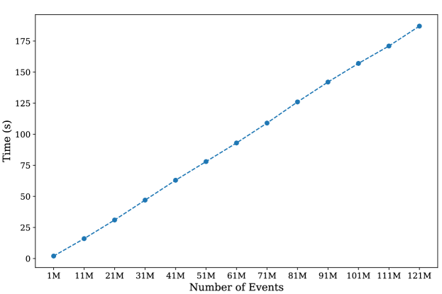
(a) raytracer

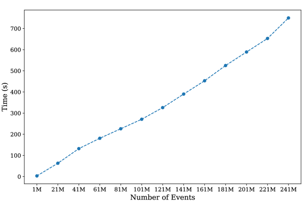
(b) sparsematmult

Figure 4. Scalability with number of events in the executions

Speedup over (Bertoni et al., 1989). Theoretical analysis indicates that our algorithm runs in $O(|\sigma|)$ time, while the algorithm in (Bertoni et al., 1989) runs in $O(|\sigma|^{\alpha})$ time. As shown in Table 2 and Table 3, our algorithm PatternTrack exhibits significant performance advantages over Bertoni in practice. Additionally, Bertoni is not scalable when the length of the execution increases, as evidenced by the numerous instances of “OOM” (Out of Memory) cases in the tables. This is because Bertoni needs to store all ideals of a partial order, which consumes $O(|\sigma|^{\alpha})$ space. As a result, this limits its scalability only to short executions. In contrast, our constant-space algorithm PatternTrack, catered to pattern regular languages, is not burdened by this limitation and can handle executions with millions of events.

Performance w.r.t. execution length. We next investigate whether the theoretical linear-time complexity of our algorithm also translates empirically. We selected two executions, from programs raytracer and sparsematmult, based on the fact that their length and the time taken to witness the first pattern match are both large. This selection criterion ensures that we can gather sufficient data to evaluate the performance across a range of execution lengths. To accomplish this, we recorded the time taken by our algorithm to process every 10 million events for raytracer and every 20 million events for sparsematmult. Figure 4 presents the result, and is in alignment with the theoretical linear running time of PatternTrack.

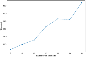
Figure 5. Performance over #threads

Performance w.r.t number of threads. The time taken by each vector clock operation is proportional to the number of threads, and we expect that PatternTrack’s running time is also proportional to this number. To test this assumption, we generated seven executions from benchmark raytracer with $5$, $10$, $15$, $20$, $25$, and $35$ threads respectively. The raytracer application allows us to configure the number of threads when generating executions. We then recorded the time taken by PatternTrack to process $1,000,000$ events for each execution. The results, in Figure 5, show that the time consumption increases as the number of threads increases, in line with PatternTrack’s theoretical complexity.

7. Related Work

Runtime verification has emerged as a popular class of techniques instrumental in popularizing the adoption of lightweight formal methods in large-scale industrial settings. Several classes of specifications such as LTL (Rosu and Havelund, 2005), extended regular expressions (Sen and Rosu, 2003), and CFG (Meredith et al., 2010) and techniques to monitor the runtime behaviour of the underlying software in conjunction with these specifications have been proposed. Aspect-oriented monitoring frameworks have been developed to bridge the gap between formal algorithms and practical tools. These include Java-MaC (Kim et al., 2004) and JavaMOP (Jin et al., 2012). However, such techniques are catered towards the problem of the “detection” of violations of these specifications at runtime, in contrast to the “prediction” problem, which we address in our work when the underlying software is concurrent or multi-threaded.

Predictive techniques have recently emerged as a fundamental paradigm to enhance the efficacy of runtime verification techniques — instead of focusing on bugs in the observed sequence of events, such techniques attempt to find bugs in alternate correct reorderings. Most works in the runtime predictive analysis are centered around the detection of implicit concurrency-centric specifications such as the presence of data races, deadlocks, or violations of atomicity. Some of the early works that studied predictive analysis for data races are instrumental in formulating core ideas such as sound and maximal causal models and correct reorderings (Sen et al., 2005, 2006; Chen and Rosu, 2007; Chen et al., 2008; Serbanuta et al., 2012; Said et al., 2011; Huang et al., 2015, 2014). Many of these techniques, however, primarily employ heavy-weight approaches such as exhaustive enumeration or the use of SAT/SMT solvers, limiting their scalability in practice. The focus of recent works in predictive analysis tools  (Cai et al., 2021; Kini et al., 2017; Mathur et al., 2021; Roemer and Bond, 2019; Roemer et al., 2020; Mathur et al., 2018; Pavlogiannis, 2019) has been on efficiency and practical scalability. Such techniques develop carefully crafted algorithms relying on specific heuristics or partial orders and avoid heavy-weight SMT solving. Beyond data races, recent improvements in these techniques have been used for predicting other concurrency bugs such as deadlocks (Cai et al., 2021; Sorrentino et al., 2010; Tunç et al., 2023; Kalhauge and Palsberg, 2018; Mathur et al., 2018). Some works also propose predictive methods for higher level, but specific properties such as use-after-free violations (Huang, 2018), null-pointer dereferences (Farzan et al., 2012), and violations of atomicity specifications (Farzan and Madhusudan, 2008, 2009; Flanagan et al., 2008a; Biswas et al., 2014; Sinha et al., 2011; Mathur and Viswanathan, 2020). Our work is a step towards adapting predictive techniques to explicitly defined specifications. GPredict (Huang et al., 2015) proposes the use of SMT solving for generalized predictive monitoring over explicitly defined specifications (under the maximal causality model) but has limited scalability.

We remark that for the case of implicitly defined bugs such as data races, the computational intractability (Mathur et al., 2020; Gibbons and Korach, 1997) in prediction arises primarily because of the exhaustive space of correct reorderings considered in these techniques (Smaragdakis et al., 2012; Serbanuta et al., 2012). Reasoning based on Mazurkiewicz traces, though less exhaustive, is in general more scalable. Indeed, the most widely adopted data race detection techniques crucially rely on the happens-before partial order (Poznianski and Schuster, 2003; Flanagan and Freund, 2009; Mathur et al., 2018) based on a Mazurkiewicz dependence relation, and typically run in linear time (assuming the alphabet is of constant size) or in low-degree polynomial time (when the alphabet is not constant (Kulkarni et al., 2021)). Our work has been inspired by this contrast in computational complexity of reasoning with Mazurkiewicz traces v/s correct reorderings. Unfortunately, though, our hardness result depicts that this insight does not trivially generalize to arbitrary properties beyond data races. Our work therefore proposes pattern languages to offer a good balance of expressiveness and algorithmic efficiency. Our central result essentially says that the trace closure of pattern languages is regular. A complete characterization of regular languages whose closure is regular is that of star-connected regular languages due to (Ochmański, 1985). However, this result does not immediately yield an algorithm to translate an arbitrary star-connected languages to an automaton that recognizes its trace closure. Languages generated by Alphabetic Pattern Constraints (APC) (Bouajjani et al., 2001) are a subclass of star-connected language, are closed under trace closure, and are strictly more expressive than generalized pattern languages. However, an efficient vector clock algorithm for predictive monitoring against APCs is not known. Our work thus fills the gap between theoretical results and practical techniques by designing small-sized monitors for predictive monitoring against pattern languages. The use of after sets in our constant space algorithm has been inspired from work in data race detection (Kini et al., 2018).

Soundness (absence of false positives), although highly desirable, often comes at a cost of computational complexity. Towards this, many runtime predictive analysis techniques often forego soundness in favour of the simplicity of analysis, including the Eraser algorithm based on locksets (Savage et al., 1997) or works on deadlock prediction (Cai et al., 2020; Bensalem and Havelund, 2005). Some approaches perform post-hoc analysis to reduce false positives (Roemer et al., 2018, 2020). Other approaches rely on re-executions to confirm the predicted bugs (Joshi et al., 2009; Sorrentino et al., 2010) to reduce false positives.

Concurrency bug detection has been an active area of research for several decades. Besides runtime verification and predictive monitoring, there are many other techniques for the analysis of concurrent programs. Model checking (Clarke et al., 1986) has emerged as a popular paradigm for finding bugs, thanks to advances such as dynamic partial order reduction (Flanagan and Godefroid, 2005) and stateless model checking (Abdulla et al., 2014; Kokologiannakis et al., 2019, 2022; Oberhauser et al., 2021). Randomized testing techniques (Joshi et al., 2009; Burckhardt et al., 2010; Ozkan et al., 2019; Yuan et al., 2018) as well as fuzz testing techniques (Jeong et al., 2019) have also been shown effective in practice. Static analysis techniques (Voung et al., 2007; Naik et al., 2006; Blackshear et al., 2018; Engler and Ashcraft, 2003) have been developed, but their adoption is often limited by high false positive rates. Type systems for preventing data races (Boyapati et al., 2002; Flanagan et al., 2008b; Flanagan and Qadeer, 2003) have been instrumental in the design of programming languages such as Rust.

8. Conclusions

In this work, we study the predictive monitoring problem — given an execution of a concurrent program, can it be reordered to witness the violation of a specification? We show that for specifications expressed using regular languages, and when the reorderings are restricted to the trace equivalence class of the observed execution, this problem suffers a high complexity polynomial lower bound. Towards this, we propose a sub-class of regular languages, called (generalized) pattern languages, and show that this class of languages can be effectively monitored, in a predictive sense, using a constant-space linear-time algorithm. Our experimental evaluation, using an implementation of the algorithm PatternTrack we develop, shows the effectiveness of our proposed class of specification languages and the algorithms for (predictive) monitoring against them.

There are many avenues for future work. We expect pattern languages to be useful in controlled concurrency testing techniques (Musuvathi and Qadeer, 2006; Agarwal et al., 2021) and fuzz testing for concurrent software (Jeong et al., 2019). Another interesting direction is to generalize the algorithms developed here to a larger class of temporal specifications, such as APCs (Bouajjani et al., 2001), which remain easier to write, are developer-friendly, and house the potential of widespread adoption. Building optimal stateless model checking (Kokologiannakis et al., 2022) algorithms for richer specifications such as pattern languages is another interesting direction.

Data Availability Statement

The artefact for this work is available (Ang and Mathur, 2023), which contains source code and benchmarks to reproduce our evaluation in Section 6.

Appendix A Proofs from Section 4

In this section, we prove the closure properties of pattern languages and generalized pattern languages (Theorem 4.4 and Theorem 4.5).

We first give proof of some closure properties of pattern languages $\mathtt{PATT}$.

Proof of Theorem 4.4.

We prove that the class of all pattern languages, $\mathtt{PATT}$, is closed under concatenation, but is not closed under union, intersection, complementation, and Kleene Star.

Pattern languages are not closed under union. We prove it by providing a counterexample. Let us consider two patterns $\texttt{Patt}_{a},\texttt{Patt}_{b}\in\mathtt{PATT}$, where $a\neq b\in\Sigma$. To prove by contradiction, we assume there is a pattern $\texttt{Patt}_{{c}_{1},\dots,{c}_{k}}\in\mathtt{PATT}$ such that $\texttt{Patt}_{{c}_{1},\dots,{c}_{k}}=\texttt{Patt}_{a}\cup\texttt{Patt}_{b}$. Since all the strings contained in $\texttt{Patt}_{{c}_{1},\dots,{c}_{k}}$ have a minimum length of $k$, and $a,b\in\texttt{Patt}_{{c}_{1},\dots,{c}_{k}}$, it implies that $k=1$. If $c_{1}\not\in\{a,b\}$, then $c_{1}$ belongs to $\texttt{Patt}_{c_{1}}$ but not to $\texttt{Patt}_{a}\cup\texttt{Patt}_{b}$. If $c_{1}=a$, then $b$ belongs to $\texttt{Patt}_{b}$ but not to $\texttt{Patt}_{c_{1}}$. Similarly, $c_{1}=b$ also leads to a contradiction. From the above cases, we can conclude that no pattern equals the union of $\texttt{Patt}_{a}$ and $\texttt{Patt}_{b}$.

Pattern languages are not closed under intersection. A counterexample, in this case, is that $\texttt{Patt}_{a}\cap\texttt{Patt}_{b}$ cannot be written as a pattern language. We assume that, by contradiction, there is a pattern $\texttt{Patt}_{{c}_{1},\dots,{c}_{k}}\in\mathtt{PATT}$ such that $\texttt{Patt}_{{c}_{1},\dots,{c}_{k}}=\texttt{Patt}_{a}\cap\texttt{Patt}_{b}$. Since $ab$ and $ba$ belong to $\texttt{Patt}_{a}\cap\texttt{Patt}_{b}$, $k$ is at most 2.

If $k=1$, $c_{1}\in\texttt{Patt}_{c_{1}}=\texttt{Patt}_{a}\cap\texttt{Patt}_{b}$. But $c_{1}$ cannot be $a$ and $b$ at the same time. Then $k=2$. Observe that $ab,ba\in\texttt{Patt}_{c_{1},c_{2}}$. However, $c_{1},c_{2}$ do not exist because they should be $ab$ and $ba$ at the same time. From the above contradictions, we conclude that $\texttt{Patt}_{a}\cap\texttt{Patt}_{b}$ is not a pattern language. Thus pattern languages are not closed under intersection.

Pattern languages are not closed under complementation. Here is a counterexample. Consider the pattern language $L=\texttt{Patt}_{a}$. $L^{c}=(\Sigma\setminus\{a\})^{*}$, which contains all the strings without the occurrence of $a$. By contradiction, we assume that there is a $\texttt{Patt}_{{b}_{1},\dots,{b}_{k}}\in\mathtt{PATT}$ such that $\texttt{Patt}_{{b}_{1},\dots,{b}_{k}}=L^{c}$. However, observe that $a\cdot b_{1}\cdot\dots\cdot b_{k}\in\texttt{Patt}_{{b}_{1},\dots,{b}_{k}}$, which gives us a contradiction.

Pattern languages are closed under concatenation. For any two pattern languages $L_{1}=\texttt{Patt}_{{a}_{1},\dots,{a}_{d}}$ and $L_{2}=\texttt{Patt}_{{b}_{1},\dots,{b}_{l}}$, we claim that the language $L=\texttt{Patt}_{{a}_{1},\dots,{a}_{d}\circ{b}_{1},\dots,{b}_{l}}$ is indeed the concatenation of $L_{1}$ and $L_{2}$, i.e., $L=L_{1}\circ L_{2}$.

Pattern languages are not closed under Kleene star. We first observe that the only pattern language that contains $\varepsilon$ is $\Sigma^{*}$, which is a pattern language when $d=0$. $\varepsilon\in(\texttt{Patt}_{a,a})^{*}$ implies that $(\texttt{Patt}_{a,a})^{*}=\Sigma^{*}$. However, $a\in\Sigma^{*}$ does not belong to $(\texttt{Patt}_{a,a})^{*}$, which contains either an empty string or a string with at least two $a$s. Thus, $(\texttt{Patt}_{a,a})^{*}$ is not a generalized pattern language, which gives a counterexample.

∎

In the following, we prove some closure properties of generalized pattern languages.

Proof of Theorem 4.5.

We prove that the class of all generalized pattern languages is closed under union, intersection, concatenation, and Kleene Star, but is not closed under complementation.

Generalized pattern languages are closed under union. Consider two generalized pattern languages $L_{1}=\bigcup_{i\in I}L_{1,i}$ and $L_{2}=\bigcup_{j\in J}L_{2,j}$, where each of $\{L_{1,i},L_{2,j}\}_{i\in I,j\in J}$ is one of the following: pattern language, $\{\varepsilon\}$, or $\varnothing$. From the definition, we know that $L_{1}\cup L_{2}=(\bigcup_{i\in I}L_{1,i})\bigcup(\bigcup_{j\in J}L_{2,j})$ is a generalized pattern language.

Generalized pattern languages are closed under intersection. We first consider the intersection of two pattern languages. We have proved that pattern languages are not closed under intersection, but we claim that the intersection of two pattern languages is a generalized pattern language. For any two pattern languages $L_{1}=\texttt{Patt}_{{a}_{1},\dots,{a}_{k}}$ and $L_{2}=\texttt{Patt}_{{b}_{1},\dots,{b}_{l}}$, $L_{1}\cap L_{2}=\bigcup_{w\in W}\texttt{Patt}_{w}$, where

$$W={a}_{1},\dots,{a}_{d}\odot{b}_{1},\dots,{b}_{l}$$

Notice that $|W|$ is bounded because the length of $w\in W$ is bounded by $k+l$. Now we prove equality.

1. ($L_{1}\cap L_{2}\subseteq\bigcup_{w\in W}\texttt{Patt}_{w}$) For any $\sigma\in L_{1}\cap L_{2}$, there must be two subsequences $w_{1}$ and $w_{2}$ of $\sigma$ such that $w_{1}={a}_{1},\dots,{a}_{k}$ and $w_{2}={b}_{1},\dots,{b}_{l}$. Consider the smallest subsequence $w^{\prime}$ of $\sigma$ such that $w_{1}$ and $w_{2}$ are subsequences of $w^{\prime}$. Clearly, $w^{\prime}\in W$, which implies that $\sigma\in\bigcup_{w\in W}\texttt{Patt}_{w}$.

2. ($\bigcup_{w\in W}\texttt{Patt}_{w}\subseteq L_{1}\cap L_{2}$) For any $\sigma\in\bigcup_{w\in W}\texttt{Patt}_{w}$, there exists a $w\in W$ such that $\sigma\in\texttt{Patt}_{w}$. Since ${a}_{1},\dots,{a}_{k}$ and ${b}_{1},\dots,{b}_{l}$ are both subsequences of $w$, they are also subsequences of $\sigma$, which directly gives us $\sigma\in L_{1}\cap L_{2}$.

Now we turn our focus on the original closure property of generalized pattern languages. Consider two generalized pattern languages $L_{1}=\bigcup_{i\in I}L_{1,i}$ and $L_{2}=\bigcup_{j\in J}L_{2,j}$, where each of $\{L_{1,i},L_{2,j}\}_{i\in I,j\in J}$ is one of the following: pattern language, $\{\varepsilon\}$, or $\varnothing$. Their intersection is $L_{1}\cap L_{2}=\bigcup_{i\in I,j\in J}L_{1,i}\cap L_{2,j}$. Now consider the following cases:

1. $L_{1,i}$ and $L_{2,j}$ are both pattern languages. From above, $L_{1,i}\cap L_{2,j}$ is a union of pattern languages.

2. $L_{1,i}=\{\varepsilon\}$ and $L_{2,j}=\{\varepsilon\}$. Then $L_{1,i}\cap L_{2,j}=\{\varepsilon\}$.

3. One of $L_{1,i},L_{2,j}$ is $\{\varepsilon\}$ and the other is not. Then $L_{1,i}\cap L_{2,j}=\varnothing$.

4. At least one of $L_{1,i},L_{2,j}$ is $\varnothing$. Then $L_{1,i}\cap L_{2,j}=\varnothing$.

We can conclude from the above cases that $L_{1,i}\cap L_{2,j}$ is one of the following: a union of pattern languages, $\{\varepsilon\}$, or $\varnothing$. Hence, $L_{1}\cap L_{2}$ is a generalized pattern language.

Generalized pattern languages are not closed under complementation. We present a similar counterexample here. Consider the pattern language $L=\texttt{Patt}_{a}$. $L^{c}=(\Sigma\setminus\{a\})^{*}$, which contains all the strings without the occurrence of $a$. By contradiction, we assume that there is a generalized pattern language $L^{\prime}=\bigcup_{i\in I}L_{i}$ where $L_{i}$ is one of the following: pattern language, $\{\varepsilon\}$, or $\varnothing$. If no $L_{i}$ is a pattern language, then $L^{\prime}=\{\varepsilon\}$, which cannot be $\bigcup_{i\in I}L_{i}$. Then, without loss of generality, $L_{1}$ is a pattern language and is $\texttt{Patt}_{{b}_{1},\dots,{b}_{l}}$. $a\cdot b_{1}\cdot\dots\cdot b_{k}$ belongs to $\texttt{Patt}_{{b}_{1},\dots,{b}_{k}}$, thus belongs to $L^{\prime}$, which gives a contradiction because, by assumption, $L^{\prime}=L^{c}=(\Sigma\setminus\{a\})$.

Generalized pattern languages are closed under concatenation. Consider two generalized pattern languages $L_{1}=\bigcup_{i\in I}L_{1,i}$ and $L_{2}=\bigcup_{j\in J}L_{2,j}$, where each of $\{L_{1,i},L_{2,j}\}_{i\in I,j\in J}$ is one of the following: pattern language, $\{\varepsilon\}$, or $\varnothing$. Their concatenation is $L_{1}\circ L_{2}=\bigcup_{i\in I,j\in J}L_{1,i}\circ L_{2,j}$. Now consider the following cases:

1. $L_{1,i}$ and $L_{2,j}$ are both pattern languages. $L_{1,i}\circ L_{2,j}$ is also a pattern language because pattern languages are closed under concatenation.

2. $L_{1,i}=\{\varepsilon\}$ or $L_{2,j}=\{\varepsilon\}$. We consider, without loss of generality, the first case that $L_{1,i}=\{\varepsilon\}$. Then $L_{1,i}\circ L_{2,j}=L_{2,j}$.

3. $L_{1,i}=\varnothing$ or $L_{2,j}=\varnothing$. For either case, we have $L_{1,i}\circ L_{2,j}=\varnothing$.

We can conclude from the above cases that $L_{1,i}\circ L_{2,j}$ is still one of the following: pattern language, $\{\varepsilon\}$, or $\varnothing$. Hence, $L_{1}\circ L_{2}$ is a generalized pattern language.

Generalized pattern languages are closed under Kleene star. We claim $L^{*}=L\cup\{\varepsilon\}$, where $L$ is a generalized pattern language. One direction that $L\cup\{\varepsilon\}\subseteq L^{*}$ is trivial. Now consider $L^{*}\subseteq L\cup\{\varepsilon\}$, which will be proved by induction that for all $n>0$, $L^{n}\subseteq L\cup\{\varepsilon\}$.

1. (Base case) $L^{0}=\{\varepsilon\}\subseteq L\cup\{\varepsilon\}$.

2. (Inductive case) Assume that $L^{k}\subseteq L\cup\{\varepsilon\}$. $L^{k+1}=L^{k}\circ L$. Consider $\sigma\in L^{k+1}=L^{k}\circ L$. We can break down $\sigma$ into two parts $\sigma=\sigma_{1}\circ\sigma_{2}$, such that $\sigma_{1}\in L^{k}\subseteq L\cup\{\varepsilon\}$ and $\sigma_{2}\in L$. From the definition of generalized pattern language, $\sigma_{1}$ must be either $\varepsilon$ or a member of the pattern language $\texttt{Patt}_{{a}_{1},\dots,{a}_{d}}\subseteq L$. If $\sigma_{1}=\varepsilon$, then $\sigma=\sigma_{2}\in L\subseteq L\cup\{\varepsilon\}$. In the other case that $\sigma_{1}\in\texttt{Patt}_{{a}_{1},\dots,{a}_{d}}$, observe that $\sigma=\sigma_{1}\circ\sigma_{2}$ is also a member of $\texttt{Patt}_{{a}_{1},\dots,{a}_{d}}$, because $\sigma_{2}\in\Sigma^{*}$ which is the last composition of $\texttt{Patt}_{{a}_{1},\dots,{a}_{d}}$. Thus, $\sigma\in L\subseteq L\cup\{\varepsilon\}$.

Notice that $L\cup\{\varepsilon\}$ is also a generalized pattern language, implying that generalized Pattern Languages are closed under the Kleene star.

∎

Appendix B Proofs from Section 5

B.1. Proofs from Section 5.2

Proof of Lemma 5.3.

Let $\tau^{\dagger}=\mathsf{sort}({\tau},{\langle a_{j_{1}},\dots,a_{j_{m}}\rangle})=\langle e_{i^{\dagger}_{1}},\dots,e_{i^{\dagger}_{m}}\rangle$. What we need to prove is that

$$\exists\sigma^{\prime}\equiv_{\mathcal{I}}\sigma,\tau^{\dagger}\text{ is a subsequence of }\sigma^{\prime}\iff\forall i^{\dagger}_{r}\neq i^{\dagger}_{s},s<r\Rightarrow e_{i^{\dagger}_{r}}\not\leq^{\sigma}_{\mathcal{D}}e_{i^{\dagger}_{s}}$$

($\Rightarrow$) We assume that, by contradiction, there are $r,s$ such that $s<r$ and $e_{i^{\dagger}_{r}}\leq^{\sigma}_{\mathcal{D}}e_{i^{\dagger}_{s}}$. However, the latter assumption contradicts the fact that $e_{i^{\dagger}_{r}}$ occurs after $e_{i^{\dagger}_{s}}$ in $\sigma^{\prime}$ and $\sigma^{\prime}$ follows the same partial order as $\sigma$.

($\Leftarrow$) Consider the underlying directed acyclic graph $G_{\sigma}$ of the partial order $\leq^{\sigma}_{\mathcal{D}}$ induced by $\sigma$. The left-hand side is equivalent to say, adding edges $(e_{i^{\dagger}_{j}},e_{i^{\dagger}_{j+1}})$, $1\leq j\leq m-1$, to $G_{\sigma}$ does not change its acyclicity. Then a linearization of the new graph is equivalent to $\sigma$, and also, has a subsequence $\tau^{\dagger}$.

Let us prove this by contradiction. Assume that the new graph $G_{\sigma\cup\tau^{\dagger}}$ is not acyclic. Then We prove that there must be a bad cycle that consists of edges from $\{(e_{i^{\dagger}_{j}},e_{i^{\dagger}_{j+1}})\,|\,1\leq j\leq m-1\}$, which is a contradiction since those edges form a chain. We do induction on the number of edges in the cycle that come from $G_{\sigma}$. The base case when the number is zero is trivial. We assume that if there is a cycle containing less than or equal to $k$ edges coming from $G_{\sigma}$, then there is a bad cycle in the graph. Consider a cycle that contains $k+1$ coming from $G_{\sigma}$. There must be two different nodes $e_{i^{\dagger}_{r}}$ and $e_{i^{\dagger}_{s}}$ linked by a chain of edges from $G_{\sigma}$. Otherwise, the whole cycle consists of edges from $G_{\sigma}$, which is acyclic. Then $e_{i^{\dagger}_{r}}\leq^{\sigma}_{\mathcal{D}}e_{i^{\dagger}_{s}}$, which implies $r<s$. Thus, there is a chain of edges $(e_{i^{\dagger}_{r}},e_{i^{\dagger}_{r+1}}),\dots,(e_{i^{\dagger}_{s-1}},e_{i^{\dagger}_{s}})$ from $e_{i^{\dagger}_{r}}$ to $e_{i^{\dagger}_{s}}$. Now we get a cycle containing less than or equal to $k$ edges coming from $G_{\sigma}$, which implies the existence of a bad cycle. Consequently, if the new graph is not acyclic, there must be a bad cycle that cannot exist. ∎

Now we prove the correctness of incremental updates of after sets.

Proof of Lemma 5.6.

From the definition, $\mathsf{After}_{\rho\circ f}(e)$ is defined as

$$\mathsf{After}_{\rho\circ f}(e)=\begin{cases}\mathsf{After}_{\rho}(e)\cup\{\mathsf{lab}(f)\}&\text{ if }e\leq^{\rho\circ f}_{\mathcal{D}}f,\\ \mathsf{After}_{\rho}(e)&\text{ otherwise}.\end{cases}$$

We will prove that $e\leq^{\rho\circ f}_{\mathcal{D}}f$ iff there exists $a\in\mathsf{After}_{\rho}(e)$ such that $(a,\mathsf{lab}(f))\not\in\mathcal{I}$.

($\Leftarrow$) Assume that $a\in\mathsf{After}_{\rho}(e)$ such that $(a,\mathsf{lab}(f))\not\in\mathcal{I}$. Since $a\in\mathsf{After}_{\rho}(e)$, from the definition, there is an event $e^{\prime}\in\rho$ such that $e\leq^{\rho}_{\mathcal{D}}e^{\prime}$ and $\mathsf{lab}(e^{\prime})=a$. Moreover, we have $e^{\prime}\leq^{\rho}_{\mathcal{D}}f$ because $(a,\mathsf{lab}(f))\not\in\mathcal{I}$. By transitivity, $e\leq^{\rho\circ f}_{\mathcal{D}}f$.

($\Rightarrow$) From the definition of the partial order $\leq^{\rho\circ f}_{\mathcal{D}}$, $e\leq^{\rho\circ f}_{\mathcal{D}}f$ implies that there is an event $e^{\prime}\in\rho$ such that $e\leq^{\rho}_{\mathcal{D}}e^{\prime}$ and $(\mathsf{lab}(e^{\prime}),\mathsf{lab}(f))\not\in\mathcal{I}$. So $\mathsf{lab}(e^{\prime})\in\mathsf{After}_{\rho}(e)$ by definition of after set, which provides an instance of $a$ on the right-hand side.

∎

B.2. Proofs from Section 5.3

Before we prove the existence of the maximum element in a complete set of partially admissible tuples, we prove that the set is closed under the join operation.

Proof of Lemma 5.8.

Let $\tau_{1}=\langle{e^{1}}_{1},\dots,{e^{1}}_{m}\rangle,\tau_{2}=\langle{e^{2}}_{1},\dots,{e^{2}}_{m}\rangle$, such that $\mathsf{lab}(\tau_{1})=\mathsf{lab}(\tau_{2})=\langle{b}_{1},\dots,{b}_{m}\rangle$. Let $\tau_{1}\bigtriangledown\tau_{2}=\langle{e}_{1},\dots,{e}_{m}\rangle$, where for $1\leq i\leq m$, $e_{i}=e^{2}_{i}$ if $e^{1}_{i}<^{\sigma}e^{2}_{i}$, or $e^{1}_{i}$ otherwise. It is obvious that $\mathsf{lab}(\tau_{1}\bigtriangledown\tau_{2})=\langle{b}_{1},\dots,{b}_{m}\rangle$. We will prove that $\tau_{1}\bigtriangledown\tau_{2}$ is a partially locally admissible tuple.

Let $\langle a_{j_{1}},\dots,a_{j_{m}}\rangle$ be a subsequence of $a_{1},\dots,a_{d}$ and a permutation of $\langle{b}_{1},\dots,{b}_{m}\rangle$. Notice that the reordering of $\mathsf{sort}$ only depends on the labels. Therefore, let

$$\langle e^{1}_{i^{\dagger}_{1}},\dots,e^{1}_{i^{\dagger}_{m}}\rangle=\mathsf{sort}({\tau_{1}},{\langle a_{j_{1}},\dots,a_{j_{m}}\rangle}),$$

$$\langle e^{2}_{i^{\dagger}_{1}},\dots,e^{2}_{i^{\dagger}_{m}}\rangle=\mathsf{sort}({\tau_{2}},{\langle a_{j_{1}},\dots,a_{j_{m}}\rangle}),$$

$$\langle e_{i^{\dagger}_{1}},\dots,e_{i^{\dagger}_{m}}\rangle=\mathsf{sort}({\tau_{1}\bigtriangledown\tau_{2}},{\langle a_{j_{1}},\dots,a_{j_{m}}\rangle}).$$

Since $\tau_{1}$ and $\tau_{2}$ are admissible, for all $i^{\dagger}_{r}\neq i^{\dagger}_{s}$, we have $s<r\Rightarrow e^{1}_{i^{\dagger}_{r}}\not\leq^{\sigma}_{\mathcal{D}}e^{1}_{i^{\dagger}_{s}}$ and $e^{2}_{i^{\dagger}_{r}}\not\leq^{\sigma}_{\mathcal{D}}e^{2}_{i^{\dagger}_{s}}$.

For any $i^{\dagger}_{r}\neq i^{\dagger}_{s}$ such that $s<r$, we prove that $e_{i^{\dagger}_{r}}\not\leq^{\sigma}_{\mathcal{D}}e_{i^{\dagger}_{s}}$ by contradiction. Assume that $e_{i^{\dagger}_{r}}\leq^{\sigma}_{\mathcal{D}}e_{i^{\dagger}_{s}}$. It is impossible that both $e_{i^{\dagger}_{r}}$ and $e_{i^{\dagger}_{s}}$ come from the same source, $\tau_{1}$ or $\tau_{2}$. Without loss of generality, let $e_{i^{\dagger}_{r}}=e^{1}_{i^{\dagger}_{r}}$ and $e_{i^{\dagger}_{s}}=e^{2}_{i^{\dagger}_{s}}$. Then we have $e^{2}_{i^{\dagger}_{r}}<^{\sigma}e^{1}_{i^{\dagger}_{r}}\leq^{\sigma}_{\mathcal{D}}e^{2}_{i^{\dagger}_{s}}$, which contradicts to the fact that $\tau_{2}$ is locally admissible. This concludes that $\tau_{1}\bigtriangledown\tau_{2}$ is admissible. ∎

Now let us prove the existence of the maximum element.

Proof of Lemma 5.7.

In short, the set ${\partial}\mathsf{AdTpls}({\rho},{\langle{b}_{1},\dots,{b}_{m}\rangle})$ and the join operations give a join-semilattice, resulting in the existence of the maximum element. Also, it is easy to check that the unique maximum element is exactly $\bigtriangledown_{\tau\in{\partial}\mathsf{AdTpls}({\rho},{\langle{b}_{1},\dots,{b}_{m}\rangle})}\tau$. ∎

Let us prove Lemma 5.9 demonstrating the way we keep track of the maximum element of ${\partial}\mathsf{AdTpls}({\rho},{\langle{b}_{1},\dots,{b}_{m}\rangle})$ along the prefix $\rho$.

Proof of Lemma 5.9.

If $\mathsf{lab}(f)=b_{m}$ and $\max({\partial}\mathsf{AdTpls}({\rho},{\langle{b}_{1},\dots,{b}_{m-1}\rangle}))\circ f$ is partially admissible, then it is obvious that

$$\max({\partial}\mathsf{AdTpls}({\rho\circ f},{\langle{b}_{1},\dots,{b}_{m}\rangle}))=\max({\partial}\mathsf{AdTpls}({\rho},{\langle{b}_{1},\dots,{b}_{m-1}\rangle}))\circ f,$$

since for all $\langle{e}_{1},\dots,{e}_{m}\rangle\in{\partial}\mathsf{AdTpls}({\rho\circ f},{\langle{b}_{1},\dots,{b}_{m}\rangle})$, we have

$$\langle{e}_{1},\dots,{e}_{m-1}\rangle\unlhd\max({\partial}\mathsf{AdTpls}({\rho},{\langle{b}_{1},\dots,{b}_{m-1}\rangle}))\text{ and }e_{m}<^{\rho\circ f}f.$$

If $\mathsf{lab}(f)\neq b_{m}$, then the set of admissible tuples of label $\langle{b}_{1},\dots,{b}_{m}\rangle$ is unchanged from $\rho$ to $\rho\circ f$. The remaining is to prove that when $\mathsf{lab}(f)=b_{m}$ and $\max({\partial}\mathsf{AdTpls}({\rho},{\langle{b}_{1},\dots,{b}_{m-1}\rangle}))\circ f$ is not partially admissible, $\max({\partial}\mathsf{AdTpls}({\rho\circ f},{\langle{b}_{1},\dots,{b}_{m}\rangle}))=\max({\partial}\mathsf{AdTpls}({\rho},{\langle{b}_{1},\dots,{b}_{m}\rangle}))$.

By contraction, assume $\max({\partial}\mathsf{AdTpls}({\rho\circ f},{\langle{b}_{1},\dots,{b}_{m}\rangle}))\neq\max({\partial}\mathsf{AdTpls}({\rho},{\langle{b}_{1},\dots,{b}_{m}\rangle}))$. Then $\max({\partial}\mathsf{AdTpls}({\rho\circ f},{\langle{b}_{1},\dots,{b}_{m}\rangle}))$ must be a tuple ending with $f$.

Let $\max({\partial}\mathsf{AdTpls}({\rho\circ f},{\langle{b}_{1},\dots,{b}_{m}\rangle}))=\langle{e}_{1},\dots,{e}_{m-1},f\rangle$, where we also have $\langle{e}_{1},\dots,{e}_{m-1}\rangle\in{\partial}\mathsf{AdTpls}({\rho},{\langle{b}_{1},\dots,{b}_{m-1}\rangle})$. Let $\max({\partial}\mathsf{AdTpls}({\rho},{\langle{b}_{1},\dots,{b}_{m-1}\rangle}))=\langle{e^{\prime}}_{1},\dots,{e^{\prime}}_{m-1}\rangle$. Then for all $1\leq i\leq m-1$, $e_{i}<^{\rho}e^{\prime}_{i}$.

Since $\max({\partial}\mathsf{AdTpls}({\rho},{\langle{b}_{1},\dots,{b}_{m-1}\rangle}))\circ f$ is not partially admissible, there must be a $e^{\prime}_{i}$ which should occur after $f$ in pattern $\langle{a}_{1},\dots,{a}_{m}\rangle$ but is partially ordered with $f$, $e^{\prime}_{i}\leq^{\rho\circ f}_{\mathcal{D}}f$. Then we have $e_{i}<^{\rho}e^{\prime}_{i}\leq^{\rho\circ f}_{\mathcal{D}}f$, which contradicts with the fact that $\langle{e}_{1},\dots,{e}_{m-1},f\rangle$ is admissible. Hence, we have $\max({\partial}\mathsf{AdTpls}({\rho\circ f},{\langle{b}_{1},\dots,{b}_{m}\rangle}))=\max({\partial}\mathsf{AdTpls}({\rho},{\langle{b}_{1},\dots,{b}_{m}\rangle}))$.

∎

B.3. Proofs from Section 5.4

Finally, we present the proof of the correctness of Algorithm 3.

Proof of Theorem 5.10.

The correctness of the algorithm can be shown by a loop invariant:

For the prefix $\rho\circ f$ of $\sigma$ and for any permutation of prefixes of ${a}_{1},\dots,{a}_{d}$, $\langle{b}_{1},\dots,{b}_{m}\rangle$.

$$M(\langle{b}_{1},\dots,{b}_{m}\rangle)=\langle\mathsf{After}_{\rho\circ f}(e_{1}),\dots,\mathsf{After}_{\rho\circ f}(e_{m})\rangle,$$

where $\langle{e}_{1},\dots,{e}_{m}\rangle=\max({\partial}\mathsf{AdTpls}({\rho\circ f},{\langle{b}_{1},\dots,{b}_{m}\rangle}))$.

The loop in the algorithm keeps track of the maximum element of each set in the form of after sets. The correctness of the loop invariant follows $Lemma~{}\ref{lem:aft-incre}$ and $Lemma~{}\ref{lem:comp-max}$.

Finally, the predictive monitoring problem answers “YES” if and only if there is an admissible tuple of length $k$. This is equivalent to the existence of the maximum element of length $k$ after processing some prefix of $\sigma$, which is also equivalent to the case that our algorithm returns “YES”.

∎

References

- (1)
- ant (2023) 2023. AntLRWorks. https://github.com/antlr/antlrworks. [Online; accessed 24-October-2023].
- exp (2023) 2023. exp4j. https://github.com/fasseg/exp4j. [Online; accessed 24-October-2023].
- jfr (2023) 2023. JFreeChart. https://github.com/jfree/jfreechart. [Online; accessed 24-October-2023].
- log (2023) 2023. Logstash Logback Encoder. https://github.com/logfellow/logstash-logback-encoder. [Online; accessed 24-October-2023].
- zer (2023) 2023. ZeroMQ log4j appender. https://github.com/lusis/zmq-appender. [Online; accessed 24-October-2023].
- Abdulla et al. (2014) Parosh Aziz Abdulla, Stavros Aronis, Bengt Jonsson, and Konstantinos Sagonas. 2014. Optimal dynamic partial order reduction. In The 41st Annual ACM SIGPLAN-SIGACT Symposium on Principles of Programming Languages, POPL ’14, San Diego, CA, USA, January 20-21, 2014, Suresh Jagannathan and Peter Sewell (Eds.). ACM, 373–384. https://doi.org/10.1145/2535838.2535845
- Abdulla et al. (2019) Parosh Aziz Abdulla, Jatin Arora, Mohamed Faouzi Atig, and Shankaranarayanan Krishna. 2019. Verification of Programs under the Release-Acquire Semantics. In Proceedings of the 40th ACM SIGPLAN Conference on Programming Language Design and Implementation (Phoenix, AZ, USA) (PLDI 2019). Association for Computing Machinery, New York, NY, USA, 1117–1132. https://doi.org/10.1145/3314221.3314649
- Agarwal et al. (2021) Udit Agarwal, Pantazis Deligiannis, Cheng Huang, Kumseok Jung, Akash Lal, Immad Naseer, Matthew Parkinson, Arun Thangamani, Jyothi Vedurada, and Yunpeng Xiao. 2021. Nekara: Generalised Concurrency Testing. In 2021 36th IEEE/ACM International Conference on Automated Software Engineering (ASE). 679–691. https://doi.org/10.1109/ASE51524.2021.9678838
- Agrawal and Srikant (1995) Rakesh Agrawal and Ramakrishnan Srikant. 1995. Mining Sequential Patterns. In Proceedings of the Eleventh International Conference on Data Engineering, March 6-10, 1995, Taipei, Taiwan, Philip S. Yu and Arbee L. P. Chen (Eds.). IEEE Computer Society, 3–14. https://doi.org/10.1109/ICDE.1995.380415
- Alur et al. (2004) Rajeev Alur, Kousha Etessami, and P. Madhusudan. 2004. A Temporal Logic of Nested Calls and Returns. In Tools and Algorithms for the Construction and Analysis of Systems, 10th International Conference, TACAS 2004, Held as Part of the Joint European Conferences on Theory and Practice of Software, ETAPS 2004, Barcelona, Spain, March 29 - April 2, 2004, Proceedings (Lecture Notes in Computer Science, Vol. 2988), Kurt Jensen and Andreas Podelski (Eds.). Springer, 467–481. https://doi.org/10.1007/978-3-540-24730-2_35
- Ang and Mathur (2023) Zhendong Ang and Umang Mathur. 2023. Predictive Monitoring against Pattern Regular Languages. https://doi.org/10.5281/zenodo.8424626 Artifact.
- Artho et al. (2003) Cyrille Artho, Klaus Havelund, and Armin Biere. 2003. High-level data races. Softw. Test. Verification Reliab. 13, 4 (2003), 207–227. https://doi.org/10.1002/STVR.281
- Bensalem and Havelund (2005) Saddek Bensalem and Klaus Havelund. 2005. Dynamic Deadlock Analysis of Multi-threaded Programs. In Hardware and Software Verification and Testing, First International Haifa Verification Conference, Haifa, Israel, November 13-16, 2005, Revised Selected Papers (Lecture Notes in Computer Science, Vol. 3875), Shmuel Ur, Eyal Bin, and Yaron Wolfsthal (Eds.). Springer, 208–223. https://doi.org/10.1007/11678779_15
- Bertoni et al. (1989) A. Bertoni, G. Mauri, and N. Sabadini. 1989. Membership problems for regular and context-free trace languages. Information and Computation 82, 2 (1989), 135–150. https://doi.org/10.1016/0890-5401(89)90051-5
- Biswas et al. (2014) Swarnendu Biswas, Jipeng Huang, Aritra Sengupta, and Michael D. Bond. 2014. DoubleChecker: efficient sound and precise atomicity checking. In ACM SIGPLAN Conference on Programming Language Design and Implementation, PLDI ’14, Edinburgh, United Kingdom - June 09 - 11, 2014, Michael F. P. O’Boyle and Keshav Pingali (Eds.). ACM, 28–39. https://doi.org/10.1145/2594291.2594323
- Blackburn et al. (2006) Stephen M. Blackburn, Robin Garner, Chris Hoffmann, Asjad M. Khan, Kathryn S. McKinley, Rotem Bentzur, Amer Diwan, Daniel Feinberg, Daniel Frampton, Samuel Z. Guyer, Martin Hirzel, Antony L. Hosking, Maria Jump, Han Bok Lee, J. Eliot B. Moss, Aashish Phansalkar, Darko Stefanovic, Thomas VanDrunen, Daniel von Dincklage, and Ben Wiedermann. 2006. The DaCapo benchmarks: java benchmarking development and analysis. In Proceedings of the 21th Annual ACM SIGPLAN Conference on Object-Oriented Programming, Systems, Languages, and Applications, OOPSLA 2006, October 22-26, 2006, Portland, Oregon, USA, Peri L. Tarr and William R. Cook (Eds.). ACM, 169–190. https://doi.org/10.1145/1167473.1167488
- Blackshear et al. (2018) Sam Blackshear, Nikos Gorogiannis, Peter W. O’Hearn, and Ilya Sergey. 2018. RacerD: Compositional Static Race Detection. Proc. ACM Program. Lang. 2, OOPSLA, Article 144 (oct 2018), 28 pages. https://doi.org/10.1145/3276514
- Bouajjani et al. (2001) Ahmed Bouajjani, Anca Muscholl, and Tayssir Touili. 2001. Permutation Rewriting and Algorithmic Verification. In 16th Annual IEEE Symposium on Logic in Computer Science, Boston, Massachusetts, USA, June 16-19, 2001, Proceedings. IEEE Computer Society, 399–408. https://doi.org/10.1109/LICS.2001.932515
- Boyapati et al. (2002) Chandrasekhar Boyapati, Robert Lee, and Martin C. Rinard. 2002. Ownership types for safe programming: preventing data races and deadlocks. In Proceedings of the 2002 ACM SIGPLAN Conference on Object-Oriented Programming Systems, Languages and Applications, OOPSLA 2002, Seattle, Washington, USA, November 4-8, 2002, Mamdouh Ibrahim and Satoshi Matsuoka (Eds.). ACM, 211–230. https://doi.org/10.1145/582419.582440
- Burckhardt et al. (2010) Sebastian Burckhardt, Pravesh Kothari, Madanlal Musuvathi, and Santosh Nagarakatte. 2010. A Randomized Scheduler with Probabilistic Guarantees of Finding Bugs. In Proceedings of the Fifteenth International Conference on Architectural Support for Programming Languages and Operating Systems (Pittsburgh, Pennsylvania, USA) (ASPLOS XV). Association for Computing Machinery, New York, NY, USA, 167–178. https://doi.org/10.1145/1736020.1736040
- Cai et al. (2020) Yan Cai, Ruijie Meng, and Jens Palsberg. 2020. Low-overhead deadlock prediction. In ICSE ’20: 42nd International Conference on Software Engineering, Seoul, South Korea, 27 June - 19 July, 2020, Gregg Rothermel and Doo-Hwan Bae (Eds.). ACM, 1298–1309. https://doi.org/10.1145/3377811.3380367
- Cai et al. (2021) Yan Cai, Hao Yun, Jinqiu Wang, Lei Qiao, and Jens Palsberg. 2021. Sound and efficient concurrency bug prediction. In ESEC/FSE ’21: 29th ACM Joint European Software Engineering Conference and Symposium on the Foundations of Software Engineering, Athens, Greece, August 23-28, 2021, Diomidis Spinellis, Georgios Gousios, Marsha Chechik, and Massimiliano Di Penta (Eds.). ACM, 255–267. https://doi.org/10.1145/3468264.3468549
- Calabro et al. (2009) Chris Calabro, Russell Impagliazzo, and Ramamohan Paturi. 2009. The Complexity of Satisfiability of Small Depth Circuits. In Parameterized and Exact Computation: 4th International Workshop, IWPEC 2009, Copenhagen, Denmark, September 10-11, 2009, Revised Selected Papers. Springer-Verlag, Berlin, Heidelberg, 75–85. https://doi.org/10.1007/978-3-642-11269-0_6
- Chen and Rosu (2007) Feng Chen and Grigore Rosu. 2007. Parametric and Sliced Causality. In Computer Aided Verification, 19th International Conference, CAV 2007, Berlin, Germany, July 3-7, 2007, Proceedings (Lecture Notes in Computer Science, Vol. 4590), Werner Damm and Holger Hermanns (Eds.). Springer, 240–253. https://doi.org/10.1007/978-3-540-73368-3_27
- Chen et al. (2008) Feng Chen, Traian-Florin Serbanuta, and Grigore Rosu. 2008. jPredictor: a predictive runtime analysis tool for java. In 30th International Conference on Software Engineering (ICSE 2008), Leipzig, Germany, May 10-18, 2008, Wilhelm Schäfer, Matthew B. Dwyer, and Volker Gruhn (Eds.). ACM, 221–230. https://doi.org/10.1145/1368088.1368119
- Chistikov et al. (2016) Dmitry Chistikov, Rupak Majumdar, and Filip Niksic. 2016. Hitting Families of Schedules for Asynchronous Programs. In Computer Aided Verification - 28th International Conference, CAV 2016, Toronto, ON, Canada, July 17-23, 2016, Proceedings, Part II (Lecture Notes in Computer Science, Vol. 9780), Swarat Chaudhuri and Azadeh Farzan (Eds.). Springer, 157–176. https://doi.org/10.1007/978-3-319-41540-6_9
- Clarke et al. (1986) Edmund M. Clarke, E. Allen Emerson, and A. Prasad Sistla. 1986. Automatic Verification of Finite-State Concurrent Systems Using Temporal Logic Specifications. ACM Trans. Program. Lang. Syst. 8, 2 (1986), 244–263. https://doi.org/10.1145/5397.5399
- Emmi et al. (2011) Michael Emmi, Shaz Qadeer, and Zvonimir Rakamarić. 2011. Delay-Bounded Scheduling. In Proceedings of the 38th Annual ACM SIGPLAN-SIGACT Symposium on Principles of Programming Languages (Austin, Texas, USA) (POPL ’11). Association for Computing Machinery, New York, NY, USA, 411–422. https://doi.org/10.1145/1926385.1926432
- Engler and Ashcraft (2003) Dawson Engler and Ken Ashcraft. 2003. RacerX: Effective, Static Detection of Race Conditions and Deadlocks. In Proceedings of the Nineteenth ACM Symposium on Operating Systems Principles (Bolton Landing, NY, USA) (SOSP ’03). Association for Computing Machinery, New York, NY, USA, 237–252. https://doi.org/10.1145/945445.945468
- Farzan and Madhusudan (2008) Azadeh Farzan and P. Madhusudan. 2008. Monitoring Atomicity in Concurrent Programs. In Computer Aided Verification, 20th International Conference, CAV 2008, Princeton, NJ, USA, July 7-14, 2008, Proceedings (Lecture Notes in Computer Science, Vol. 5123), Aarti Gupta and Sharad Malik (Eds.). Springer, 52–65. https://doi.org/10.1007/978-3-540-70545-1_8
- Farzan and Madhusudan (2009) Azadeh Farzan and P. Madhusudan. 2009. The Complexity of Predicting Atomicity Violations. In Tools and Algorithms for the Construction and Analysis of Systems, 15th International Conference, TACAS 2009, Held as Part of the Joint European Conferences on Theory and Practice of Software, ETAPS 2009, York, UK, March 22-29, 2009. Proceedings (Lecture Notes in Computer Science, Vol. 5505), Stefan Kowalewski and Anna Philippou (Eds.). Springer, 155–169. https://doi.org/10.1007/978-3-642-00768-2_14
- Farzan et al. (2012) Azadeh Farzan, P. Madhusudan, Niloofar Razavi, and Francesco Sorrentino. 2012. Predicting null-pointer dereferences in concurrent programs. In 20th ACM SIGSOFT Symposium on the Foundations of Software Engineering (FSE-20), SIGSOFT/FSE’12, Cary, NC, USA - November 11 - 16, 2012, Will Tracz, Martin P. Robillard, and Tevfik Bultan (Eds.). ACM, 47. https://doi.org/10.1145/2393596.2393651
- Fidge (1991) Colin Fidge. 1991. Logical Time in Distributed Computing Systems. Computer 24, 8 (Aug. 1991), 28–33. https://doi.org/10.1109/2.84874
- Flanagan and Freund (2009) Cormac Flanagan and Stephen N. Freund. 2009. FastTrack: Efficient and Precise Dynamic Race Detection. In Proceedings of the 30th ACM SIGPLAN Conference on Programming Language Design and Implementation (Dublin, Ireland) (PLDI ’09). Association for Computing Machinery, New York, NY, USA, 121–133. https://doi.org/10.1145/1542476.1542490
- Flanagan and Freund (2010) Cormac Flanagan and Stephen N. Freund. 2010. The RoadRunner Dynamic Analysis Framework for Concurrent Programs. In Proceedings of the 9th ACM SIGPLAN-SIGSOFT Workshop on Program Analysis for Software Tools and Engineering (Toronto, Ontario, Canada) (PASTE ’10). Association for Computing Machinery, New York, NY, USA, 1–8. https://doi.org/10.1145/1806672.1806674
- Flanagan et al. (2008b) Cormac Flanagan, Stephen N. Freund, Marina Lifshin, and Shaz Qadeer. 2008b. Types for atomicity: Static checking and inference for Java. ACM Trans. Program. Lang. Syst. 30, 4 (2008), 20:1–20:53. https://doi.org/10.1145/1377492.1377495
- Flanagan et al. (2008a) Cormac Flanagan, Stephen N. Freund, and Jaeheon Yi. 2008a. Velodrome: a sound and complete dynamic atomicity checker for multithreaded programs. In Proceedings of the ACM SIGPLAN 2008 Conference on Programming Language Design and Implementation, Tucson, AZ, USA, June 7-13, 2008, Rajiv Gupta and Saman P. Amarasinghe (Eds.). ACM, 293–303. https://doi.org/10.1145/1375581.1375618
- Flanagan and Godefroid (2005) Cormac Flanagan and Patrice Godefroid. 2005. Dynamic Partial-Order Reduction for Model Checking Software. In Proceedings of the 32nd ACM SIGPLAN-SIGACT Symposium on Principles of Programming Languages (Long Beach, California, USA) (POPL ’05). Association for Computing Machinery, New York, NY, USA, 110–121. https://doi.org/10.1145/1040305.1040315
- Flanagan and Qadeer (2003) Cormac Flanagan and Shaz Qadeer. 2003. A type and effect system for atomicity. In Proceedings of the ACM SIGPLAN 2003 Conference on Programming Language Design and Implementation 2003, San Diego, California, USA, June 9-11, 2003, Ron Cytron and Rajiv Gupta (Eds.). ACM, 338–349. https://doi.org/10.1145/781131.781169
- Gao et al. (2023) Mingyu Gao, Soham Chakraborty, and Burcu Kulahcioglu Ozkan. 2023. Probabilistic Concurrency Testing for Weak Memory Programs. In Proceedings of the 28th ACM International Conference on Architectural Support for Programming Languages and Operating Systems, Volume 2 (Vancouver, BC, Canada) (ASPLOS 2023). Association for Computing Machinery, New York, NY, USA, 603–616. https://doi.org/10.1145/3575693.3575729
- Giacomo and Vardi (2013) Giuseppe De Giacomo and Moshe Y. Vardi. 2013. Linear Temporal Logic and Linear Dynamic Logic on Finite Traces. In IJCAI 2013, Proceedings of the 23rd International Joint Conference on Artificial Intelligence, Beijing, China, August 3-9, 2013, Francesca Rossi (Ed.). IJCAI/AAAI, 854–860. https://doi.org/10.5555/2540128.2540252
- Gibbons and Korach (1997) Phillip B. Gibbons and Ephraim Korach. 1997. Testing Shared Memories. SIAM J. Comput. 26, 4 (1997), 1208–1244. https://doi.org/10.1137/S0097539794279614
- Herlihy and Wing (1990) Maurice Herlihy and Jeannette M. Wing. 1990. Linearizability: A Correctness Condition for Concurrent Objects. ACM Trans. Program. Lang. Syst. 12, 3 (1990), 463–492. https://doi.org/10.1145/78969.78972
- Huang (2018) Jeff Huang. 2018. UFO: predictive concurrency use-after-free detection. In Proceedings of the 40th International Conference on Software Engineering, ICSE 2018, Gothenburg, Sweden, May 27 - June 03, 2018, Michel Chaudron, Ivica Crnkovic, Marsha Chechik, and Mark Harman (Eds.). ACM, 609–619. https://doi.org/10.1145/3180155.3180225
- Huang et al. (2015) Jeff Huang, Qingzhou Luo, and Grigore Rosu. 2015. GPredict: Generic Predictive Concurrency Analysis. In 37th IEEE/ACM International Conference on Software Engineering, ICSE 2015, Florence, Italy, May 16-24, 2015, Volume 1, Antonia Bertolino, Gerardo Canfora, and Sebastian G. Elbaum (Eds.). IEEE Computer Society, 847–857. https://doi.org/10.1109/ICSE.2015.96
- Huang et al. (2014) Jeff Huang, Patrick O’Neil Meredith, and Grigore Rosu. 2014. Maximal Sound Predictive Race Detection with Control Flow Abstraction. In Proceedings of the 35th ACM SIGPLAN Conference on Programming Language Design and Implementation (Edinburgh, United Kingdom) (PLDI ’14). Association for Computing Machinery, New York, NY, USA, 337–348. https://doi.org/10.1145/2594291.2594315
- Itzkovitz et al. (1999) Ayal Itzkovitz, Assaf Schuster, and Oren Zeev-Ben-Mordehai. 1999. Toward Integration of Data Race Detection in DSM Systems. J. Parallel and Distrib. Comput. 59, 2 (1999), 180–203. https://doi.org/10.1006/jpdc.1999.1574
- Jeong et al. (2019) Dae R. Jeong, Kyungtae Kim, Basavesh Shivakumar, Byoungyoung Lee, and Insik Shin. 2019. Razzer: Finding Kernel Race Bugs through Fuzzing. In 2019 IEEE Symposium on Security and Privacy (SP). 754–768. https://doi.org/10.1109/SP.2019.00017
- Jin et al. (2012) Dongyun Jin, Patrick O’Neil Meredith, Choonghwan Lee, and Grigore Rosu. 2012. JavaMOP: Efficient parametric runtime monitoring framework. In 34th International Conference on Software Engineering, ICSE 2012, June 2-9, 2012, Zurich, Switzerland, Martin Glinz, Gail C. Murphy, and Mauro Pezzè (Eds.). IEEE Computer Society, 1427–1430. https://doi.org/10.1109/ICSE.2012.6227231
- Joshi et al. (2009) Pallavi Joshi, Chang-Seo Park, Koushik Sen, and Mayur Naik. 2009. A randomized dynamic program analysis technique for detecting real deadlocks. In Proceedings of the 2009 ACM SIGPLAN Conference on Programming Language Design and Implementation, PLDI 2009, Dublin, Ireland, June 15-21, 2009, Michael Hind and Amer Diwan (Eds.). ACM, 110–120. https://doi.org/10.1145/1542476.1542489
- Kalhauge and Palsberg (2018) Christian Gram Kalhauge and Jens Palsberg. 2018. Sound Deadlock Prediction. Proc. ACM Program. Lang. 2, OOPSLA, Article 146 (Oct. 2018), 29 pages. https://doi.org/10.1145/3276516
- Kasikci et al. (2017) Baris Kasikci, Weidong Cui, Xinyang Ge, and Ben Niu. 2017. Lazy Diagnosis of In-Production Concurrency Bugs. In Proceedings of the 26th Symposium on Operating Systems Principles (Shanghai, China) (SOSP ’17). Association for Computing Machinery, New York, NY, USA, 582–598. https://doi.org/10.1145/3132747.3132767
- Kim et al. (2004) Moonzoo Kim, Mahesh Viswanathan, Sampath Kannan, Insup Lee, and Oleg Sokolsky. 2004. Java-MaC: A Run-Time Assurance Approach for Java Programs. Formal Methods Syst. Des. 24, 2 (2004), 129–155. https://doi.org/10.1023/B:FORM.0000017719.43755.7C
- Kini et al. (2017) Dileep Kini, Umang Mathur, and Mahesh Viswanathan. 2017. Dynamic Race Prediction in Linear-Time. In Proceedings of the 38th ACM SIGPLAN Conference on Programming Language Design and Implementation (Barcelona, Spain) (PLDI 2017). Association for Computing Machinery, New York, NY, USA, 157–170. https://doi.org/10.1145/3062341.3062374
- Kini et al. (2018) Dileep Kini, Umang Mathur, and Mahesh Viswanathan. 2018. Data Race Detection on Compressed Traces. In Proceedings of the 2018 26th ACM Joint Meeting on European Software Engineering Conference and Symposium on the Foundations of Software Engineering (Lake Buena Vista, FL, USA) (ESEC/FSE 2018). Association for Computing Machinery, New York, NY, USA, 26–37. https://doi.org/10.1145/3236024.3236025
- Kokologiannakis et al. (2022) Michalis Kokologiannakis, Iason Marmanis, Vladimir Gladstein, and Viktor Vafeiadis. 2022. Truly Stateless, Optimal Dynamic Partial Order Reduction. Proc. ACM Program. Lang. 6, POPL, Article 49 (jan 2022), 28 pages. https://doi.org/10.1145/3498711
- Kokologiannakis et al. (2019) Michalis Kokologiannakis, Azalea Raad, and Viktor Vafeiadis. 2019. Model checking for weakly consistent libraries. In Proceedings of the 40th ACM SIGPLAN Conference on Programming Language Design and Implementation, PLDI 2019, Phoenix, AZ, USA, June 22-26, 2019, Kathryn S. McKinley and Kathleen Fisher (Eds.). ACM, 96–110. https://doi.org/10.1145/3314221.3314609
- Koymans (1990) Ron Koymans. 1990. Specifying Real-Time Properties with Metric Temporal Logic. Real Time Syst. 2, 4 (1990), 255–299. https://doi.org/10.1007/BF01995674
- Kulkarni et al. (2021) Rucha Kulkarni, Umang Mathur, and Andreas Pavlogiannis. 2021. Dynamic Data-Race Detection Through the Fine-Grained Lens. In 32nd International Conference on Concurrency Theory, CONCUR 2021, August 24-27, 2021, Virtual Conference (LIPIcs, Vol. 203), Serge Haddad and Daniele Varacca (Eds.). Schloss Dagstuhl - Leibniz-Zentrum für Informatik, 16:1–16:23. https://doi.org/10.4230/LIPICS.CONCUR.2021.16
- Legunsen et al. (2016) Owolabi Legunsen, Wajih Ul Hassan, Xinyue Xu, Grigore Rosu, and Darko Marinov. 2016. How good are the specs? a study of the bug-finding effectiveness of existing Java API specifications. In Proceedings of the 31st IEEE/ACM International Conference on Automated Software Engineering, ASE 2016, Singapore, September 3-7, 2016, David Lo, Sven Apel, and Sarfraz Khurshid (Eds.). ACM, 602–613. https://doi.org/10.1145/2970276.2970356
- Maler and Nickovic (2004) Oded Maler and Dejan Nickovic. 2004. Monitoring Temporal Properties of Continuous Signals. In Formal Techniques, Modelling and Analysis of Timed and Fault-Tolerant Systems, Joint International Conferences on Formal Modelling and Analysis of Timed Systems, FORMATS 2004 and Formal Techniques in Real-Time and Fault-Tolerant Systems, FTRTFT 2004, Grenoble, France, September 22-24, 2004, Proceedings (Lecture Notes in Computer Science, Vol. 3253), Yassine Lakhnech and Sergio Yovine (Eds.). Springer, 152–166. https://doi.org/10.1007/978-3-540-30206-3_12
- Mathur (2023) Umang Mathur. 2023. RAPID. https://github.com/umangm/rapid Accessed: 2023-10-25.
- Mathur et al. (2018) Umang Mathur, Dileep Kini, and Mahesh Viswanathan. 2018. What Happens-after the First Race? Enhancing the Predictive Power of Happens-before Based Dynamic Race Detection. Proc. ACM Program. Lang. 2, OOPSLA, Article 145 (oct 2018), 29 pages. https://doi.org/10.1145/3276515
- Mathur et al. (2022) Umang Mathur, Andreas Pavlogiannis, Hünkar Can Tunç, and Mahesh Viswanathan. 2022. A Tree Clock Data Structure for Causal Orderings in Concurrent Executions. In Proceedings of the 27th ACM International Conference on Architectural Support for Programming Languages and Operating Systems (Lausanne, Switzerland) (ASPLOS ’22). Association for Computing Machinery, New York, NY, USA, 710–725. https://doi.org/10.1145/3503222.3507734
- Mathur et al. (2020) Umang Mathur, Andreas Pavlogiannis, and Mahesh Viswanathan. 2020. The Complexity of Dynamic Data Race Prediction. In Proceedings of the 35th Annual ACM/IEEE Symposium on Logic in Computer Science (Saarbrücken, Germany) (LICS ’20). Association for Computing Machinery, New York, NY, USA, 713–727. https://doi.org/10.1145/3373718.3394783
- Mathur et al. (2021) Umang Mathur, Andreas Pavlogiannis, and Mahesh Viswanathan. 2021. Optimal Prediction of Synchronization-Preserving Races. Proc. ACM Program. Lang. 5, POPL, Article 36 (jan 2021), 29 pages. https://doi.org/10.1145/3434317
- Mathur and Viswanathan (2020) Umang Mathur and Mahesh Viswanathan. 2020. Atomicity Checking in Linear Time using Vector Clocks. In ASPLOS ’20: Architectural Support for Programming Languages and Operating Systems, Lausanne, Switzerland, March 16-20, 2020, James R. Larus, Luis Ceze, and Karin Strauss (Eds.). ACM, 183–199. https://doi.org/10.1145/3373376.3378475
- Mattern (1989) Friedemann Mattern. 1989. Virtual Time and Global States of Distributed Systems. In Parallel and Distributed Algorithms: proceedings of the International Workshop on Parallel & Distributed Algorithms, M. Cosnard et. al. (Ed.). Elsevier Science Publishers B. V., 215–226.
- Mazurkiewicz (1987) Antoni Mazurkiewicz. 1987. Trace theory. In Petri Nets: Applications and Relationships to Other Models of Concurrency, W. Brauer, W. Reisig, and G. Rozenberg (Eds.). Springer Berlin Heidelberg, Berlin, Heidelberg, 278–324.
- McNaughton and Papert (1971) Robert McNaughton and Seymour Papert. 1971. Counter-Free Automata.
- Meredith et al. (2010) Patrick O’Neil Meredith, Dongyun Jin, Feng Chen, and Grigore Rosu. 2010. Efficient monitoring of parametric context-free patterns. Autom. Softw. Eng. 17, 2 (2010), 149–180. https://doi.org/10.1007/S10515-010-0063-Y
- Murali et al. (2021) Vijayaraghavan Murali, Edward Yao, Umang Mathur, and Satish Chandra. 2021. Scalable Statistical Root Cause Analysis on App Telemetry. In Proceedings of the 43rd International Conference on Software Engineering: Software Engineering in Practice (Virtual Event, Spain) (ICSE-SEIP ’21). IEEE Press, 288–297. https://doi.org/10.1109/ICSE-SEIP52600.2021.00038
- Musuvathi and Qadeer (2006) Madan Musuvathi and Shaz Qadeer. 2006. CHESS: Systematic Stress Testing of Concurrent Software. In Logic-Based Program Synthesis and Transformation, 16th International Symposium, LOPSTR 2006, Venice, Italy, July 12-14, 2006, Revised Selected Papers (Lecture Notes in Computer Science, Vol. 4407), Germán Puebla (Ed.). Springer, 15–16. https://doi.org/10.1007/978-3-540-71410-1_2
- Naik et al. (2006) Mayur Naik, Alex Aiken, and John Whaley. 2006. Effective Static Race Detection for Java. In Proceedings of the 27th ACM SIGPLAN Conference on Programming Language Design and Implementation (Ottawa, Ontario, Canada) (PLDI ’06). Association for Computing Machinery, New York, NY, USA, 308–319. https://doi.org/10.1145/1133981.1134018
- Oberhauser et al. (2021) Jonas Oberhauser, Rafael Lourenco de Lima Chehab, Diogo Behrens, Ming Fu, Antonio Paolillo, Lilith Oberhauser, Koustubha Bhat, Yuzhong Wen, Haibo Chen, Jaeho Kim, and Viktor Vafeiadis. 2021. VSync: push-button verification and optimization for synchronization primitives on weak memory models. In ASPLOS ’21: 26th ACM International Conference on Architectural Support for Programming Languages and Operating Systems, Virtual Event, USA, April 19-23, 2021, Tim Sherwood, Emery D. Berger, and Christos Kozyrakis (Eds.). ACM, 530–545. https://doi.org/10.1145/3445814.3446748
- Ochmański (1985) Edward Ochmański. 1985. Regular behaviour of concurrent systems. Bull. EATCS 27 (1985), 56–67.
- Ozkan et al. (2019) Burcu Kulahcioglu Ozkan, Rupak Majumdar, and Simin Oraee. 2019. Trace aware random testing for distributed systems. Proc. ACM Program. Lang. 3, OOPSLA (2019), 180:1–180:29. https://doi.org/10.1145/3360606
- Pavlogiannis (2019) Andreas Pavlogiannis. 2019. Fast, Sound, and Effectively Complete Dynamic Race Prediction. Proc. ACM Program. Lang. 4, POPL, Article 17 (dec 2019), 29 pages. https://doi.org/10.1145/3371085
- Pnueli (1977) Amir Pnueli. 1977. The Temporal Logic of Programs. In Proceedings of the 18th Annual Symposium on Foundations of Computer Science (SFCS ’77). IEEE Computer Society, USA, 46–57. https://doi.org/10.1109/SFCS.1977.32
- Poznianski and Schuster (2003) Eli Poznianski and Assaf Schuster. 2003. Efficient On-the-Fly Data Race Detection in Multithreaded C++ Programs. In 17th International Parallel and Distributed Processing Symposium (IPDPS 2003), 22-26 April 2003, Nice, France, CD-ROM/Abstracts Proceedings. IEEE Computer Society, 287. https://doi.org/10.1109/IPDPS.2003.1213513
- Roemer and Bond (2019) Jake Roemer and Michael D. Bond. 2019. Online Set-Based Dynamic Analysis for Sound Predictive Race Detection. CoRR abs/1907.08337 (2019). arXiv:1907.08337 http://arxiv.org/abs/1907.08337
- Roemer et al. (2018) Jake Roemer, Kaan Genç, and Michael D. Bond. 2018. High-coverage, unbounded sound predictive race detection. In Proceedings of the 39th ACM SIGPLAN Conference on Programming Language Design and Implementation, PLDI 2018, Philadelphia, PA, USA, June 18-22, 2018, Jeffrey S. Foster and Dan Grossman (Eds.). ACM, 374–389. https://doi.org/10.1145/3192366.3192385
- Roemer et al. (2020) Jake Roemer, Kaan Genç, and Michael D. Bond. 2020. SmartTrack: efficient predictive race detection. In Proceedings of the 41st ACM SIGPLAN International Conference on Programming Language Design and Implementation, PLDI 2020, London, UK, June 15-20, 2020, Alastair F. Donaldson and Emina Torlak (Eds.). ACM, 747–762. https://doi.org/10.1145/3385412.3385993
- Rosu and Havelund (2005) Grigore Rosu and Klaus Havelund. 2005. Rewriting-Based Techniques for Runtime Verification. Autom. Softw. Eng. 12, 2 (2005), 151–197. https://doi.org/10.1007/S10515-005-6205-Y
- Rosu and Viswanathan (2003) Grigore Rosu and Mahesh Viswanathan. 2003. Testing Extended Regular Language Membership Incrementally by Rewriting. In Rewriting Techniques and Applications, 14th International Conference, RTA 2003, Valencia, Spain, June 9-11, 2003, Proceedings (Lecture Notes in Computer Science, Vol. 2706), Robert Nieuwenhuis (Ed.). Springer, 499–514. https://doi.org/10.1007/3-540-44881-0_35
- Sadowski et al. (2018) Caitlin Sadowski, Edward Aftandilian, Alex Eagle, Liam Miller-Cushon, and Ciera Jaspan. 2018. Lessons from Building Static Analysis Tools at Google. Commun. ACM 61, 4 (mar 2018), 58–66. https://doi.org/10.1145/3188720
- Said et al. (2011) Mahmoud Said, Chao Wang, Zijiang Yang, and Karem A. Sakallah. 2011. Generating Data Race Witnesses by an SMT-Based Analysis. In NASA Formal Methods - Third International Symposium, NFM 2011, Pasadena, CA, USA, April 18-20, 2011. Proceedings (Lecture Notes in Computer Science, Vol. 6617), Mihaela Gheorghiu Bobaru, Klaus Havelund, Gerard J. Holzmann, and Rajeev Joshi (Eds.). Springer, 313–327. https://doi.org/10.1007/978-3-642-20398-5_23
- Savage et al. (1997) Stefan Savage, Michael Burrows, Greg Nelson, Patrick Sobalvarro, and Thomas E. Anderson. 1997. Eraser: A Dynamic Data Race Detector for Multithreaded Programs. ACM Trans. Comput. Syst. 15, 4 (1997), 391–411. https://doi.org/10.1145/265924.265927
- Schützenberger (1965) M.P. Schützenberger. 1965. On finite monoids having only trivial subgroups. Information and Control 8, 2 (1965), 190–194. https://doi.org/10.1016/S0019-9958(65)90108-7
- Sen et al. (2005) Koushik Sen, Grigore Roşu, and Gul Agha. 2005. Detecting Errors in Multithreaded Programs by Generalized Predictive Analysis of Executions. In Proceedings of the 7th IFIP WG 6.1 International Conference on Formal Methods for Open Object-Based Distributed Systems (Athens, Greece) (FMOODS’05). Springer-Verlag, Berlin, Heidelberg, 211–226. https://doi.org/10.1007/11494881_14
- Sen and Rosu (2003) Koushik Sen and Grigore Rosu. 2003. Generating Optimal Monitors for Extended Regular Expressions. In Third Workshop on Run-time Verification, RV@CAV 2003, Boulder, Colorado, USA, July 14, 2003 (Electronic Notes in Theoretical Computer Science, Vol. 89), Oleg Sokolsky and Mahesh Viswanathan (Eds.). Elsevier, 226–245. https://doi.org/10.1016/S1571-0661(04)81051-X
- Sen et al. (2006) Koushik Sen, Grigore Rosu, and Gul Agha. 2006. Online efficient predictive safety analysis of multithreaded programs. Int. J. Softw. Tools Technol. Transf. 8, 3 (2006), 248–260. https://doi.org/10.1007/S10009-005-0192-Y
- Serbanuta et al. (2012) Traian-Florin Serbanuta, Feng Chen, and Grigore Rosu. 2012. Maximal Causal Models for Sequentially Consistent Systems. In Runtime Verification, Third International Conference, RV 2012, Istanbul, Turkey, September 25-28, 2012, Revised Selected Papers (Lecture Notes in Computer Science, Vol. 7687), Shaz Qadeer and Serdar Tasiran (Eds.). Springer, 136–150. https://doi.org/10.1007/978-3-642-35632-2_16
- Serebryany and Iskhodzhanov (2009) Konstantin Serebryany and Timur Iskhodzhanov. 2009. ThreadSanitizer: Data Race Detection in Practice. In Proceedings of the Workshop on Binary Instrumentation and Applications (New York, New York, USA) (WBIA ’09). Association for Computing Machinery, New York, NY, USA, 62–71. https://doi.org/10.1145/1791194.1791203
- Sinha et al. (2011) Arnab Sinha, Sharad Malik, Chao Wang, and Aarti Gupta. 2011. Predicting Serializability Violations: SMT-Based Search vs. DPOR-Based Search. In Hardware and Software: Verification and Testing - 7th International Haifa Verification Conference, HVC 2011, Haifa, Israel, December 6-8, 2011, Revised Selected Papers (Lecture Notes in Computer Science, Vol. 7261), Kerstin Eder, João Lourenço, and Onn Shehory (Eds.). Springer, 95–114. https://doi.org/10.1007/978-3-642-34188-5_11
- Smaragdakis et al. (2012) Yannis Smaragdakis, Jacob Evans, Caitlin Sadowski, Jaeheon Yi, and Cormac Flanagan. 2012. Sound predictive race detection in polynomial time. In Proceedings of the 39th ACM SIGPLAN-SIGACT Symposium on Principles of Programming Languages, POPL 2012, Philadelphia, Pennsylvania, USA, January 22-28, 2012, John Field and Michael Hicks (Eds.). ACM, 387–400. https://doi.org/10.1145/2103656.2103702
- Smith et al. (2001) L. A. Smith, J. M. Bull, and J. Obdrzálek. 2001. A Parallel Java Grande Benchmark Suite. In Proceedings of the 2001 ACM/IEEE Conference on Supercomputing (Denver, Colorado) (SC ’01). ACM, New York, NY, USA, 8–8. https://doi.org/10.1145/582034.582042
- Sorrentino et al. (2010) Francesco Sorrentino, Azadeh Farzan, and P. Madhusudan. 2010. PENELOPE: weaving threads to expose atomicity violations. In Proceedings of the 18th ACM SIGSOFT International Symposium on Foundations of Software Engineering, 2010, Santa Fe, NM, USA, November 7-11, 2010, Gruia-Catalin Roman and André van der Hoek (Eds.). ACM, 37–46. https://doi.org/10.1145/1882291.1882300
- Tunç et al. (2023) Hünkar Can Tunç, Umang Mathur, Andreas Pavlogiannis, and Mahesh Viswanathan. 2023. Sound Dynamic Deadlock Prediction in Linear Time. Proc. ACM Program. Lang. 7, PLDI (2023), 1733–1758. https://doi.org/10.1145/3591291
- Vaziri et al. (2006) Mandana Vaziri, Frank Tip, and Julian Dolby. 2006. Associating synchronization constraints with data in an object-oriented language. In Proceedings of the 33rd ACM SIGPLAN-SIGACT Symposium on Principles of Programming Languages, POPL 2006, Charleston, South Carolina, USA, January 11-13, 2006, J. Gregory Morrisett and Simon L. Peyton Jones (Eds.). ACM, 334–345. https://doi.org/10.1145/1111037.1111067
- Voung et al. (2007) Jan Wen Voung, Ranjit Jhala, and Sorin Lerner. 2007. RELAY: static race detection on millions of lines of code. In Proceedings of the 6th joint meeting of the European Software Engineering Conference and the ACM SIGSOFT International Symposium on Foundations of Software Engineering, 2007, Dubrovnik, Croatia, September 3-7, 2007, Ivica Crnkovic and Antonia Bertolino (Eds.). ACM, 205–214. https://doi.org/10.1145/1287624.1287654
- Williams (2018) Virginia Vassilevska Williams. 2018. On some fine-grained questions in algorithms and complexity. In Proceedings of the International Congress of Mathematicians: Rio de Janeiro 2018. World Scientific, 3447–3487. https://doi.org/10.1142/9789813272880_0188
- Yuan et al. (2018) Xinhao Yuan, Junfeng Yang, and Ronghui Gu. 2018. Partial Order Aware Concurrency Sampling. In Computer Aided Verification - 30th International Conference, CAV 2018, Held as Part of the Federated Logic Conference, FloC 2018, Oxford, UK, July 14-17, 2018, Proceedings, Part II (Lecture Notes in Computer Science, Vol. 10982), Hana Chockler and Georg Weissenbacher (Eds.). Springer, 317–335. https://doi.org/10.1007/978-3-319-96142-2_20