BH short = BH , long = black hole , short-plural = s , \DeclareAcronymSNR short = SNR , long = signal-to-noise ratio , short-plural = s , \DeclareAcronymIMRPPv2 short = , long = IMRPHENOMPv2 , short-plural = , \DeclareAcronymSFR short = SFR , long = star formation rate , short-plural = , \DeclareAcronymIMR short = IMR , long = inspiral-merger-ringdown , short-plural = , \DeclareAcronymABH short = ABH , long = astrophysical black hole, short-plural = s , \DeclareAcronymGW short = GW , long = gravitational wave , short-plural = s , \DeclareAcronymGWB short = GWB , long = gravitational wave background , short-plural = s , \DeclareAcronymSGWB short = SGWB , long = stochastic gravitational-wave background , short-plural = s , \DeclareAcronymCBC short = CBC , long = compact binary coalescence , short-plural = s , \DeclareAcronymBBH short = BBH , long = binary black hole , short-plural = s , \DeclareAcronymPBH short = PBH , long = primordial black hole , short-plural = s , \DeclareAcronymLIGO short =LIGO , long = Laser Interferometer Gravitational-Wave Observatory , short-plural = , \DeclareAcronymLVK short = LVK , long = LIGO, Virgo and KAGRA , short-plural = , \DeclareAcronymET short = ET , long = Einstein Telescope, short-plural = , \DeclareAcronymCE short = CE , long = Cosmic Explorer, short-plural = , \DeclareAcronymLISA short = LISA , long = Laser Interferometer Space Antenna, short-plural = , \DeclareAcronymBBO short = BBO , long = big bang observer, short-plural = , \DeclareAcronymDECIGO short = DECIGO , long = Deci-hertz Interferometer Gravitational wave Observatory, short-plural = , \DeclareAcronymPTA short = PTA , long = pulsar timing array , short-plural = s , \DeclareAcronymFRW short = FRW , long = Friedman-Robertson-Walker , short-plural = , \DeclareAcronymCMB short = CMB , long = cosmic microwave background , short-plural = , \DeclareAcronymSSR short = SSR , long = sound speed resonance , short-plural = , \DeclareAcronymSIGW short = SIGW , long = scalar-induced gravitational wave , short-plural = s , \DeclareAcronymSKA short = SKA , long = Square Kilometer Array , short-plural = , \DeclareAcronymNANOGrav short = NANOGrav , long = North American Nanohertz Observatory for Gravitational Waves , short-plural = , \DeclareAcronymPNG short = PNG , long = primordial non-Gaussianity , short-plural = , \DeclareAcronymMS short = MS , long = Mukhanov-Sasaki ,
Anisotropies in Scalar-Induced Gravitational-Wave Background from Inflaton-Curvaton Mixed Scenario with Sound Speed Resonance
Abstract
We propose a new model to generate large anisotropies in the scalar-induced gravitational wave (SIGW) background via sound speed resonance in the inflaton-curvaton mixed scenario. Cosmological curvature perturbations are not only exponentially amplified at a resonant frequency, but also preserve significant non-Gaussianity of local type described by . Besides a significant enhancement of energy-density fraction spectrum, large anisotropies in SIGWs can be generated, because of super-horizon modulations of the energy density due to existence of primordial non-Gaussianity. A reduced angular power spectrum could reach an amplitude of , leading to potential measurements via planned gravitational-wave detectors such as DECIGO. The large anisotropies in SIGWs would serve as a powerful probe of the early universe, shedding new light on the inflationary dynamics, primordial non-Gaussianity, and primordial black hole dark matter.
Introduction.—Analogue to the study of \acCMB Aghanim et al. (2020); Akrami et al. (2020a), the anisotropies in \acGWB encode crucial information about the primordial universe, and further, enable us to directly detect the physics during the earlier stages beyond the observational capabilities of \acCMB, because \acpGW can propagate almost freely since their generation Bartolo et al. (2018); Flauger and Weinberg (2019). In fact, the dynamics of the early universe has left imprints on cosmological \acGWB and hence the anisotropies in \acGWB serve as a powerful tool to explore this fundamental physics Bartolo et al. (2022). Though strong evidence for a \acGWB have been reported Agazie et al. (2023a); Antoniadis et al. (2023); Reardon et al. (2023); Xu et al. (2023), distinguishing different origins of such a \acGWB based solely on its energy-density fraction spectrum is challenging, since different physical scenarios might predict the same spectrum. However, the anisotropies in \acGWB would be useful for differentiating among multiple astrophysical and cosmological sources via examining differences in their angular power spectra Bartolo et al. (2019, 2020a, 2020b); Li et al. (2023a, b); Wang et al. (2023a); Dimastrogiovanni et al. (2023); Contaldi (2017); Jenkins et al. (2019a, 2018); Jenkins and Sakellariadou (2019); Jenkins et al. (2019b); Bertacca et al. (2020); Cusin et al. (2017, 2018a, 2018b, 2020, 2019); Wang et al. (2022); Mukherjee and Silk (2020); Bavera et al. (2022); Bellomo et al. (2021); Pitrou et al. (2020); Cañas Herrera et al. (2020); Geller et al. (2018); Jenkins and Sakellariadou (2018); Jenkins et al. (2018); Jenkins and Sakellariadou (2018); Kuroyanagi et al. (2017); Olmez et al. (2012); Dimastrogiovanni et al. (2022); Valbusa Dall’Armi et al. (2023a); Cui et al. (2023); Adshead et al. (2021a); Dimastrogiovanni et al. (2020); Jeong and Kamionkowski (2012); Liu et al. (2021); Li et al. (2022); Domcke et al. (2020); Jinno et al. (2021); Geller et al. (2018); Kumar et al. (2021); Racco and Poletti (2023); Bethke et al. (2013, 2014); Valbusa Dall’Armi et al. (2023b).
As inevitable byproducts of the evolution of linear cosmological curvature perturbations, \acpSIGW Ananda et al. (2007); Baumann et al. (2007); Espinosa et al. (2018); Kohri and Terada (2018); Mollerach et al. (2004); Assadullahi and Wands (2010); Domènech (2021) are considered as a natural cosmological source for the anisotropic \acGWB Bartolo et al. (2020b); Valbusa Dall’Armi et al. (2021); Dimastrogiovanni et al. (2022); Bartolo et al. (2022); Auclair et al. (2023); Ünal et al. (2021); Malhotra et al. (2021); Carr et al. (2021); Cui et al. (2023); Valbusa Dall’Armi et al. (2023a); Li et al. (2023a, b), serving as a probe of the inflationary dynamics. \acpSIGW have attracted lots of interests for the relationship to many vital topics like \acPNG Maldacena (2003); Bartolo et al. (2004a); Allen et al. (1987); Bartolo et al. (2002); Acquaviva et al. (2003); Bernardeau and Uzan (2002); Chen et al. (2007); Chen (2010); Choudhury et al. (2023), which describes the deviation from the Gaussian statistics of primordial curvature perturbations and thus reflects the interactions of quantum fields during inflation. As shown in Refs. Bartolo et al. (2020b); Li et al. (2023a, b); Wang et al. (2023a), \acPNG plays a key role in generating the anisotropies in \acpSIGW on large scales. It leads to couplings between the large- and small-scale curvature perturbations, resulting in the superhorizon modulation of the energy density of \acpSIGW, which is manifested as the initial inhomogeneities of \acpSIGW. Finally, these inhomogeneities lead to the anisotropies in \acpSIGW. Conversely, the latter can give insights on \acPNG.
Despite the importance of the anisotropies in \acGWB, they have not been observed yet in present observations. Only upper limits have been placed on the angular power spectrum by the \acNANOGrav Agazie et al. (2023b), and the \acLVK Abbott et al. (2017, 2019, 2021). Therefore, any cosmological scenario generating significantly anisotropic \acGWB would attract great attention, since it would open a new window to study the early universe.
In this work, we will propose a novel model to generate significantly anisotropic \acpSIGW by \acSSR Cai et al. (2018a, 2019); Chen and Cai (2019); Chen et al. (2020) in the inflaton-curvaton mixed scenario Langlois and Vernizzi (2004); Ferrer et al. (2004); Langlois et al. (2008); Fonseca and Wands (2012). As a nonlinear mechanism, \acSSR is capable of enhancing primordial curvature perturbations on small scales, although some upper limits on the curvature power spectrum have been established Chluba et al. (2019); Jeong et al. (2014); Nakama et al. (2014); Inomata et al. (2016); Allahverdi et al. (2020); Gow et al. (2021); Franciolini and Urbano (2022); Franciolini et al. (2022); Wang et al. (2023b). Such an enhancement potentially leads to the production of a large abundance of \acpPBH, which are considered as a competitive candidate of dark matter Sasaki et al. (2018); Carr and Kuhnel (2020). Meanwhile, the curvaton scenario Linde and Mukhanov (1997); Lyth and Wands (2002); Enqvist and Sloth (2002); Lyth et al. (2003); Moroi and Takahashi (2001); Bartolo et al. (2004b); Sasaki et al. (2006); Huang (2008); Beltran (2008); Enqvist and Nurmi (2005); Malik and Lyth (2006); Pi and Sasaki (2021) is a class of well-motivated multi-field inflationary models with potential to generate a large \acPNG, which is also considered as a possible non-adiabatic source of anisotropic \acpGW Malhotra et al. (2023). Comparing to the curvaton scenario, where the curvature perturbations from inflaton are negligible, the inflaton-curvaton mixed scenario incorporates the curvature perturbations from both the inflaton and the curvaton. The inflaton-curvaton mixed scenario with \acSSR was firstly studied in Ref. Chen and Cai (2019), in which the curvaton acts as a spectator scalar field and is assumed to undergo \acSSR to create enhanced entropy perturbations during inflation. When the curvaton decays into the radiation after inflation, these perturbations convert into curvature perturbations with a peaked feature in primordial curvature power spectrum and a large \acPNG, which are both crucial for generating significantly anisotropies in \acpSIGW. The proposed model could be realized by combining curvaton scenario with D-brane dynamics in string theory Silverstein and Tong (2004); Alishahiha et al. (2004), k-inflation Armendariz-Picon et al. (1999); Garriga and Mukhanov (1999), another coupled field with heavy modes integrated out in the effective field theory Achucarro et al. (2011); Achúcarro et al. (2014); Pi et al. (2018), and so on.
We will also show that the anisotropies in \acpSIGW, with a reduced angular power spectrum , could be larger by five orders of magnitude than those in \acCMB. This spectrum is potentially measured in future by multi-band \acGW detectors, such as \acLVK Harry and (for the LIGO Scientific Collaboration); Acernese et al. (2015); Somiya (2012), \acET Hild et al. (2011), \acLISA Thorpe et al. (2019); Smith et al. (2019), Taiji Hu and Wu (2017), \acSKA Carilli and Rawlings (2004) and \acDECIGO Seto et al. (2001); Kawamura et al. (2021). Once being observed, it would serve as a powerful probe of both \acPNG and \acpPBH, and give implications for the inflationary dynamics.
Inflaton-curvaton mixed scenario with SSR.—We briefly review the inflaton-curvaton mixed scenario, following the conventions of Refs. Langlois and Vernizzi (2004); Ferrer et al. (2004); Langlois et al. (2008); Fonseca and Wands (2012). Besides the inflaton , there is a spectator field, i.e., the curvaton , with its mass satisfying , where is the Hubble parameter during inflation. The fields and are weakly coupled, and can be decomposed into their background components ( and ) and fluctuations ( and ), with the assumption that these fluctuations are Gaussian. While generates the curvature perturbations , conveys the entropy perturbations , which subsequently transform into the curvature perturbations when decays into radiation after the end of inflation but before the start of primordial nucleosynthesis, as constrained by \acCMB observations Akrami et al. (2020a). Therefore, the total curvature perturbations are comprised of contributions from both and . Though subdominates the energy density of the inflationary universe, can be comparable to or even dominant.
In this model, undergoes \acSSR during inflation Chen and Cai (2019). On spatially flat slices, the evolution of obeys the \acMS equation, i.e., Mukhanov (1988); Sasaki (1986)
| (1) |
where we define and , a prime denotes a derivative with respect to the conformal time , is the sound speed, is a scale factor of the universe, and is a conformal Hubble parameter. We suppose that oscillates with , namely, Cai et al. (2018a)
| (2) |
where and stand for the oscillating amplitude and frequency, respectively. The oscillation begins at , which is deep in the horizon, i.e., , and ends at the horizon exit . In the limit of slow-roll approximation and due to the temporal oscillation of , the \acMS equation can be recast into the Mattieu equation, which is a characteristic of \acSSR, i.e., Chen and Cai (2019)
| (3) |
Here, we introduce , , and , with an approximation of . One of important features of the Mattieu equation is that (and equivalently ) is exponentially amplified at a characteristic scale with resonant width , indicating an amplification factor Cai et al. (2018a); Chen and Cai (2019). The amplified finally leads to an enhancement of at around , as showed in the following.
Primordial curvature perturbations.—We investigate () using formalism Sasaki and Stewart (1996); Starobinsky (1985); Wands et al. (2000); Sasaki et al. (2006). In this formalism, the superhorizon on uniform- slices can be expressed as Lyth et al. (2005); Sasaki et al. (2006),
| (4) |
Here, (and ) is the local (and background) energy density, is the equation-of-state parameter, and is the local perturbation expansion from the initial spatially flat slice to the final uniform- slice. Specially, Eq. (4) naturally gives on a uniform- slice.
Firstly, we consider the generation of entropy perturbations arising from Lyth et al. (2003). At the end of inflation, decays into radiation, which inherits and from . Since that time, both the radiation and are relativistic until decreases to . Once , begins to oscillate around the bottom of its potential and behaves as pressureless matter with Langlois et al. (2008), where represents the root-mean-square value of the oscillating curvaton. The uniform- slice at the beginning of the oscillation is characterized as , since is still subdominant Langlois et al. (2008). Eq. (4) gives on this slice, leading to a relation between and through , i.e.,
| (5) |
In this work, we assume that has a quadratic potential, which indicates that is a constant Lyth and Wands (2002); Lyth et al. (2003); Kohri et al. (2013), with ∗ denoting the field value at horizon exit. With this assumption, we further connect to by expanding Eq. (5) up to the second order, i.e.,
| (6) |
where we introduce to represent a Gaussian component of .
Secondly, convert into adiabatic perturbations and contribute to . During the oscillation phase, continues to increase while remain constant. When drops to the decay rate of , we assume that suddenly decays into radiation on a uniform- slice. This slice is characterized by , where is valued at the time right after the decay. Therefore, Eq. (4) implies the following relation Sasaki et al. (2006)
| (7) |
with being the energy-density fraction of at the time right before the decay. Eq. (7) completely determines the relation between and . We further expand Eq. (7) to the second order and express in terms of , namely,
| (8) | |||||
where we define . Through Eqs. (6) and (8), the nonlinear evolution of during inflation can be reflected on .
Here, we investigate a dimensionless primordial power spectrum for the Gaussian curvature perturbations . In Eq. (8), by neglecting the non-Gaussianity of , the Gaussian component of is . For convenience, we introduce to parameterize as , where stands for a scale-invariant spectrum and Chen and Cai (2019) is scale-dependent. On large scales related to , is taken as a scale-invariant value, as denoted by . On small scales at around , is exponentially amplified and given by Chen and Cai (2019), where is the e-folding number during \acSSR. Therefore, we separate as Tada and Yokoyama (2015), where is the large-scale component at contributed from both and of non-resonant modes, while is the small-scale component at arising from of resonant modes. Phenomenologically, we model as a scale-invariant background plus a resonant peak centered at , i.e.,
| (9) |
where the large-scale spectral amplitude is extrapolated from observations of \acCMB, i.e., at a pivot scale Aghanim et al. (2020). On small scales, the spectral width depends on the resonant width . For example, we get when considering . The small-scale spectral amplitude is determined by . It describes the enhancement of and could be closely related to the formation of \acpPBH Cai et al. (2018a, 2019); Chen and Cai (2019); Chen et al. (2020). For example, (or ) is enough for (or ) to induce , implying an efficient mechanism to produce abundant \acpPBH.
Primordial non-Gaussianity.—In the proposed model, the local-type \acPNG, as denoted by , is not only large, but also scale-dependent. The non-Gaussian curvature perturbations can be parameterized by the Gaussian one , i.e. Komatsu and Spergel (2001),
| (10) |
Based on Eqs. (8) and (10), can be read as Langlois et al. (2008); Fonseca and Wands (2012)
| (11) |
where with being a dimensional power spectrum. Here, we introduce a symbol to represent .
The \acPNG in Eq. (11) has two obvious features. One concerns that a large can be generated if is small, which implies that the nonlinear fluctuation should be more violent for a more subdominant to generate a certain amount of curvature perturbations. The other one is that is scale-dependent. Considering the scale dependence of and , we can approximate the scale-dependent in Eq. (11) in the squeezed limit as follows
| (12) |
For simplicity, we denote in the three cases in Eq. (12) as , and , respectively. is constrained by the observations of \acCMB as at confidence level Akrami et al. (2020b), with reduces to the standard result of the curvaton scenario Bartolo et al. (2004b); Sasaki et al. (2006); Huang (2008); Beltran (2008), while describes the strength of nonlinear couplings between the large- and small-scale perturbations. As will be demonstrated, and play key roles in the energy-density fraction spectrum and the angular power spectrum of \acpSIGW, respectively. They are constrained by measurements of via .
Energy-density fraction spectrum of SIGWs.—The energy density of \acpSIGW could be decomposed as , where is the coarse-grained location depending on the finite angular resolution of \acGW detectors, is the homogeneous and isotropic background, and stands for the inhomogeneities on this background. Corresponding to and , we define the energy-density fraction spectrum and the density contrast of \acpSIGW, which are given by Maggiore (2000)
| (13a) | ||||
| (13b) | ||||
Here, we introduce and with being the wavevector of \acpSIGW, and is the critical energy density of the universe at . We focus solely on Eq. (13a) in this section while leave Eq. (13b) to a study of the anisotropies in \acpSIGW in the next section.
At the production time of \acpSIGW, the energy-density fraction spectrum is given by Ananda et al. (2007); Baumann et al. (2007), where stands for the spatial average. When evaluating , we can simply treat as the small-scale curvature perturbations , since contributions from the large-scale ones is negligible due to . Therefore, we obtain , for which a complete analysis has been presented in Refs. Adshead et al. (2021b); Ragavendra (2022); Abe et al. (2023); Li et al. (2023a, b). Other related works can be found in Refs. Cai et al. (2018b); Unal (2019); Atal and Domènech (2021); Ragavendra et al. (2021); Yuan and Huang (2021); Yuan et al. (2023); Garcia-Saenz et al. (2023); Zhang (2022); Domènech and Sasaki (2018); Garcia-Bellido et al. (2017); Nakama et al. (2017).
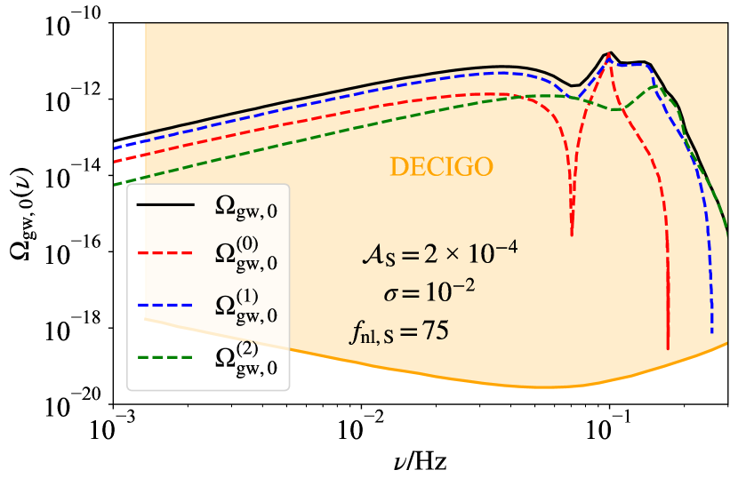
The present-day energy-density fraction spectrum of \acpSIGW is given by Wang et al. (2019)
| (14) |
where the present-day physical energy-density fraction of radiation is with the dimensionless Hubble constant Aghanim et al. (2020). For simplicity, we denote the component of as . In Fig. 1, we depict and with variable , and compare them with the sensitivity curve of \acDECIGO Braglia and Kuroyanagi (2021). It is shown that is enhanced at around , and a large enlarges the spectral amplitude and obviously changes the spectral index.
Angular power spectrum of SIGWs.—Following Refs. Bartolo et al. (2020b); Li et al. (2023a, b), we show that in Eq. (13b), the large-scale leads to the anisotropies in \acpSIGW. Here, we disregard the small-scale inhomogeneities, because the horizon at is extremely small for the present-day observer at , and the observed energy density along a line-of-sight is an average over a quantity of such horizons Bartolo et al. (2020b); Li et al. (2023a, b); Wang et al. (2023a). The observed large-scale in Eq. (13b) is contributed by both the initial density contrast and the Sachs-Wolfe effect Sachs and Wolfe (1967), i.e.,
| (15) |
where we define , and the Bardeen potential follows . Compared with the Sachs-Wolfe effect, the integrated Sachs-Wolfe effect is negligible Bartolo et al. (2020b).
In Eq. (15), we focus on the term , which arises from , indicating the couplings between and . Such couplings can spatially modulate the energy density of \acpSIGW, which were produced by , on superhorizon scales. The large-scale can be obtained from the component of , leading to at the first order. This formula implies that a large amplitude of leads to significant initial inhomogeneities in \acpSIGW. Moreover, higher-order components of are negligible due to .
The observed anisotropies in \acpSIGW, as characterized by a reduced angular power spectrum , arise from the large-scale . With the assumption of the cosmological principle, we define as follows
| (16) |
where represents the coefficients of the spherical harmonic expansion of , i.e.,
| (17) |
Though two with a large angular separation are uncorrelated, serves as a “bridge” to correlate them. Hence, we get . Following a diagrammatic approach, Ref. Li et al. (2023a) presented comprehensive calculations of . The result is given as
| (18) |
where we introduce as a shorthand notation. The first and second terms in the square brackets inherit from Eq. (15) the initial inhomogeneities and the Sachs-Wolfe effect, respectively.
We demonstrate that large anisotropies in \acpSIGW can be generated in our model. We consider that the energy density fraction of the curvaton is small at the time of its decay and the curvature perturbations from curvaton are comparable to those of inflation at while dominant at . Specifically, we quantify these as , resulting in \acPNG through Eqs. (11–12). We further quantify the \acSSR parameters as , leading to in Eq. (9). Therefore, we anticipate the reduced angular power spectrum at around to be
| (19) |
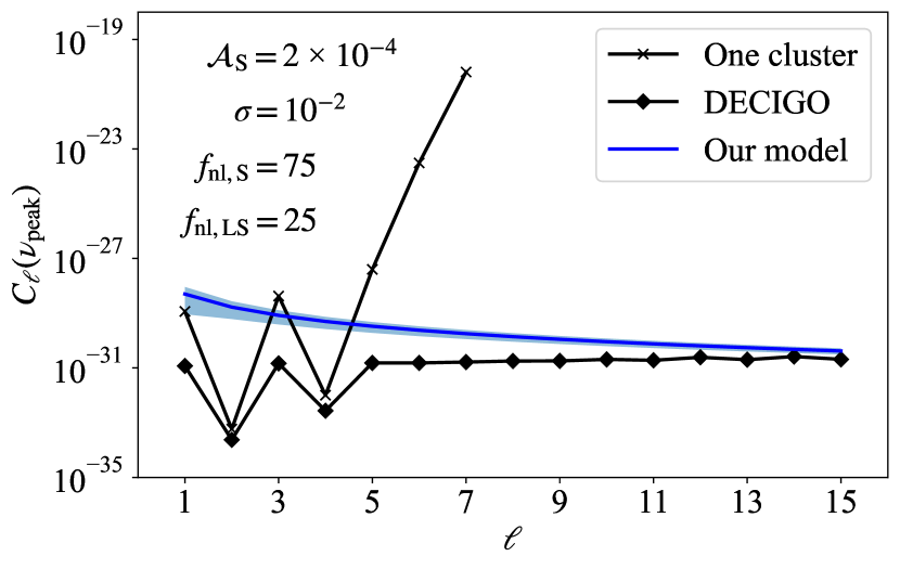
Regarding observations, we define an angular power spectrum as . It could reach , which is potentially observable for future \acGW detectors like \acDECIGO Seto et al. (2001); Kawamura et al. (2021). In Fig. 2, we depict the anticipated at 0.1Hz and compare it with the sensitivity curve of \acDECIGO in the same frequency band Capurri et al. (2023). Moreover, we show an inevitable uncertainty (68% confidence level) due to the cosmic variance in a blue shaded region.
Conclusions and discussion.—In this work, we showed that the large anisotropies in \acpSIGW are generated when the curvaton undergoes \acSSR in the inflaton-curvaton mixed scenario. Introduced by \acSSR, the exponentially amplified curvature perturbations could induce the enhanced energy-density fraction spectrum of \acpSIGW around the resonant frequency. The large \acPNG in this model leads to a large-scale modulation of the energy density of \acpSIGW, resulting in the large anisotropies, i.e., . These anisotropies have potential to be detected by future \acGW detectors like DECIGO.
We may use both the energy-density fraction spectrum and the angular power spectrum of \acpSIGW as complementary probes to study the dynamics of the early universe. The peaked feature in both spectra might serve as a characteristic \acGW signature of this model. The peak width and frequency encode the amplitude and mode of the oscillation of , respectively, while the peak amplitude says the duration of \acSSR, characterized by . Additionally, the imprints of and in and enable us to explore the parameter space of , which carries vital information about the contributions from curvaton to energy density and curvature perturbations. The measurement of all these parameters is helpful in testing various inflationary models.
Different from the existing studies in Refs. Li et al. (2023a), which assumed the scale independence of , our present work considered the scale dependence of . The anisotropies in \acpSIGW offer a remarkable method to measure , which reveals underlying physics of the nonlinear couplings between long- and short-wavelength modes. These anisotropies may initiate a lot of interests in the model-building studies related with the scale-dependent \acPNG. When higher-order \acPNG such as is incorporated Li et al. (2023b), our result in Eq. (19) would not change too much due to when in this model Sasaki et al. (2006); Fonseca and Wands (2012).
The proposed model can lead to efficient production of \acpPBH, shedding new insights on the nature of cold dark matter. Considering the large positive , we roughly estimate the abundance of \acpPBH as Byrnes et al. (2012); Meng et al. (2022)
| (20) | |||||
where stands for the number of relativistic degrees of freedom at the formation time of \acpPBH, is the critical curvature perturbation for gravitational collapse, and denotes the complementary error function with variable . If considering Saikawa and Shirai (2018) and Green et al. (2004), we can obtain at Hz with the parameters adopted in this work. All of cold dark matter could be accounted for by these abundant \acpPBH in the asteroid mass range, which has not been explored by the present observations Carr et al. (2021). However, we should note that the above estimation is sensitively model-dependent.
Acknowledgements.
We appreciate Mr. Jun-Peng Li and Dr. Shi Pi for helpful discussion. This work is partially supported by the National Natural Science Foundation of China (Grant No. 12175243) and the Science Research Grants from the China Manned Space Project with No. CMS-CSST-2021-B01.References
- Aghanim et al. (2020) N. Aghanim et al. (Planck), Astron. Astrophys. 641, A6 (2020), [Erratum: Astron.Astrophys. 652, C4 (2021)], arXiv:1807.06209 [astro-ph.CO] .
- Akrami et al. (2020a) Y. Akrami et al. (Planck), Astron. Astrophys. 641, A10 (2020a), arXiv:1807.06211 [astro-ph.CO] .
- Bartolo et al. (2018) N. Bartolo, A. Hoseinpour, G. Orlando, S. Matarrese, and M. Zarei, Phys. Rev. D 98, 023518 (2018), arXiv:1804.06298 [gr-qc] .
- Flauger and Weinberg (2019) R. Flauger and S. Weinberg, Phys. Rev. D 99, 123030 (2019), arXiv:1906.04853 [hep-th] .
- Bartolo et al. (2022) N. Bartolo et al. (LISA Cosmology Working Group), JCAP 11, 009 (2022), arXiv:2201.08782 [astro-ph.CO] .
- Agazie et al. (2023a) G. Agazie et al. (NANOGrav), Astrophys. J. Lett. 951, L8 (2023a), arXiv:2306.16213 [astro-ph.HE] .
- Antoniadis et al. (2023) J. Antoniadis et al. (EPTA), (2023), arXiv:2306.16214 [astro-ph.HE] .
- Reardon et al. (2023) D. J. Reardon et al., Astrophys. J. Lett. 951, L6 (2023), arXiv:2306.16215 [astro-ph.HE] .
- Xu et al. (2023) H. Xu et al., Res. Astron. Astrophys. 23, 075024 (2023), arXiv:2306.16216 [astro-ph.HE] .
- Bartolo et al. (2019) N. Bartolo, D. Bertacca, S. Matarrese, M. Peloso, A. Ricciardone, A. Riotto, and G. Tasinato, Phys. Rev. D 100, 121501 (2019), arXiv:1908.00527 [astro-ph.CO] .
- Bartolo et al. (2020a) N. Bartolo, D. Bertacca, S. Matarrese, M. Peloso, A. Ricciardone, A. Riotto, and G. Tasinato, Phys. Rev. D 102, 023527 (2020a), arXiv:1912.09433 [astro-ph.CO] .
- Bartolo et al. (2020b) N. Bartolo, D. Bertacca, V. De Luca, G. Franciolini, S. Matarrese, M. Peloso, A. Ricciardone, A. Riotto, and G. Tasinato, JCAP 02, 028 (2020b), arXiv:1909.12619 [astro-ph.CO] .
- Li et al. (2023a) J.-P. Li, S. Wang, Z.-C. Zhao, and K. Kohri, (2023a), arXiv:2305.19950 [astro-ph.CO] .
- Li et al. (2023b) J.-P. Li, S. Wang, Z.-C. Zhao, and K. Kohri, (2023b), arXiv:2309.07792 [astro-ph.CO] .
- Wang et al. (2023a) S. Wang, Z.-C. Zhao, J.-P. Li, and Q.-H. Zhu, (2023a), arXiv:2307.00572 [astro-ph.CO] .
- Dimastrogiovanni et al. (2023) E. Dimastrogiovanni, M. Fasiello, A. Malhotra, and G. Tasinato, JCAP 01, 018 (2023), arXiv:2205.05644 [astro-ph.CO] .
- Contaldi (2017) C. R. Contaldi, Phys. Lett. B 771, 9 (2017), arXiv:1609.08168 [astro-ph.CO] .
- Jenkins et al. (2019a) A. C. Jenkins, R. O’Shaughnessy, M. Sakellariadou, and D. Wysocki, Phys. Rev. Lett. 122, 111101 (2019a), arXiv:1810.13435 [astro-ph.CO] .
- Jenkins et al. (2018) A. C. Jenkins, M. Sakellariadou, T. Regimbau, and E. Slezak, Phys. Rev. D 98, 063501 (2018), arXiv:1806.01718 [astro-ph.CO] .
- Jenkins and Sakellariadou (2019) A. C. Jenkins and M. Sakellariadou, Phys. Rev. D 100, 063508 (2019), arXiv:1902.07719 [astro-ph.CO] .
- Jenkins et al. (2019b) A. C. Jenkins, J. D. Romano, and M. Sakellariadou, Phys. Rev. D 100, 083501 (2019b), arXiv:1907.06642 [astro-ph.CO] .
- Bertacca et al. (2020) D. Bertacca, A. Ricciardone, N. Bellomo, A. C. Jenkins, S. Matarrese, A. Raccanelli, T. Regimbau, and M. Sakellariadou, Phys. Rev. D 101, 103513 (2020), arXiv:1909.11627 [astro-ph.CO] .
- Cusin et al. (2017) G. Cusin, C. Pitrou, and J.-P. Uzan, Phys. Rev. D96, 103019 (2017), arXiv:1704.06184 [astro-ph.CO] .
- Cusin et al. (2018a) G. Cusin, C. Pitrou, and J.-P. Uzan, Phys. Rev. D97, 123527 (2018a), arXiv:1711.11345 [astro-ph.CO] .
- Cusin et al. (2018b) G. Cusin, I. Dvorkin, C. Pitrou, and J.-P. Uzan, Phys. Rev. Lett. 120, 231101 (2018b), arXiv:1803.03236 [astro-ph.CO] .
- Cusin et al. (2020) G. Cusin, I. Dvorkin, C. Pitrou, and J.-P. Uzan, Mon. Not. Roy. Astron. Soc. 493, L1 (2020), arXiv:1904.07757 [astro-ph.CO] .
- Cusin et al. (2019) G. Cusin, I. Dvorkin, C. Pitrou, and J.-P. Uzan, Phys. Rev. D 100, 063004 (2019), arXiv:1904.07797 [astro-ph.CO] .
- Wang et al. (2022) S. Wang, V. Vardanyan, and K. Kohri, Phys. Rev. D 106, 123511 (2022), arXiv:2107.01935 [gr-qc] .
- Mukherjee and Silk (2020) S. Mukherjee and J. Silk, Mon. Not. Roy. Astron. Soc. 491, 4690 (2020), arXiv:1912.07657 [gr-qc] .
- Bavera et al. (2022) S. S. Bavera, G. Franciolini, G. Cusin, A. Riotto, M. Zevin, and T. Fragos, Astron. Astrophys. 660, A26 (2022), arXiv:2109.05836 [astro-ph.CO] .
- Bellomo et al. (2021) N. Bellomo, D. Bertacca, A. C. Jenkins, S. Matarrese, A. Raccanelli, T. Regimbau, A. Ricciardone, and M. Sakellariadou, (2021), arXiv:2110.15059 [gr-qc] .
- Pitrou et al. (2020) C. Pitrou, G. Cusin, and J.-P. Uzan, Phys. Rev. D 101, 081301 (2020), arXiv:1910.04645 [astro-ph.CO] .
- Cañas Herrera et al. (2020) G. Cañas Herrera, O. Contigiani, and V. Vardanyan, Phys. Rev. D 102, 043513 (2020), arXiv:1910.08353 [astro-ph.CO] .
- Geller et al. (2018) M. Geller, A. Hook, R. Sundrum, and Y. Tsai, Phys. Rev. Lett. 121, 201303 (2018), arXiv:1803.10780 [hep-ph] .
- Jenkins and Sakellariadou (2018) A. C. Jenkins and M. Sakellariadou, Phys. Rev. D 98, 063509 (2018), arXiv:1802.06046 [astro-ph.CO] .
- Kuroyanagi et al. (2017) S. Kuroyanagi, K. Takahashi, N. Yonemaru, and H. Kumamoto, Phys. Rev. D 95, 043531 (2017), arXiv:1604.00332 [astro-ph.CO] .
- Olmez et al. (2012) S. Olmez, V. Mandic, and X. Siemens, JCAP 07, 009 (2012), arXiv:1106.5555 [astro-ph.CO] .
- Dimastrogiovanni et al. (2022) E. Dimastrogiovanni, M. Fasiello, A. Malhotra, P. D. Meerburg, and G. Orlando, JCAP 02, 040 (2022), arXiv:2109.03077 [astro-ph.CO] .
- Valbusa Dall’Armi et al. (2023a) L. Valbusa Dall’Armi, A. Mierna, S. Matarrese, and A. Ricciardone, (2023a), arXiv:2307.11043 [astro-ph.CO] .
- Cui et al. (2023) Y. Cui, S. Kumar, R. Sundrum, and Y. Tsai, (2023), arXiv:2307.10360 [astro-ph.CO] .
- Adshead et al. (2021a) P. Adshead, N. Afshordi, E. Dimastrogiovanni, M. Fasiello, E. A. Lim, and G. Tasinato, Phys. Rev. D 103, 023532 (2021a), arXiv:2004.06619 [astro-ph.CO] .
- Dimastrogiovanni et al. (2020) E. Dimastrogiovanni, M. Fasiello, and G. Tasinato, Phys. Rev. Lett. 124, 061302 (2020), arXiv:1906.07204 [astro-ph.CO] .
- Jeong and Kamionkowski (2012) D. Jeong and M. Kamionkowski, Phys. Rev. Lett. 108, 251301 (2012), arXiv:1203.0302 [astro-ph.CO] .
- Liu et al. (2021) J. Liu, R.-G. Cai, and Z.-K. Guo, Phys. Rev. Lett. 126, 141303 (2021), arXiv:2010.03225 [astro-ph.CO] .
- Li et al. (2022) Y. Li, F. P. Huang, X. Wang, and X. Zhang, Phys. Rev. D 105, 083527 (2022), arXiv:2112.01409 [astro-ph.CO] .
- Domcke et al. (2020) V. Domcke, R. Jinno, and H. Rubira, JCAP 06, 046 (2020), arXiv:2002.11083 [astro-ph.CO] .
- Jinno et al. (2021) R. Jinno, T. Konstandin, H. Rubira, and J. van de Vis, JCAP 12, 019 (2021), arXiv:2108.11947 [astro-ph.CO] .
- Kumar et al. (2021) S. Kumar, R. Sundrum, and Y. Tsai, JHEP 11, 107 (2021), arXiv:2102.05665 [astro-ph.CO] .
- Racco and Poletti (2023) D. Racco and D. Poletti, JCAP 04, 054 (2023), arXiv:2212.06602 [astro-ph.CO] .
- Bethke et al. (2013) L. Bethke, D. G. Figueroa, and A. Rajantie, Phys. Rev. Lett. 111, 011301 (2013), arXiv:1304.2657 [astro-ph.CO] .
- Bethke et al. (2014) L. Bethke, D. G. Figueroa, and A. Rajantie, JCAP 06, 047 (2014), arXiv:1309.1148 [astro-ph.CO] .
- Valbusa Dall’Armi et al. (2023b) L. Valbusa Dall’Armi, A. Nishizawa, A. Ricciardone, and S. Matarrese, Phys. Rev. Lett. 131, 041401 (2023b), arXiv:2301.08205 [astro-ph.CO] .
- Ananda et al. (2007) K. N. Ananda, C. Clarkson, and D. Wands, Phys. Rev. D75, 123518 (2007), arXiv:gr-qc/0612013 [gr-qc] .
- Baumann et al. (2007) D. Baumann, P. J. Steinhardt, K. Takahashi, and K. Ichiki, Phys. Rev. D76, 084019 (2007), arXiv:hep-th/0703290 [hep-th] .
- Espinosa et al. (2018) J. R. Espinosa, D. Racco, and A. Riotto, JCAP 09, 012 (2018), arXiv:1804.07732 [hep-ph] .
- Kohri and Terada (2018) K. Kohri and T. Terada, Phys. Rev. D97, 123532 (2018), arXiv:1804.08577 [gr-qc] .
- Mollerach et al. (2004) S. Mollerach, D. Harari, and S. Matarrese, Phys. Rev. D69, 063002 (2004), arXiv:astro-ph/0310711 [astro-ph] .
- Assadullahi and Wands (2010) H. Assadullahi and D. Wands, Phys. Rev. D81, 023527 (2010), arXiv:0907.4073 [astro-ph.CO] .
- Domènech (2021) G. Domènech, Universe 7, 398 (2021), arXiv:2109.01398 [gr-qc] .
- Valbusa Dall’Armi et al. (2021) L. Valbusa Dall’Armi, A. Ricciardone, N. Bartolo, D. Bertacca, and S. Matarrese, Phys. Rev. D 103, 023522 (2021), arXiv:2007.01215 [astro-ph.CO] .
- Auclair et al. (2023) P. Auclair et al. (LISA Cosmology Working Group), Living Rev. Rel. 26, 5 (2023), arXiv:2204.05434 [astro-ph.CO] .
- Ünal et al. (2021) C. Ünal, E. D. Kovetz, and S. P. Patil, Phys. Rev. D 103, 063519 (2021), arXiv:2008.11184 [astro-ph.CO] .
- Malhotra et al. (2021) A. Malhotra, E. Dimastrogiovanni, M. Fasiello, and M. Shiraishi, JCAP 03, 088 (2021), arXiv:2012.03498 [astro-ph.CO] .
- Carr et al. (2021) B. Carr, K. Kohri, Y. Sendouda, and J. Yokoyama, Rept. Prog. Phys. 84, 116902 (2021), arXiv:2002.12778 [astro-ph.CO] .
- Maldacena (2003) J. M. Maldacena, JHEP 05, 013 (2003), arXiv:astro-ph/0210603 .
- Bartolo et al. (2004a) N. Bartolo, E. Komatsu, S. Matarrese, and A. Riotto, Phys. Rept. 402, 103 (2004a), arXiv:astro-ph/0406398 .
- Allen et al. (1987) T. J. Allen, B. Grinstein, and M. B. Wise, Phys. Lett. B 197, 66 (1987).
- Bartolo et al. (2002) N. Bartolo, S. Matarrese, and A. Riotto, Phys. Rev. D 65, 103505 (2002), arXiv:hep-ph/0112261 .
- Acquaviva et al. (2003) V. Acquaviva, N. Bartolo, S. Matarrese, and A. Riotto, Nucl. Phys. B 667, 119 (2003), arXiv:astro-ph/0209156 .
- Bernardeau and Uzan (2002) F. Bernardeau and J.-P. Uzan, Phys. Rev. D 66, 103506 (2002), arXiv:hep-ph/0207295 .
- Chen et al. (2007) X. Chen, M.-x. Huang, S. Kachru, and G. Shiu, JCAP 01, 002 (2007), arXiv:hep-th/0605045 .
- Chen (2010) X. Chen, Adv. Astron. 2010, 638979 (2010), arXiv:1002.1416 [astro-ph.CO] .
- Choudhury et al. (2023) S. Choudhury, A. Karde, K. Dey, S. Panda, and M. Sami, (2023), arXiv:2310.11034 [astro-ph.CO] .
- Agazie et al. (2023b) G. Agazie et al. (NANOGrav), (2023b), arXiv:2306.16221 [astro-ph.HE] .
- Abbott et al. (2017) B. P. Abbott et al. (LIGO Scientific, Virgo), Phys. Rev. Lett. 118, 121102 (2017), arXiv:1612.02030 [gr-qc] .
- Abbott et al. (2019) B. P. Abbott et al. (LIGO Scientific, Virgo), Phys. Rev. D 100, 062001 (2019), arXiv:1903.08844 [gr-qc] .
- Abbott et al. (2021) R. Abbott et al. (KAGRA, Virgo, LIGO Scientific), Phys. Rev. D 104, 022005 (2021), arXiv:2103.08520 [gr-qc] .
- Cai et al. (2018a) Y.-F. Cai, X. Tong, D.-G. Wang, and S.-F. Yan, Phys. Rev. Lett. 121, 081306 (2018a), arXiv:1805.03639 [astro-ph.CO] .
- Cai et al. (2019) Y.-F. Cai, C. Chen, X. Tong, D.-G. Wang, and S.-F. Yan, Phys. Rev. D 100, 043518 (2019), arXiv:1902.08187 [astro-ph.CO] .
- Chen and Cai (2019) C. Chen and Y.-F. Cai, JCAP 10, 068 (2019), arXiv:1908.03942 [astro-ph.CO] .
- Chen et al. (2020) C. Chen, X.-H. Ma, and Y.-F. Cai, Phys. Rev. D 102, 063526 (2020), arXiv:2003.03821 [astro-ph.CO] .
- Langlois and Vernizzi (2004) D. Langlois and F. Vernizzi, Phys. Rev. D 70, 063522 (2004), arXiv:astro-ph/0403258 .
- Ferrer et al. (2004) F. Ferrer, S. Rasanen, and J. Valiviita, JCAP 10, 010 (2004), arXiv:astro-ph/0407300 .
- Langlois et al. (2008) D. Langlois, F. Vernizzi, and D. Wands, JCAP 12, 004 (2008), arXiv:0809.4646 [astro-ph] .
- Fonseca and Wands (2012) J. Fonseca and D. Wands, JCAP 06, 028 (2012), arXiv:1204.3443 [astro-ph.CO] .
- Chluba et al. (2019) J. Chluba et al., Bull. Am. Astron. Soc. 51, 184 (2019), arXiv:1903.04218 [astro-ph.CO] .
- Jeong et al. (2014) D. Jeong, J. Pradler, J. Chluba, and M. Kamionkowski, Phys. Rev. Lett. 113, 061301 (2014), arXiv:1403.3697 [astro-ph.CO] .
- Nakama et al. (2014) T. Nakama, T. Suyama, and J. Yokoyama, Phys. Rev. Lett. 113, 061302 (2014), arXiv:1403.5407 [astro-ph.CO] .
- Inomata et al. (2016) K. Inomata, M. Kawasaki, and Y. Tada, Phys. Rev. D 94, 043527 (2016), arXiv:1605.04646 [astro-ph.CO] .
- Allahverdi et al. (2020) R. Allahverdi et al., (2020), 10.21105/astro.2006.16182, arXiv:2006.16182 [astro-ph.CO] .
- Gow et al. (2021) A. D. Gow, C. T. Byrnes, P. S. Cole, and S. Young, JCAP 02, 002 (2021), arXiv:2008.03289 [astro-ph.CO] .
- Franciolini and Urbano (2022) G. Franciolini and A. Urbano, Phys. Rev. D 106, 123519 (2022), arXiv:2207.10056 [astro-ph.CO] .
- Franciolini et al. (2022) G. Franciolini, I. Musco, P. Pani, and A. Urbano, Phys. Rev. D 106, 123526 (2022), arXiv:2209.05959 [astro-ph.CO] .
- Wang et al. (2023b) X. Wang, Y.-l. Zhang, R. Kimura, and M. Yamaguchi, Sci. China Phys. Mech. Astron. 66, 260462 (2023b), arXiv:2209.12911 [astro-ph.CO] .
- Sasaki et al. (2018) M. Sasaki, T. Suyama, T. Tanaka, and S. Yokoyama, Class. Quant. Grav. 35, 063001 (2018), arXiv:1801.05235 [astro-ph.CO] .
- Carr and Kuhnel (2020) B. Carr and F. Kuhnel, Ann. Rev. Nucl. Part. Sci. 70, 355 (2020), arXiv:2006.02838 [astro-ph.CO] .
- Linde and Mukhanov (1997) A. D. Linde and V. F. Mukhanov, Phys. Rev. D 56, R535 (1997), arXiv:astro-ph/9610219 .
- Lyth and Wands (2002) D. H. Lyth and D. Wands, Phys. Lett. B 524, 5 (2002), arXiv:hep-ph/0110002 .
- Enqvist and Sloth (2002) K. Enqvist and M. S. Sloth, Nucl. Phys. B 626, 395 (2002), arXiv:hep-ph/0109214 .
- Lyth et al. (2003) D. H. Lyth, C. Ungarelli, and D. Wands, Phys. Rev. D 67, 023503 (2003), arXiv:astro-ph/0208055 .
- Moroi and Takahashi (2001) T. Moroi and T. Takahashi, Phys. Lett. B 522, 215 (2001), [Erratum: Phys.Lett.B 539, 303–303 (2002)], arXiv:hep-ph/0110096 .
- Bartolo et al. (2004b) N. Bartolo, S. Matarrese, and A. Riotto, Phys. Rev. D 69, 043503 (2004b), arXiv:hep-ph/0309033 .
- Sasaki et al. (2006) M. Sasaki, J. Valiviita, and D. Wands, Phys. Rev. D 74, 103003 (2006), arXiv:astro-ph/0607627 .
- Huang (2008) Q.-G. Huang, Phys. Lett. B 669, 260 (2008), arXiv:0801.0467 [hep-th] .
- Beltran (2008) M. Beltran, Phys. Rev. D 78, 023530 (2008), arXiv:0804.1097 [astro-ph] .
- Enqvist and Nurmi (2005) K. Enqvist and S. Nurmi, JCAP 10, 013 (2005), arXiv:astro-ph/0508573 .
- Malik and Lyth (2006) K. A. Malik and D. H. Lyth, JCAP 09, 008 (2006), arXiv:astro-ph/0604387 .
- Pi and Sasaki (2021) S. Pi and M. Sasaki, (2021), arXiv:2112.12680 [astro-ph.CO] .
- Malhotra et al. (2023) A. Malhotra, E. Dimastrogiovanni, G. Domènech, M. Fasiello, and G. Tasinato, Phys. Rev. D 107, 103502 (2023), arXiv:2212.10316 [gr-qc] .
- Silverstein and Tong (2004) E. Silverstein and D. Tong, Phys. Rev. D 70, 103505 (2004), arXiv:hep-th/0310221 .
- Alishahiha et al. (2004) M. Alishahiha, E. Silverstein, and D. Tong, Phys. Rev. D 70, 123505 (2004), arXiv:hep-th/0404084 .
- Armendariz-Picon et al. (1999) C. Armendariz-Picon, T. Damour, and V. F. Mukhanov, Phys. Lett. B 458, 209 (1999), arXiv:hep-th/9904075 .
- Garriga and Mukhanov (1999) J. Garriga and V. F. Mukhanov, Phys. Lett. B 458, 219 (1999), arXiv:hep-th/9904176 .
- Achucarro et al. (2011) A. Achucarro, J.-O. Gong, S. Hardeman, G. A. Palma, and S. P. Patil, JCAP 01, 030 (2011), arXiv:1010.3693 [hep-ph] .
- Achúcarro et al. (2014) A. Achúcarro, V. Atal, P. Ortiz, and J. Torrado, Phys. Rev. D 89, 103006 (2014), arXiv:1311.2552 [astro-ph.CO] .
- Pi et al. (2018) S. Pi, Y.-l. Zhang, Q.-G. Huang, and M. Sasaki, JCAP 05, 042 (2018), arXiv:1712.09896 [astro-ph.CO] .
- Harry and (for the LIGO Scientific Collaboration) G. M. Harry and (for the LIGO Scientific Collaboration), Classical and Quantum Gravity 27, 084006 (2010).
- Acernese et al. (2015) F. Acernese et al. (VIRGO), Class. Quant. Grav. 32, 024001 (2015), arXiv:1408.3978 [gr-qc] .
- Somiya (2012) K. Somiya (KAGRA), Class. Quant. Grav. 29, 124007 (2012), arXiv:1111.7185 [gr-qc] .
- Hild et al. (2011) S. Hild et al., Class. Quant. Grav. 28, 094013 (2011), arXiv:1012.0908 [gr-qc] .
- Thorpe et al. (2019) J. I. Thorpe et al., in Bulletin of the American Astronomical Society, Vol. 51 (2019) p. 77, arXiv:1907.06482 [astro-ph.IM] .
- Smith et al. (2019) T. L. Smith, T. L. Smith, R. R. Caldwell, and R. Caldwell, Phys. Rev. D 100, 104055 (2019), [Erratum: Phys.Rev.D 105, 029902 (2022)], arXiv:1908.00546 [astro-ph.CO] .
- Hu and Wu (2017) W.-R. Hu and Y.-L. Wu, Natl. Sci. Rev. 4, 685 (2017).
- Carilli and Rawlings (2004) C. L. Carilli and S. Rawlings, New Astron. Rev. 48, 979 (2004), arXiv:astro-ph/0409274 .
- Seto et al. (2001) N. Seto, S. Kawamura, and T. Nakamura, Phys. Rev. Lett. 87, 221103 (2001), arXiv:astro-ph/0108011 .
- Kawamura et al. (2021) S. Kawamura et al., PTEP 2021, 05A105 (2021), arXiv:2006.13545 [gr-qc] .
- Mukhanov (1988) V. F. Mukhanov, Sov. Phys. JETP 67, 1297 (1988).
- Sasaki (1986) M. Sasaki, Prog. Theor. Phys. 76, 1036 (1986).
- Sasaki and Stewart (1996) M. Sasaki and E. D. Stewart, Prog. Theor. Phys. 95, 71 (1996), arXiv:astro-ph/9507001 .
- Starobinsky (1985) A. A. Starobinsky, JETP Lett. 42, 152 (1985).
- Wands et al. (2000) D. Wands, K. A. Malik, D. H. Lyth, and A. R. Liddle, Phys. Rev. D 62, 043527 (2000), arXiv:astro-ph/0003278 .
- Lyth et al. (2005) D. H. Lyth, K. A. Malik, and M. Sasaki, JCAP 05, 004 (2005), arXiv:astro-ph/0411220 .
- Kohri et al. (2013) K. Kohri, C.-M. Lin, and T. Matsuda, Phys. Rev. D 87, 103527 (2013), arXiv:1211.2371 [hep-ph] .
- Tada and Yokoyama (2015) Y. Tada and S. Yokoyama, Phys. Rev. D 91, 123534 (2015), arXiv:1502.01124 [astro-ph.CO] .
- Komatsu and Spergel (2001) E. Komatsu and D. N. Spergel, Phys. Rev. D 63, 063002 (2001), arXiv:astro-ph/0005036 .
- Akrami et al. (2020b) Y. Akrami et al. (Planck), Astron. Astrophys. 641, A9 (2020b), arXiv:1905.05697 [astro-ph.CO] .
- Maggiore (2000) M. Maggiore, Phys. Rept. 331, 283 (2000), arXiv:gr-qc/9909001 .
- Adshead et al. (2021b) P. Adshead, K. D. Lozanov, and Z. J. Weiner, JCAP 10, 080 (2021b), arXiv:2105.01659 [astro-ph.CO] .
- Ragavendra (2022) H. V. Ragavendra, Phys. Rev. D 105, 063533 (2022), arXiv:2108.04193 [astro-ph.CO] .
- Abe et al. (2023) K. T. Abe, R. Inui, Y. Tada, and S. Yokoyama, JCAP 05, 044 (2023), arXiv:2209.13891 [astro-ph.CO] .
- Cai et al. (2018b) R.-g. Cai, S. Pi, and M. Sasaki, (2018b), arXiv:1810.11000 [astro-ph.CO] .
- Unal (2019) C. Unal, Phys. Rev. D99, 041301 (2019), arXiv:1811.09151 [astro-ph.CO] .
- Atal and Domènech (2021) V. Atal and G. Domènech, JCAP 06, 001 (2021), arXiv:2103.01056 [astro-ph.CO] .
- Ragavendra et al. (2021) H. V. Ragavendra, P. Saha, L. Sriramkumar, and J. Silk, Phys. Rev. D 103, 083510 (2021), arXiv:2008.12202 [astro-ph.CO] .
- Yuan and Huang (2021) C. Yuan and Q.-G. Huang, Phys. Lett. B 821, 136606 (2021), arXiv:2007.10686 [astro-ph.CO] .
- Yuan et al. (2023) C. Yuan, D.-S. Meng, and Q.-G. Huang, (2023), arXiv:2308.07155 [astro-ph.CO] .
- Garcia-Saenz et al. (2023) S. Garcia-Saenz, L. Pinol, S. Renaux-Petel, and D. Werth, JCAP 03, 057 (2023), arXiv:2207.14267 [astro-ph.CO] .
- Zhang (2022) F. Zhang, Phys. Rev. D 105, 063539 (2022), arXiv:2112.10516 [gr-qc] .
- Domènech and Sasaki (2018) G. Domènech and M. Sasaki, Phys. Rev. D 97, 023521 (2018), arXiv:1709.09804 [gr-qc] .
- Garcia-Bellido et al. (2017) J. Garcia-Bellido, M. Peloso, and C. Unal, JCAP 1709, 013 (2017), arXiv:1707.02441 [astro-ph.CO] .
- Nakama et al. (2017) T. Nakama, J. Silk, and M. Kamionkowski, Phys. Rev. D 95, 043511 (2017), arXiv:1612.06264 [astro-ph.CO] .
- Wang et al. (2019) S. Wang, T. Terada, and K. Kohri, Phys. Rev. D99, 103531 (2019), [erratum: Phys. Rev.D101,no.6,069901(2020)], arXiv:1903.05924 [astro-ph.CO] .
- Braglia and Kuroyanagi (2021) M. Braglia and S. Kuroyanagi, Phys. Rev. D 104, 123547 (2021), arXiv:2106.03786 [astro-ph.CO] .
- Sachs and Wolfe (1967) R. K. Sachs and A. M. Wolfe, Astrophys. J. 147, 73 (1967).
- Capurri et al. (2023) G. Capurri, A. Lapi, L. Boco, and C. Baccigalupi, Astrophys. J. 943, 72 (2023), arXiv:2212.06162 [gr-qc] .
- Byrnes et al. (2012) C. T. Byrnes, E. J. Copeland, and A. M. Green, Phys. Rev. D 86, 043512 (2012), arXiv:1206.4188 [astro-ph.CO] .
- Meng et al. (2022) D.-S. Meng, C. Yuan, and Q.-G. Huang, Phys. Rev. D 106, 063508 (2022), arXiv:2207.07668 [astro-ph.CO] .
- Saikawa and Shirai (2018) K. Saikawa and S. Shirai, JCAP 1805, 035 (2018), arXiv:1803.01038 [hep-ph] .
- Green et al. (2004) A. M. Green, A. R. Liddle, K. A. Malik, and M. Sasaki, Phys. Rev. D 70, 041502 (2004), arXiv:astro-ph/0403181 .