Pre-training LiDAR-based 3D Object Detectors through Colorization

Abstract

Accurate 3D object detection and understanding for self-driving cars heavily relies on LiDAR point clouds, necessitating large amounts of labeled data to train. In this work, we introduce an innovative pre-training approach, Grounded Point Colorization (GPC), to bridge the gap between data and labels by teaching the model to colorize LiDAR point clouds, equipping it with valuable semantic cues. To tackle challenges arising from color variations and selection bias, we incorporate color as “context" by providing ground-truth colors as hints during colorization. Experimental results on the KITTI and Waymo datasets demonstrate GPC’s remarkable effectiveness. Even with limited labeled data, GPC significantly improves fine-tuning performance; notably, on just 20% of the KITTI dataset, GPC outperforms training from scratch with the entire dataset. In sum, we introduce a fresh perspective on pre-training for 3D object detection, aligning the objective with the model’s intended role and ultimately advancing the accuracy and efficiency of 3D object detection for autonomous vehicles.

1 Introduction

Detecting objects such as vehicles and pedestrians in 3D is crucial for self-driving cars to operate safely. Mainstream 3D object detectors (Shi et al., 2019; 2020b; Zhu et al., 2020; He et al., 2020a) take LiDAR point clouds as input, which provide precise 3D signals of the surrounding environment. However, training a detector needs a lot of labeled data. The expensive process of curating annotated data has motivated the community to investigate model pre-training using unlabeled data that can be collected easily. Most of the existing pre-training methods are built upon contrastive learning (Yin et al., 2022; Xie et al., 2020; Zhang et al., 2021; Huang et al., 2021; Liang et al., 2021), inspired by its success in 2D recognition (Chen et al., 2020a; He et al., 2020b). The key novelties, however, are often limited to how the positive and negative data pairs are constructed. This paper attempts to go beyond contrastive learning by providing a new perspective on pre-training 3D object detectors.

We rethink pre-training’s role in how it could facilitate the downstream fine-tuning with labeled data. A labeled example of 3D object detection comprises a point cloud and a set of bounding boxes. While the format is typical, there is no explicit connection between the input data and labels. We argue that a pre-training approach should help bridge these two pieces of information to facilitate fine-tuning.

How can we go from point clouds to bounding boxes without human supervision? One intuitive way is to first segment the point cloud, followed by rules to read out the bounding box of each segment. The closer the segments match the objects of interest, the higher their qualities are. While a raw LiDAR point cloud may not provide clear semantic cues to segment objects, the color image collected along with it does. In color images, each object instance often possesses a coherent color and has a sharp contrast to the background. This information has been widely used in image segmentation (Li & Chen, 2015; Liu et al., 2011; Adams & Bischof, 1994) before machine learning-based methods take over. We hypothesize that by learning to predict the pixel color each LiDAR point is projected to, the pre-trained LiDAR-based model backbone will be equipped with the semantic cues that facilitate the subsequent fine-tuning for 3D object detection. To this end, we propose pre-training a LiDAR-based 3D object detector by learning to colorize LiDAR point clouds. Such an objective makes the pre-training procedure fairly straightforward, which we see as a key strength. Taking models that use point-based backbones like PointNet++ (Qi et al., 2017b; a) as an example, pre-training becomes solving a point-wise regression problem (for predicting the RGB values).

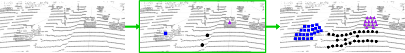
Figure 1: Illustration of the proposed Grounded Point Colorization (GPC). We pre-train the detector backbone by colorization (left to right), taking the hints on a seed set of points (middle) to overcome the inherent color variation. We show that the middle step is the key to learning the semantic cues of objects from colors.

That said, the ground-truth colors of a LiDAR point cloud contain inherent variations. For example, the same car model (hence the same point cloud) can have multiple color options; the same street scene (hence the same point cloud) can be pictured with different colors depending on the time and weather. When selection bias occurs in the collected data (e.g., only a few instances of the variations are collected), the model may learn to capture the bias, degrading its transferability. When the data is well collected to cover all variations without selection bias, the model may learn to predict the average color, downgrading the semantic cues (e.g., contrast). Such a dilemma seems to paint a grim picture of using colors to supervise pre-training. In fact, the second issue is reminiscent of the “noise” term in the well-known bias-variance decomposition (Hastie et al., 2009), which cannot be reduced by machine learning algorithms. The solution must come from a better way to use the data.

Based on this insight, we propose a fairly simple but effective refinement to how we leverage color. Instead of using color solely as the supervised signal, we use it as “context” to ground the colorization process on the inherent color variation. We realize this idea by providing ground-truth colors to a seed set of LiDAR points as “hints” for colorization. (Fig. 1 gives an illustration.) On the one hand, this contextual information reduces the color variations on the remaining points and, in turn, increases the mutual information between the remaining points and the ground-truth colors to supervise pre-training. On the other hand, when selection bias exists, this contextual information directly captures it and offers it as a “shortcut” to the colorization process. This could reduce the tendency of a model to (re-)learn this bias (Lu, 2022; Clark et al., 2019; Cadene et al., 2019), enabling it to focus on the semantic cues useful for 3D object detection. After all, what we hope the model learns is not the exact color of each point but which subset of points should possess the same color and be segmented together. By providing the ground-truth colors to a seed set of points during the colorization process, we concentrate the model backbone on discovering with which points each seed point should share its color, aligning the pre-training objective to its desired role.

We implement our idea, which we name Grounded Point Colorization (GPC), by introducing another point-based model (e.g., PointNet++) on top of the detector backbone. This could be seen as the projection head commonly added in contrastive learning (Chen et al., 2020a); Fig. 2 provides an illustration. While the detector backbone takes only the LiDAR point cloud as input, the projection head takes both the output embeddings of the LiDAR points and the ground-truth colors of a seed set of points as input and is in charge of filling in the missing colors grounded on the seed points. This leaves the detector backbone with a more dedicated task — producing output embeddings with clear semantic cues about which subset of points should be colored (i.e., segmented) together.

We conduct extensive experiments to validate GPC, using the KITTI (Geiger et al., 2012) and Waymo (Sun et al., 2020) datasets. We show that GPC can effectively boost the fine-tuning performance, especially on the labeled-data-scarce settings. For example, with GPC, fine-tuning on 20% KITTI is already better than training 100% from scratch. Fine-tuning using the whole dataset still brings a notable $1.2\%$ gain on overall AP, outperforming existing baselines.

Our contributions are three-fold. First, we propose pre-training by colorizing the LiDAR points — a novel approach different from the commonly used contrastive learning methods. Second, we identify the intrinsic difficulty of using color as the supervised signal and propose a simple yet well-founded and effective treatment. Third, we conduct extensive empirical studies to validate our approach.

2 Related Work

LiDAR-based 3D object detectors.

Existing methods can be roughly categorized into two groups based on their feature extractors. Point-based methods (Shi et al., 2019; Zhang et al., 2022b; Qi et al., 2019; Fan et al., 2022; Yang et al., 2020) extract features for each LiDAR point. Voxel-based methods (Shi et al., 2020a; Yin et al., 2021; Yan et al., 2018; Lang et al., 2019) extract features on grid locations, resulting in a feature tensor. In this paper, we focus on point-based 3D object detectors.

SSL on point clouds by contrastive learning.

Self-supervised learning (SSL) seeks to build feature representations without human annotations. The main branch of work is based on contrastive learning (Chen et al., 2020a; Chen & He, 2021; He et al., 2020b; Chen et al., 2020b; Grill et al., 2020; Henaff, 2020; Tian et al., 2020). For example, Zhang et al. (2021); Huang et al. (2021) treat each point cloud as an instance and learn the representation using contrastive learning. Liang et al. (2021); Xie et al. (2020); Yin et al. (2022) build point features by contrasting them across different regions in different scenes. The challenge is how to construct data pairs to contrast, which often needs extra information or ad hoc design such as spatial-temporal information (Huang et al., 2021) and ground planes (Yin et al., 2022). Our approach goes beyond contrastive learning for SSL on point clouds.

SSL on point clouds by reconstruction.

Inspired by natural languages processing (Devlin et al., 2018; Raffel et al., 2020) and image understanding (Zhou et al., 2021; Assran et al., 2022; Larsson et al., 2017; Pathak et al., 2016), this line of work seeks to build feature representations by filling up missing data components (Wang et al., 2021; Pang et al., 2022; Yu et al., 2022; Liu et al., 2022; Zhang et al., 2022a; Eckart et al., 2021). However, most methods are limited to object-level reconstruction with synthetic data, e.g., ShapeNet55 (Chang et al., 2015) and ModelNet40 (Wu et al., 2015). Only a few recent methods investigate outdoor driving scenes (Min et al., 2022; Lin & Wang, 2022), using the idea of masked autoencoders (MAE) (He et al., 2022). Our approach is related to reconstruction but with a fundamental difference — we do not reconstruct the input data (i.e., LiDAR data) but the data from an associated modality (i.e., color images). This enables us to bypass the mask design and leverage semantic cues in pixels, leading to features that facilitate 3D detection in outdoor scenes.

Weak/Self-supervision from multiple modalities. Learning representations from multiple modalities has been explored in different contexts. One prominent example is leveraging large-scale Internet text such as captions to supervise image representations (Radford et al., 2021; Singh et al., 2022; Driess et al., 2023). In this paper, we use images to supervise LiDAR-based representations. Several recent methods also use images but mainly to support contrastive learning (Sautier et al., 2022; Janda et al., 2023; Liu et al., 2021; 2020; Hou et al., 2021; Afham et al., 2022; Pang et al., 2023). Concretely, they form data pairs across modalities and learn two branches of feature extractors (one for each modality) to pull positive data pairs closer and push negative data pairs apart. In contrast, our work takes a reconstruction/generation approach. Our architecture is a single branch without pair construction.

3 Proposed Approach: Grounded Point Colorization (GPC)

Mainstream 3D object detectors take LiDAR point clouds as input. To localize and categorize objects accurately, the detector must produce an internal feature representation that can properly encode the semantic relationship among points. In this section, we introduce Grounded Point Colorization (GPC), which leverages color images as supervised signals to pre-train the detector’s feature extractor (i.e., backbone), enabling it to output semantically meaningful features without human supervision.

3.1 Pre-training via learning to colorize

Color images can be easily obtained in autonomous driving scenarios since most sensor suites involve color cameras. With well-calibrated and synchronized cameras and LiDAR sensors, we can get the color of a LiDAR point by projecting it to the 2D image coordinate. As colors tend to be similar within an object instance but sharp across object boundaries, we postulate that by learning to colorize the point cloud, the resulting backbone would be equipped with the knowledge of objects.

The first attempt.

Let us denote a point cloud by $\bm{X}=[{\bm{x}}_{1},\cdots,{\bm{x}}_{N}]\in\mathbb{R}^{3\times N}$; the corresponding color information by $\bm{Y}=[\bm{y}_{1},\cdots,\bm{y}_{N}]\in\mathbb{R}^{3\times N}$. The three dimensions in point ${\bm{x}}_{n}$ encode the 3D location in the ego-car coordinate system; the three dimensions in $\bm{y}_{n}$ encode the corresponding RGB pixel values. With this information, we can frame the pre-training of a detector backbone as a supervised colorization problem, treating each pair of $(\bm{X},\bm{Y})$ as a labeled example.

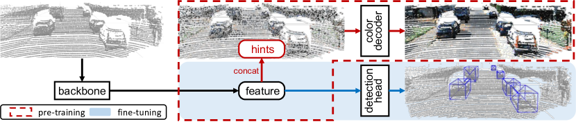
Figure 2: Architecture of GPC. The key insight is grounding the pre-training colorization process on the hints, allowing the model backbone to focus on learning semantically meaningful representations that indicate which subsets (i.e., segments) of points should be colored similarly to facilitate downstream 3D object detection.

Taking a point-based backbone $f_{\bm{\theta}}$ like PointNet++ (Qi et al., 2017b) as an example, the model takes $\bm{X}$ as input and outputs a feature matrix $\hat{\bm{Z}}\in\mathbb{R}^{D\times N}$, in which each column vector $\hat{{\bm{z}}}_{n}\in\mathbb{R}^{D}$ is meant to capture semantic cues for the corresponding point ${\bm{x}}_{n}$ to facilitate 3D object detection. One way to pre-train $f_{\bm{\theta}}$ using $(\bm{X},\bm{Y})$ is to add another point-based model $g_{\bm{\phi}}$ (seen as the projection head or color decoder) on top of $f_{\bm{\theta}}$, which takes $\hat{\bm{Z}}$ as input and output $\hat{\bm{Y}}$ of the same shape as $\bm{Y}$. In this way, $\hat{\bm{Y}}$ can be compared with $\bm{Y}$ to derive the loss, for example, the Frobenius norm. Putting things together, we come up with the following optimization problem,

$$\min_{\bm{\theta},\bm{\phi}}\sum_{(\bm{X},\bm{Y})\in\bm{D}_{\text{train}}}\|g_{\bm{\phi}}\circ f_{\bm{\theta}}(\bm{X})-\bm{Y}\|^{2}_{F}=\min_{\bm{\theta},\bm{\phi}}\sum_{(\bm{X},\bm{Y})\in\bm{D}_{\text{train}}}\sum_{n}\|\hat{\bm{y}}_{n}-\bm{y}_{n}\|^{2}_{2},$$ (1)

where $\bm{D}_{\text{train}}$ means the pre-training dataset and $\hat{\bm{y}}_{n}$ is the $n$-th column of $\hat{\bm{Y}}=g_{\bm{\phi}}\circ f_{\bm{\theta}}(\bm{X})$.

The inherent color variation.

At first glance, Eq. 1 should be fairly straightforward to optimize using standard optimizers like stochastic gradient descent (SGD). In our experiments, we however found a drastically slow drop in training error, which results from the inherent color variation. That is, given $\bm{X}$, there is a huge variation of $\bm{Y}$ in the collected data due to environmental factors (e.g., when the image is taken) or color options (e.g., instances of the same object can have different colors). This implies a huge entropy in the conditional distribution $P(\bm{Y}|\bm{X})$, i.e., a large $H(\bm{Y}|\bm{X})=\mathbb{E}[-\log(\bm{Y}|\bm{X})]$, indicating a small mutual information between $\bm{X}$ and $\bm{Y}$, i.e., a small $I(\bm{X};\bm{Y})=H(\bm{Y})-H(\bm{Y}|\bm{X})$. In other words, Eq. 1 may not provide sufficient information for $f_{\bm{\theta}}$ to learn.

Another way to look at this issue is the well-known bias-variance decomposition (Hastie et al., 2009; Bishop & Nasrabadi, 2006) in regression problems (suppose $\bm{Y}\in\mathbb{R}$), which contains a “noise” term,

$$\textbf{Noise: }\mathbb{E}_{\bm{Y},\bm{X}}\left[(\bm{Y}-\mathbb{E}_{\bm{Y}|\bm{X}}[\bm{Y}])^{2}\right].$$ (2)

When $P(\bm{Y}|\bm{X})$ has a high entropy, the noise term will be large, which explains the poor training error. Importantly, this noise term cannot be reduced solely by adopting a better model architecture. It can only be resolved by changing the data, or more specifically, how we leverage $(\bm{X},\bm{Y})$.

One intuitive way to reduce $H(\bm{Y}|\bm{X})$ is to manipulate $P(\bm{Y}|\bm{X})$, e.g., to carefully sub-sample data to reduce the variation. However, this would adversely reduce the amount of training data and also lead to a side effect of selection bias (Cawley & Talbot, 2010). In the extreme case, the pre-trained model may simply memorize the color of each distinct point cloud via the color decoder $g_{\bm{\phi}}$, preventing the backbone $f_{\bm{\theta}}$ from learning a useful embedding space for the downstream task.

Grounded colorization with hints.

To resolve these issues, we propose to reduce the variance in $P(\bm{Y}|\bm{X})$ by providing additional conditioning evidence $\bm{S}$. From the perspective of information theory (Cover, 1999), adding evidence into $P(\bm{Y}|\bm{X})$, i.e., $P(\bm{Y}|\bm{X},\bm{S})$, guarantees,

$$H(\bm{Y}|\bm{X})\geq H(\bm{Y}|\bm{X},\bm{S}),\quad\text{ and thus }\quad I((\bm{X},\bm{S});\bm{Y})\geq I(\bm{X};\bm{Y}),$$ (3)

unveiling more information for $f_{\bm{\theta}}$ to learn.

We realize this idea by proving ground-truth colors to a seed set of points in $\bm{X}$. Without loss of generality, we decompose $\bm{X}$ into two subsets $\bm{X}_{S}$ and $\bm{X}_{U}$ such that $\bm{X}=[\bm{X}_{S},\bm{X}_{U}]$. Likewise, we decompose $\bm{Y}$ into $\bm{Y}_{S}$ and $\bm{Y}_{U}$ such that $\bm{Y}=[\bm{Y}_{S},\bm{Y}_{U}]$. We then propose to inject $\bm{Y}_{S}$ as the conditioning evidence $\bm{S}$ into the colorization process. In other words, we directly provide the ground-truth colors to some of the points the model initially has to predict.

At first glance, this may controversially simplify the pre-training objective in Eq. 1. However, as the payback, we argue that this hint would help ground the colorization process on the inherent color variation, enabling the model to learn useful semantic cues for downstream 3D object detection. Concretely, to colorize a point cloud, the model needs to a) identify the segments that should possess similar colors and b) decide what colors to put on. With the hint that directly colors some of the points, the model can concentrate more on the first task, which aligns with the downstream task — to identify which subset of points to segment together.

Sketch of implementation.

We implement our idea by injecting $\bm{Y}_{S}$ as additional input to the color decoder $g_{\bm{\phi}}$. We achieve this by concatenating $\bm{Y}_{S}$ row-wise with the corresponding columns in $\hat{\bm{Z}}$, resulting in a $(D+3)$-dimensional input to $g_{\bm{\phi}}$. Let $\bm{O}_{U}$ denote an all-zero matrix with the same shape as $\bm{Y}_{U}$, we modify Eq. 1 as,

$$\min_{\bm{\theta},\bm{\phi}}\sum_{(\bm{X},\bm{Y})\in\bm{D}_{\text{train}}}\left\|g_{\bm{\phi}}\left(\left[\hat{\bm{Z}};[\bm{Y}_{S},\bm{O}_{U}]\right]\right)-[\bm{Y}_{S},\bm{Y}_{U}]\right\|^{2}_{F},\quad{s.t.}\quad\hat{\bm{Z}}=f_{\bm{\theta}}\left([\bm{X}_{S},\bm{X}_{U}]\right),$$ (4)

where “;” denotes row-wise concatenation. Importantly, Eq. 4 only provides the hint $\bm{Y}_{S}$ to the color decoder $g_{\bm{\phi}}$, leaving the input and output formats of the backbone model $f_{\bm{\theta}}$ intact. We name our approach Grounded Point Colorization (GPC).

GPC could mitigate selection bias.

Please see Appendix S1 for a discussion.

3.2 Details of Grounded Point Colorization (GPC)

Model architecture.

For the backbone $f_{\bm{\theta}}$, we use the model architectures defined in existing 3D object detectors. We specifically focus on detectors that use point-based feature extractors, such as PointRCNN (Shi et al., 2019) and IA-SSD (Zhang et al., 2022b). The output of $f_{\bm{\theta}}$ is a set of point-wise features denoted by $\hat{\bm{Z}}$. For the color decoder $g_{\bm{\phi}}$ that predicts the color of each input point, without loss of generality, we use a PointNet++ (Qi et al., 2017b).

Color regression vs. color classification.

In Sec. 3.1, we frame colorization as a regression problem. However, regressing the RGB pixel values is sensitive to potential outlier pixels. In our implementation, we instead consider a classification problem by quantizing real RGB values into discrete bins. We apply the K-means algorithm over pixels of the pre-training images to cluster them into $K$ classes. The label of each LiDAR point ${\bm{x}}_{n}$ then becomes $y_{n}\in\{1,\cdots,K\}$. Fig. 3 shows the images with color quantization; each pixel is colored by the assigned cluster center. It is hard to distinguish the images with $K=128$ bins from the original image by human eyes.

We accordingly modify the color decoder $g_{\bm{\phi}}$. In the input, we concatenate a $K$-dimensional vector to the feature $\hat{{\bm{z}}}_{n}\in\mathbb{R}^{D}$ of each LiDAR point ${\bm{x}}_{n}$, resulting in a $(D+K)$-dimension input to $g_{\bm{\phi}}$. For seed points where we inject ground-truth colors, the $K$-dimensional vector is one-hot, whose $y_{n}$-th element is one and zero elsewhere. For other LiDAR points, the $K$-dimensional vector is a zero vector. In the output, $g_{\bm{\phi}}$ generates a $K$-dimensional logit vector $\hat{\bm{\eta}}_{n}\in\mathbb{R}^{K}$ for each input point ${\bm{x}}_{n}$. The predicted color class $\hat{y}_{n}$ can be obtained by $\operatorname{arg\,max}_{c\in\{1,\cdots,K\}}\hat{\eta}_{n}[c]$.

Figure 3: Color quantization. We apply the K-Means algorithm to cluster RGB pixel values into discrete bins. The resulting image with $128$ bins is hardly distinguishable from the original image by human eyes.

Pre-training objective.

The cross-entropy loss is the standard loss for classification. However, in driving scenes, most of the LiDAR points are on the ground, leading to an imbalanced distribution across color classes. We thus apply the Balanced Softmax (Ren et al., 2020) to re-weight each class,

$$\ell({\bm{x}}_{n},y_{n})=-\log\left(\frac{\alpha_{y_{n}}\times\mathrm{e}^{\hat{\eta}_{n}[y_{n}]}}{\sum_{c=1}^{K}\alpha_{c}\times\mathrm{e}^{\hat{\eta}_{n}[c]}}\right),$$ (5)

where $\alpha_{c}$ is the balance factor of class $c$. In the original paper (Ren et al., 2020), $\alpha_{c}$ is proportional to the number of training examples of class $c$. Here, we set $\alpha_{c}$ per mini-batch, proportional to the number of LiDAR points with class label $c$. A small $\epsilon$ is added to $\alpha_{c}$ for stability since an image may not contain all colors at once.

Optimization.

In the pre-training stage, we train $f_{\bm{\theta}}$ and $g_{\bm{\phi}}$ end-to-end without human supervision. In the fine-tuning stage with labeled 3D object detection data, $g_{\bm{\phi}}$ is disregarded; the pre-trained $f_{\bm{\theta}}$ is fine-tuned end-to-end with other components in the 3D object detector.

All pieces together.

We propose a novel self-supervised learning algorithm GPC, which leverages colors to pre-train LiDAR-based 3D detectors. The model includes a backbone $f_{\bm{\theta}}$ and a color decoder $g_{\bm{\phi}}$; $f_{\bm{\theta}}$ learns to generate embeddings to segment LiDAR points while $g_{\bm{\phi}}$ learns to colorize LiDAR points. To mitigate the inherent color variation, GPC injects hints into $g_{\bm{\phi}}$. To overcome the potential outlier pixels, GPC quantizes colors into class labels and treats colorization as a classification problem. Fig. 1 shows our main insight and Fig. 2 shows the architecture.

Extension to voxel-based features.

As mentioned in Sec. 2, another branch of LiDAR-based detectors encode LiDAR points into a voxel-based, bird’s-eye view (BEV) feature representation. GPC can still be beneficial to these LiDAR-based detectors by offering better input data — augmenting the LiDAR point coordinates with the output features by the pre-trained point-based backbone $f_{\bm{\theta}}$. We investigate this idea in Sec. 4.2 and demonstrate promising results.

4 Experiments

4.1 Setup

Datasets.

We use two commonly used datasets in autonomous driving: KITTI (Geiger et al., 2012) and Waymo Open Dataset (Sun et al., 2020). KITTI contains $7,481$ annotated samples, with $3,712$ for training and $3,769$ for validation. Waymo dataset is much larger, with $158,081$ frames in $798$ scenes for training and $40,077$ frames in $202$ scenes for validation. We pre-train on each dataset with all training examples without using any labels in the pre-training. We then fine-tune on different amounts of KITTI data, $5\%$, $10\%$, $20\%$, $50\%$, and $100\%$, with 3D annotations to investigate data-efficient learning. We adopt standard evaluation on KITTI validation set. Experiments of KITTI $\rightarrow$ KITTI show the in-domain performance. Waymo $\rightarrow$ KITTI provides the scalability and transfer ability of the algorithm, which is the general interest in SSL.

3D Detectors.

As mentioned in Sec. 3, we focus on learning effective point representation with PointRCNN and IA-SSD. We see consistent improvement on both (Sec. 4.2). Additionally, we extend GPC to Voxel-based detectors as discussed in Sec. 4.2.

Implementation.

We sample images from the training set ($3$k and $10$k for KITTI and Waymo respectively) and $1$k pixels for each image to learn the quantization. KMeans algorithm is adopted to cluster the colors into $128$ discrete labels which are used for seeds and ground truths. The color labels in one hot concatenated with the features from the backbone are masked out $80\%$ of colors (i.e., assigned to zeros). During the pre-training, we colorjitter the image with a probability of 0.5. For 3D point augmentation, we follow the standard procedure, random flipping along the X-axis, random rotation ($[-4/\pi,4/\pi]$), random scaling ($[0.95,1.05]$), random point sampling ($N=16384$ with range$=40$), and random point shuffling. We pre-train the model for 80 and 12 epochs on KITTI and Waymo respectively with batch size 16 and 32. We fine-tune on subsets of KITTI for 80 epochs with a batch size of 16 and the same 3D point augmentation above. The AdamW optimizer (Loshchilov & Hutter, 2017) and Cosine learning rate scheduler(Loshchilov & Hutter, 2016) are adopted in both stages which the maximum learning rate is $0.001$ and $0.0004$ respectively.

Table 1: Pre-trained on KITTI and fine-tuned on subsets of KITTI. GPC is consistently better than scratch and PointContrast (Xie et al., 2020) especially when labeled data are extremely sparse.

Sub.	Method	Detector	Car			Pedestrian			Cyclist			Overall
			easy	mod.	hard	easy	mod.	hard	easy	mod.	hard	easy	mod.	hard
	scratch	PointRCNN	66.8	51.6	45.0	61.5	55.4	48.3	81.4	58.6	54.5	69.9	55.2	49.3
	PointContrast	PointRCNN	58.2	46.7	40.1	52.5	47.5	42.0	73.1	49.7	46.6	61.2	47.9	42.9
	GPC (Ours)	PointRCNN	81.2	65.1	57.7	63.7	57.4	50.3	88.2	65.7	61.4	77.7	62.7	56.7
2-15	scratch	IA-SSD	73.7	61.6	55.3	41.2	32.0	29.2	75.1	54.2	51.1	63.3	49.3	45.2
$5\%$	GPC (Ours)	IA-SSD	81.3	66.6	59.7	49.2	40.5	36.7	77.3	54.7	51.2	69.3	53.9	49.2
	scratch	PointRCNN	87.6	74.2	71.1	68.2	60.3	52.9	93.0	71.8	67.2	82.9	68.8	63.7
	PointContrast	PointRCNN	88.4	73.9	70.7	71.0	63.6	56.3	86.8	69.1	64.1	82.1	68.9	63.7
	GPC (Ours)	PointRCNN	88.7	76.0	72.0	70.6	63.0	55.8	92.6	73.0	68.1	84.0	70.7	65.3
2-15	scratch	IA-SSD	86.1	74.0	70.6	52.2	45.6	40.1	84.5	64.0	59.8	74.3	61.2	56.8
$20\%$	GPC (Ours)	IA-SSD	87.6	76.4	71.5	54.1	47.3	42.0	86.2	69.5	64.9	76.0	64.4	59.5
	scratch	PointRCNN	89.7	77.4	74.9	68.9	61.3	54.2	88.4	69.2	64.4	82.3	69.3	64.5
	PointContrast	PointRCNN	89.1	77.3	74.8	69.2	62.0	55.1	90.4	70.8	66.5	82.9	70.0	65.4
	GPC (Ours)	PointRCNN	89.3	77.5	75.0	68.4	61.4	54.7	92.1	72.1	67.6	83.3	70.3	65.8
2-15	scratch	IA-SSD	88.6	77.6	74.2	61.8	55.0	49.0	89.9	70.0	65.6	80.1	67.5	63.0
$50\%$	GPC (Ours)	IA-SSD	89.3	80.1	76.9	62.5	55.4	49.6	88.8	73.7	69.2	80.2	69.7	65.2
	scratch	PointRCNN	90.8	79.9	77.7	68.1	61.1	54.2	87.3	68.1	63.7	82.0	69.7	65.2
	PointContrast	PointRCNN	91.1	80.0	77.5	66.9	61.1	54.7	91.3	70.7	66.4	83.1	70.6	66.2
	GPC (Ours)	PointRCNN	90.8	79.6	77.4	68.5	61.3	54.7	92.3	71.8	67.1	83.9	70.9	66.4
2-15	scratch	IA-SSD	89.3	80.5	77.4	60.1	52.9	46.7	87.8	69.7	65.2	79.1	67.7	63.1
$100\%$	GPC (Ours)	IA-SSD	89.3	82.5	79.6	60.2	54.9	49.0	88.6	71.3	67.2	79.3	69.6	65.3

4.2 Results

Results on KITTI $\rightarrow$ KITTI.

We first study in-domain data-efficient learning with different amounts of labeled data available. Our results outperform random initialization (scratch) by a large margin, particularly when dealing with limited human-annotated data, as shown in Sec. 4.1. For instance, with PointRCNN, on $5\%$ KITTI, we improve +$7.5\%$ on overall moderate AP ($55.2$ to $62.7$). Remarkably, even with just $20\%$ KITTI, we already surpass the performance achieved by training on the entire dataset from scratch, reaching a performance of $70.7$. This highlights the essential benefit of GPC in data-efficient learning, especially when acquiring 3D annotations is expensive. Moreover, even when fine-tuning on the entire $100\%$ of the data, we still achieve a notable gain, improving from $69.7$ to $70.9$ (+$1.2$).

To provide a robust comparison, we re-implement a recent method, PointContrast (Xie et al., 2020), as a stronger baseline. GPC performs better across all subsets of data. Notice that PointContrast struggles when annotations are extremely scarce, as seen on $5\%$ subset where it underperforms the baseline ($47.9$ vs.$55.2$).

Table 2: Pre-trained on Waymo and fine-tuned on subsets of KITTI. We compare with DepthContrast (Zhang et al., 2021) and ProposalContrast (Yin et al., 2022). ^†directly taken from Yin et al. (2022).

Sub.	Method	Detector	Car			Pedestrian			Cyclist			Overall
			easy	mod.	hard	easy	mod.	hard	easy	mod.	hard	easy	mod.	hard
	scratch	PointRCNN	66.8	51.6	45.0	61.5	55.4	48.3	81.4	58.6	54.5	69.9	55.2	49.3
	GPC (Ours)	PointRCNN	83.9	67.8	62.5	64.6	58.1	51.5	88.3	65.9	61.6	78.9	63.9	58.5
2-15	scratch	IA-SSD	73.7	61.6	55.3	41.2	32.0	29.2	75.1	54.2	51.1	63.3	49.3	45.2
$5\%$	GPC (Ours)	IA-SSD	81.5	67.4	60.1	47.2	39.5	34.5	81.2	61.4	57.4	70.0	56.1	50.7
	scratch†	PointRCNN	88.6	75.2	72.5	55.5	48.9	42.2	85.4	66.4	71.7		63.5
	ProposalContrast†	PointRCNN	88.5	77.0	72.6	58.7	51.9	45.0	90.3	69.7	65.1		66.2
	GPC (Ours)	PointRCNN	90.9	76.6	73.5	70.5	62.8	55.5	89.9	71.0	66.6	83.8	70.1	65.2
2-15	scratch	IA-SSD	86.1	74.0	70.6	52.2	45.6	40.1	84.5	64.0	59.8	74.3	61.2	56.8
$20\%$	GPC (Ours)	IA-SSD	88.1	76.8	71.9	58.2	50.9	44.6	86.1	66.2	62.1	77.4	64.6	59.5
	scratch†	PointRCNN	89.1	77.9	75.4	61.8	54.6	47.9	86.3	67.8	63.3		66.7
	ProposalContrast†	PointRCNN	89.3	80.0	77.4	62.2	54.5	46.5	92.3	73.3	68.5		69.2
	GPC (Ours)	PointRCNN	89.5	79.2	77.0	69.3	61.8	54.6	89.1	71.3	66.4	82.7	70.7	66.0
2-15	scratch	IA-SSD	88.6	77.6	74.2	61.8	55.0	49.0	89.9	70.0	65.6	80.1	67.5	63.0
$50\%$	GPC (Ours)	IA-SSD	88.4	79.8	76.4	63.4	56.2	49.6	88.3	70.5	66.0	80.1	68.9	64.0
	scratch†	PointRCNN	90.0	80.6	78.0	62.6	55.7	48.7	89.9	72.1	67.5		69.5
	DepthContrast†	PointRCNN	89.4	80.3	77.9	65.6	57.6	51.0	90.5	72.8	68.2		70.3
	ProposalContrast†	PointRCNN	89.5	80.2	78.0	66.2	58.8	52.0	91.3	73.1	68.5		70.7
	GPC (Ours)	PointRCNN	89.1	79.5	77.2	67.9	61.5	55.0	89.1	71.0	67.0	82.0	70.7	66.4
2-15	scratch	IA-SSD	89.3	80.5	77.4	60.1	52.9	46.7	87.8	69.7	65.2	79.1	67.7	63.1
$100\%$	GPC (Ours)	IA-SSD	90.7	82.4	79.5	60.7	55.0	49.5	86.5	70.5	67.1	79.3	69.3	65.4

Table 3: Comparison with methods using images. PPKT (Liu et al., 2021), SLidR (Sautier et al., 2022), and TriCC (Pang et al., 2023) pre-train on NuScenes (Caesar et al., 2020) with UNet (Choy et al., 2019). The results are shown in moderate AP. ^†directly taken from Pang et al. (2023).

Method	Arch	Pre. Dataset	5%	10%	20%
scratch†	UNet + PointRCNN	-	56.6	58.8	63.7
PPKT†	UNet + PointRCNN	NuScenes	59.6  (+3.0)	63.7  (+4.9)	64.8  (+1.1)
SLidR†	UNet + PointRCNN	NuScenes	58.8  (+2.2)	63.5  (+4.7)	63.8  (+0.1)
TriCC†	UNet + PointRCNN	NuScenes	61.3  (+4.7)	64.6  (+5.8)	65.9  (+2.2)
scrach	PointRCNN	-	55.2	65.2	68.8
GPC (Ours)	PointRCNN	KITTI	62.7  (+7.5)	66.4  (+1.2)	70.7  (+1.9)
GPC (Ours)	PointRCNN	Waymo	63.9  (+8.7)	67.0  (+1.8)	70.1  (+1.3)

Table 4: Pre-train and fine-tune on Waymo. Performance of LEVEL 2 is reported.

Sub.	Method	Detector	Vehicle		Pedestrian		Cyclist		Overall
			AP	APH	AP	APH	AP	APH	AP	APH
	scratch	IA-SSD	45.55	44.60	32.88	16.75	43.07	29.06	40.50	30.14
$1\%$	GPC (Ours)	IA-SSD	48.25	47.53	37.09	23.90	43.42	35.30	42.92	35.58

Table 5: GPC on SECOND (Yan et al., 2018). The result shows that the point representation by GPC can be a good plug-and-play in addition to the point coordinate (i.e. xyz) for voxel-based detectors.

Sub.	Method	Pre. on	Car			Pedestrian			Cyclist			Overall
			easy	mod.	hard	easy	mod.	hard	easy	mod.	hard	easy	mod.	hard
	scratch	-	64.9	52.7	45.3	44.3	39.9	35.0	71.0	50.4	47.1	60.1	47.7	42.5
$5\%$	GPC (Ours)	Waymo	69.5	57.1	50.5	50.1	43.4	38.7	74.2	53.8	49.9	64.6	51.4	46.4
	scratch	-	83.9	71.7	67.4	54.7	48.2	42.8	74.3	58.0	54.6	71.0	59.3	54.9
$20\%$	GPC (Ours)	Waymo	85.1	72.3	67.8	56.6	48.7	43.3	75.4	59.6	55.8	72.4	60.2	55.6
	scratch	-	88.1	76.2	73.2	59.7	52.4	46.0	83.9	63.0	59.4	77.2	63.8	59.5
$50\%$	GPC (Ours)	Waymo	88.0	76.3	73.5	60.7	53.3	47.0	85.5	67.5	63.4	78.1	65.7	61.3
	scratch	-	88.1	78.3	73.7	62.0	54.4	47.6	81.1	62.4	58.7	77.1	65.0	60.0
$100\%$	GPC (Ours)	Waymo	90.9	79.1	76.2	65.2	56.9	50.0	82.5	64.5	60.6	79.5	66.8	62.3

Table 6: Loss ablation for colorization. We explore two regression losses Mean Squared Error (MSE), SmoothL1 (SL1) and two classification losses CrossEntropy (CE), modified Balanced Softmax (BS). The results are on KITTI $\rightarrow 5\%$ KITTI.

Loss	Type	Car			Pedestrian			Cyclist			Overall
		easy	mod.	hard	easy	mod.	hard	easy	mod.	hard	easy	mod.	hard
scratch	-	66.8	51.6	45.0	61.5	55.4	48.3	81.4	58.6	54.5	69.9	55.2	49.3
MSE	reg	72.4	59.8	52.9	64.2	56.2	49.2	86.2	64.2	60.2	74.2	60.1	54.1
SL1	reg	76.8	62.9	56.0	63.2	55.6	49.2	84.1	63.3	58.9	74.7	60.6	54.7
CE	cls	78.4	64.5	58.5	60.7	54.1	47.6	85.5	61.5	57.6	74.9	60.0	54.6
BS	cls	81.2	65.1	57.7	63.7	57.4	50.3	88.2	65.7	61.4	77.7	62.7	56.5

Results on Waymo $\rightarrow$ KITTI.

We investigate the transfer learning ability on GPC as it’s the general interest in SSL. We pre-train on Waymo (20$\times$ larger than KITTI) and fine-tune on subsets of KITTI. In  Sec. 4.2, our method shows consistent improvement upon scratch baseline. The overall moderate AP improves $55.2\rightarrow 63.9$ on $5\%$ KITTI. On $20\%$, it improves $63.5\rightarrow 70.1$ which is again already better than $100\%$ from scratch ($69.5$). We compare to the current SOTA, ProposalContrast (Yin et al., 2022), and GPC outperforms on $20\%$ ($66.2$ vs.$70.1$) and $50\%$ ($69.2$ vs.$70.7$).

Learning with Images.

We’ve noticed recent efforts in self-supervised learning using images (see Sec. 2), where most approaches use separate feature extractors for LiDAR and images to establish correspondences for contrastive learning. In contrast, our method, GPC, directly utilizes colors within a single trainable architecture. We strive to incorporate numerous baselines for comparison, but achieving a fair comparison is challenging due to differences in data processing, model architecture, and training details. Therefore, we consider the baselines as references that demonstrate our approach’s potential, rather than claiming state-of-the-art status.

In Tab. 3, we compare to PPKT (Liu et al., 2021), SLidR (Sautier et al., 2022) and TriCC (Pang et al., 2023) with moderate AP reported in Pang et al. (2023). Notably, on $5\%$ KITTI, we outperform the baselines with substantial gains of +$7.5$ and +$8.7$, which are significantly higher than their improvements (less than +4.7).

Results on Waymo $\rightarrow$ Waymo.

We evaluate on $1\%$ Waymo with its standard metric AP and APH. The result in Tab. 4 shows that GPC improve +$2.4\%$ on AP and +$4.4\%$ on APH.

Extension to Voxel-Based Detector.

We further extend the applicability of GPC to SECOND (Yan et al., 2018), a widely-used voxel-based backbone, by concatenating our pre-trained per-point feature with the raw input (i.e., the LiDAR point coordinate) to SECOND. The results in Tab. 5 show that GPC consistently improve upon the scratch baseline, suggesting the effectiveness of our learned features. We hypothesize GPC can also be a good plug-and-play for algorithms pooling with point features in the later stage (Shi et al., 2020a). Please see more details in the Appendix S5.

4.3 Ablation Study

Colorization with regression or classification?

In Tab. 6, we explore four losses for colorization. There is nearly no performance difference in using MSE, SL1, and CE, but BS outperforms other losses by a clear margin. We hypothesize that it prevents the learning biased toward the ground (major pixels) and force the model to learn better on foreground objects that have much fewer pixels which facilitates the downstream 3D detection as well.

Hint mechanism.

It is the key design to overcome the inherent color variation (see Sec. 3). In Tab. 9, we directly regress RGB values (row 2 and 3) without hints and color decoders. The performance is still better than scratch but limited. We hypothesize that the naive regression is sensitive to pixel values and can’t learn well if there exists a large color variation. On the other hand, the hint resolves the above issue and performs much better (row 4, $62.7$ and row 5, $63.9$). In Tab. 9, we ablate different levels of hint and find out providing only $20\%$ as seeds is the best ($61.9$), suggesting the task to learn can’t be too easy (i.e., providing too many hints). On the other hand, providing no hints falls into the issue of color variation again, deviating from learning a good representation ($0\%$, 44.1 worse than scratch, $55.2$).

Repeated experiments.

To address potential performance fluctuations with different data sampled for fine-tuning, we repeat the $5\%$ fine-tuning experiment for another five rounds, each with a distinctly sampled subset, as shown in Appendix S3. The results show the consistency and promise of GPC.

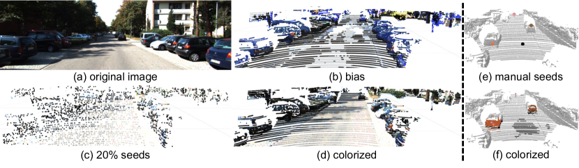
Figure 4: Qualitative results of colorization. (left) We use trained GPC to infer on validation LiDAR (b) without any seeds and with (c) resulting in (d). The model learned the bias about the driving scene: the ground is gray and black, trees are green, and tail lights are red, but it predicts the average color on all cars because they can be variant. On the other hand, it correctly colorizes the point cloud if some hints are provided. We hypothesize such an ability to know where to pass the color is essential for downstream 3D detection. (right) (e) We further manipulate the seeds by hand. (f) GPC successfully colorize the regions with given colors in (e).

Table 7: Seed ratios. seed easy mod. hard 100% 51.7 38.7 33.8 80% 66.4 50.5 44.9 60% 74.8 58.8 52.2 40% 75.1 59.7 53.4 20% 77.1 61.9 56.2 0% 57.9 44.1 38.4 scratch 69.9 55.2 49.3 Table 8: Hint mechanism. Hint Pre. Dataset easy mod. hard scratch - 69.9 55.2 49.3 KITTI 75.1 59.4 53.3 Waymo 74.9 60.4 54.5 ✓ KITTI 77.7 62.7 56.5 ✓ Waymo 78.9 63.9 58.5 Table 9: Number of epochs pertaining on Waymo. epochs easy mod. hard 1 75.8 60.7 54.4 4 76.4 61.6 55.9 8 78.3 63.1 58.4 12 78.9 63.9 58.5

4.4 Qualitative Results

We validate GPC by visualization as shown in Fig. 4 (left). Impressively the model can learn common sense about colors in the driving scene in (b), even red tail lights on cars. We further play with manual seeds to manipulate the object colors (Fig. 4 (right)) and it more or less recognizes which points should have the same color and stops passing to the ground.

4.5 Discussion

We reiterate that we explore a new perspective to pre-train LiDAR-based detectors (see Sec. 2). GPC outperforms or performs on par with the mainstream contrastive learning-based methods, such as the state-of-the-art method ProposalContrast (Yin et al., 2022), suggesting our new perspective as a promising direction to explore further.

5 Conclusion

Color images collected along with LiDAR data offer valuable semantic cues about objects. We leverage this insight to frame pre-training LiDAR-based 3D object detectors as a supervised colorization problem, a novel perspective drastically different from the mainstream contrastive learning-based approaches. Our proposed approach, Grounded Point Colorization (GPC), effectively addresses the inherent variation in the ground-truth colors, enabling the model backbone to learn to identify LiDAR points belonging to the same objects. As a result, GPC could notably facilitate downstream 3D object detection, especially under label-scarce settings, as evidenced by extensive experiments on benchmark datasets. We hope our work can vitalize the community with a new perspective.

Acknowledgment

This research is supported in part by grants from the National Science Foundation (IIS-2107077, OAC-2118240, OAC-2112606, IIS-2107161, III-1526012, and IIS-1149882), NVIDIA research, and Cisco Research. We are thankful for the generous support of the computational resources by the Ohio Supercomputer Center. We also thank Mengdi Fan for her valuable assistance in creating the outstanding figures for this work.

Pre-training LiDAR-based 3D Object Detectors through Colorization

In this supplementary material, we provide more details and experiment results in addition to the main paper:

• Appendix S1: discusses how GPC could mitigate selection bias.

• Appendix S2: provides more evidence to show the effectiveness of GPC.

• Appendix S3: repeats the experiments to show consistent performance.

• Appendix S4: explores another usage of color.

• Appendix S5: extends GPC to Voxel-Based backbone

Appendix S1 Grounded Point Colorization Could Mitigate Selection Bias

Another advantage of injecting hints into the colorization process is its ability to overcome selection bias Cawley & Talbot (2010) — the bias that only a few variations of $\bm{Y}$ conditioned on $\bm{X}$ are collected in the dataset. According to Clark et al. (2019) and Cadene et al. (2019), one effective approach to prevent the model from learning the bias is to proactively augment the bias to the “output” of the model during the training phase. The augmentation, by default, will reduce the loss on the training example that contains bias, allowing the model to focus on hard examples in the training set. We argue that our model design and objective function Eq. 4 share similar concepts with Clark et al. (2019) and Cadene et al. (2019).

Another way to mitigate bias in $\bm{Y}$ is to perform data augmentation, e.g., by color jittering. We note that this is not applicable through Eq. 1 as it will adversely increase the entropy $H(\bm{Y}|\bm{X})$, but is applicable through Eq. 4 via grounded colorization.

Appendix S2 Effectiveness of GPC

In the main paper, we show the superior performance of our proposed pre-training method, Grounded Point Colorization (GPC) (Sec. 4.2). With our pre-trained backbone, it outperforms random initialization as well as existing methods on fine-tuning with different amounts of labeled data (i.e.$5\%$, $20\%$, $50\%$, and $100\%$) of KITTI (Geiger et al., 2012). Significantly, fine-tuning on only $20\%$ with GPC is already better than training $100\%$ from scratch. Besides, GPC demonstrates the ability of transfer learning by pre-training on Waymo (Sun et al., 2020) in Sec. 4.2. Not to mention, GPC is fairly simpler than existing methods which require road planes for better region sampling, temporal information for pair construction to contrast, or additional feature extractors for different modalities (Sec. 2). Most importantly, We successfully explore a new perspective of the pre-training methods on LiDAR-based 3D detectors besides contrastive learning-based algorithms.

In this supplementary, we further provide the training curve besides the above evidence. Fig. S1 shows the evaluation on KITTI validation set and loss on the training set during the fine-tuning on $5\%$ KITTI. With GPC, the overall moderate AP raises faster than the scratch baseline and keeps the gain till the end. It already performs better at $55^{\text{th}}$ epoch than the final performance of scratch baseline, which is more than $30\%$ better in terms of efficiency. The training loss with GPC is also below the curve of the scratch baseline.

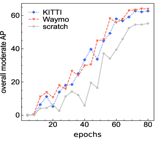
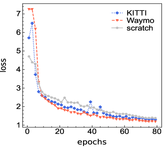
Figure S1: Training curve on 5% KITTI. (left) is the performance ($\uparrow$) on KITTI validation set and (right) is the loss ($\downarrow$) on the training set during the fine-tuning. It shows the effectiveness and efficiency of GPC compared to training from scratch.

With the above evidence and the extensive experiments in the main paper, we explain that GPC is a simple yet effective self-supervised learning algorithm for pre-training LiDAR-based 3D object detectors without human-labeled data.

Appendix S3 Repeated Experiments

To address potential performance fluctuations with different data sampled for fine-tuning, we repeat the $5\%$ fine-tuning experiment for another five rounds, each with a distinctly sampled subset. The results are summarized in Tab. S1, in which we compare the baseline of training from scratch (with $5\%$ KITTI data), pre-training with full KITTI (cf. Tab. 9 in the main paper), and pre-training with Waymo (cf. Sec. 4.2 in the main paper). Pre-training with our GPC consistently outperforms the baseline. Notably, the standard deviation among the five rounds is largely reduced with pre-training. For instance, the standard deviation of the overall moderate AP is 2.7 with the scratch baseline, which is reduced to 0.6 with GPC. This significant reduction in standard deviation underscores the consistency and promise of our proposed method.

Table S1: Repeat experiments. We re-sample 5 different subsets of 5% KITTI and repeat the experiments. The standard deviation of overall moderate AP on the scratch baseline is 2.7, but it’s only 0.6 on GPC. It implies that our improvement is promising and constant, regardless of the performance on the baseline.

Exp.	Pre.	Car			Pedestrian			Cyclist			Overall
		easy	mod.	hard	easy	mod.	hard	easy	mod.	hard	easy	mod.	hard
	scratch	51.3	41.9	36.2	56.9	51.4	45.0	74.5	53.7	50.0	60.9	49.0	43.7
	KITTI	79.2	65.5	59.1	62.7	55.5	48.4	87.9	65.0	61.0	76.6	62.0	56.1
1	Waymo	83.8	68.4	63.1	65.6	58.7	51.4	87.1	65.9	61.4	78.8	64.3	58.7
	scratch	44.0	36.5	31.6	54.6	48.8	43.0	70.9	48.7	45.5	56.5	44.7	40.1
	KITTI	81.1	65.0	58.8	60.3	53.7	47.4	86.8	63.4	59.4	76.1	60.7	55.2
2	Waymo	82.2	67.6	62.4	64.2	57.3	50.9	87.0	65.3	61.5	77.8	63.4	58.3
	scratch	63.0	49.1	42.1	57.6	51.3	44.8	80.6	58.0	53.8	67.1	52.8	46.9
	KITTI	78.3	64.0	56.9	61.4	54.4	47.3	86.5	62.6	58.5	75.4	60.3	54.2
3	Waymo	80.2	64.5	59.5	65.9	57.6	50.7	86.4	66.1	61.8	77.5	62.7	57.3
	scratch	59.5	46.3	39.2	52.9	47.9	42.0	72.4	51.1	47.7	61.6	48.4	43.0
	KITTI	82.5	67.4	60.1	64.9	57.0	49.7	87.6	65.4	61.1	78.3	63.3	57.0
4	Waymo	85.1	68.4	63.1	63.5	56.7	50.0	87.4	66.3	62.1	78.7	63.8	58.4
	scratch	52.6	42.8	36.8	51.8	47.3	42.0	71.2	50.0	46.6	58.5	46.7	41.8
	KITTI	81.1	65.2	58.9	60.7	53.8	46.9	89.8	65.7	61.7	77.2	61.6	55.9
5	Waymo	84.5	68.4	64.9	65.0	57.3	51.3	87.0	66.4	62.5	78.8	64.0	59.6

Appendix S4 Correct Usage of Color

GPC uses color to provide semantic cues to pre-train LiDAR-based 3D detectors (c.f. Sec. 3 in the main paper). With extensive experiments (c.f. Sec. 4.2 and Sec. 4.3), we show that the hint mechanism is the key to learning good point representation. Naive regression of color without hints can hurt performance. In this supplementary, we further explore a possibility: directly concatenating the input coordinate (i.e.xyz) with pixel values (i.e.RGB) to form a 6-dimension input vector. As shown in Tab. S2, the performance is even worse than plain scratch. It implies that the additional color information on the input isn’t necessary to obtain the richer representation. On the other hand, using it with GPC in the pre-training stage shows significant improvement. We argue that how to leverage color information correctly is not trivial. Also, notice that color is no longer needed during fine-tuning.

Table S2: Comparison of usages of color. Directly concatenating the color (i.e.RGB) and the coordinate (i.e.xyz) performs worse than plan scratch on all subsets. In contrast, GPC utilizing the color as semantic cues in the pre-training brings significant improvement.

Sub.	Method	Car			Pedestrian			Cyclist			Overall
		easy	mod.	hard	easy	mod.	hard	easy	mod.	hard	easy	mod.	hard
	scratch	66.8	51.6	45.0	61.5	55.4	48.3	81.4	58.6	54.5	69.9	55.2	49.3
	w/ color	57.5	46.3	38.9	50.8	46.6	41.1	72.9	54.1	50.5	60.4	49.0	43.5
$5\%$	GPC	81.2	65.1	57.7	63.7	57.4	50.3	88.2	65.7	61.4	77.7	62.7	56.7
	scratch	87.6	74.2	71.1	68.2	60.3	52.9	93.0	71.8	67.2	82.9	68.8	63.7
	w/ color	87.4	73.6	70.2	60.4	54.8	48.6	90.0	69.9	65.3	79.2	66.1	61.4
$20\%$	GPC	88.7	76.0	72.0	70.6	63.0	55.8	92.6	73.0	68.1	84.0	70.7	65.3
	scratch	89.7	77.4	74.9	68.9	61.3	54.2	88.4	69.2	64.4	82.3	69.3	64.5
	w/ color	88.8	77.3	74.7	65.5	59.3	53.2	92.6	71.0	67.4	82.3	69.2	65.1
$50\%$	GPC	89.3	77.5	75.0	68.4	61.4	54.7	92.1	72.1	67.6	83.3	70.3	65.8
	scratch	90.8	79.9	77.7	68.1	61.1	54.2	87.3	68.1	63.7	82.0	69.7	65.2
	w/ color	90.8	80.0	77.5	63.2	57.0	51.4	89.5	69.7	65.1	81.2	68.9	64.7
$100\%$	GPC	90.8	79.6	77.4	68.5	61.3	54.7	92.3	71.8	67.1	83.9	70.9	66.4

Appendix S5 Extension to Voxel-Based Backbone

In this work, we mainly focus on pre-training PointNet++ (Qi et al., 2017b) while there exist other types of backbones such as PointPillars (Lang et al., 2019) or VoxelNet (Zhou & Tuzel, 2018; Yan et al., 2018). While it’s not our primary focus, we hypothesize that GPC can be modified to facilitate those architectures. For example, it can still learn to predict the color for each point within the unit (i.e.pillar or voxel) for better point-wise representation or the average color of each unit for better unit-wise representation.

In this supplementary, we explore the first idea mentioned above on SECOND (Yan et al., 2018). More specifically, instead of just using the coordinate of points in each voxel, we concatenate xyz with the feature from the PointNet++ backbone pre-trained by GPC (mathematically $\bm{X}^{\prime}=[\;\bm{X}\;|\;f_{\bm{\theta}}(\bm{X})\;]\in\mathbb{R}^{(3+D)\times N}$). SECOND is randomly initialized and no projection layers are added. PointNet++ backbone is frozen during the fine-tuning. All the other training details are standard without hard tuning, including data augmentation, training scheduler, optimizer, etc.

The result is shown in Tab. S3. Impressively, even with this approach, GPC still brings significant improvement upon the scratch baseline. On $5\%$ KITTI, it improves from $47.7$ to $52.6$ on overall moderate AP, which is a gain of $+4.9$. On $50\%$ KITTI, the performance of pre-training on Waymo ($65.7$) is already better than training with $100\%$ from scratch ($65.0$). Even on $100\%$ KITTI, GPC still brings more than $+1.5$ gain upon scratch baseline. It demonstrates the effectiveness of our learned point representation and opens the great potential of our proposed method.

Furthermore, some recent works (Shi et al., 2020a) show that using point-wise features for pooling in the latter stage can improve the performance of 3D detection. We hypothesize GPC can be plug-and-play for those algorithms.

Table S3: Approach with GPC on SECOND (Yan et al., 2018). The result shows that the point representation by GPC can be a good plug-and-play in addition to the point coordinate (i.e.xyz) for better 3D detection.

Sub.	Method	Pre. on	Car			Pedestrian			Cyclist			Overall
			easy	mod.	hard	easy	mod.	hard	easy	mod.	hard	easy	mod.	hard
	scratch	-	64.9	52.7	45.3	44.3	39.9	35.0	71.0	50.4	47.1	60.1	47.7	42.5
	GPC (Ours)	KITTI	74.9	60.8	54.1	46.8	41.9	37.3	74.2	55.0	51.5	65.3	52.6	47.6
$5\%$	GPC (Ours)	Waymo	69.5	57.1	50.5	50.1	43.4	38.7	74.2	53.8	49.9	64.6	51.4	46.4
	scratch	-	83.9	71.7	67.4	54.7	48.2	42.8	74.3	58.0	54.6	71.0	59.3	54.9
	GPC (Ours)	KITTI	85.6	72.0	67.4	54.2	47.6	42.4	78.2	60.9	57.1	72.7	60.2	55.6
$20\%$	GPC (Ours)	Waymo	85.1	72.3	67.8	56.6	48.7	43.3	75.4	59.6	55.8	72.4	60.2	55.6
	scratch	-	88.1	76.2	73.2	59.7	52.4	46.0	83.9	63.0	59.4	77.2	63.8	59.5
	GPC (Ours)	KITTI	87.5	75.8	73.3	60.3	52.5	46.0	78.3	61.1	57.5	75.4	63.1	58.9
$50\%$	GPC (Ours)	Waymo	88.0	76.3	73.5	60.7	53.3	47.0	85.5	67.5	63.4	78.1	65.7	61.3
	scratch	-	88.1	78.3	73.7	62.0	54.4	47.6	81.1	62.4	58.7	77.1	65.0	60.0
	GPC (Ours)	KITTI	88.7	79.2	74.5	63.4	56.0	48.8	84.8	64.5	60.6	79.0	66.5	61.3
$100\%$	GPC (Ours)	Waymo	90.9	79.1	76.2	65.2	56.9	50.0	82.5	64.5	60.6	79.5	66.8	62.3

References

- Adams & Bischof (1994) R. Adams and L. Bischof. Seeded region growing. TPAMI, 16(6):641–647, 1994. doi: 10.1109/34.295913.
- Afham et al. (2022) Mohamed Afham, Isuru Dissanayake, Dinithi Dissanayake, Amaya Dharmasiri, Kanchana Thilakarathna, and Ranga Rodrigo. Crosspoint: Self-supervised cross-modal contrastive learning for 3d point cloud understanding. In CVPR, 2022.
- Assran et al. (2022) Mahmoud Assran, Mathilde Caron, Ishan Misra, Piotr Bojanowski, Florian Bordes, Pascal Vincent, Armand Joulin, Mike Rabbat, and Nicolas Ballas. Masked siamese networks for label-efficient learning. In ECCV. Springer, 2022.
- Bishop & Nasrabadi (2006) Christopher M Bishop and Nasser M Nasrabadi. Pattern recognition and machine learning, volume 4. Springer, 2006.
- Cadene et al. (2019) Remi Cadene, Corentin Dancette, Matthieu Cord, Devi Parikh, et al. Rubi: Reducing unimodal biases for visual question answering. In NeurIPS, 2019.
- Caesar et al. (2020) Holger Caesar, Varun Bankiti, Alex H Lang, Sourabh Vora, Venice Erin Liong, Qiang Xu, Anush Krishnan, Yu Pan, Giancarlo Baldan, and Oscar Beijbom. nuscenes: A multimodal dataset for autonomous driving. In CVPR, 2020.
- Cawley & Talbot (2010) Gavin C Cawley and Nicola LC Talbot. On over-fitting in model selection and subsequent selection bias in performance evaluation. The Journal of Machine Learning Research, 11:2079–2107, 2010.
- Chang et al. (2015) Angel X Chang, Thomas Funkhouser, Leonidas Guibas, Pat Hanrahan, Qixing Huang, Zimo Li, Silvio Savarese, Manolis Savva, Shuran Song, Hao Su, et al. Shapenet: An information-rich 3d model repository. arXiv preprint arXiv:1512.03012, 2015.
- Chen et al. (2020a) Ting Chen, Simon Kornblith, Mohammad Norouzi, and Geoffrey Hinton. A simple framework for contrastive learning of visual representations. In ICML. PMLR, 2020a.
- Chen & He (2021) Xinlei Chen and Kaiming He. Exploring simple siamese representation learning. In CVPR, 2021.
- Chen et al. (2020b) Xinlei Chen, Haoqi Fan, Ross Girshick, and Kaiming He. Improved baselines with momentum contrastive learning. arXiv preprint arXiv:2003.04297, 2020b.
- Choy et al. (2019) Christopher Choy, JunYoung Gwak, and Silvio Savarese. 4d spatio-temporal convnets: Minkowski convolutional neural networks. In CVPR, 2019.
- Clark et al. (2019) Christopher Clark, Mark Yatskar, and Luke Zettlemoyer. Don’t take the easy way out: Ensemble based methods for avoiding known dataset biases. arXiv preprint arXiv:1909.03683, 2019.
- Cover (1999) Thomas M Cover. Elements of information theory. John Wiley & Sons, 1999.
- Devlin et al. (2018) Jacob Devlin, Ming-Wei Chang, Kenton Lee, and Kristina Toutanova. Bert: Pre-training of deep bidirectional transformers for language understanding. arXiv preprint arXiv:1810.04805, 2018.
- Driess et al. (2023) Danny Driess, Fei Xia, Mehdi SM Sajjadi, Corey Lynch, Aakanksha Chowdhery, Brian Ichter, Ayzaan Wahid, Jonathan Tompson, Quan Vuong, Tianhe Yu, et al. Palm-e: An embodied multimodal language model. arXiv preprint arXiv:2303.03378, 2023.
- Eckart et al. (2021) Benjamin Eckart, Wentao Yuan, Chao Liu, and Jan Kautz. Self-supervised learning on 3d point clouds by learning discrete generative models. In CVPR, 2021.
- Fan et al. (2022) Lue Fan, Feng Wang, Naiyan Wang, and ZHAO-XIANG ZHANG. Fully sparse 3d object detection. Advances in Neural Information Processing Systems, 35:351–363, 2022.
- Geiger et al. (2012) Andreas Geiger, Philip Lenz, and Raquel Urtasun. Are we ready for autonomous driving? the kitti vision benchmark suite. In CVPR, 2012.
- Grill et al. (2020) Jean-Bastien Grill, Florian Strub, Florent Altché, Corentin Tallec, Pierre Richemond, Elena Buchatskaya, Carl Doersch, Bernardo Avila Pires, Zhaohan Guo, Mohammad Gheshlaghi Azar, et al. Bootstrap your own latent-a new approach to self-supervised learning. In NeurIPS, 2020.
- Hastie et al. (2009) Trevor Hastie, Robert Tibshirani, Jerome H Friedman, and Jerome H Friedman. The elements of statistical learning: data mining, inference, and prediction, volume 2. Springer, 2009.
- He et al. (2020a) Chenhang He, Hui Zeng, Jianqiang Huang, Xian-Sheng Hua, and Lei Zhang. Structure aware single-stage 3d object detection from point cloud. In CVPR, 2020a.
- He et al. (2020b) Kaiming He, Haoqi Fan, Yuxin Wu, Saining Xie, and Ross Girshick. Momentum contrast for unsupervised visual representation learning. In CVPR, 2020b.
- He et al. (2022) Kaiming He, Xinlei Chen, Saining Xie, Yanghao Li, Piotr Dollár, and Ross Girshick. Masked autoencoders are scalable vision learners. In CVPR, 2022.
- Henaff (2020) Olivier Henaff. Data-efficient image recognition with contrastive predictive coding. In ICML. PMLR, 2020.
- Hou et al. (2021) Ji Hou, Saining Xie, Benjamin Graham, Angela Dai, and Matthias Nießner. Pri3d: Can 3d priors help 2d representation learning? In ICCV, 2021.
- Huang et al. (2021) Siyuan Huang, Yichen Xie, Song-Chun Zhu, and Yixin Zhu. Spatio-temporal self-supervised representation learning for 3d point clouds. In ICCV, 2021.
- Janda et al. (2023) Andrej Janda, Brandon Wagstaff, Edwin G Ng, and Jonathan Kelly. Contrastive learning for self-supervised pre-training of point cloud segmentation networks with image data. arXiv preprint arXiv:2301.07283, 2023.
- Lang et al. (2019) Alex H Lang, Sourabh Vora, Holger Caesar, Lubing Zhou, Jiong Yang, and Oscar Beijbom. Pointpillars: Fast encoders for object detection from point clouds. In CVPR, 2019.
- Larsson et al. (2017) Gustav Larsson, Michael Maire, and Gregory Shakhnarovich. Colorization as a proxy task for visual understanding. In CVPR, 2017.
- Li & Chen (2015) Zhengqin Li and Jiansheng Chen. Superpixel segmentation using linear spectral clustering. In CVPR, 2015.
- Liang et al. (2021) Hanxue Liang, Chenhan Jiang, Dapeng Feng, Xin Chen, Hang Xu, Xiaodan Liang, Wei Zhang, Zhenguo Li, and Luc Van Gool. Exploring geometry-aware contrast and clustering harmonization for self-supervised 3d object detection. In ICCV, 2021.
- Lin & Wang (2022) Zhiwei Lin and Yongtao Wang. Bev-mae: Bird’s eye view masked autoencoders for outdoor point cloud pre-training. arXiv preprint arXiv:2212.05758, 2022.
- Liu et al. (2022) Haotian Liu, Mu Cai, and Yong Jae Lee. Masked discrimination for self-supervised learning on point clouds. In ECCV. Springer, 2022.
- Liu et al. (2011) Ming-Yu Liu, Oncel Tuzel, Srikumar Ramalingam, and Rama Chellappa. Entropy rate superpixel segmentation. In CVPR, 2011.
- Liu et al. (2021) Yueh-Cheng Liu, Yu-Kai Huang, Hung-Yueh Chiang, Hung-Ting Su, Zhe-Yu Liu, Chin-Tang Chen, Ching-Yu Tseng, and Winston H Hsu. Learning from 2d: Contrastive pixel-to-point knowledge transfer for 3d pretraining. arXiv preprint arXiv:2104.04687, 2021.
- Liu et al. (2020) Yunze Liu, Li Yi, Shanghang Zhang, Qingnan Fan, Thomas Funkhouser, and Hao Dong. P4contrast: Contrastive learning with pairs of point-pixel pairs for rgb-d scene understanding. arXiv preprint arXiv:2012.13089, 2020.
- Loshchilov & Hutter (2016) Ilya Loshchilov and Frank Hutter. Sgdr: Stochastic gradient descent with warm restarts. In ICLR, 2016.
- Loshchilov & Hutter (2017) Ilya Loshchilov and Frank Hutter. Decoupled weight decay regularization. In ICLR, 2017.
- Lu (2022) Zaiwei Lu. A comprehensive survey on visual question answering debias. In 2022 IEEE International Conference on Advances in Electrical Engineering and Computer Applications (AEECA), pp. 470–475, 2022.
- Min et al. (2022) Chen Min, Xinli Xu, Dawei Zhao, Liang Xiao, Yiming Nie, and Bin Dai. Occupancy-mae: Self-supervised pre-training large-scale lidar point clouds with masked occupancy autoencoders. arXiv preprint arXiv:2206.09900, 2022.
- Pang et al. (2023) Bo Pang, Hongchi Xia, and Cewu Lu. Unsupervised 3d point cloud representation learning by triangle constrained contrast for autonomous driving. In CVPR, 2023.
- Pang et al. (2022) Yatian Pang, Wenxiao Wang, Francis EH Tay, Wei Liu, Yonghong Tian, and Li Yuan. Masked autoencoders for point cloud self-supervised learning. In ECCV. Springer, 2022.
- Pathak et al. (2016) Deepak Pathak, Philipp Krahenbuhl, Jeff Donahue, Trevor Darrell, and Alexei A Efros. Context encoders: Feature learning by inpainting. In CVPR, 2016.
- Qi et al. (2017a) Charles R Qi, Hao Su, Kaichun Mo, and Leonidas J Guibas. Pointnet: Deep learning on point sets for 3d classification and segmentation. In CVPR, 2017a.
- Qi et al. (2019) Charles R Qi, Or Litany, Kaiming He, and Leonidas J Guibas. Deep hough voting for 3d object detection in point clouds. In proceedings of the IEEE/CVF International Conference on Computer Vision, pp. 9277–9286, 2019.
- Qi et al. (2017b) Charles Ruizhongtai Qi, Li Yi, Hao Su, and Leonidas J Guibas. Pointnet++: Deep hierarchical feature learning on point sets in a metric space. In NeurIPS, 2017b.
- Radford et al. (2021) Alec Radford, Jong Wook Kim, Chris Hallacy, Aditya Ramesh, Gabriel Goh, Sandhini Agarwal, Girish Sastry, Amanda Askell, Pamela Mishkin, Jack Clark, et al. Learning transferable visual models from natural language supervision. In ICML. PMLR, 2021.
- Raffel et al. (2020) Colin Raffel, Noam Shazeer, Adam Roberts, Katherine Lee, Sharan Narang, Michael Matena, Yanqi Zhou, Wei Li, and Peter J Liu. Exploring the limits of transfer learning with a unified text-to-text transformer. JMLR, 21(1):5485–5551, 2020.
- Ren et al. (2020) Jiawei Ren, Cunjun Yu, Xiao Ma, Haiyu Zhao, Shuai Yi, et al. Balanced meta-softmax for long-tailed visual recognition. In NeurIPS, 2020.
- Sautier et al. (2022) Corentin Sautier, Gilles Puy, Spyros Gidaris, Alexandre Boulch, Andrei Bursuc, and Renaud Marlet. Image-to-lidar self-supervised distillation for autonomous driving data. In CVPR, 2022.
- Shi et al. (2019) Shaoshuai Shi, Xiaogang Wang, and Hongsheng Li. Pointrcnn: 3d object proposal generation and detection from point cloud. In CVPR, 2019.
- Shi et al. (2020a) Shaoshuai Shi, Chaoxu Guo, Li Jiang, Zhe Wang, Jianping Shi, Xiaogang Wang, and Hongsheng Li. Pv-rcnn: Point-voxel feature set abstraction for 3d object detection. In CVPR, 2020a.
- Shi et al. (2020b) Shaoshuai Shi, Zhe Wang, Jianping Shi, Xiaogang Wang, and Hongsheng Li. From points to parts: 3d object detection from point cloud with part-aware and part-aggregation network. TPAMI, 2020b.
- Singh et al. (2022) Amanpreet Singh, Ronghang Hu, Vedanuj Goswami, Guillaume Couairon, Wojciech Galuba, Marcus Rohrbach, and Douwe Kiela. Flava: A foundational language and vision alignment model. In CVPR, 2022.
- Sun et al. (2020) Pei Sun, Henrik Kretzschmar, Xerxes Dotiwalla, Aurelien Chouard, Vijaysai Patnaik, Paul Tsui, James Guo, Yin Zhou, Yuning Chai, Benjamin Caine, et al. Scalability in perception for autonomous driving: Waymo open dataset. In CVPR, 2020.
- Tian et al. (2020) Yonglong Tian, Chen Sun, Ben Poole, Dilip Krishnan, Cordelia Schmid, and Phillip Isola. What makes for good views for contrastive learning? In NeurIPS, 2020.
- Wang et al. (2021) Hanchen Wang, Qi Liu, Xiangyu Yue, Joan Lasenby, and Matt J Kusner. Unsupervised point cloud pre-training via occlusion completion. In ICCV, 2021.
- Wu et al. (2015) Zhirong Wu, Shuran Song, Aditya Khosla, Fisher Yu, Linguang Zhang, Xiaoou Tang, and Jianxiong Xiao. 3d shapenets: A deep representation for volumetric shapes. In CVPR, 2015.
- Xie et al. (2020) Saining Xie, Jiatao Gu, Demi Guo, Charles R Qi, Leonidas Guibas, and Or Litany. Pointcontrast: Unsupervised pre-training for 3d point cloud understanding. In ECCV. Springer, 2020.
- Yan et al. (2018) Yan Yan, Yuxing Mao, and Bo Li. Second: Sparsely embedded convolutional detection. Sensors, 18(10):3337, 2018.
- Yang et al. (2020) Zetong Yang, Yanan Sun, Shu Liu, and Jiaya Jia. 3dssd: Point-based 3d single stage object detector. In CVPR, 2020.
- Yin et al. (2022) Junbo Yin, Dingfu Zhou, Liangjun Zhang, Jin Fang, Cheng-Zhong Xu, Jianbing Shen, and Wenguan Wang. Proposalcontrast: Unsupervised pre-training for lidar-based 3d object detection. In ECCV. Springer, 2022.
- Yin et al. (2021) Tianwei Yin, Xingyi Zhou, and Philipp Krahenbuhl. Center-based 3d object detection and tracking. In CVPR, 2021.
- Yu et al. (2022) Xumin Yu, Lulu Tang, Yongming Rao, Tiejun Huang, Jie Zhou, and Jiwen Lu. Point-bert: Pre-training 3d point cloud transformers with masked point modeling. In CVPR, 2022.
- Zhang et al. (2022a) Renrui Zhang, Ziyu Guo, Peng Gao, Rongyao Fang, Bin Zhao, Dong Wang, Yu Qiao, and Hongsheng Li. Point-m2ae: Multi-scale masked autoencoders for hierarchical point cloud pre-training. In NeurIPS, 2022a.
- Zhang et al. (2022b) Yifan Zhang, Qingyong Hu, Guoquan Xu, Yanxin Ma, Jianwei Wan, and Yulan Guo. Not all points are equal: Learning highly efficient point-based detectors for 3d lidar point clouds. In Proceedings of the IEEE/CVF Conference on Computer Vision and Pattern Recognition, pp. 18953–18962, 2022b.
- Zhang et al. (2021) Zaiwei Zhang, Rohit Girdhar, Armand Joulin, and Ishan Misra. Self-supervised pretraining of 3d features on any point-cloud. In ICCV, 2021.
- Zhou et al. (2021) Jinghao Zhou, Chen Wei, Huiyu Wang, Wei Shen, Cihang Xie, Alan Yuille, and Tao Kong. ibot: Image bert pre-training with online tokenizer. arXiv preprint arXiv:2111.07832, 2021.
- Zhou & Tuzel (2018) Yin Zhou and Oncel Tuzel. Voxelnet: End-to-end learning for point cloud based 3d object detection. In CVPR, 2018.
- Zhu et al. (2020) Xinge Zhu, Yuexin Ma, Tai Wang, Yan Xu, Jianping Shi, and Dahua Lin. Ssn: Shape signature networks for multi-class object detection from point clouds. In ECCV, 2020.