FlipDyn with Control: Resource Takeover Games with Dynamics

Abstract

We present the FlipDyn, a dynamic game in which two opponents (a defender and an adversary) choose strategies to optimally takeover a resource that involves a dynamical system. At any time instant, each player can take over the resource and thereby control the dynamical system after incurring a state-dependent and a control-dependent costs. The resulting model becomes a hybrid dynamical system where the discrete state (FlipDyn state) determines which player is in control of the resource. Our objective is to compute the Nash equilibria of this dynamic zero-sum game. Our contributions are four-fold. First, for any non-negative costs, we present analytical expressions for the saddle-point value of the FlipDyn game, along with the corresponding Nash equilibrium (NE) takeover strategies. Second, for continuous state, linear dynamical systems with quadratic costs, we establish sufficient conditions under which the game admits a NE in the space of linear state-feedback policies. Third, for scalar dynamical systems with quadratic costs, we derive the NE takeover strategies and saddle-point values independent of the continuous state of the dynamical system. Fourth and finally, for higher dimensional linear dynamical systems with quadratic costs, we derive approximate NE takeover strategies and control policies which enable the computation of bounds on the value functions of the game in each takeover state. We illustrate our findings through a numerical study involving the control of a linear dynamical system in the presence of an adversary.

I Introduction

The rapid growth of automation, computation, and communication technologies, such as the Internet of Things (IoT) and 5G high-speed networks, has facilitated deeper integration between cyber and physical systems. This integration has brought about significant transformations in the realm of cyber-physical systems (CPS) across various industrial sectors and critical infrastructures, including medical devices, traffic control, process control, industrial control systems, the power grid, autonomous vehicles, manufacturing, and transportation [1, 2, 3]. However, alongside the benefits of these advancements, there has also been a notable surge in adversarial activities, wherein malicious actors exploit the connectivity between the cyber and physical parts of the system [4, 5, 6], resulting in potential damages and vulnerabilities. To fortify CPS against these vulnerabilities, novel paradigms are emerging at the intersection of game theory [7], control theory [6], and machine learning [8], paving the way for strategic defense mechanisms.

The security attributes of any CPS are broadly classified into three categories; confidentiality, integrity, and availability [9]. Any type of attack on CPS impacts one or multiple of these attributes. Confidentiality in a CPS is focused on preventing adversaries from deducing the states of the dynamical system or its measurements. This is achieved by safeguarding against eavesdropping activities that may occur between different components of the CPS. Integrity, on the other hand, revolves around upholding the system’s operational goals. This is done by discouraging and identifying deceptive attacks on the information exchanged between various components within the CPS. Lastly, availability signifies the system’s capability to sustain its operational objectives. This is ensured by actively countering denial-of-service (DOS) attacks that may target different components of the CPS.

In this work, an adversary targets both confidentiality and integrity by taking control of a dynamical system when the system is in a vulnerable state. The adversary can then send malicious control signals to drive the system to undesirable states. Such actions can lead to permanent damage, disrupting services and causing operational losses. Therefore, it becomes imperative to develop defensive strategies to continuously scan and act against adversarial behavior while striking a balance between operating costs and system performance. This paper puts forth a framework to formally model the problem of dynamic resource takeovers, design effective defense policies and analyze their performance.

A game of resource takeovers (termed as FlipIT) was first introduced in [10], wherein a conflict between a defender and an adversary to takeover a common resource such as, computing device, virtual machine or a cloud service [11] is modeled as a zero-sum game. Building upon this, a dynamic environment with varying costs and success probability of attacks within the framework of FlipIT was introduced in [12]. In [13], the model of FlipIT was extended to multiple resources, termed as FlipThem, which consisted of two models: an AND model, where all resources must be compromised, and an OR model, where a single resource is chosen for compromise. A variation of FlipThem emerged in [14], where a defender configures the resources such that an adversary has no incentive to attack beyond a certain number of resources. References [15] and [16] introduced resource constraints in a two-player non-zero-sum game of multiple resource takeovers. Similar to the FlipIt model, a threshold based takeover was introduced in [17] with operational dynamics of critical infrastructure as a part of the zero-sum game. Reference [18] introduced FlipNet, a graph based representation of FlipIT, investigating the graph structure, complexity of best response strategies and Nash equilibria. Beyond cybersecurity, [19] introduced the model of FlipIT in supervisory control and data acquisition (SCADA) to evaluate the impact of cyberattacks with insider assistance. A diverse array of applications for the FlipIT model in system security were explored in [11]. Notably, the aforementioned works primarily focused on resource takeovers within a static system, lacking consideration for the dynamic evolution of physical systems. In contrast, our work incorporates the dynamics of a physical system in the game of resource takeovers between an adversary and a defender.

The framework presented in [20] for analyzing probabilistic reachability in discrete-time stochastic hybrid systems addresses the synthesis of safety controls in a finite-horizon zero-sum stochastic game. Our work also deals with a discrete-time game involving two hybrid states. However, a key distinction is that only one player has control over the system in a hybrid state at any given time, while allowing for a potential switch to the other hybrid state. A similar investigation into safe controller designs within two hybrid states was conducted in [21], where a game is formulated between a controller aiming to enforce a safety property and an environment seeking to violate it. The solution proposed in [21] is confined to finite states and actions, whereas our work extends to continuous states and actions. In [22], the authors introduce a multi-player game with a superplayer controlling a parameterized utility of all the players, resulting in a cost-optimal policy derived from dynamic programming. Building upon this,[23] focuses on systems with multiple agents that can be clustered, with the superplayer applying a cluster-based policy. The work in[24] generalizes the cluster-based approach of a multi-player game with a superplayer to a Transition Independent Markov Decision Process (TI-MDP), proposing a Clustered Value Iteration method to solve the TI-MDP. The work presented in this paper can be mapped to the case of two clusters, albeit with the added challenge of determining control policies in the presence of coupling between the clusters.

The application of game theory to formulate security policies in cyber-physical control systems was addressed in [25]. The setup introduced in [26] closely resembles the game of resource takeover in dynamical system FlipDyn [27]. However, the authors in [26] do not address the action of takeovers; they assume takeovers can occur periodically and focus solely on deriving control policies for both the defender and adversary, limited to a one-dimensional control input. Expanding on this, [28] incorporates to a multi-dimensional control input, where they solve for a contractive control against covert attacks subject to control and state constraints. The authors in [29] introduce a covert misappropriate of a plant, where a feedback structure allows an attacker to take over control of the plant while remaining hidden from the supervisory system. Similar covert attacks that can take control of a load frequency control (LFC) system using a covert reference signal were presented in [30]. In contrast to previous research, our paper provides a feedback signal to infer who is in control and offers the ability to take control of the plant at any instant of time balancing a trade-off between operational cost and performance.

Our prior work [27] presented a game of resource takeovers in a dynamical system. However, we assumed the control policies were time-invariant for both the defender and adversary. In this paper, we relax this assumption of static control policies and solve for both the takeover strategies and control policies. The contributions of this work are four-fold:

1. Takeover strategies for any discrete-time dynamical system: We formulate a two-player zero-sum takeover game involving a defender and an adversary seeking to control a dynamical system in discrete-time. This game encompasses dynamic takeover scenarios, considering costs that are contingent on the system’s state and control inputs. Assuming knowledge of the control policies, we establish analytical expressions for the NE takeover strategies and saddle-point values, in the space of pure and mixed strategies.

2. Optimal linear state-feedback control policies: For a linear dynamical system with quadratic takeover, state, and control costs, we derive an analytic state-feedback control policy for both the defender and adversary. Furthermore, we provide sufficient conditions under which the game admits a saddle-point in the space of feedback control policies that are affine in the state.

3. Exact takeover strategies and saddle-point value parameters for scalar/$1-$ dimensional system: For a linear dynamical system in one dimension with quadratic takeover, state and control costs, we derive the corresponding analytical state-feedback control policies for both the defender and adversary. In particular, we derive closed-form expressions for the NE takeover and parameterized value of the game independent of the state.

4. Approximate takeover strategies and saddle-point value parameters for $n-$ dimensional system: For a linear dynamical system in $n$ dimensions with quadratic takeover, state and control costs, we derive upper and lower bounds on the defender and the attacker value functions, respectively, when both players use a linear state-feedback control policy. Using these bounds, we derive approximate NE takeover strategies and the corresponding value of the game in a parameterized form.

We illustrate our results for the scalar/$1-$dimensional and $n-$dimensional systems through numerical examples.

This paper is structured as follows. Section II formally defines the FlipDyn problem, considering unknown control policies with state and control-dependent costs. In Section III, we outline a solution methodology applicable to discrete-time dynamical systems with non-negative costs, under the assumption of known control policies. Section IV-A presents a solution for determining optimal linear state-feedback control policies, specifically designed for linear discrete-time dynamical systems featuring quadratic costs. In Section IV-B, we delve into the takeover strategies and saddle-point value parameters for the scalar/$1-$dimensional system. Finally, Section IV-C addresses the approximate takeover strategies and saddle-point value parameters for the $n-$dimensional system. The paper concludes with a discussion on future directions in Section V.

II Problem Formulation

Consider a discrete-time dynamical system, whose state evolution is given by:

$$x_{k+1}=F_{k}^{0}(x_{k},u_{k}),$$ (1)

where $k$ denotes the discrete time index, taking values from the integer set $\mathcal{K}:=\{1,2,\dots,L\}\subset\mathbb{N}$, $x_{k}\in\mathcal{X}\subseteq\mathbb{R}^{n}$ is the state of the system with $\mathcal{X}$ denoting the Euclidean state space, $u_{k}\in\mathcal{U}_{k}\subset\mathbb{R}^{m}$ is the control input of the system with $\mathcal{U}_{k}$ as the Euclidean control input space at time instant $k$, and $F_{k}^{0}:\mathcal{X}\times\mathcal{U}_{k}\rightarrow\mathcal{X}$ is the state transition function. We consider a single adversary trying to takeover the dynamical system resource. In particular, we assume the adversary to be located between the controller and actuator. The FlipDyn state, $\alpha_{k}\in\{0,1\}$ indicates whether the defender ($\alpha_{k}=0$) or the adversary ($\alpha_{k}=1$) has taken over the system at time $k$. We describe a takeover through the action $\pi^{j}_{k}\in\{0,1\}$, which denotes the action of the player $j\in\{0,1\}$ at time $k$, where $j=0$ denotes the defender and $j=1$ denotes the adversary. The binary FlipDyn state update based on the player’s takeover action satisfies

$$\alpha_{k+1} =\begin{cases}\alpha_{k},&\text{if }\pi^{1}_{k}=\pi^{0}_{k},\\ j,&\text{if }\pi^{j}_{k}=1.\end{cases}$$ (2)

The FlipDyn update (2) states that if both players act to takeover the resource at the same time instant, then their actions are nullified, and the FlipDyn state remains unchanged. However, if the resource is under control by one of the players who does not exert a takeover action, while the other player moves to gain control at time $k+1$, then the FlipDyn state toggles at time $k+1$. Finally, if a player is already in control and continues the takeover while the other player remains idle, then the FlipDyn state is unchanged. Thus, the FlipDyn dynamics is compactly described by

$$\alpha_{k+1} =\left(\bar{\pi}^{0}_{k}\bar{\pi}^{1}_{k}+\pi^{0}_{k}\pi^{1}_{k}\right)\alpha_{k}+\bar{\pi}^{0}_{k}(\pi^{0}_{k}+\pi^{1}_{k}),$$ (3)

where a binary variable $\bar{x}:=1-x$. Takeovers are mutually exclusive, i.e., only one player is in control of the system at any given time. The continuous state $x_{k+1}$ at time $k+1$ is dependent on $\alpha_{k+1}$. The inclusion of an adversary modifies the state evolution (1) resulting in:

$$x_{k+1}=(1-\alpha_{k+1})F_{k}^{0}(x_{k},u_{k})+\alpha_{k+1}F_{k}^{1}(x_{k},w_{k}),$$ (4)

where $F_{k}^{1}:\mathcal{X}\times\mathcal{W}_{k}\rightarrow\mathcal{X}$ is the state transition function under the adversary’s control, $w_{k}\in\mathcal{W}_{k}\subset\mathbb{R}^{p}$ is the attack input with $\mathcal{W}_{k}$ as the Euclidean attack input space.

In this work, we aim to determine an optimal control input for the dynamical system along with the corresponding takeover strategy for each player. Given a non-zero initial state $x_{1}$, we pose the resource takeover and dynamic system control problem as a zero-sum dynamic game described by the dynamics (4) and (3) over a finite-horizon $L$, where the defender aims to minimize a net cost given by:

$$J(x_{1},\alpha_{1},\{\pi^{1}_{\mathbf{L}}\},\{\pi^{0}_{\mathbf{L}}\},u_{\mathbf{L}}^{*},w_{\mathbf{L}}^{*})=g_{L+1}(x_{L+1},\alpha_{L+1})+$$ (5)

$$\sum_{t=1}^{L}g_{t}(x_{t},\alpha_{t})+\pi_{t}^{0}d_{t}(x_{t})+\bar{\alpha}_{t}m_{t}(u_{t})-\pi^{1}_{t}a_{t}(x_{t})-\alpha_{t}n_{t}(w_{t}),$$

where $g_{t}(x_{t},\alpha_{t}):\mathbb{R}^{n}\times\{0,1\}\rightarrow\mathbb{R}$ represents the state cost with $g_{L+1}(x_{L+1},\alpha_{L+1}):\mathbb{R}^{n}\times\{0,1\}\rightarrow\mathbb{R}$ representing the terminal state cost, $d_{t}(x_{t}):\mathbb{R}^{n}\rightarrow\mathbb{R}$ and $a_{t}(x_{t}):\mathbb{R}^{n}\rightarrow\mathbb{R}$ are the instantaneous takeover costs for the defender and adversary, respectively. The terms $m_{t}(u_{t}):\mathbb{R}^{m}\rightarrow\mathbb{R}$ and $n_{t}(w_{t}):\mathbb{R}^{p}\rightarrow\mathbb{R}$, are control costs corresponding to the defender and adversary, respectively. The notations $\{\pi_{\mathbf{L}}^{j}\}:=\{\pi_{1}^{j},\dots,\pi_{L}^{j}\},j\in\{0,1\}$, $u_{\mathbf{L}}:=\{u_{1},\dots,u_{L}\}$, and $w_{\mathbf{L}}:=\{w_{1},\dots,w_{L}\}$. In contrast, the adversary aims to maximize the cost function (5) leading to a zero-sum dynamic game, termed as the FlipDyn game [27] with control.

We seek to find Nash Equilibrium (NE) solutions of the game (5). To guarantee the existence of a pure or mixed NE takeover strategy, we expand the set of player policies to behavioral strategies – probability distributions over the space of discrete actions at each time step [31]. Specifically, let

$$y_{k}^{\alpha_{k}}=\begin{bmatrix}1-\beta_{k}^{\alpha_{k}}&\beta_{k}^{\alpha_{k}}\end{bmatrix}^{\text{T}}\text{ and \hfill}z_{k}^{\alpha_{k}}=\begin{bmatrix}1-\gamma_{k}^{\alpha_{k}}&\gamma_{k}^{\alpha_{k}}\end{bmatrix}^{\text{T}},$$ (6)

be the behavioral strategies for the defender and adversary at time instant $k$ for the FlipDyn state $\alpha_{k}$, such that $\beta_{k}^{\alpha_{k}}\in[0,1]$ and $\gamma_{k}^{\alpha_{k}}\in[0,1]$, respectively. The takeover actions

$$\pi_{k}^{0}\sim y_{k}^{\alpha_{k}},\quad\pi_{k}^{1}\sim z_{k}^{\alpha_{k}},$$

of each player at any time $k$ are sampled from the corresponding behavioral strategy. The behavioral strategies, $y_{k}^{\alpha_{k}},z_{k}^{\alpha_{k}}\in\Delta_{2}$, where $\Delta_{2}$ is the probability simplex in two dimensions. Over the finite horizon $L$, let $y_{\mathbf{L}}:=\{y_{1}^{\alpha_{1}},y_{2}^{\alpha_{2}},\dots,y_{L}^{\alpha_{L}}\}\in\Delta^{L}_{2}$ and $z_{\mathbf{L}}:=\{z_{1}^{\alpha_{1}},z_{2}^{\alpha_{2}},\dots,z_{L}^{\alpha_{L}}\}\in\Delta^{L}_{2}$ be the sequence of defender and adversary behavioral strategies. Thus, the expected outcome of the zero-sum game (5) is given by

$$\leavevmode\resizebox{429.28616pt}{}{$J_{E}(x_{1},\alpha_{1},y_{\mathbf{L}},z_{\mathbf{L}},u_{\mathbf{L}},w_{\mathbf{L}}):=\mathbb{E}[J(x_{1},\alpha_{1},\{\pi^{1}_{L}\},\{\pi^{0}_{L}\},u_{\mathbf{L}},w_{\mathbf{L}})]$},$$ (7)

where the expectation is computed with respect to the distributions $y_{\mathbf{L}}$ and $z_{\mathbf{L}}$. Specifically, we seek a saddle-point solution ($y_{\mathbf{L}}^{*},z_{\mathbf{L}}^{*},u_{\mathbf{L}}^{*},w_{\mathbf{L}}^{*}$) in the space of behavioral strategies and control inputs such that for any non-zero initial state $x_{0}\in\mathcal{X},\alpha_{0}\in\{0,1\}$,

$$\underline{J}_{E}\leq J_{E}(x_{0},\alpha_{0},y_{\mathbf{L}}^{*},z_{\mathbf{L}}^{*},u_{\mathbf{L}}^{*},w_{\mathbf{L}}^{*})\leq\overline{J}_{E}.$$

where $\underline{J}_{E}:=J_{E}(x_{0},\alpha_{0},y_{\mathbf{L}}^{*},z_{\mathbf{L}},u_{\mathbf{L}}^{*},w_{\mathbf{L}})$ and $\overline{J}_{E}:=J_{E}(x_{0},\alpha_{0},y_{\mathbf{L}}.z_{\mathbf{L}}^{*},u_{\mathbf{L}},w_{\mathbf{L}}^{*})$. The FlipDyn game with control of dynamical system - FlipDyn-Con, is completely defined by the expected cost (7) and the space of player takeover strategies and control input policies subject to the dynamics in (4) and (3). In the next section, we derive the outcome of the FlipDyn game with control for both the FlipDyn state of $\alpha=0$ and $\alpha=1$ for general systems.

III FlipDyn-Con for general systems

We will begin by deriving the NE takeover strategies of the FlipDyn-Con game, given any control policy pair $u_{\mathbf{L}},w_{\mathbf{L}}$, in each of the two takeover. Our approach begins by defining the saddle-point value of the game.

III-A Saddle-point value

At time instant $k\in\mathcal{K}$, given an initial FlipDyn state, the saddle-point value consists of the instantaneous state and control-dependent cost and an additive cost-to-go based on the players takeover actions. The cost-to-go is determined via a cost-to-go matrix in each of the FlipDyn state, represented by $\Xi_{k+1}^{0}\in\mathbb{R}^{2\times 2}$ and $\Xi_{k+1}^{1}\in\mathbb{R}^{2\times 2}$ for the FlipDyn state $\alpha_{k}=0$ and $\alpha_{k}=1$, respectively. Let $V^{0}_{k}(x,u_{k},\Xi_{k+1}^{0})$ and $V^{1}_{k}(x,w_{k},\Xi_{k+1}^{1})$ be the saddle-point values at time instant $k$ with the continuous state $x$ for a given control policy pair $u_{k}$ and $w_{k}$ and cost-to-go matrices, corresponding to the FlipDyn state of $\alpha=0$ and $1$, respectively. The entries of the cost-to-go matrix $\Xi^{0}_{k+1}$ corresponding to each pair of takeover actions are given by

$$\begin{aligned} &\begin{matrix}&\hphantom{000}\text{Idle}&&\hphantom{v_{k+1}^{0}(.,.}\text{Takeover}\end{matrix}\\ \begin{matrix}\text{Idle}\\[3.0pt] \text{Takeover}\end{matrix}&\underbrace{\begin{bmatrix}v_{k+1}^{0}&v_{k+1}^{1}-a_{k}(x)\\[3.0pt] v_{k+1}^{0}+d_{k}(x)&v_{k+1}^{0}+d_{k}(x)-a_{k}(x)\end{bmatrix}}_{\Xi_{k+1}^{0}}\end{aligned},$$ (8)

where $$v_{k+1}^{0}:=V_{k+1}^{0}\left(F_{k}^{0}(x,u_{k}),u_{k+1},\Xi_{k+2}^{0}\right),$$ (9)

$$v_{k+1}^{1}:=V_{k+1}^{1}(F_{k}^{1}(x,w_{k}),w_{k+1},\Xi_{k+2}^{1}).$$ (10)

The matrix entries corresponding to $\Xi^{0}_{k+1}$ are determined using the defender and adversary control policies, and the dynamics (4) and (3). $X(i,j)$ corresponds to the $(i,j)$-th entry of the matrix $X$. The diagonal entries $\Xi_{k+1}^{0}(1,1)$ and $\Xi_{k+1}^{0}(2,2)$ correspond to both the defender and adversary acting idle and taking over, respectively. The off-diagonal entries correspond to one player taking over the resource. The entries of the cost-to-go matrix couple the value functions in each FlipDyn state. Thus, at time $k$ for a given control policy $u_{k}$, state $x$ and $\alpha_{k}=0$, the saddle-point value satisfies

$$V^{0}_{k}(x,u_{k},\Xi_{k+1}^{0})=g_{k}(x,0)+m_{k}(u_{k})+\operatorname{Val}(\Xi^{0}_{k+1}),$$ (11)

where $\operatorname{Val}(X_{k+1}^{\alpha_{k}}):=\min_{y_{k}^{\alpha_{k}}}\max_{z_{k}^{\alpha_{k}}}y_{k}^{{\alpha_{k}}^{\text{T}}}X_{k+1}z_{k}^{\alpha_{k}}$, represents the (mixed) saddle-point value of the zero-sum matrix $X_{k+1}$ for the FlipDyn state $\alpha_{k}$, and $\Xi^{0}_{k+1}\in\mathbb{R}^{2\times 2}$ is the cost-to-go zero-sum matrix. The defender’s (row player) and adversary’s (column player) action results in either an entry within $\Xi^{0}_{k+1}$ (if the matrix has a saddle point in pure strategies) or in the expected sense, resulting in a cost-to-go from state $x$ at time $k$.

Similarly, for $\alpha_{k}=1,\forall k$, the cost-to-go matrix entries $\Xi_{k+1}^{1}$ and the saddle-point value are given by:

$$\begin{matrix}&\hphantom{000}\text{Idle}&&\hphantom{v_{k+1}^{0}}\text{Takeover}\end{matrix}$$ (12)

$$\begin{matrix}\text{Idle}\\ \text{Takeover}\end{matrix} \underbrace{\begin{bmatrix}v_{k+1}^{1}&v_{k+1}^{1}-a_{k}(x)\\ v_{k+1}^{0}+d_{k}(x)&v_{k+1}^{1}+d_{k}(x)-a_{k}(x)\end{bmatrix}}_{\Xi_{k+1}^{1}},$$

$$\text{with}\ V^{1}_{k}(x,w_{k},\Xi_{k+1}^{1})=g_{k}(x,1)-n_{k}(w_{k})+\operatorname{Val}(\Xi^{1}_{k+1}).$$ (13)

With the saddle-point values established in each of the FlipDyn states, in the following subsection, we will characterize the NE takeover strategies and the saddle-point values for the entire time horizon $L$.

III-B NE takeover strategies of the FlipDyn-Con game

In order to characterize the saddle-point value of the game, we restrict the cost functions to a particular domain, stated in the following mild assumption.

Assumption 1

[Non-negative costs] For any time instant $k\in\mathcal{K}$, the state and control dependent costs $g_{k}(x,\alpha),d_{k}(x),a_{k}(x),m_{k}(u_{k}),n_{k}(w_{k}),$ for all $x\in\mathcal{X},u_{k}\in\mathcal{U}_{k},w\in\mathcal{W}_{k},$ and $\alpha\in\{0,1\}$ are non-negative $(\mathbb{R}_{\geq 0})$.

Assumption 1 enables us to compare the entries of the cost-to-go matrix without changes in the sign of the costs, thereby, characterizing the strategies of the players (pure or mixed strategies). Under this assumption, we derive the following result to compute a recursive saddle-point value for the entire horizon length and the NE takeover strategies for both the players.

Theorem 1

(Case $\alpha_{k}=0$) Under Assumption 1, for a given choice of control policies, $u_{\mathbf{L}}$ and $w_{\mathbf{L}}$, the unique NE takeover strategies of the FlipDyn-Con game (7) at any time $k\in\mathcal{K}$, subject to the continuous state dynamics (4) and FlipDyn dynamics (3) are given by:

$$\begin{split}y^{0*}_{k}=\begin{cases}\begin{bmatrix}\dfrac{a_{k}(x)}{\check{\Xi}_{k+1}}&1-\dfrac{a_{k}(x)}{\check{\Xi}_{k+1}}\end{bmatrix}^{\text{T}},&\text{if }\ \begin{matrix}{\check{\Xi}_{k+1}}>d_{k}(x)\\ {\check{\Xi}_{k+1}}>a_{k}(x)\end{matrix},\\ \begin{bmatrix}\hphantom{00}1&\hphantom{a_{k}00000}0\hphantom{00}\end{bmatrix}^{\text{T}},&\text{otherwise,}\end{cases}\end{split}$$ (14)

$$\begin{split}z^{0*}_{k}=\begin{cases}\begin{bmatrix}1-\dfrac{d_{k}(x)}{\check{\Xi}_{k+1}}&\dfrac{d_{k}(x)}{\check{\Xi}_{k+1}}\end{bmatrix}^{\text{T}},&\text{if }\ \begin{matrix}{\check{\Xi}_{k+1}}>d_{k}(x)\\ {\check{\Xi}_{k+1}}>a_{k}(x)\end{matrix},\\ \begin{bmatrix}\hphantom{00}0&\hphantom{a_{k}00000}1\hphantom{00}\end{bmatrix}^{\text{T}},&\text{if }\ \begin{matrix}{\check{\Xi}_{k+1}}\leq d_{k}(x)\\ {\check{\Xi}_{k+1}}>a_{k}(x)\end{matrix},\\ \begin{bmatrix}\hphantom{00}1&\hphantom{a_{k}00000}0\hphantom{00}\end{bmatrix}^{\text{T}},&\text{otherwise,}\end{cases}\end{split}$$ (15)

where ${\check{\Xi}_{k+1}}:=V^{1}_{k+1}(F_{k}^{1}(x,w_{k}),w_{k+1},\Xi_{k+2}^{1})-V^{0}_{k+1}(F_{k}^{0}(x,u_{k}),u_{k+1},\Xi_{k+2}^{0})$.

The saddle-point value is given by:

$$v_{k}^{0}=\begin{cases}\begin{aligned} &g_{k}(x,0)+v_{k+1}^{0}+m_{k}(u_{k})\\[5.0pt] &\hphantom{g_{k}}+d_{k}(x)-\tfrac{a_{k}(x)d_{k}(x)}{\check{\Xi}_{k+1}},\end{aligned}&\text{if }\begin{matrix}{\check{\Xi}_{k+1}}>d_{k}(x)\\ {\check{\Xi}_{k+1}}>a_{k}(x)\end{matrix},\\ \begin{aligned} &g_{k}(x,0)+m_{k}(u_{k})\\[5.0pt] &\hphantom{g_{k}}+v_{k+1}^{1}-a_{k}(x),\end{aligned}&\text{if }\begin{matrix}{\check{\Xi}_{k+1}}\leq d_{k}(x)\\ {\check{\Xi}_{k+1}}>a_{k}(x)\end{matrix},\\ g_{k}(x,0)+v_{k+1}^{0}+m_{k}(u_{k}),&\text{otherwise},\end{cases}$$ (16)

where $v_{k}^{0}:=V_{k}^{0}(x,u_{k},\Xi_{k+1}^{0})$.

(Case $\alpha_{k}=1$) The unique NE takeover strategies are

$$\begin{split}y^{1*}_{k}=\begin{cases}\begin{bmatrix}1-\dfrac{a_{k}(x)}{\check{\Xi}_{k+1}}&\dfrac{a_{k}(x)}{\check{\Xi}_{k+1}}\end{bmatrix}^{\text{T}},&\text{if }\ \begin{matrix}{\check{\Xi}_{k+1}}>d_{k}(x)\\ {\check{\Xi}_{k+1}}>a_{k}(x)\end{matrix},\\ \begin{bmatrix}\hphantom{00}0&\hphantom{a_{k}00000}1\hphantom{00}\end{bmatrix}^{\text{T}},&\text{if }\ \begin{matrix}{\check{\Xi}_{k+1}}>d_{k}(x)\\ {\check{\Xi}_{k+1}}\leq a_{k}(x)\end{matrix},\\ \begin{bmatrix}\hphantom{00}1&\hphantom{a_{k}00000}0\hphantom{00}\end{bmatrix}^{\text{T}},&\text{otherwise,}\end{cases}\end{split}$$ (17)

$$\begin{split}z^{1*}_{k}=\begin{cases}\begin{bmatrix}\dfrac{d_{k}(x)}{\check{\Xi}_{k+1}}&1-\dfrac{d_{k}(x)}{\check{\Xi}_{k+1}}\end{bmatrix}^{\text{T}},&\text{if }\ \begin{matrix}{\check{\Xi}_{k+1}}>d_{k}(x)\\ {\check{\Xi}_{k+1}}>a_{k}(x)\end{matrix},\\ \begin{bmatrix}\hphantom{00}1&\hphantom{a_{k}00000}0\hphantom{00}\end{bmatrix}^{\text{T}},&\text{otherwise.}\end{cases}\end{split}$$ (18)

The saddle-point value is given by:

$$v_{k}^{1}=\begin{cases}\begin{aligned} &g_{k}(x,1)+v_{k+1}^{1}-n_{k}(w_{k})\\[5.0pt] &\hphantom{g_{k}}-a_{k}(x)+\tfrac{a_{k}(x)d_{k}(x)}{\check{\Xi}_{k+1}},\end{aligned}&\text{if }\begin{matrix}{\check{\Xi}_{k+1}}>d_{k}(x)\\ {\check{\Xi}_{k+1}}>a_{k}(x)\end{matrix}\\ \begin{aligned} &g_{k}(x,1)-n_{k}(w_{k})\\[5.0pt] &\hphantom{g_{k}}+v_{k+1}^{0}+d_{k}(x),\end{aligned}&\text{if }\begin{matrix}{\check{\Xi}_{k+1}}>d_{k}(x)\\ {\check{\Xi}_{k+1}}\leq a_{k}(x)\end{matrix}\\ g_{k}(x,1)+v_{k+1}^{1}-n_{k}(w_{k}),&\text{otherwise},\end{cases}$$ (19)

where $v_{k}^{1}:=V_{k}^{1}(x,w_{k},\Xi_{k+1}^{1})$. The boundary condition at $k=L$ is given by:

$$u_{L+1}:=\mathbf{0}_{m},w_{L+1}:=\mathbf{0}_{p},\Xi_{L+2}^{1}:=\mathbf{0}_{2\times 2},\Xi_{L+2}^{0}:=\mathbf{0}_{2\times 2},$$ (20)

where $\mathbf{0}_{i\times j}\in\mathbb{R}^{i\times j}$ represents a matrix of zeros.  $\Box$

Proof:

We will only derive the NE takeover strategies and saddle-point value for case of $\alpha_{k}=0$. We leave out the derivations for $\alpha=1$ as they are analogous to $\alpha=0$. There are three cases to consider for the $2\times 2$ matrix game defined by the matrix in (8). We start by identifying the NE takeover in pure strategies in the cost-to-go matrix $\Xi_{k}^{0}$ (11).

i) Pure strategy: Both the defender and adversary choose the action of staying idle. First, we determine the conditions under which the defender always chooses to play idle. Under Assumption 1, we compare the entries of $\Xi_{k+1}^{0}$ when the adversary opts to remain idle to obtain the condition:

$$v_{k+1}^{0}\leq v_{k+1}^{0}+d_{k}(x).$$ (21)

Similarly, when the adversary opts to takeover, if the condition

$$v_{k+1}^{1} \leq v_{k+1}^{0}+d_{k}(x),$$

$$\Rightarrow v_{k+1}^{1}-v_{k+1}^{0}\leq d_{k}(x)$$

holds, then defender always remains idle. Next, we determine the conditions for the adversary to always remain idle. Under Assumption 1, when the defender chooses to takeover, we compare the entries of $\Xi_{k+1}^{0}$ to infer the condition

$$v_{k+1}^{0}+d_{k}(x)\geq v_{k+1}^{0}+d_{k}(x)-a_{k}(x)$$

$$\Rightarrow 0\geq -a_{k}(x)$$

always holds. Finally, when the defender opts to remain idle, if the condition,

$$v_{k+1}^{1}\leq v_{k+1}^{0}+a_{k}(x),$$

holds, then the adversary always remains idle. The saddle-point value corresponding to the pure strategy of playing idle by both the players, is the entry $\Xi_{k+1}^{0}(1,1)$, given by:

$$V_{k}^{0}(x,u_{k},\Xi_{k+1}^{0})=g_{k}(x,0)+v_{k+1}^{0}+m_{k}(u_{k}).$$

ii) Pure strategy: The defender chooses to stay idle whereas the adversary chooses to takeover. We will derive the conditions under which the adversary opts to takeover. When the defender plays idle, if the condition,

$$v_{k+1}^{1}\geq v_{k+1}^{0}+a_{k}(x),$$

holds, then the adversary always opts to takeover. The saddle-point corresponding to the pure strategy of when the defender opts to remain idle while the adversary plays a takeover action corresponds to the entry $\Xi_{k+1}^{0}(1,2)$, which is given by:

$$V_{k}^{0}(x,u_{k},\Xi_{k+1}^{0})=g_{k}(x,0)+m_{k}(u_{k})+v_{k+1}^{1}-a_{k}(x).$$

Finally, we derive conditions under which the cost-to-go matrix $\Xi_{k+1}^{0}$ has a saddle-point in mixed strategies.

iii) Mixed strategies: Mixed strategies are played by both players if none of the pure strategy conditions are met, i.e., when both

$$v_{k+1}^{1}-v_{k+1}^{0}>d_{k}(x),$$

$$v_{k+1}^{1}-v_{k+1}^{0}>a_{k}(x),$$

hold. In this case, no single row or column dominates. A mixed strategy NE takeover for any $2\times 2$ game is given by (cf. [32])

$$y^{0*}_{k}=\begin{bmatrix}\dfrac{a_{k}(x)}{\check{\Xi}_{k+1}}&1-\dfrac{a_{k}(x)}{\check{\Xi}_{k+1}}\end{bmatrix}^{\text{T}},z^{0*}_{k}=\begin{bmatrix}1-\dfrac{d_{k}(x)}{\check{\Xi}_{k+1}}&\dfrac{d_{k}(x)}{\check{\Xi}_{k+1}}\end{bmatrix}^{\text{T}}.$$

Thus, for the FlipDyn state of $\alpha_{k}=0,k\in\mathcal{K}$, we characterize the complete NE takeover strategies (pure and mixed strategies) for the defender and adversary (14) and (15), respectively.

The mixed saddle-point value of the $2\times 2$ zero-sum matrix $\Xi_{k+1}^{0}$ is given by (cf. [32]),

$$y_{k}^{0*^{\text{T}}}\Xi_{k+1}^{0}z_{k}^{0*}:=v_{k+1}^{0}+d_{k}(x)-\dfrac{a_{k}(x)d_{k}(x)}{\check{\Xi}_{k+1}}.$$

Collecting all the saddle-point values of the game corresponding to the pure and mixed strategy NE, we obtain the saddle-point value update equation over the horizon of $L$ in (16). Notice that $g_{k}(x,0)$ and $m_{k}(u_{k})$ represent the instantaneous state and control-dependent cost, and are not part of the zero-sum matrix as shown in (11). The boundary conditions (20) imply that the saddle-point values at $k=L+1$ satisfy

$$V_{L+1}^{0}(x,\mathbf{0}_{m},\mathbf{0}_{2\times 2}) =g_{L+1}^{0}(x,0),$$

$$V_{L+1}^{1}(x,\mathbf{0}_{p},\mathbf{0}_{2\times 2}) =g_{L+1}^{1}(x,1).$$

$\Box$

For a finite cardinality of the state $\mathcal{X}$, fixed player policies $u_{k}$ and $w_{k},k\in\mathcal{K}$, and a finite horizon $L$, Theorem 1 yields an exact saddle-point value of the FlipDyn-Con game (7). However, the computational and storage complexities scale undesirably with the cardinality of $\mathcal{X}$, especially in continuous state spaces. For this purpose, in the next section, we will provide a parametric form of the saddle-point value for the case of linear dynamics with quadratic costs.

IV FlipDyn-Con for LQ Problems

To address continuous state spaces arising in the FlipDyn-Con game, we restrict our attention to a linear dynamical system with quadratic costs (LQ problems). Furthermore, we segment our analysis into two distinct cases: a $1$-dimensional (scalar) and an $n$-dimensional system. The dynamics of a linear system at time instant $k\in\mathcal{K}$, when the defender has taken over satisfies

$$x_{k+1} =F_{k}^{0}(x_{k},u_{k}):=E_{k}x_{k}+B_{k}u_{k},$$ (22)

where $E_{k}\in\mathbb{R}^{n\times n}$ denotes the state transition matrix, while $B_{k}\in\mathbb{R}^{n\times m}$ represents the defender control matrix. Similarly, the dynamics of the linear system if the adversary takes over satisfies

$$x_{k+1} =F_{k}^{1}(x_{k},w_{k}):=E_{k}x_{k}+H_{k}w_{k},$$ (23)

where $H_{k}\in\mathbb{R}^{n\times p}$ signifies the adversary control matrix. The FlipDyn dynamics (4) then reduces to

$$x_{k+1}=E_{k}x_{k}+(1-\alpha_{k})B_{k}u_{k}+\alpha_{k}H_{k}w_{k}.$$ (24)

The stage, takeover and control quadratic costs for each player are given by

$$g_{k}(x,\alpha_{k})=x^{\text{T}}G_{k}^{\alpha_{k}}x,\quad d_{k}(x)=x^{\text{T}}D_{k}x,\quad a_{k}(x)=x^{\text{T}}A_{k}x,$$

$$m_{k}(u)=u^{\text{T}}M_{k}u,\quad n_{k}(w)=w^{\text{T}}N_{k}w,$$ (25)

where $G_{k}^{\alpha_{k}}\in\mathbb{S}^{n\times n}_{+},D_{k}\in\mathbb{S}^{n\times n}_{+},A_{k}\in\mathbb{S}^{n\times n}_{+},M_{k}\in\mathbb{S}^{m\times m}_{+}$ and $N_{k}\in\mathbb{S}^{p\times p}_{+}$ are positive definite matrices.

Remark 1

The control policies for both players function in a mutually exclusive manner within their respective FlipDyn state. Specifically, the defender control policy $u_{k}$ affects the dynamics when the FlipDyn state $\alpha_{k}=0$, while the adversary control policy $w_{k}$ comes into effect when $\alpha_{k}=1$.

We will now proceed to derive the control policies for both players corresponding to the saddle-point value.

IV-A Control policy for the FlipDyn-Con LQ Problem

To determine the control policies for both players, we need to solve the following problems in each FlipDyn state

$$\min_{u_{k}(x)}\max_{w_{k}(x)}\begin{cases}\begin{aligned} &v_{k+1}^{0}+u_{k}^{\text{T}}(x)M_{k}u_{k}(x)\\ &\hphantom{v_{k+1}^{0}}-\dfrac{x^{\text{T}}D_{k}xx^{\text{T}}A_{k}x}{\widetilde{P}_{k+1}(x)},\end{aligned}\ \hfill\text{if }\begin{matrix}\widetilde{P}_{k+1}(x)>x^{\text{T}}D_{k}x,\\ \widetilde{P}_{k+1}(x)>x^{\text{T}}A_{k}x,\end{matrix}\\[20.0pt] \begin{aligned} &v_{k+1}^{1}+u_{k}^{\text{T}}(x)M_{k}u_{k}(x)\\ &\hphantom{v_{k+1}^{0}}-x_{k}^{\text{T}}A_{k}x,\end{aligned}\ \hfill\text{if }\begin{matrix}\widetilde{P}_{k+1}(x)\leq x^{\text{T}}D_{k}x,\\ \widetilde{P}_{k+1}(x)>x^{\text{T}}A_{k}x,\end{matrix}\\[10.0pt] v_{k+1}^{0}+u_{k}^{\text{T}}(x)M_{k}u_{k}(x),\hfill\text{otherwise, and }\end{cases}$$ (26)

$$\min_{u_{k}(x)}\max_{w_{k}(x)}\begin{cases}\begin{aligned} &v_{k+1}^{1}-w_{k}^{\text{T}}(x)N_{k}w_{k}(x)\\ &\hphantom{V_{k+1}^{0}}+\dfrac{x^{\text{T}}D_{k}xx^{\text{T}}A_{k}x}{\widetilde{P}_{k+1}(x)},\end{aligned}\ \hfill\text{if }\begin{matrix}\widetilde{P}_{k+1}(x)>x^{\text{T}}D_{k}x,\\ \widetilde{P}_{k+1}(x)>x^{\text{T}}A_{k}x,\end{matrix}\\[20.0pt] \begin{aligned} &v_{k+1}^{0}-w_{k}^{\text{T}}(x)N_{k}w_{k}(x)\\ &\hphantom{V_{k+1}^{0}}+x_{k}^{\text{T}}D_{k}x,\end{aligned}\ \hfill\text{if }\begin{matrix}\widetilde{P}_{k+1}(x)>x^{\text{T}}D_{k}x,\\ \widetilde{P}_{k+1}(x)\leq x^{\text{T}}A_{k}x,\end{matrix}\\[10.0pt] v_{k+1}^{1}-w_{k}^{\text{T}}(x)N_{k}w_{k}(x),\hfill\text{otherwise, }\end{cases}$$ (27)

where,

$$\widetilde{P}_{k+1}(x):=v_{k+1}^{1}-v_{k+1}^{0}.$$ (28)

The terms $v_{k+1}^{0}$ and $v_{k+1}^{1}$ are defined in (9) and (10), respectively. The first condition in both (26) and (27) pertains to NE takeover in mixed strategies by both players, while the remaining conditions correspond to playing NE takeover in pure strategies. Notably, the problems corresponding to NE takeover in mixed strategies contain the term $\widetilde{P}_{k+1}(x)$, which couples the saddle-point values in both the FlipDyn state. In the following results, we will derive the control policies for NE takeover, both in pure and mixed strategies, for each of the FlipDyn state. Furthermore, we observe that the min-max problem corresponding to the NE takeover in pure strategies in each of the FlipDyn relies on the solution to the NE takeover in mixed strategies $(\widetilde{P}_{k+1}(x)>x^{\text{T}}D_{k}x,\widetilde{P}_{k+1}(x)>x^{\text{T}}A_{k}x)$. Thus, we will begin by deriving the control policies for NE takeover in mixed strategies. If we constrain the control polices for both players to be functions of the continuous state $x$, then the saddle-point value for each FlipDyn state relies solely on the continuous state $x$, in contrast to being contingent on both continuous state $x$ and the control input for the corresponding FlipDyn state. This restriction is formally stated in the subsequent assumption.

Assumption 2

We restrict the control policies to be linear state-feedback in the continuous state $x$, defined by

$$u_{k}(x):=K_{k}x,\quad w_{k}(x):=W_{k}x,$$ (29)

where $K_{k}\in\mathbb{R}^{m\times n}$ and $W_{k}\in\mathbb{R}^{p\times n}$ are defender and adversary control gains matrices, respectively.

Under Assumption 2, and from saddle-point values (16) and (19), we postulate a parametric form for the saddle-point value in each FlipDyn state as follows:

$$V_{k}^{0}(x,u_{k}(x),\Xi_{k+1}^{0})\Rightarrow V_{k}^{0}(x):=x^{\text{T}}P^{0}_{k}x,$$

$$V_{k}^{1}(x,w_{k}(x),\Xi_{k+1}^{1})\Rightarrow V_{k}^{1}(x):=x^{\text{T}}P^{1}_{k}x,$$

where $P^{0}_{k}$ and $P^{1}_{k}$ are $n\times n$ real symmetric matrices corresponding to the FlipDyn states $\alpha=0$ and $1$, respectively. We impose Assumption 2 to enable factoring out the state $x$ while computing the saddle-point value update backward in time. Furthermore, we impose a particular form for the takeover costs, stated in the following assumption.

Assumption 3

At any time instant $k\in\mathcal{K}$, we define the defender and adversary costs as follows:

$$d_{k}(x):=d_{k}x^{\text{T}}x,\quad a_{k}(x):=a_{k}x^{\text{T}}x,$$ (30)

where $d_{k}\in\mathbb{R}$ and $a_{k}\in\mathbb{R}$ are non-negative scalars.

As shown in [27], Assumption 3 plays an essential role in computing the saddle-point value for the $n$-dimensional dynamical system (Section IV-C). Next, we derive conditions under which there exists an optimal linear state-feedback control policy pair $\{u_{k}^{*},w_{k}^{*}\}$. Here, and in the sequel, let $\mathbb{I}_{n}\in\mathbb{R}^{n\times n}$ denote the identity matrix.

Theorem 2

Under Assumptions 2 and 3, consider a linear dynamical system described by (24) with quadratic costs (25), takeover costs (30), and FlipDyn dynamics (3). Suppose that for every $k\in\mathcal{K}$,

$$B_{k}^{\text{T}}P_{k+1}^{0}B_{k}+M_{k}\succ 0,\quad H_{k}^{\text{T}}P_{k+1}^{1}H_{k}-N_{k}\prec 0.$$ (31)

Then, an optimal linear state-feedback control policies of the form (29), under a mixed strategy NE takeover for both the defender and adversary are given by:

$$u_{k}^{*}(x):=-\underbrace{(\hat{\eta}_{k}B_{k}^{\text{T}}P_{k+1}^{0}B_{k}+M_{k})^{-1}(\hat{\eta}_{k}B_{k}^{\text{T}}P_{k+1}^{0}E_{k})}_{K_{k}^{*}(\eta_{k})}x,$$ (32)

$$w_{k}^{*}(x):=-\underbrace{(\hat{\eta}_{k}H_{k}^{\text{T}}P_{k+1}^{1}H_{k}-N_{k})^{-1}(\hat{\eta}_{k}H_{k}^{\text{T}}P_{k+1}^{1}E_{k})}_{W_{k}^{*}(\eta_{k})}x,$$ (33)

where $\hat{\eta}_{k}:=1-\eta_{k}^{2}$ and the parameter $\eta_{k}$ satisfies the following conditions:

$$(E_{k}+H_{k}W_{k}^{*}(\eta_{k}))^{\text{T}}P_{k+1}^{1}(E_{k}+H_{k}W_{k}^{*}(\eta_{k}))$$ (34)

$$-(E_{k}+B_{k}K_{k}^{*}(\eta_{k}))^{\text{T}}P_{k+1}^{0}(E_{k}+B_{k}K_{k}^{*}(\eta_{k}))\succ d_{k}\mathbb{I}_{n},$$

$$(E_{k}+H_{k}W_{k}^{*}(\eta_{k}))^{\text{T}}P_{k+1}^{1}(E_{k}+H_{k}W_{k}^{*}(\eta_{k}))$$ (35)

$$-(E_{k}+B_{k}K_{k}^{*}(\eta_{k}))^{\text{T}}P_{k+1}^{0}(E_{k}+B_{k}K_{k}^{*}(\eta_{k}))\succ a_{k}\mathbb{I}_{n},$$

$$x^{\text{T}}\left((E_{k}+H_{k}W_{k}^{*}(\eta_{k}))^{\text{T}}P_{k+1}^{1}(E_{k}+H_{k}W_{k}^{*}(\eta_{k}))-\right.$$ (36)

$$\left.(E_{k}+B_{k}K_{k}^{*}(\eta_{k}))^{\text{T}}P_{k+1}^{0}(E_{k}+B_{k}K_{k}^{*}(\eta_{k}))\right)x=x^{\text{T}}x\dfrac{\sqrt{a_{k}d_{k}}}{\eta_{k}}.$$

$\Box$

Proof:

Under Assumptions 2 and 3, if the adversary control policy $w_{k}^{*}(x)$ is known, then the defender’s control problem reduces to

$$\min_{K_{k}}v_{k+1}^{0}+x_{k}^{\text{T}}K_{k}M_{k}K_{k}x-\dfrac{x^{\text{T}}d_{k}\mathbb{I}_{n}xx^{\text{T}}a_{k}\mathbb{I}_{n}x}{v_{k+1}^{1*}-v_{k+1}^{0}},$$ (37)

where $v_{k+1}^{1*}:=x^{\text{T}}(E_{k}+H_{k}W_{k}^{*})^{\text{T}}P_{k+1}^{1}(E_{k}+H_{k}W_{k}^{*})x$ and $v_{k+1}^{0}$ is defined in (9). Similarly, the adversary’s control problem for a known defender policy $u_{k}^{*}(x)$ is given by

$$\max_{W_{k}}v_{k+1}^{1}-x_{k}^{\text{T}}W_{k}N_{k}W_{k}x+\dfrac{x^{\text{T}}d_{k}\mathbb{I}_{n}xx^{\text{T}}a_{k}\mathbb{I}_{n}x}{v_{k+1}^{1}-v_{k+1}^{0*}},$$ (38)

where $v_{k+1}^{0*}:=x^{\text{T}}(E_{k}+B_{k}K_{k}^{*})^{\text{T}}P_{k+1}^{0}(E_{k}+B_{k}K_{k}^{*})x$, and $v_{k+1}^{1}$ is defined in (10).

Taking the first derivative of (37) and (38) with respect to the player control gains $K_{k}$ and $W_{k}$, respectively, and solving the first-order optimality conditions, we obtain

$$B^{\text{T}}_{k}P_{k+1}^{0}(E_{k}+B_{k}K_{k}) +M_{k}K_{k}-$$ (39)

$$\tfrac{a_{k}d_{k}(x^{\text{T}}x)^{2}B^{\text{T}}_{k}P_{k+1}^{0}(E_{k}+B_{k}K_{k})}{\left(v_{k+1}^{1*}-v_{k+1}^{0}\right)^{2}}=\mathbf{0}_{m\times n},$$

$$H^{\text{T}}_{k}P_{k+1}^{1}(E_{k}+H_{k}W_{k}) -N_{k}W_{k}-$$ (40)

$$\tfrac{a_{k}d_{k}(x^{\text{T}}x)^{2}H^{\text{T}}_{k}P_{k+1}^{1}(E_{k}+H_{k}W_{k})}{(v_{k+1}^{1}-v_{k+1}^{0*})^{2}}=\mathbf{0}_{p\times n},$$

where $\mathbf{0}_{i\times j}\in\mathbb{R}^{i\times j}$ is a matrix of zeros. The terms

$$\tfrac{a_{k}d_{k}(x^{\text{T}}x)^{2}B^{\text{T}}_{k}P_{k+1}^{0}(E_{k}+B_{k}K_{k})}{\left(v_{k+1}^{1*}-v_{k+1}^{0}\right)^{2}}\text{ and }\tfrac{a_{k}d_{k}(x^{\text{T}}x)^{2}H^{\text{T}}_{k}P_{k+1}^{1}(E_{k}+H_{k}W_{k})}{(v_{k+1}^{1}-v_{k+1}^{0*})^{2}},$$

introduce non-linearity in $K_{k}$ and $W_{k}$ in (39) and (40), respectively. This prevents us from deriving an optimal linear control policy of the form (29). In order to address this limitation and achieve a linear control policy, we look for scalar parameters $\eta_{k,0}\in\mathbb{R}$ and $\eta_{k,1}\in\mathbb{R}$ such that they satisfy

$$x^{\text{T}}\left((E_{k}+H_{k}W_{k}^{*})^{\text{T}}P_{k+1}^{1}(E_{k}+H_{k}W_{k}^{*})\right.-$$ (41)

$$\left.(E_{k}+B_{k}K_{k})^{\text{T}}P_{k+1}^{0}(E_{k}+B_{k}K_{k})\right)x=x^{\text{T}}x\dfrac{\sqrt{a_{k}d_{k}}}{\eta_{k,0}},$$

$$x^{\text{T}}\left((E_{k}+H_{k}W_{k})^{\text{T}}P_{k+1}^{1}(E_{k}+H_{k}W_{k})\right.-$$ (42)

$$\left.(E_{k}+B_{k}K_{k}^{*})^{\text{T}}P_{k+1}^{0}(E_{k}+B_{k}K_{k}^{*})\right)x=x^{\text{T}}x\dfrac{\sqrt{a_{k}d_{k}}}{\eta_{k,1}}.$$

Substituting (41) and (42) in (39) and (40), respectively, and solving for the parameterized control gains we obtain:

$$K_{k}^{*}=-((1-\eta_{k,0}^{2})B_{k}^{\text{T}}P_{k+1}^{0}B_{k}+M_{k})^{-1}((1-\eta_{k,0}^{2})B_{k}^{\text{T}}P_{k+1}^{0}E_{k}),$$ (43)

$$W_{k}^{*}=-((1-\eta_{k,1}^{2})H_{k}^{\text{T}}P_{k+1}^{1}H_{k}-N_{k})^{-1}((1-\eta_{k,1}^{2})H_{k}^{\text{T}}P_{k+1}^{1}E_{k}),$$ (44)

$\forall x\in\mathcal{X}$. Substituting (43) and (44) in (41) and (42), respectively, yields an identical equation. This observation implies that if there exists a common parameter $\eta_{k}$ such that $\eta_{k}=\eta_{k,0}=\eta_{k,1}$, we can derive the control policy pair (32) and (33), with the condition of existence given in (36). The control policy pair $\{K_{k}^{*},W_{k}^{*}\}$ constitutes a mixed strategy NE takeover with the saddle-point values $V_{k}^{0}(x)$ and $V_{k}^{1}(x)$, provided the control policy pair satisfies the conditions,

$$\widetilde{P}_{k+1}(x)>d_{k}x^{\text{T}}x,\ \widetilde{P}_{k+1}(x)>a_{k}x^{\text{T}}x.$$

Substituting the dynamics (24) and the parameterized optimal control policies $(u_{k}^{*}(x),w_{k}^{*}(x))$ in (28) and factoring out the state $x$, we obtain the conditions (34) and (35).

Furthermore, substituting (41) and (42) in (39) and (40), respectively, and then taking the second derivative with respect to $K_{k}^{*}$ and $W_{k}^{*}$ and solving for the second-order conditions, we conclude that the controls are optimal provided

$$(1-\eta_{k}^{2})B_{k}^{\text{T}}P_{k+1}^{0}B_{k}+M_{k}\succ 0,\quad(1-\eta_{k}^{2})H_{k}^{\text{T}}P_{k+1}^{1}H_{k}-N_{k}\prec 0.$$ (45)

Given the quadratic costs (25), as $\eta_{k}\to 0$, the second-order optimality condition (45) is always satisfied. Setting $\eta_{k}=1$ in (45), yields the limiting conditions (31). The obtained conditions verify/certify strong convexity in the control gain $K_{k}$ and strong concavity in $W_{k}$, ensuring the existence of a unique saddle-point equilibrium.  $\Box$

Theorem 2 provides a condition under which there exists linear state-feedback control policy pair. This characterization will enable us to compute the saddle-point value efficiently using backward iteration. The following result further bounds the range of the parameter $\eta_{k}$ corresponding to the mixed strategy NE takeover.

Proposition 1

The permissible range for the parameter $\eta_{k}$, satisfying the condition (36) satisfies

$$0<\eta_{k}<\sqrt{\dfrac{\min_{\{d_{k},a_{k}\}}}{\max_{\{d_{k},a_{k}\}}}}<1.$$ (46)

$\Box$

Proof:

A permissible parameter $\eta_{k}$ satisfying the condition (36) corresponds to a control policy pair $\{u_{k}^{*}(x),w_{k}^{*}(x)\}$ that constitutes a mixed strategy NE takeover with saddle-point values $V_{k}^{0}(x)$ and $V_{k}^{1}(x)$. Such a control policy pair and $\eta_{k}$ must satisfy

$$\widetilde{P}_{k+1}(x)>x^{\text{T}}d_{k}\mathbb{I}_{n}x,\ \widetilde{P}_{k+1}(x)>x^{\text{T}}a_{k}\mathbb{I}_{n}x.$$

Since a lower bound on the term $\widetilde{P}_{k+1}(x)$ is equivalent to the condition (36), we substitute the right-hand side of (36) into the prior stated conditions to obtain

$$x^{\text{T}}x\dfrac{\sqrt{a_{k}d_{k}}}{\eta_{k}}x>d_{k}x^{\text{T}}x,\ x^{\text{T}}x\dfrac{\sqrt{a_{k}d_{k}}}{\eta_{k}}>a_{k}x^{\text{T}}x.$$

By eliminating the state $x$ and combining the terms, we arrive at (46).  $\Box$

This proposition enables us to reduce the search space of the permissible parameter $\eta_{k}$. In the subsequent sections, we will illustrate how this constrained range proves instrumental in determining a feasible $\eta_{k}$ for both scalar and $n-$dimensional case. Given the control policies corresponding to the mixed strategy NE, we will now characterize the control policies for the NE takeover in both pure and mixed strategies.

Theorem 3

Under Assumptions 2 and 3, consider a linear dynamical system described by (24) with quadratic costs (25), takeover costs (30), and FlipDyn dynamics (3). An optimal linear state-feedback control policy of the form (29), parametrized by a scalar $\eta_{k}\in[0,1]$ is given by

$$u_{k}^{*}(x)=\begin{cases}\begin{aligned} &K_{k}^{*}(\eta_{k})x,\end{aligned}&\text{if }\begin{matrix}\widetilde{P}_{k+1}^{*}(x)>x^{\text{T}}d_{k}\mathbb{I}_{n}x,\\ \widetilde{P}_{k+1}^{*}(x)>x^{\text{T}}a_{k}\mathbb{I}_{n}x,\end{matrix}\\[10.0pt] \begin{aligned} &K_{k}^{*}(1)x,\end{aligned}&\text{if }\begin{matrix}\widetilde{P}_{k+1}^{*}(x)\leq x^{\text{T}}d_{k}\mathbb{I}_{n}x,\\ \widetilde{P}_{k+1}^{*}(x)>x^{\text{T}}a_{k}\mathbb{I}_{n}x,\end{matrix}\\[10.0pt] K_{k}^{*}(0)x,&\text{otherwise, }\end{cases}$$ (47)

$$w_{k}^{*}(x)=\begin{cases}\begin{aligned} &W_{k}^{*}(\eta_{k})x,\end{aligned}&\text{if }\begin{matrix}\widetilde{P}_{k+1}^{*}(x)>x^{\text{T}}d_{k}\mathbb{I}_{n}x,\\ \widetilde{P}_{k+1}^{*}(x)>x^{\text{T}}a_{k}\mathbb{I}_{n}x,\end{matrix}\\[10.0pt] \begin{aligned} &W_{k}^{*}(1)x,\end{aligned}&\text{if }\begin{matrix}\widetilde{P}_{k+1}^{*}(x)>x^{\text{T}}d_{k}\mathbb{I}_{n}x,\\ \widetilde{P}_{k+1}^{*}(x)\leq x^{\text{T}}a_{k}\mathbb{I}_{n}x,\end{matrix}\\[10.0pt] W_{k}^{*}(0)x,&\text{otherwise, }\end{cases}$$ (48)

where

$$\widetilde{P}_{k+1}^{*}(x):=x^{\text{T}}\left((E_{k}+H_{k}W_{k}^{*}(\eta_{k})))^{\text{T}}P_{k+1}^{1}(E_{k}+H_{k}W_{k}^{*}(\eta_{k}))\right.$$

$$\left.\hphantom{\widetilde{P}_{k+1}^{*}(x)}-(E_{k}+B_{k}K_{k}^{*}(\eta_{k}))^{\text{T}}P_{k+1}^{0}(E_{k}+B_{k}K_{k}^{*}(\eta_{k})\right)x,$$

and $\eta_{k},P_{k+1}^{1}$ and $P_{k+1}^{0}$ satisfy conditions (34), (35) and (36).  $\Box$

Proof:

We will establish the proof only for the defender’s control policy, as the derivation is analogous for the adversary’s control policy. We begin by considering the condition in both (47) and (48), specifically:

$$\widetilde{P}_{k+1}^{*}(x)>x^{\text{T}}d_{k}\mathbb{I}_{n}x,\text{ and }\widetilde{P}_{k+1}^{*}(x)>x^{\text{T}}a_{k}\mathbb{I}_{n}x.$$

Under these conditions and the conditions  (34), (35) and (36), Theorem 2 yields mixed strategy NE takeover policies. To complete the remaining part of this claim, we proceed to derive the control policies for NE takeovers in pure strategies.

i) Pure strategy: The defender chooses to stay idle whereas the adversary chooses to takeover. This takeover strategy is characterized by the conditions

$$\widetilde{P}_{k+1}^{*}(x)\leq x^{\text{T}}d_{k}Ix,\text{ and }\widetilde{P}_{k+1}^{*}(x)>x^{\text{T}}a_{k}\mathbb{I}_{n}x.$$

If the optimal adversary control policy $w_{k}^{*}(x)$ for the corresponding pure strategy NE takeover are known, the defender’s control problem simplifies to

$$\min_{K_{k}}v_{k+1}^{1*}+x_{k}^{\text{T}}K_{k}^{\text{T}}M_{k}K_{k}x-x_{k}^{\text{T}}a_{k}\mathbb{I}_{n}x.$$ (49)

Taking the first derivative of (49) with respect to $K_{k}$, and subsequently applying the first-order optimality condition given $M_{k}\in\mathbb{S}_{+}^{m\times m}$, we obtain

$$M_{k}K_{k}xx^{\text{T}}=\mathbf{0}_{m\times n},\Rightarrow M_{k}^{-1}M_{k}K_{k}xx^{\text{T}}=\mathbf{0}_{m\times n},\ \forall x\in\mathcal{X}$$

$$\Rightarrow K_{k}=\mathbf{0}_{m}=K_{k}^{*}(\eta_{k}=1).$$

This means that the defender refrains from applying any control input due to a deterministic adversarial takeover at $k+1$. Notice that this condition of zero control gain is aligned with setting $\eta_{k}=1$ in (43).

ii) Pure strategy: Both the defender and adversary choose the action of staying idle. In this case, the takeover strategy corresponds to the conditions:

$$\widetilde{P}_{k+1}^{*}(x)\leq x^{\text{T}}d_{k}\mathbb{I}_{n}x,\text{ and }\widetilde{P}_{k+1}^{*}(x)\leq x^{\text{T}}a_{k}\mathbb{I}_{n}x.$$

Given the absence of an adversary control term in determining the saddle-point value of the game, the defender’s control problem simplifies to:

$$\min_{K_{k}}v_{k+1}^{0}+x_{k}^{\text{T}}K_{k}^{\text{T}}M_{k}K_{k}x.$$ (50)

Taking the first derivative of (50) with respect to $K_{k}$, and solving for the first-order optimality condition, we obtain:

$$B_{k}^{\text{T}}P_{k+1}^{0}(E_{k}+B_{k}K_{k})=-M_{k}K_{k},$$

$$\Rightarrow K_{k}=(M_{k}+B^{\text{T}}P_{k+1}^{0}B_{k})^{-1}B^{\text{T}}_{k}P_{k+1}^{0}E_{k}:=K_{k}^{*}(\eta_{k}=0).$$

This control policy pertains to a single-player control problem, given that the FlipDyn state deterministically remains at $\alpha_{k+1}=0$. Furthermore, this control policy corresponds to setting $\eta_{k}=0$ in (43).  $\Box$

Theorems 2 and 3 completely characterize the control policies of both players in the space of pure and mixed NE strategies for the takeover. This characterization enables us to compute the saddle-point value efficiently. If we define the dynamics of the defender and adversary using a parameter $\zeta_{k}\in\mathbb{R}$, then the continuous state evolution is given by

$$x_{k+1}=\check{B}_{k}(\zeta_{k})x_{k}:=(E_{x}+B_{k}K_{k}^{*}(\zeta_{k}))x_{k},$$ (51)

$$x_{k+1}=\check{W}_{k}(\zeta_{k})x_{k}:=(E_{x}+H_{k}W_{k}^{*}(\zeta_{k}))x_{k}.$$

The parameter $\zeta_{k}=\eta_{k}$ when we use the derived control policies (32) and (33) under a mixed strategy NE.

Next, we outline the NE takeover strategies of both the players, along with the corresponding saddle-point values for each of the FlipDyn state, for discrete-time linear dynamics, linear state-feedback control policies, and quadratic costs. We begin by analyzing the case when $x$ is a scalar, for which we will compute the saddle-point value exactly, and subsequently proceed to approximate the saddle-point value for the $n$- dimensional case.

IV-B Scalar/1-dimensional dynamical system

The quadratic costs any time $k\in\mathcal{K}$ stated in (25) for a scalar dynamical system are represented as:

$$g_{k}(x,\alpha_{k})=G^{\alpha_{k}}_{k}x^{2},\quad d_{k}(x)=d_{k}x^{2},\quad a_{k}(x)=a_{k}x^{2},$$

$$m_{k}(u)=M_{k}K_{k}^{2}x^{2},\quad n_{k}(w)=N_{k}W_{k}^{2}x^{2},$$ (52)

for non-negative values of $G^{\alpha_{k}}_{k},D_{k},A_{k},M_{k}$ and $N_{k}$. For a scalar dynamical system, we use the following notation to represent the saddle-point value in each FlipDyn state. Let

$$V_{k}^{0}(x):=\mathbf{p}_{k}^{0}x^{2},\quad V_{k}^{1}(x):=\mathbf{p}_{k}^{1}x^{2},$$

where $\mathbf{p}_{k}^{\alpha}\in\mathbb{R},\alpha\in\{0,1\},k\in\mathcal{K}$. Building on Theorem 1, we present the following result, which provides a closed-form expression for the NE takeover in both pure and mixed strategies of both players, and outlines the saddle-point value update of the parameter $\mathbf{p}_{k}^{\alpha}$.

Corollary 1

(Case $\alpha_{k}=0$) The unique NE takeover strategies of the FlipDyn-Con game (7) at any time $k\in\mathcal{K}$, subject to the dynamics (51) for a scalar dynamical system with quadratic costs (52), takeover costs (30), and FlipDyn dynamics (3) are given by:

$$\begin{split}y^{0*}_{k}=\begin{cases}\begin{bmatrix}\dfrac{a_{k}}{\check{\mathbf{p}}_{k+1}}&1-\dfrac{a_{k}}{\check{\mathbf{p}}_{k+1}}\end{bmatrix}^{\text{T}},&\text{if }\begin{matrix}{\check{\mathbf{p}}_{k+1}}>d_{k},\\ {\check{\mathbf{p}}_{k+1}}>a_{k},\end{matrix}\\ \begin{bmatrix}\hphantom{00}1&\hphantom{a_{k}0000}0\hphantom{00}\end{bmatrix}^{\text{T}},&\text{otherwise,}\end{cases}\end{split}$$ (53)

$$\begin{split}z^{0*}_{k}=\begin{cases}\begin{bmatrix}1-\dfrac{d_{k}}{\check{\mathbf{p}}_{k+1}}&\dfrac{d_{k}}{\check{\mathbf{p}}_{k+1}}\end{bmatrix}^{\text{T}},&\text{if }\begin{matrix}{\check{\mathbf{p}}_{k+1}}>d_{k},\\ {\check{\mathbf{p}}_{k+1}}>a_{k},\end{matrix}\\ \begin{bmatrix}\hphantom{00}0&\hphantom{a_{k}0000}1\hphantom{00}\end{bmatrix}^{\text{T}},&\text{if }\begin{matrix}{\check{\mathbf{p}}_{k+1}}\leq d_{k},\\ {\check{\mathbf{p}}_{k+1}}>a_{k},\end{matrix}\\ \begin{bmatrix}\hphantom{00}1&\hphantom{a_{k}0000}0\hphantom{00}\end{bmatrix}^{\text{T}},&\text{otherwise,}\end{cases}\end{split}$$ (54)

where

$$\check{\mathbf{p}}_{k+1}:= \left(\dfrac{N_{k}^{2}\mathbf{p}_{k+1}^{1}}{(N_{k}-(1-\eta_{k}^{2})H^{2}_{k}\mathbf{p}_{k+1}^{1})^{2}}-\right.$$

$$\hphantom{N_{k}\mathbf{p}_{k+1}^{1}}\left.\dfrac{M_{k}^{2}\mathbf{p}_{k+1}^{0}}{(M_{k}+(1-\eta_{k}^{2})B^{2}_{k}\mathbf{p}_{k+1}^{0})^{2}}\right)E^{2}_{k}.$$

The saddle-point value parameter at time $k$ is given by:

$$\mathbf{p}_{k}^{0}=\begin{cases}\begin{aligned} &G^{0}_{k}+d_{k}-\frac{d_{k}a_{k}}{\check{\mathbf{p}}_{k+1}}+K_{k}(\eta_{k})^{*2}M_{k}\\[1.0pt] &+\dfrac{M_{k}^{2}\mathbf{p}_{k+1}^{0}}{(M_{k}+(1-\eta_{k}^{2})B_{k}^{2}\mathbf{p}_{k+1}^{0})^{2}}E_{k}^{2},\end{aligned}&\text{if }\begin{matrix}{\check{\mathbf{p}}_{k+1}}>d_{k},\\ {\check{\mathbf{p}}_{k+1}}>a_{k},\end{matrix}\\[25.0pt] \begin{aligned} &G^{0}_{k}-a_{k}+K_{k}(1)^{*2}M_{k}\\[1.0pt] &+\dfrac{N_{k}^{2}\mathbf{p}_{k+1}^{1}}{(N_{k}-(1-\eta_{k}^{2})H_{k}^{2}\mathbf{p}_{k+1}^{1})^{2}}E_{k}^{2},\end{aligned}&\text{if }\begin{matrix}{\check{\mathbf{p}}_{k+1}}\leq d_{k},\\ {\check{\mathbf{p}}_{k+1}}>a_{k},\end{matrix}\\[25.0pt] \begin{aligned} &G^{0}_{k}+\dfrac{M_{k}^{2}\mathbf{p}_{k+1}^{0}}{(M_{k}+B^{2}_{k}\mathbf{p}_{k+1}^{0})^{2}}E_{k}^{2}\\[1.0pt] &+K_{k}(0)^{*2}M_{k}\end{aligned}&\text{otherwise},\end{cases}$$ (55)

(Case $\alpha_{k}=1$) The unique NE takeover strategies are given by:

$$\begin{split}y^{1*}_{k}=\begin{cases}\begin{bmatrix}1-\dfrac{a_{k}}{\check{\mathbf{p}}_{k+1}}&\dfrac{a_{k}}{\check{\mathbf{p}}_{k+1}}\end{bmatrix}^{\text{T}},&\text{if }\ \begin{matrix}{\check{\mathbf{p}}_{k+1}}>d_{k},\\ {\check{\mathbf{p}}_{k+1}}>a_{k},\end{matrix}\\ \begin{bmatrix}\hphantom{00}0&\hphantom{a_{k}0000}1\hphantom{00}\end{bmatrix}^{\text{T}},&\text{if }\ \begin{matrix}{\check{\mathbf{p}}_{k+1}}>d_{k},\\ {\check{\mathbf{p}}_{k+1}}\leq a_{k},\end{matrix}\\ \begin{bmatrix}\hphantom{00}1&\hphantom{a_{k}0000}0\hphantom{00}\end{bmatrix}^{\text{T}},&\text{otherwise,}\end{cases}\end{split}$$ (56)

$$\begin{split}z^{1*}_{k}=\begin{cases}\begin{bmatrix}\dfrac{d_{k}}{\check{\mathbf{p}}_{k+1}}&1-\dfrac{d_{k}}{\check{\mathbf{p}}_{k+1}}\end{bmatrix}^{\text{T}},&\text{if }\ \begin{matrix}{\check{\mathbf{p}}_{k+1}}>d_{k},\\ {\check{\mathbf{p}}_{k+1}}>a_{k},\end{matrix}\\ \begin{bmatrix}\hphantom{00}1&\hphantom{a_{k}0000}0\hphantom{00}\end{bmatrix}^{\text{T}},&\text{otherwise,}\end{cases}\end{split}$$ (57)

The saddle-point value parameter at time $k$ is given by,

$$\mathbf{p}_{k}^{1}=\begin{cases}\begin{aligned} &G^{1}_{k}-a_{k}+\frac{d_{k}a_{k}}{\check{\mathbf{p}}_{k+1}}-W_{k}(\eta_{k})^{*2}N_{k}\\[1.0pt] &+\dfrac{N_{k}^{2}\mathbf{p}_{k+1}^{1}}{(N_{k}-(1-\eta_{k}^{2})H^{2}_{k}\mathbf{p}_{k+1}^{1})^{2}}E^{2}_{k},\end{aligned}&\text{if }\begin{matrix}{\check{\mathbf{p}}_{k+1}}>d_{k},\\ {\check{\mathbf{p}}_{k+1}}>a_{k},\end{matrix}\\[25.0pt] \begin{aligned} &G^{1}_{k}+d_{k}-W_{k}(1)^{*2}N_{k}\\[1.0pt] &+\dfrac{M_{k}^{2}\mathbf{p}_{k+1}^{0}}{(M_{k}+(1-\eta_{k}^{2})H^{2}_{k}\mathbf{p}_{k+1}^{0})^{2}}E^{2}_{k},\end{aligned}&\text{if }\begin{matrix}{\check{\mathbf{p}}_{k+1}}>d_{k},\\ {\check{\mathbf{p}}_{k+1}}\leq a_{k},\end{matrix}\\[25.0pt] \begin{aligned} &G^{1}_{k}+\dfrac{N_{k}^{2}\mathbf{p}_{k+1}^{1}}{(N_{k}-H^{2}_{k}\mathbf{p}_{k+1}^{1})^{2}}E^{2}_{k}\\[1.0pt] &-W_{k}(0)^{*2}N_{k}\end{aligned}&\text{otherwise}.\end{cases}$$ (58)

The recursions (IV-B) and (58) hold provided,

$$\mathbf{p}_{k+1}^{0}B_{k}^{2}+M_{k}\geq 0,\ \mathbf{p}_{k+1}^{1}H_{k}^{2}-N_{k}\leq 0.$$ (59)

The terminal conditions for the recursions (IV-B) and (58) are:

$$\mathbf{p}_{L+1}^{0}:=G_{L+1}^{0},\quad\mathbf{p}_{L+1}^{1}:=G_{L+1}^{1}$$

$\Box$

Proof:

We begin the proof by determining the NE takeover in both pure and mixed strategies, and computing the corresponding saddle-point value parameter for the FlipDyn state of $\alpha=0$. We substitute the quadratic costs (52), linear dynamics (51), and the obtained optimal control policies (47) and (48) in the term $\widetilde{P}_{k+1}(x)$ from (28) to obtain:

$$\tilde{P}_{k+1}(x) :=\left((E_{x}+H_{k}W_{k}^{*}(\eta_{k}))^{2}\mathbf{p}_{k+1}^{1}-\right.$$

$$\hphantom{=\mathbf{p}_{k+1}^{1}}\left.(E_{x}+B_{k}K_{k}^{*}(\eta_{k}))^{2}\mathbf{p}_{k+1}^{0}\right)x^{2},$$

$$=\left(\mathbf{p}_{k+1}^{1}\left(1+\dfrac{\hat{\eta}_{k}H^{2}_{k}\mathbf{p}_{k+1}^{1}}{N_{k}-\hat{\eta}_{k}H^{2}_{k}\mathbf{p}_{k+1}^{1}}\right)^{2}\right.$$

$$\hphantom{=\mathbf{p}_{k+1}^{1}}\left.-\mathbf{p}_{k+1}^{0}\left(1-\dfrac{\hat{\eta}_{k}B^{2}_{k}\mathbf{p}_{k+1}^{0}}{M_{k}+\hat{\eta}_{k}B^{2}_{k}\mathbf{p}_{k+1}^{0}}\right)^{2}\right)E_{k}^{2}x^{2}$$

$$=\left(\mathbf{p}_{k+1}^{1}\dfrac{N^{2}_{k}-\hat{\eta}_{k}H_{k}^{2}\mathbf{p}_{k+1}^{1}+\hat{\eta}_{k}H_{k}^{2}\mathbf{p}_{k+1}^{1}}{(N_{k}-\hat{\eta}_{k}H^{2}_{k}\mathbf{p}_{k+1}^{1})^{2}}-\right.$$

$$\left.\hphantom{=000}\mathbf{p}_{k+1}^{0}\dfrac{M_{k}+\hat{\eta}_{k}B_{k}^{2}\mathbf{p}_{k+1}^{0}-\hat{\eta}_{k}B_{k}^{2}\mathbf{p}_{k+1}^{0}}{(M_{k}+\hat{\eta}_{k}B^{2}_{k}\mathbf{p}_{k+1}^{0})^{2}}\right)E^{2}_{k}x^{2},$$

$$=\check{\mathbf{p}}_{k+1}x^{2}$$

Substituting $\check{\mathbf{p}}_{k+1}$ and takeover costs (30) in (14) and (15), we obtain the NE takeover strategies presented in (53) and (54), respectively. Notably, as observed in Theorem 1, the NE takeover strategies for the FlipDyn state of $\alpha_{k}=1$ can be also be obtained by taking the complementary of (53) and (54), resulting in (56) and (57), respectively.

To obtain a recurrence relation for the parameter $\mathbf{p}_{k}^{0}$, we substitute the linear dynamics (51) along with quadratic costs (52), takeover costs (30). This yields

$$\mathbf{p}_{k}^{0}x^{2}=\begin{cases}\begin{aligned} &(G^{0}_{k}+d_{k})x^{2}-\frac{d_{k}a_{k}x^{4}}{\check{\mathbf{p}}_{k+1}x^{2}}\\[2.0pt] &+(K_{k}^{*}(\eta_{k})^{2}M_{k}+\check{B}_{k}(\eta_{k})^{2}\mathbf{p}^{0}_{k+1})x^{2},\end{aligned}\hfill\text{if }\begin{matrix}{\check{\mathbf{p}}_{k+1}}>d_{k},\\ {\check{\mathbf{p}}_{k+1}}>a_{k},\end{matrix}\\[15.0pt] \begin{aligned} &(G^{0}_{k}+\check{W}_{k}(\eta_{k})^{2}\mathbf{p}^{1}_{k+1}-a_{k})x^{2},\end{aligned}\hfill\text{if }\begin{matrix}{\check{\mathbf{p}}_{k+1}}\leq d_{k},\\ {\check{\mathbf{p}}_{k+1}}>a_{k},\end{matrix}\\[15.0pt] \begin{aligned} &(G^{0}_{k}+K_{k}^{*}(0)^{2}M_{k}+\check{B}_{k}(0)^{2}\mathbf{p}^{0}_{k+1})x^{2},\end{aligned}\hfill\text{otherwise}.\end{cases}$$

Substituting the control gains $K_{k}^{*}(\eta_{k})$ (47) and $W_{k}^{*}(\eta_{k})$ (48) and factoring out the term $x^{2}$, we arrive at (IV-B). Employing analogous substitutions for the FlipDyn state of $\alpha_{k}=1$, we obtain (58).

Condition (59) corresponds to a second-order optimality condition for the policy pair $\{u_{k}^{*}(x),w_{k}^{*}(x)\}$ derived from (31) for a scalar dynamical system. This condition ensures that the control policies form a saddle-point equilibrium.  $\Box$

Corollary 1 presents a closed-form solution for the FlipDyn-Con (7) game with NE takeover strategies independent of state of the scalar/1-dimensional system. However, it is important to note that not all control quadratic costs (52) satisfy the recursion of the saddle-point value parameter outlined in Corollary 1. The following remark presents the minimum adversary control cost, $N_{k}$, that satisfies the parameter recursions described in (IV-B) and (58).

Remark 2

Given a scalar/1-dimensional system (51) with quadratic costs (52), the NE takeover strategies and the recursion for the saddle-point value parameter, as outlined in Corollary 1, exist for adversary control costs $N^{*}_{k}\leq N_{k}$ provided

$$-N^{*}_{k}+H^{2}_{k}\mathbf{p}_{k+1}^{1}<0,\forall k\in\mathcal{K}.$$

The parameters $N^{*}_{k}$ in Remark 2 can be computed using a bisection method at every time $k\in\mathcal{K}$. Given an arbitrary adversary control cost $N_{k}$, we start by updating the parameter of saddle-point value in (IV-B) and (58) backward in time. At any time instant $k\in\mathcal{K}$, if the inequality $-N_{k}+H^{2}_{k}\mathbf{p}_{k+1}^{1}\leq 0$ is not satisfied, the adversary cost $N_{k}$ is updated using the bisection method. This process is iteratively repeated until reaching the time $k=0$ and the bisection method has converged. The determined cost $N_{k}^{*}$ indicates the minimal cost the adversary must bear to control the system effectively.

Similar to the findings presented in [27], in addition to the minimum adversary control costs, we can determine a minimum adversarial state cost $G_{k}^{1*}$ that guarantees a mixed strategy NE takeover at every time $k\in\mathcal{K}$. We characterize such an adversarial state cost in the following remark.

Remark 3

Given a scalar/1-dimensional system (51) with quadratic costs (52), the mixed strategy NE takeover and the corresponding recursion for the saddle-point value parameter, as outlined in Corollary 1, exists for an adversary state-dependent cost $G^{1*}_{k}\leq G^{1}_{k}$ provided

$$\check{\mathbf{p}}_{k+1}>d_{k},\quad\check{\mathbf{p}}_{k+1}>a_{k},\quad\forall k\in\mathcal{K},$$

with the parameters at the time $L+1$ satisfying

$$\mathbf{p}_{L+1}^{1}=G_{L+1}^{1*},\quad\mathbf{p}_{L+1}^{0}=G_{L+1}^{0}.$$ (60)

The process for determining the minimum adversary state cost $G^{1*}_{k}$ is analogous to that of $N^{*}_{k}$ and involves utilizing a bisection method. To simultaneously compute both $G^{1}_{k}$ and $N^{*}_{k}$ requires a dual bisection approach, with an outer bisection loop for $N_{k}^{*}$ and an inner bisection loop for $G_{k}^{1*}$.This iterative procedure continues until we reach the time instant $k=0$, and both bisections have converged. Next, we illustrate the results of Corollary 1 through a numerical example.

A Numerical Example

We evaluate the NE takeover strategies and saddle-point value parameters obtained in Corollary 1 on a linear time-invariant (LTI) scalar system for a horizon length of $L=20$. The quadratic costs (52) are assumed to fixed $\forall k\in\mathcal{K}$, given by

$$G^{0}_{k}=G^{0}=1,\ G^{1}_{k}=G^{1} =1,\ d_{k}=d=0.45,$$

$$a_{k}=a=0.25, \ M_{k}=M=0.65.$$

The control matrices of both the players reduce to

$$B_{k}=H_{k}=\Delta t,\quad\forall k\in\mathcal{K},$$

where $\Delta t=0.1$ for the numerical evaluation. We solve for the NE takeover strategies and the saddle-point value parameters for two cases of a fixed state transition constant $E_{k}=E,\forall k\in\mathcal{K}$: $E=0.85$ and $1.0$. For $E=0.85$, the minimal adversary control costs are

$$N^{*}_{k}=N^{*}=\begin{cases}0.39,&\text{if }{\check{\mathbf{p}}_{k+1}}\geq a_{k},{\check{\mathbf{p}}_{k+1}}\geq d_{k}\\ 0.25,&\text{otherwise},\end{cases}$$

whereas, for $E=1.0$, the minimal adversary control costs are

$$N^{*}_{k}=N^{*}=\begin{cases}2.17,&\text{if }{\check{\mathbf{p}}_{k+1}}\geq a_{k},{\check{\mathbf{p}}_{k+1}}\geq d_{k},\\ 1.51,&\text{otherwise},\end{cases}$$

To obtain a mixed strategy NE takeover over the entire horizon $L$, we solve for adversary cost $G_{k}^{1*}$ for each case given by

$$G_{k}^{1*}=G^{1*}=\begin{cases}1.56,&\text{when }E=0.85,\\ 1.43,&\text{when }E=1.00.\end{cases}$$

Figures 1a and 1c illustrate the saddle-point value parameters $\mathbf{p}_{k}^{0}$ and $\mathbf{p}_{k}^{1}$ for both $E=0.85$ and $1.00$. In Figure 1, M-NE represents a mixed strategy NE takeover over the entire horizon $L$, achieved through $N_{k}^{*}$ and $G_{k}^{1*}$. We observe the saddle-point parameter value for the adversary increases with increasing value of $E$, i.e., as the system shifts from open-loop stable $E<1$ to unstable $E\geq 1$, there is larger incentive for the adversary to takeover the system.

Figures 1b and 1b shows the probabilities of takeover by the defender and adversary when $\alpha_{k}=0$. For both $E=0.85$ and $1.00$, the probabilities follow a monotonic decrease (resp. increase) for the defender (resp. adversary). When the obtained takeover strategies contain both the pure and mixed strategy NE, there exists a time instant beyond which both the players switch to a pure strategy NE for all future time instants. This switch indicates that under the given costs, there is no incentive for either player to takeover. Finally, the difference between $E=0.85$ and $1.00$, shows the rate at which the takeover strategies change over time. The probability of taking over when $E=1.00$ is higher compared to $E=0.85$, and decreases rapidly at the end of the horizon. Next, we will extend our derivation and analysis of the FlipDyn-Con game with discrete-time linear dynamics and quadratic costs to $n-$dimensions.

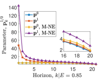
(a)

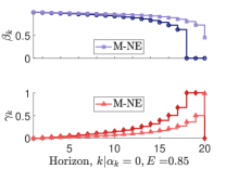
(b)

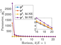
(c)

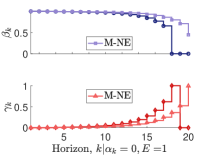
(d)

Figure 1: Saddle-point value parameters $\mathbf{p}_{k}^{i},k\in\{1,2,\dots,L\},i\in\{0,1\}$ for state transition constant (a) $E=0.85$, (c) $E=1.0$. The parameters $\mathbf{p}_{k}^{i},$M-NE corresponds to the parameters of the saddle-point under a mixed NE takeover over the entire time horizon. Defender takeover strategies $\beta_{k}$ and adversary takeover strategies $\gamma_{k}$ for state transition (b) $E=0.85$ and (d) $E=1.0$. M-NE corresponds to the mixed NE policy.

IV-C n-dimensional system

Unlike the scalar case, wherein the state $x$ was factored out during the computation of the NE takeover strategies and saddle-point value parameters $\mathbf{p}_{k}^{0}$ and $\mathbf{p}_{k}^{1}$, that simplification does not yield exact results for an $n-$dimensional system. The challenge for factoring out the state at any time $k\in\mathcal{K}$, arises from the term

$$\dfrac{x^{\text{T}}a_{k}\mathbb{I}_{n}xx^{\text{T}}d_{k}\mathbb{I}_{n}x}{\underbrace{x^{\text{T}}\left(\check{W}_{k}(\eta_{k})^{\text{T}}P^{1}_{k+1}\check{W}_{k}(\eta_{k})-\check{B}_{k}(\eta_{k})^{\text{T}}P^{0}_{k+1}\check{B}_{k}(\eta_{k})\right)x}_{\widetilde{P}_{k+1}(x)}},$$ (61)

which arises when a mixed strategy NE takeover is played in either of the FlipDyn states. A similar challenge was encountered in [27], where the aforementioned term was approximated to factor out the state $x$ while computing the saddle-point value parameters backward in time. Here, we propose a more general approach by leveraging the results of Theorem 2 to address this limitation. Recall that the parameterized control policy pair $\{u_{k}^{*}(\eta_{k}),w_{k}^{*}(\eta_{k})\}$ with a feasible parameter $\eta_{k}$ must satisfy condition (36):

$$x^{\text{T}} \left(\check{W}_{k}(\eta_{k})^{\text{T}}P^{1}_{k+1}\check{W}_{k}(\eta_{k})-\right.$$

$$\left.\check{B}_{k}(\eta_{k})^{\text{T}}P^{0}_{k+1}\check{B}_{k}(\eta_{k})\right)x=x^{\text{T}}x\dfrac{\sqrt{a_{k}d_{k}}}{\eta_{k}}.$$

Substituting condition (36) in (61) yields:

$$\dfrac{x^{\text{T}}a_{k}\mathbb{I}_{n}xx^{\text{T}}d_{k}\mathbb{I}_{n}x}{\widetilde{P}_{k+1}(x)}:=\dfrac{\eta_{k}x^{\text{T}}a_{k}\mathbb{I}_{n}xx^{\text{T}}d_{k}\mathbb{I}_{n}x}{x^{\text{T}}x\sqrt{a_{k}d_{k}}}=\eta_{k}\sqrt{a_{k}d_{k}}x^{\text{T}}x.$$ (62)

Analogous to the scalar/$1-$dimensional case, we will use Theorem 1 to present the following result, which provides a closed-form expression for the NE takeover in both pure and mixed strategies of both players, and outlines the saddle-point value update of the parameter $P_{k}^{\alpha}\in\mathbb{R}^{n\times n},\alpha\in\{0,1\}$.

Corollary 2

(Case $\alpha_{k}=0$) The unique NE takeover strategies of the FlipDyn-Con game (7) for every $k\in\mathcal{K}$, subject to the dynamics (51), with quadratic costs (25), takeover costs (30), and FlipDyn dynamics (3) are given by

$$\begin{split}y^{0*}_{k}=\begin{cases}\begin{bmatrix}\eta_{k}\sqrt{\cfrac{a_{k}}{d_{k}}}&1-\eta_{k}\sqrt{\cfrac{a_{k}}{d_{k}}}\end{bmatrix}^{\text{T}},\hfill\text{if }\begin{matrix}\widetilde{P}_{k+1}(x)>x^{\text{T}}a_{k}\mathbb{I}_{n}x,\\ \widetilde{P}_{k+1}(x)>x^{\text{T}}d_{k}\mathbb{I}_{n}x,\end{matrix}\\ \begin{bmatrix}\hphantom{00}1&\hphantom{a_{k}0000000}0\hphantom{000}\end{bmatrix}^{\text{T}},\ \text{otherwise,}\end{cases}\end{split}$$ (63)

$$\begin{split}z^{0*}_{k}=\begin{cases}\begin{bmatrix}1-\eta_{k}\sqrt{\cfrac{d_{k}}{a_{k}}}&\eta_{k}\sqrt{\cfrac{d_{k}}{a_{k}}}\end{bmatrix}^{\text{T}},&\text{if }\begin{matrix}\widetilde{P}_{k+1}(x)>x^{\text{T}}a_{k}\mathbb{I}_{n}x,\\ \widetilde{P}_{k+1}(x)>x^{\text{T}}d_{k}\mathbb{I}_{n}x,\end{matrix}\\ \begin{bmatrix}\hphantom{00}0&\hphantom{a_{k}0000000}1\hphantom{000}\end{bmatrix}^{\text{T}},&\text{if }\begin{matrix}\widetilde{P}_{k+1}(x)>x^{\text{T}}a_{k}\mathbb{I}_{n}x,\\ \widetilde{P}_{k+1}(x)\leq x^{\text{T}}d_{k}\mathbb{I}_{n}x,\end{matrix}\\ \begin{bmatrix}\hphantom{00}1&\hphantom{a_{k}0000000}0\hphantom{000}\end{bmatrix}^{\text{T}},&\text{otherwise.}\end{cases}\end{split}$$ (64)

The saddle-point value parameter at time $k$ is given by:

$$P_{k}^{0}=\begin{cases}\begin{aligned} &G^{0}_{k}+\check{B}_{k}(\eta_{k})^{\text{T}}P^{0}_{k+1}\check{B}_{k}(\eta_{k})\\[1.0pt] &+K_{k}^{*}(\eta_{k})^{\text{T}}M_{k}K_{k}^{*}(\eta_{k})\\[1.0pt] &+d_{k}\mathbb{I}_{n}-\mathbb{I}_{n}\eta_{k}\sqrt{a_{k}d_{k}},\end{aligned}&\text{if }\begin{matrix}\widetilde{P}_{k+1}(x)>x^{\text{T}}a_{k}\mathbb{I}_{n}x,\\ \widetilde{P}_{k+1}(x)>x^{\text{T}}d_{k}\mathbb{I}_{n}x,\end{matrix}\\[15.0pt] \begin{aligned} &G^{0}_{k}+\check{W}_{k}(\eta_{k})^{\text{T}}{P}^{1}_{k+1}\check{W}_{k}(\eta_{k})\\ &-a_{k}\mathbb{I}_{n},\end{aligned}&\text{if }\begin{matrix}\widetilde{P}_{k+1}(x)>x^{\text{T}}a_{k}\mathbb{I}_{n}x,\\ \widetilde{P}_{k+1}(x)\leq x^{\text{T}}d_{k}\mathbb{I}_{n}x,\end{matrix}\\[15.0pt] \begin{aligned} &G^{0}_{k}+K_{k}^{*}(0)^{\text{T}}M_{k}K_{k}^{*}(0)\\[1.0pt] &+\check{B}_{k}(0)^{\text{T}}P^{0}_{k+1}\check{B}_{k}(0),\end{aligned}&\text{otherwise}.\end{cases}$$ (65)

(Case $\alpha_{k}=1$) The unique NE takeover strategies are given by:

$$\begin{split}y^{1*}_{k}=\begin{cases}\begin{bmatrix}1-\eta_{k}\sqrt{\cfrac{a_{k}}{d_{k}}}&\eta_{k}\sqrt{\cfrac{a_{k}}{d_{k}}}\end{bmatrix}^{\text{T}},&\text{if }\ \begin{matrix}\widetilde{P}_{k+1}(x)>x^{\text{T}}a_{k}\mathbb{I}_{n}x,\\ \widetilde{P}_{k+1}(x)>x^{\text{T}}d_{k}\mathbb{I}_{n}x,\end{matrix}\\ \begin{bmatrix}\hphantom{0000}0&\hphantom{a_{k}000000}1\hphantom{00}\end{bmatrix}^{\text{T}},&\text{if }\ \begin{matrix}\widetilde{P}_{k+1}(x)\leq x^{\text{T}}a_{k}\mathbb{I}_{n}x,\\ \widetilde{P}_{k+1}(x)>x^{\text{T}}d_{k}\mathbb{I}_{n}x,\end{matrix}\\ \begin{bmatrix}\hphantom{0000}1&\hphantom{a_{k}000000}0\hphantom{00}\end{bmatrix}^{\text{T}},&\text{otherwise,}\end{cases}\end{split}$$ (66)

$$\begin{split}z^{1*}_{k}=\begin{cases}\begin{bmatrix}\eta_{k}\sqrt{\cfrac{d_{k}}{a_{k}}}&1-\eta_{k}\sqrt{\cfrac{d_{k}}{a_{k}}}\end{bmatrix}^{\text{T}},&\text{if }\ \begin{matrix}\widetilde{P}_{k+1}(x)>x^{\text{T}}a_{k}\mathbb{I}_{n}x,\\ \widetilde{P}_{k+1}(x)>x^{\text{T}}d_{k}\mathbb{I}_{n}x,\end{matrix}\\ \begin{bmatrix}\hphantom{0000}1&\hphantom{a_{k}000000}0\hphantom{00}\end{bmatrix}^{\text{T}},&\text{otherwise}.\end{cases}\end{split}$$ (67)

The saddle-point value parameter at time $k$ is given by,

$$P_{k}^{1}=\begin{cases}\begin{aligned} &G^{1}_{k}+\check{W}_{k}(\eta_{k})^{\text{T}}P^{1}_{k+1}\check{W}_{k}(\eta_{k})\\[1.0pt] &-W_{k}^{\text{T}*}(\eta_{k})N_{k}W_{k}^{*}(\eta_{k})\\[1.0pt] &-a_{k}\mathbb{I}_{n}+\mathbb{I}_{n}\eta_{k}\sqrt{a_{k}d_{k}},\end{aligned}&\text{if }\begin{matrix}\widetilde{P}_{k+1}(x)>x^{\text{T}}a_{k}\mathbb{I}_{n}x,\\ \widetilde{P}_{k+1}(x)>x^{\text{T}}d_{k}\mathbb{I}_{n}x,\end{matrix}\\[15.0pt] \begin{aligned} &G^{1}_{k}+\check{B}_{k}(\eta_{k})^{\text{T}}P^{0}_{k+1}\check{B}_{k}(\eta_{k})\\ &+d_{k}\mathbb{I}_{n},\end{aligned}&\text{if }\begin{matrix}\widetilde{P}_{k+1}(x)\leq x^{\text{T}}a_{k}\mathbb{I}_{n}x,\\ \widetilde{P}_{k+1}(x)>x^{\text{T}}d_{k}\mathbb{I}_{n}x,\end{matrix}\\[15.0pt] \begin{aligned} &G^{1}_{k}-W_{k}(0)^{\text{T}*}N_{k}W_{k}^{*}(0)\\ &+\check{W}_{k}(0)^{\text{T}}P^{1}_{k+1}\check{W}_{k}(0),\end{aligned}&\text{otherwise}.\end{cases}$$ (68)

The recursions (65) and (68) hold provided,

$$B_{k}^{\text{T}}P_{k+1}^{0}B_{k}+M_{k}\succ 0,\ H_{k}^{\text{T}}P_{k+1}^{1}H_{k}-N_{k}\prec 0.$$ (69)

The terminal conditions for the recursions (65) and (68) are:

$$P_{L+1}^{0}:=G_{L+1}^{0},\quad P_{L+1}^{1}:=G_{L+1}^{1}.$$

$\Box$

Proof:

We begin the proof by determining the NE takeover in pure and mixed strategies of the FlipDyn state of $\alpha=0$. We substitute the takeover cost (30) and the terms from (62) in (14) and (15), to obtain the NE takeover policies in (63) and (64), respectively. Analogous to the scalar/$1-$dimensional case, the NE takeover strategies in (66) and (67) for the FlipDyn state of $\alpha=1$ are the complementary takeover strategies of the FlipDyn state $\alpha=0$.

To determine the saddle-point value parameters for the FlipDyn state of $\alpha=0$, we substitute (62), discrete-time linear dynamics (51), quadratic costs (25) and takeover costs (30) in (16) and factor out the state $x$ to obtain (65). Through similar substitutions and factorization we can obtain (68) corresponding to the FlipDyn state of $\alpha=1$.  $\Box$

Similar to the $1-$dimensional case, Corollary 2 presents a closed-form solution for the FlipDyn-Con (7) game with NE takeover strategies independent of state. However, this NE takeover strategy and saddle-point value parameters are conditioned on finding a feasible parameter $\eta_{k},\forall k\in\mathcal{K}$ that satisfies (62). A feasible parameter $\eta_{k}$ is seldom found corresponding to the linear dynamics (51), as the matrices $\check{B}_{k}(\zeta_{k})$ and $\check{W}_{k}(\zeta_{k})$ are generally non-diagonal. Therefore, there is a need to find approximate NE takeover strategies and bounds on the saddle-point values for any general $n-$dimensional case which need not satisfy (62). A solution addressing the limitation in determining a parameter $\eta_{k}$ is found by re-visiting the optimal linear state-feedback control from Theorem 2, described in the following result.

Lemma 1

Under Assumptions 2 and 3, consider a linear dynamical system described by (24) with quadratic costs (25), takeover costs (30), and FlipDyn dynamics (3) with known saddle-point value parameters $P^{1}_{k+1}$ and $P^{0}_{k+1}$. Suppose that for every $k\in\mathcal{K}$,

$$B_{k}^{\text{T}}P_{k+1}^{0}B_{k}+M_{k}\succ 0,\quad H_{k}^{\text{T}}P_{k+1}^{1}H_{k}-N_{k}\prec 0,$$ (70)

and for every $x\in\mathcal{X}$, there exists scalars $\underline{\eta}_{k}\in\mathbb{R}$ and $\overline{\eta}_{k}\in\mathbb{R}$ which correspond to an optimal linear state-feedback control pair $\{K_{k}^{*}(\underline{\eta}_{k}),W_{k}^{*}(\overline{\eta}_{k})\}$ of the form (32) and (33), such the following conditions are satisfied:

$$x^{\text{T}}x\dfrac{\sqrt{a_{k}d_{k}}}{\underline{\eta}_{k}}\leq x^{\text{T}}\mathbf{P}_{k+1}x\leq x^{\text{T}}x\dfrac{\sqrt{a_{k}d_{k}}}{\overline{\eta}_{k}},$$ (71)

$$(E_{k}+H_{k}W_{k}^{*}(\overline{\eta}_{k}))^{\text{T}}P_{k+1}^{1}(E_{k}+H_{k}W_{k}^{*}(\overline{\eta}_{k}))$$ (72)

$$-(E_{k}+B_{k}K_{k}^{*}(\underline{\eta}_{k}))^{\text{T}}P_{k+1}^{0}(E_{k}+B_{k}K_{k}^{*}(\underline{\eta}_{k}))\succ d_{k}\mathbb{I}_{n},$$

$$(E_{k}+H_{k}W_{k}^{*}(\overline{\eta}_{k}))^{\text{T}}P_{k+1}^{1}(E_{k}+H_{k}W_{k}^{*}(\overline{\eta}_{k}))$$ (73)

$$-(E_{k}+B_{k}K_{k}^{*}(\underline{\eta}_{k}))^{\text{T}}P_{k+1}^{0}(E_{k}+B_{k}K_{k}^{*}(\underline{\eta}_{k}))\succ a_{k}\mathbb{I}_{n}.$$

where

$$\mathbf{P}_{k+1}= (E_{k}+H_{k}W_{k}^{*}(\overline{\eta}_{k}))^{\text{T}}P_{k+1}^{1}(E_{k}+H_{k}W_{k}^{*}(\overline{\eta}_{k}))-$$

$$(E_{k}+B_{k}K_{k}^{*}(\underline{\eta}_{k}))^{\text{T}}P_{k+1}^{0}(E_{k}+B_{k}K_{k}^{*}(\underline{\eta}_{k})).$$

Then, the saddle-point value parameters at time $k\in\mathcal{K}$, under a mixed strategy NE takeover of both the FlipDyn states satisfy

$$P_{k}^{0}\preceq\begin{aligned} &G^{0}_{k}+d_{k}\mathbb{I}_{n}+K_{k}^{*}(\underline{\eta}_{k})^{\text{T}}M_{k}K_{k}^{*}(\underline{\eta}_{k})-\mathbb{I}_{n}\underline{\eta}_{k}\sqrt{a_{k}d_{k}}\\ &+\check{B}_{k}(\underline{\eta}_{k})^{\text{T}}P^{0}_{k+1}\check{B}_{k}(\underline{\eta}_{k}),\end{aligned}$$ (74)

$$P_{k}^{1}\succeq\begin{aligned} &G^{1}_{k}-a_{k}\mathbb{I}_{n}-W_{k}^{*}(\overline{\eta}_{k})^{\text{T}}N_{k}W_{k}^{*}(\overline{\eta}_{k})+\mathbb{I}_{n}\overline{\eta}_{k}\sqrt{a_{k}d_{k}}\\ &+\check{W}_{k}(\overline{\eta}_{k})^{\text{T}}P^{1}_{k+1}\check{W}_{k}(\overline{\eta}_{k}).\end{aligned}$$ (75)

$\Box$

Proof:

From (32), a linear defender control policy gain parameterized by a scalar $\underline{\eta}_{k}$, is given by:

$$K_{k}^{*}(\underline{\eta}_{k})=-(\vartheta(\underline{\eta}_{k})B_{k}^{\text{T}}P_{k+1}^{0}B_{k}+M_{k})^{-1}(\vartheta(\underline{\eta}_{k})B_{k}^{\text{T}}P_{k+1}^{0}E_{k}),$$ (76)

where $\vartheta(c):=1-c^{2}$. Likewise, from (33), a linear adversary control policy gain parameterized by a scalar $\overline{\eta}_{k}$, is given by:

$$W_{k}^{*}(\overline{\eta}_{k})=-(\vartheta(\overline{\eta}_{k})H_{k}^{\text{T}}P_{k+1}^{1}H_{k}-N_{k})^{-1}(\vartheta(\overline{\eta}_{k})H_{k}^{\text{T}}P_{k+1}^{1}E_{k}).$$ (77)

Upon substituting the condition (71) in (37) and (38) and solving for the second-order optimality condition (similar to Theorem 2) yields (70), which certifies a saddle-point equilibrium.

Recall that any control policy pair $\{K_{k},W_{k}\}$ that constitutes a mixed strategy NE takeover to both the saddle-point values $V_{k}^{0}(x)$ and $V_{k}^{1}(x)$ must satisfy the conditions:

$$\widetilde{P}_{k+1}(x)>d_{k}x^{\text{T}}x,\ \widetilde{P}_{k+1}(x)>a_{k}x^{\text{T}}x.$$

Thus, upon substituting the linear dynamics (24) and the optimal control gains $\{K_{k}^{*}(\underline{\eta}_{k}),W_{k}^{*}(\overline{\eta}_{k})\}$ in (28) and factoring out the state $x$, we obtain the conditions (72) and (73).

Next, we will only establish (74), as the derivation for (75) is analogous. Under a mixed strategy NE takeover, we substitute the quadratic costs (25), discrete-time linear dynamics (51) and the defender control (76) in (16) to obtain:

$$x^{\text{T}}P_{k}^{0}x= x^{\text{T}}\left(G^{0}_{k}+d_{k}\mathbb{I}_{n}+K_{k}^{*}(\underline{\eta}_{k})^{\text{T}}M_{k}K_{k}^{*}(\underline{\eta}_{k})\right)x+$$

$$x^{\text{T}}\left(\check{B}_{k}(\underline{\eta}_{k})^{\text{T}}P^{0}_{k+1}\check{B}_{k}(\underline{\eta}_{k})\right)x-$$

$$\dfrac{x^{\text{T}}a_{k}\mathbb{I}_{n}xx^{\text{T}}d_{k}\mathbb{I}_{n}x}{x^{\text{T}}\underbrace{\left(\check{W}_{k}(\overline{\eta}_{k})^{\text{T}}P^{1}_{k+1}\check{W}_{k}(\overline{\eta}_{k})-\check{B}_{k}(\underline{\eta}_{k})^{\text{T}}P^{0}_{k+1}\check{B}_{k}(\underline{\eta}_{k})\right)}_{\mathbf{P}_{k+1}}x}.$$

Using condition (71), we bound the term containing $\mathbf{P}_{k+1}$ by

$$\dfrac{x^{\text{T}}a_{k}\mathbb{I}_{n}xx^{\text{T}}d_{k}\mathbb{I}_{n}x}{x^{\text{T}}\mathbf{P}_{k+1}x} \leq\underline{\eta}_{k}\dfrac{x^{\text{T}}a_{k}\mathbb{I}_{n}xx^{\text{T}}d_{k}\mathbb{I}_{n}x}{x^{\text{T}}x\sqrt{a_{k}d_{k}}},$$

$$\leq\underline{\eta}_{k}x^{\text{T}}x\sqrt{a_{k}d_{k}}.$$

Substituting this bound in $x^{\text{T}}P_{k}^{0}x$ and factoring out the state $x$, we obtain (74).

$\Box$

Lemma 1 provides a linear state-feedback control for the defender (resp. adversary) and enables us to compute bounds on the saddle-point values independent of the state $x$ backward in time. More importantly, condition (71) serves as a relaxation for (62). Such a relaxation enables us to determine an upper and lower bound in a semi-definite sense, for the saddle-point value parameters using the scalars $\overline{\eta}_{k}$ and $\underline{\eta}_{k}$, which can be used to approximately compute the saddle-point value parameters recursively. Therefore, following the same methodology from [27], for the $n-$dimensional case, we will solve for an approximate NE takeover strategies and saddle-point values using the parameterization,

$$\overline{V}_{k}^{0}(x):=x^{\text{T}}\overline{P}_{k}^{0}x,\quad\overline{V}_{k}^{1}(x):=x^{\text{T}}\overline{P}_{k}^{1}x,$$ (78)

where $\overline{P}_{k}^{1}\in\mathbb{R}^{n\times n}$ and $\overline{P}_{k}^{0}\in\mathbb{R}^{n\times n}$.

As shown in Corollary 2, we will use the results from Theorem 1 to provide an approximate NE takeover pair $\{\overline{y}_{k}^{\alpha*},\overline{z}_{k}^{\alpha*}\}$, in both pure and mixed strategies of both players, and the corresponding approximate saddle-point value update of the parameter $\overline{P}_{k}^{\alpha}\in\mathbb{R}^{n\times n},\alpha\in\{0,1\}$.

Corollary 3

(Case $\alpha_{k}=0$) The approximate NE takeover strategies of the FlipDyn-Con game (7) at any time $k\in\mathcal{K}$, subject to dynamics in (51), with quadratic costs (25), takeover costs (30), and FlipDyn dynamics (3) are given by:

$$\begin{split}\overline{y}^{0*}_{k}=\begin{cases}\begin{bmatrix}\cfrac{a_{k}x^{\text{T}}x}{x^{\text{T}}\overline{\mathbf{P}}_{k+1}x}&1-\cfrac{a_{k}x^{\text{T}}x}{x^{\text{T}}\overline{\mathbf{P}}_{k+1}x}\end{bmatrix}^{\text{T}},\ \text{if }\begin{matrix}\widetilde{P}_{k+1}(x)>a_{k}x^{\text{T}}x,\\ \widetilde{P}_{k+1}(x)>d_{k}x^{\text{T}}x,\end{matrix}\\ \begin{bmatrix}\hphantom{00}1&\hphantom{a_{k}0000000000}0\hphantom{000}\end{bmatrix}^{\text{T}},\ \text{otherwise,}\end{cases}\end{split}$$ (79)

$$\begin{split}\overline{z}^{0*}_{k}=\begin{cases}\begin{bmatrix}1-\cfrac{d_{k}x^{\text{T}}x}{x^{\text{T}}\overline{\mathbf{P}}_{k+1}x}&\cfrac{d_{k}x^{\text{T}}x}{x^{\text{T}}\overline{\mathbf{P}}_{k+1}x}\end{bmatrix}^{\text{T}},\ \text{if }\begin{matrix}\widetilde{P}_{k+1}(x)>a_{k}x^{\text{T}}x,\\ \widetilde{P}_{k+1}(x)>d_{k}x^{\text{T}}x,\end{matrix}\\ \begin{bmatrix}\hphantom{0000}0&\hphantom{a_{k}00000000}1\hphantom{000}\end{bmatrix}^{\text{T}},\ \text{if }\begin{matrix}\widetilde{P}_{k+1}(x)>a_{k}x^{\text{T}}x,\\ \widetilde{P}_{k+1}(x)\leq d_{k}x^{\text{T}}x,\end{matrix}\\ \begin{bmatrix}\hphantom{0000}1&\hphantom{a_{k}00000000}0\hphantom{000}\end{bmatrix}^{\text{T}},\ \text{otherwise,}\end{cases}\end{split}$$ (80)

where

$$\overline{\mathbf{P}}_{k+1}:=\check{W}_{k}(\overline{\eta}_{k})^{\text{T}}\overline{P}^{1}_{k+1}\check{W}_{k}(\overline{\eta}_{k})-\check{B}_{k}(\underline{\eta}_{k})^{\text{T}}\overline{P}^{0}_{k+1}\check{B}_{k}(\underline{\eta}_{k}),$$

and $\widetilde{P}_{k+1}(x):=x^{\text{T}}\overline{\mathbf{P}}_{k+1}x$.

The approximate saddle-point value parameter at time $k$ is given by:

$$\overline{P}_{k}^{0}=\begin{cases}\begin{aligned} &G^{0}_{k}+\check{B}_{k}(\underline{\eta}_{k})^{\text{T}}\overline{P}^{0}_{k+1}\check{B}_{k}(\underline{\eta}_{k})\\[1.0pt] &+K_{k}^{*}(\underline{\eta}_{k})^{\text{T}}M_{k}K_{k}^{*}(\underline{\eta}_{k})\\[1.0pt] &+d_{k}\mathbb{I}_{n}-\mathbb{I}_{n}\underline{\eta}_{k}\sqrt{a_{k}d_{k}},\end{aligned}\ \text{if }\begin{matrix}\widetilde{P}_{k+1}(x)>a_{k}x^{\text{T}}x,\\ \widetilde{P}_{k+1}(x)>d_{k}x^{\text{T}}x,\end{matrix}\\[15.0pt] \begin{aligned} &G^{0}_{k}+\check{W}_{k}(\overline{\eta}_{k})^{\text{T}}\overline{P}^{1}_{k+1}\check{W}_{k}(\overline{\eta}_{k})\\ &-a_{k}\mathbb{I}_{n},\end{aligned}\ \text{if }\begin{matrix}\widetilde{P}_{k+1}(x)>a_{k}x^{\text{T}}x,\\ \widetilde{P}_{k+1}(x)\leq d_{k}x^{\text{T}}x,\end{matrix}\\[15.0pt] \begin{aligned} &G^{0}_{k}+K_{k}^{*}(0)^{\text{T}}M_{k}K_{k}^{*}(0)\\[1.0pt] &+\check{B}_{k}(0)^{\text{T}}\overline{P}^{0}_{k+1}\check{B}_{k}(0),\end{aligned}\ \qquad\text{otherwise}.\end{cases}$$ (81)

(Case $\alpha_{k}=1$) The approximate NE takeover strategies are given by:

$$\begin{split}\overline{y}^{1*}_{k}=\begin{cases}\begin{bmatrix}1-\cfrac{a_{k}x^{\text{T}}x}{x^{\text{T}}\overline{\mathbf{P}}_{k+1}x}&\cfrac{a_{k}x^{\text{T}}x}{x^{\text{T}}\overline{\mathbf{P}}_{k+1}x}\end{bmatrix}^{\text{T}},\ \text{if }\ \begin{matrix}\widetilde{P}_{k+1}(x)>a_{k}x^{\text{T}}x,\\ \widetilde{P}_{k+1}(x)>d_{k}x^{\text{T}}x,\end{matrix}\\ \begin{bmatrix}\hphantom{000000}0&\hphantom{a_{k}0000000}1\hphantom{00}\end{bmatrix}^{\text{T}},\ \text{if }\ \begin{matrix}\widetilde{P}_{k+1}(x)\leq a_{k}x^{\text{T}}x,\\ \widetilde{P}_{k+1}(x)>d_{k}x^{\text{T}}x,\end{matrix}\\ \begin{bmatrix}\hphantom{000000}1&\hphantom{a_{k}0000000}0\hphantom{00}\end{bmatrix}^{\text{T}},\ \text{otherwise,}\end{cases}\end{split}$$ (82)

$$\begin{split}\overline{z}^{1*}_{k}=\begin{cases}\begin{bmatrix}\dfrac{d_{k}x^{\text{T}}x}{x^{\text{T}}\overline{\mathbf{P}}_{k+1}x}&1-\dfrac{d_{k}x^{\text{T}}x}{x^{\text{T}}\overline{\mathbf{P}}_{k+1}x}\end{bmatrix}^{\text{T}},\ \text{if }\ \begin{matrix}\widetilde{P}_{k+1}(x)>a_{k}x^{\text{T}}x,\\ \widetilde{P}_{k+1}(x)>d_{k}x^{\text{T}}x,\end{matrix}\\ \begin{bmatrix}\hphantom{0000}1&\hphantom{a_{k}000000000}0\hphantom{00}\end{bmatrix}^{\text{T}},\ \text{otherwise.}\end{cases}\end{split}$$ (83)

The approximate saddle-point value parameter at time $k$ is given by,

$$\overline{P}_{k}^{1}=\begin{cases}\begin{aligned} &G^{1}_{k}+\check{W}_{k}(\overline{\eta}_{k})^{\text{T}}\overline{P}^{1}_{k+1}\check{W}_{k}(\overline{\eta}_{k})\\[1.0pt] &-W_{k}^{*}(\overline{\eta}_{k})^{\text{T}}N_{k}W_{k}^{*}(\overline{\eta}_{k})\\[1.0pt] &-a_{k}\mathbb{I}_{n}+\mathbb{I}_{n}\overline{\eta}_{k}\sqrt{a_{k}d_{k}},\end{aligned}\ \text{if }\begin{matrix}\widetilde{P}_{k+1}(x)>a_{k}x^{\text{T}}x,\\ \widetilde{P}_{k+1}(x)>d_{k}x^{\text{T}}x,\end{matrix}\\[10.0pt] \begin{aligned} &G^{1}_{k}+\check{B}_{k}(\underline{\eta}_{k})^{\text{T}}\overline{P}^{0}_{k+1}\check{B}_{k}(\underline{\eta}_{k})\\ &+d_{k}\mathbb{I}_{n},\end{aligned}\ \text{if }\begin{matrix}\widetilde{P}_{k+1}(x)\leq a_{k}x^{\text{T}}x,\\ \widetilde{P}_{k+1}(x)>d_{k}x^{\text{T}}x,\end{matrix}\\[10.0pt] \begin{aligned} &G^{1}_{k}-W_{k}(0)^{\text{T}*}N_{k}W_{k}^{*}(0)\\ &+\check{W}_{k}(0)^{\text{T}}\overline{P}^{1}_{k+1}\check{W}_{k}(0),\end{aligned}\ \text{otherwise}.\end{cases}$$ (84)

The recursions (81) and (84) hold provided,

$$B_{k}^{\text{T}}\overline{P}_{k+1}^{0}B_{k}+M_{k}\succ 0,\ H_{k}^{\text{T}}\overline{P}_{k+1}^{1}H_{k}-N_{k}\prec 0.$$ (85)

The terminal conditions for the recursions (81) and (84) are:

$$\overline{P}_{L+1}^{0}:=G_{L+1}^{0},\quad\overline{P}_{L+1}^{1}:=G_{L+1}^{1}.$$

$\Box$

Proof:

[Outline] Similar to the proofs in the prior sections, we begin the proof by determining the NE takeover in pure and mixed strategies for the FlipDyn state of $\alpha=0$. We substitute the quadratic costs (25), linear dynamics (51), and linear control gains (76) and (77) in the term $\widetilde{P}_{k+1}(x)$ with the approximate saddle-point value parameters $\overline{P}_{k+1}^{0}$ and $\overline{P}_{k+1}^{1}$ from (28) to obtain:

$$\tilde{P}_{k+1}(x) :=\overline{V}_{k+1}^{1}(\check{W}_{k}(\overline{\eta}_{k})x)-\overline{V}_{k+1}^{0}(\check{B}_{k}(\underline{\eta}_{k})x),$$

$$=x^{\text{T}}\left(\check{W}_{k}^{\text{T}}(\overline{\eta}_{k})\overline{P}_{k+1}^{1}\check{W}_{k}(\overline{\eta}_{k})\right.$$

$$\hphantom{=\mathbf{p}_{k+1}^{1}}\left.-\check{B}_{k}(\underline{\eta}_{k})^{\text{T}}\overline{P}_{k+1}^{0}\check{B}_{k}(\underline{\eta}_{k})\right)x,$$

$$=x^{\text{T}}\overline{\mathbf{P}}_{k+1}x.$$

We substitute the takeover cost (30) and $x^{\text{T}}\overline{\mathbf{P}}_{k+1}x$ in (14) and (15), to obtain the NE takeover policies in (79) and (80), respectively. The approximate NE takeover strategies of the FlipDyn state $\alpha=1$ are complementary to $\alpha=0$, presented in (82) and (83).

To determine the approximate saddle-point value parameters under a mixed strategy NE takeover of the FlipDyn state of $\alpha=0$, we substitute the upper bound (74) from Lemma 1 and replace $P_{k+1}^{0}$ with $\overline{{P}}_{k+1}^{0}$. Under a pure strategy NE takeover, we substitute the quadratic costs (25), discrete-time linear dynamics (51) and the adversary linear state-feedback control  (77) to obtain the approximate saddle-point value parameters. Combining both the solutions from the mixed and pure strategy NE takeover, we obtain (81).  $\Box$

Recursions (81) and (84) provide an approximate solution to the FlipDyn-Con problem (7) for the $n$-dimensional case with corresponding takeover and control policies. Similar to the range of the parameter $\eta_{k}$ presented in Lemma 1, the parameters $\overline{\eta}_{k}$ and $\underline{\eta}_{k}$ under a mixed strategy NE takeover can be bounded using condition (36), indicated in the following remark.

Remark 4

The permissible range for the parameters $\overline{\eta}_{k}$ and $\underline{\eta}_{k}$ satisfying condition (71) corresponding to a mixed strategy NE are given by:

$$0<\overline{\eta}_{k}\leq\eta_{k}\leq\underline{\eta}_{k}<\sqrt{\dfrac{\min_{\{d_{k},a_{k}\}}}{\max_{\{d_{k},a_{k}\}}}}<1.$$ (86)

Remark 4 is a direct consequence of Lemma 1. Similar to the scalar/$1-$dimensional case, not all control costs (25) satisfy the approximate saddle-point recursion. The following remark provides the minimum adversarial control cost required to satisfy the recursions (81) and (84).

Remark 5

Given an $n-$dimensional system (51) with quadratic costs (52), the NE takeover strategies and the recursion for the approximate saddle-point value parameter, as outlined in Corollary 3, exists for an adversary control costs $N^{*}_{k}{\prec}N_{k}$ provided

$$-N^{*}_{k}+H^{\text{T}}_{k}\overline{P}_{k+1}^{1}H_{k}{\prec}\,0,\quad\forall k\in\mathcal{K}.$$

Analogous to the scalar/$1-$dimensional system, the parameter $N^{*}_{k}$ can be found using a bisection method at every stage $k\in\mathcal{K}$. A candidate initial value for all $k\in\mathcal{K}$ can be set to $N_{L}:=\nu_{\mathbb{R}_{>0}}\mathbb{I}_{p}$ such that $\nu\mathbb{I}_{p}\succ H^{\text{T}}_{L}\overline{P}_{L+1}^{1}H_{L}$. Similarly, we can also determine a minimum adversarial state cost $G_{k}^{1*}$ to guarantee a mixed strategy NE takeover at every time $k$ for the $n$-dimensional system. The following remark summarizes such an adversarial cost.

Remark 6

Given a $n-$dimensional system (51) with quadratic costs (52), the mixed strategy NE takeover and the corresponding recursion for the approximate saddle-point value parameter, as outlined in Corollary 3, exists for an adversary state-dependent cost $G^{1*}_{k}\preceq G^{1}_{k}$ provided

$${\overline{\mathbf{P}}}_{k+1}\succ d_{k}\mathbb{I}_{n},\quad{\overline{\mathbf{P}}}_{k+1}\succ a_{k}\mathbb{I}_{n},\quad\forall k\in\mathcal{K},$$

with the parameters at the time $L+1$ given by:

$$\overline{P}_{L+1}^{1}:=G_{L+1}^{1*},\ \overline{P}_{L+1}^{0}:=G_{L+1}^{0}.$$ (87)

As indicated in the scalar/$1-$dimensional case, we can determine $G^{1*}_{k}$ using a bisection method, and simultaneously determine $G^{1*}_{k}$ and $N^{*}_{k}$ using a double bisection method. Next, we illustrate the results of the approximate value function on a numerical example.

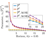
(a)

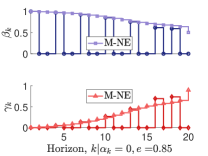
(b)

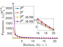
(c)

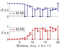
(d)

Figure 2: Maximum eigenvalues ($\lambda_{1}(\overline{P}_{k}^{\alpha})$) of saddle-point value parameters $\overline{P}_{k}^{\alpha},k\in\{0,1,\dots,L+1\},\alpha\in\{0,1\}$ for state transition constant (a) $e=0.85$, (c) $e=1.0$. The parameters $P_{k}^{i},$M-NE corresponds to saddle-point value parameter recursion under a mixed NE takeover over the entire time horizon. Defender takeover strategy $\beta_{k}$ and adversary takeover strategy $\gamma_{k}$ for state transition (b) $e=0.85$ and (d) $e=1.0$. M-NE corresponds to the mixed NE policy.

A Numerical Example

We now evaluate the results of the approximate NE takeover and the corresponding saddle-point value parameters presented in Corollary 3, on a discrete-time two-dimensional linear time-invariant system (LTI) for a horizon length of $L=20$. The quadratic costs (25) are assumed to be fixed $\forall k\in\mathcal{K}$, and are given by:

$$G^{0}_{k}=G^{0}=\mathbb{I}_{n},\ G^{1}_{k}=G^{1}= 1.35\mathbb{I}_{n},\ D_{k}=D=0.45\mathbb{I}_{n},$$

$$A_{k}=A=0.25\mathbb{I}_{n}, \ M_{k}=M=0.65.$$

The system transition matrix $E_{k}=E$ and control matrices for the defender and adversary are given by:

$$E_{k}=E=\begin{bmatrix}e&\Delta t\\ 0&e\end{bmatrix},B_{k}=H_{k}=\begin{bmatrix}\Delta t\\ 0\end{bmatrix},\quad\forall k\in\mathcal{K},$$

where $\Delta t=0.1$ for the numerical example. Similar to the scalar/$1-$dimensional case, we solve for the approximate NE takeover strategies and saddle-point value function parameters for two cases with a fixed state transition constant $e_{k}=e,\forall k\in\mathcal{K}$: $e=0.85$ and $1.0$. Since the saddle-point value parameters for $n$-dimensions are symmetric positive definite matrices, we plot the maximum eigenvalues of the value function matrices $\overline{P}_{k}^{1},\overline{P}_{k}^{0}$ shown in Figure 2a and 2c, with M-NE indicating a mixed strategy NE takeover over the entire horizon L, achieved through $N^{*}$ and $G^{1*}$. We obtain the adversary control costs $N_{k}^{*},\forall k\in\mathcal{K}$ for the case of $e=0.85$ given by:

$$N_{k}^{*}=N^{*}=\begin{cases}0.42,&\text{if }\begin{matrix}\overline{P}_{k+1}(x)\geq x^{\text{T}}a_{k}x,\\ \overline{P}_{k+1}(x)\geq x^{\text{T}}d_{k}x,\end{matrix}\\ 0.45,&\text{otherwise },\end{cases}$$

and for the case of $e=1.0$ as:

$$N_{k}^{*}=N^{*}=\begin{cases}3.73,&\text{if }\begin{matrix}\overline{P}_{k+1}(x)\geq x^{\text{T}}a_{k}x,\\ \overline{P}_{k+1}(x)\geq x^{\text{T}}d_{k}x,\end{matrix}\\ 3.40,&\text{otherwise. }\end{cases}$$

Similarly, we determine the minimum adversary cost $G_{k}^{1*}$ for each case of $e$, which corresponds to a mixed strategy NE takeover over the entire time horizon $L$ given by:

$$G^{1*}_{k}=G^{1*}=\begin{cases}1.67\mathbb{I}_{n},&\text{when }e=0.85,\\ 1.48\mathbb{I}_{n},&\text{when }e=1.00,\end{cases}$$

Similar to the scalar/$1-$dimensional case, we observe that the eigenvalues of the saddle-point value parameters are significantly lower when $e=0.85$ compared to $e=1.0$. This corresponds to lower incentives for a takeover when the system is open-loop stable $e<1$ as opposed to unstable condition of $e\geq 1$. However, the value function parameter $\overline{P}_{k}^{0}$ always reaches a steady-state value for either values $e$, implying that the system will remain stable under a defender’s control.

For the $n$-dimensional case, the takeover policy is a function of the state $x$. Therefore, we simulate the system for a total of 100 iterations with the initial state $x_{0}=\begin{bmatrix}1&0\end{bmatrix}^{\text{T}}$ and show the average takeover policies in Figure 2b and 2d. For the case of playing mixed NE takeover (M-NE), we observe for both $e=0.85$ and $e=1.0$, given $\alpha=0$, i.e., when the defender is in control, the probability of takeover for the defender (resp. adversary) increase (resp. decreases) backward in time. This takeover policy indicates that the defender retains control of the system while the adversary remains idle. For the case of playing between pure and mixed NE takeover, we observe that for both $e=0.85$ and $e=1.0$ given $\alpha=0$, both players alternate between pure and mixed NE over the horizon.

This numerical example illustrates the use of the approximate saddle-point value parameters in determining the takeover strategies for each player. Additionally, it provides insight into the system’s behavior for the given costs and the system’s stability properties. These insights are useful while designing the costs, which further impact the control and takeover policies.

V Conclusion and Future Directions

This paper introduced FlipDyn-Con, a finite-horizon, zero-sum game of resource takeovers involving a discrete-time dynamical system. Our contributions are distilled into four key facets. First, we presented analytical expressions for the saddle-point value of the FlipDyn-Con game, alongside the corresponding NE takeover in both the pure and mixed strategies. Second, we derived optimal control policies for linear dynamical systems characterized by quadratic costs. We provided sufficient conditions under which there is a saddle-point in the space of linear state-feedback policies. Third, for scalar/$1-$dimensional dynamical systems with quadratic costs, we derived exact saddle-point value parameters and NE takeover strategies, independent of the state of the dynamical system. Finally, for higher dimensional dynamical systems with quadratic costs, we provided approximate NE takeover strategies and control policies. Our approach enables computation for general linear systems, broadening its applicability. The practical implications of our findings were showcased through a numerical study involving the control of a linear dynamical system in the presence of an adversary.

Our future effort will focus on expanding the scope of our model. We aim to incorporate partial state observability, wherein the discrete FlipDyn state of the system needs to be estimated. We also plan to introduce bounded process and measurement noise into the framework, investigating its impact on the FlipDyn-Con game. We also plan to extend the number of FlipDyn states to more than two. Lastly, we intend to conduct a comparative study between our established solution and a learning-based approach, evaluating their performance across various objectives and cost functions.

References

References

• [1] R. Rajkumar, I. Lee, L. Sha, and J. Stankovic, “Cyber-physical systems: The next computing revolution,” in Design Automation Conference.   IEEE, 2010, pp. 731–736.
• [2] R. Baheti and H. Gill, “Cyber-physical systems,” The Impact of Control Technology, vol. 12, no. 1, pp. 161–166, 2011.
• [3] E. A. Lee and S. A. Seshia, Introduction to embedded systems: A cyber-physical systems approach.   MIT press, 2016.
• [4] A. A. Cárdenas, S. Amin, and S. Sastry, “Research challenges for the security of control systems,” in Proceedings of the 3rd Conference on Hot Topics in Security, ser. HOTSEC’08.   USA: USENIX Association, 2008.
• [5] S. Parkinson, P. Ward, K. Wilson, and J. Miller, “Cyber threats facing autonomous and connected vehicles: Future challenges,” IEEE Transactions on Intelligent Transportation Systems, vol. 18, no. 11, pp. 2898–2915, 2017.
• [6] Y. Z. Lun, A. D’Innocenzo, F. Smarra, I. Malavolta, and M. D. Di Benedetto, “State of the art of cyber-physical systems security: An automatic control perspective,” Journal of Systems and Software, vol. 149, pp. 174–216, 2019.
• [7] W. Tushar, C. Yuen, T. K. Saha, S. Nizami, M. R. Alam, D. B. Smith, and H. V. Poor, “A survey of cyber-physical systems from a game-theoretic perspective,” IEEE Access, vol. 11, pp. 9799–9834, 2023.
• [8] C. S. Wickramasinghe, D. L. Marino, K. Amarasinghe, and M. Manic, “Generalization of deep learning for cyber-physical system security: A survey,” in IECON 2018-44th Annual Conference of the IEEE Industrial Electronics Society.   IEEE, 2018, pp. 745–751.
• [9] A. Avizienis, J.-C. Laprie, B. Randell, and C. Landwehr, “Basic concepts and taxonomy of dependable and secure computing,” IEEE transactions on dependable and secure computing, vol. 1, no. 1, pp. 11–33, 2004.
• [10] M. Van Dijk, A. Juels, A. Oprea, and R. L. Rivest, “Flipit: The game of “stealthy takeover”,” Journal of Cryptology, vol. 26, no. 4, pp. 655–713, 2013.
• [11] K. D. Bowers, M. Van Dijk, R. Griffin, A. Juels, A. Oprea, R. L. Rivest, and N. Triandopoulos, “Defending against the unknown enemy: Applying flipit to system security,” in International Conference on Decision and Game Theory for Security.   Springer, 2012, pp. 248–263.
• [12] B. Johnson, A. Laszka, and J. Grossklags, “Games of timing for security in dynamic environments,” in Decision and Game Theory for Security: 6th International Conference, GameSec 2015, London, UK, November 4-5, 2015, Proceedings 6.   Springer, 2015, pp. 57–73.
• [13] A. Laszka, G. Horvath, M. Felegyhazi, and L. Buttyán, “FlipThem: Modeling targeted attacks with FlipIt for multiple resources,” in International Conference on Decision and Game Theory for Security.   Springer, 2014, pp. 175–194.
• [14] D. Leslie, C. Sherfield, and N. P. Smart, “Threshold flipthem: When the winner does not need to take all,” in Decision and Game Theory for Security: 6th International Conference, GameSec 2015, London, UK, November 4-5, 2015, Proceedings 6.   Springer, 2015, pp. 74–92.
• [15] M. Zhang, Z. Zheng, and N. B. Shroff, “A game theoretic model for defending against stealthy attacks with limited resources,” in Decision and Game Theory for Security: 6th International Conference, GameSec 2015, London, UK, November 4-5, 2015, Proceedings 6.   Springer, 2015, pp. 93–112.
• [16] ——, “Defending against stealthy attacks on multiple nodes with limited resources: A game-theoretic analysis,” IEEE Transactions on Control of Network Systems, vol. 7, no. 4, pp. 1665–1677, 2020.
• [17] E. Canzani and S. Pickl, “Cyber epidemics: Modeling attacker-defender dynamics in critical infrastructure systems,” in Advances in Human Factors in Cybersecurity: Proceedings of the AHFE 2016 International Conference on Human Factors in Cybersecurity, July 27-31, 2016, Walt Disney World®, Florida, USA.   Springer, 2016, pp. 377–389.
• [18] S. Saha, A. Vullikanti, and M. Halappanavar, “Flipnet: Modeling covert and persistent attacks on networked resources,” in 2017 IEEE 37th International Conference on Distributed Computing Systems (ICDCS).   IEEE, 2017, pp. 2444–2451.
• [19] Z. Liu and L. Wang, “Flipit game model-based defense strategy against cyberattacks on scada systems considering insider assistance,” IEEE Transactions on Information Forensics and Security, vol. 16, pp. 2791–2804, 2021.
• [20] J. Ding, M. Kamgarpour, S. Summers, A. Abate, J. Lygeros, and C. Tomlin, “A stochastic games framework for verification and control of discrete time stochastic hybrid systems,” Automatica, vol. 49, no. 9, pp. 2665–2674, 2013.
• [21] E. Dallal, D. Neider, and P. Tabuada, “Synthesis of safety controllers robust to unmodeled intermittent disturbances,” in 2016 IEEE 55th Conference on Decision and Control (CDC).   IEEE, 2016, pp. 7425–7430.
• [22] C. Fiscko, B. Swenson, S. Kar, and B. Sinopoli, “Control of parametric games,” in 2019 18th European Control Conference (ECC).   IEEE, 2019, pp. 1036–1042.
• [23] C. Fiscko, S. Kar, and B. Sinopoli, “Efficient solutions for targeted control of multi-agent mdps,” in 2021 American control conference (acc).   IEEE, 2021, pp. 690–696.
• [24] ——, “Cluster-based control of transition-independent mdps,” arXiv preprint arXiv:2207.05224, 2022.
• [25] Q. Zhu and T. Basar, “Game-theoretic methods for robustness, security, and resilience of cyberphysical control systems: games-in-games principle for optimal cross-layer resilient control systems,” IEEE Control Systems Magazine, vol. 35, no. 1, pp. 46–65, 2015.
• [26] E. Kontouras, A. Tzes, and L. Dritsas, “Adversary control strategies for discrete-time systems,” in 2014 European Control Conference (ECC).   IEEE, 2014, pp. 2508–2513.
• [27] S. Banik and S. D. Bopardikar, “Flipdyn: A game of resource takeovers in dynamical systems,” in 2022 IEEE 61st Conference on Decision and Control (CDC), 2022, pp. 2506–2511.
• [28] E. Kontouras, A. Tzes, and L. Dritsas, “Covert attack on a discrete-time system with limited use of the available disruption resources,” in 2015 European Control Conference (ECC).   IEEE, 2015, pp. 812–817.
• [29] R. S. Smith, “Covert misappropriation of networked control systems: Presenting a feedback structure,” IEEE Control Systems Magazine, vol. 35, no. 1, pp. 82–92, 2015.
• [30] A. M. Mohan, N. Meskin, and H. Mehrjerdi, “Covert attack in load frequency control of power systems,” in 2020 6th IEEE International Energy Conference (ENERGYCon).   IEEE, 2020, pp. 802–807.
• [31] J. P. Hespanha, Noncooperative game theory: An introduction for engineers and computer scientists.   Princeton University Press, 2017.
• [32] L. S. Shapley and R. Snow, “Basic solutions of discrete games,” Contributions to the Theory of Games, vol. 1, pp. 27–35, 1952.