Tightening QC Relaxations of AC Optimal Power Flow through Improved Linear Convex Envelopes

Abstract

AC optimal power flow (AC OPF) is a fundamental problem in power system operations. Accurately modeling the network physics via the AC power flow equations makes AC OPF a challenging nonconvex problem. To search for global optima, recent research has developed a variety of convex relaxations that bound the optimal objective values of AC OPF problems. The well-known QC relaxation convexifies the AC OPF problem by enclosing the non-convex terms (trigonometric functions and products) within convex envelopes. The accuracy of this method strongly depends on the tightness of these envelopes. This paper proposes two improvements for tightening QC relaxations of OPF problems. We first consider a particular nonlinear function whose projections are the nonlinear expressions appearing in the polar representation of the power flow equations. We construct a convex envelope around this nonlinear function that takes the form of a polytope and then use projections of this envelope to obtain convex expressions for the nonlinear terms. Second, we use certain characteristics of the sine and cosine expressions along with the changes in their curvature to tighten this convex envelope. We also propose a coordinate transformation that rotates the power flow equations by an angle specific to each bus in order to obtain a tighter envelope. We demonstrate these improvements relative to a state-of-the-art QC relaxation implementation using the PGLib-OPF test cases. The results show improved optimality gaps in 68% of these cases.

I Introduction

The optimal power flow (OPF) problem seeks an operating point that optimizes a specified objective function (often generation cost minimization) subject to constraints from the network physics and engineering limits. Using the nonlinear AC power flow model to accurately represent the power flow physics results in the AC OPF problem, which is non-convex, may have multiple local optima [1], and is generally NP-Hard [2]. Since it was first formulated by Carpentier in 1962 [3], a wide variety of algorithms have been applied to the OPF problem [4].

A plethora of research has focused on algorithms for obtaining locally optimal or approximate OPF solutions [5]. Recently, many convex relaxation techniques have been applied to OPF problems to obtain bounds on the optimal objective values, certify infeasibility, and in some cases, achieve globally optimal solutions. The objective value bounds are useful for determining how close a local solution is to being globally optimal. Thus, local algorithms and relaxations can be used together in spatial branch-and-bound methods [6]. Power flow relaxations are also valuable for a range of other applications, including solving robust OPF problems [7, 8], calculating voltage stability margins [9], exploring feasible operating ranges [10, 11], computing optimal switching decisions [12], etc. Convex relaxation methods are under active research with ongoing efforts targeting to improve their tightness. See [13] for a survey of power flow relaxations.

The well-known “Quadratic Convex” (QC) relaxation encloses the trigonometric, squared, and product terms in a polar representation of power flow equations within convex envelopes [14]. Since the quality of these envelopes determines the tightness of the QC relaxation, a number of research efforts have focused on improving these envelopes. These include tighter trigonometric envelopes that leverage sign-definite angle difference bounds [15, 16]; Lifted Nonlinear Cuts that exploit voltage magnitude and angle difference bounds [15, 17]; cuts based on the voltage magnitude differences between connected buses [18]; tighter envelopes for the product terms [19, 6]; and other valid inequalities, convex envelopes, and cutting planes [20, 21]. Most recently, we developed a “rotated QC” relaxation [22] which applies a coordinate transformation via a complex per unit base power normalization to tighten envelopes for the trigonometric terms.

This paper proposes two additional improvements for tightening the QC relaxation. The first improvement considers a particular nonlinear function which has projections that are the nonlinear expressions appearing in a polar representation of the power flow equations. We construct a convex envelope around this nonlinear function that takes the form of a polytope and then use projections of this envelope to obtain convex expressions for the nonlinear terms in the OPF problem. The second improvement uses certain characteristics of the sine and cosine expressions along with the changes in their curvature to tighten the first improvement’s convex envelope. We also extend our previous work on the coordinate transformation [22, 23]  via rotating the power flow equations by an angle specific to each bus in order to obtain a tighter envelope. A heuristic approach is proposed for choosing reasonable values for these rotation angles. The proposed relaxation improves the optimality gaps for 68% of the PGLib-OPF test cases cases compared to a state-of-the-art QC relaxation [24].

This paper is organized as follows. Sections II and III review the OPF formulation and the previous QC relaxation, respectively. Section IV presents a rotated OPF problem and associated QC relaxation with multiple rotation angles (one per bus). Section V describes a nonlinear function which has projections that are the nonlinear expressions appearing in the polar representation of the power flow equations. This section also presents a convex envelope that encloses this function. Section VI exploits characteristics of the trigonometric terms to tighten this envelope. Section VIII presents a method for selecting the rotation angles at each bus to tighten the relaxation. Bringing this all together, Section VII formulates our proposed tightened QC relaxation. Section IX provides an empirical evaluation, and Section X concludes the paper.

II Overview of the Optimal Power Flow Problem

This section formulates the OPF problem using a polar voltage phasor representation. The sets of buses, generators, and lines are $\mathcal{N}$, $\mathcal{G}$, and $\mathcal{L}$, respectively. The set $\mathcal{R}$ contains the index of the bus that sets the angle reference. Let $S_{i}^{d}={P}_{i}^{d}+j{Q}_{i}^{d}$ and $S_{i}^{g}={P}_{i}^{g}+j{Q}_{i}^{g}$ represent the complex load demand and generation, respectively, at bus $i\in\mathcal{N}$, where $j=\sqrt{-1}$. Let $V_{i}$ and $\theta_{i}$ represent the voltage magnitude and angle at bus $i\in\mathcal{N}$. Let $g_{sh,i}+jb_{sh,i}$ denote the shunt admittance at bus $i\in\mathcal{N}$. For each generator, define a quadratic cost function with coefficients $c_{2,i}\geq 0$, $c_{1,i}$, and $c_{0,i}$. Upper and lower bounds for all variables are indicated by $\left(\overline{\,\cdot\,}\right)$ and $\left(\underline{\,\cdot\,}\right)$, respectively. For ease of exposition, each line $\left(l,m\right)\in\mathcal{L}$ is modeled as a $\Pi$ circuit with mutual admittance $g_{lm}+jb_{lm}$ and shunt admittance $jb_{c,lm}$. The voltage angle difference between buses $l$ and $m$ for $(l,m)\in\mathcal{L}$ is denoted as $\theta_{lm}=\theta_{l}-\theta_{m}$. The complex power flow into each line terminal $(l,m)\in\mathcal{L}$ is denoted by ${P}_{lm}+j{Q}_{lm}$, and the apparent power flow limit is $\overline{S}_{lm}$. The OPF problem is

$$\!\!\!\!\!\!\!\min\quad\sum_{{i}\in\mathcal{G}}c_{2,i}\left(P_{i}^{g}\right)^{2}+c_{1,i}\,P_{i}^{g}+c_{0,i}$$ (1a)

$$\!\!\!\!\!\!\!\text{subject to}\quad\left(\forall i\in\mathcal{N},\;\forall\left(l,m\right)\in\mathcal{L}\right)$$

$$\!\!\!\!\!\!\!P_{i}^{g}-P_{i}^{d}=g_{sh,i}\,V_{i}^{2}+\sum_{\begin{subarray}{c}(l,m)\in\mathcal{L},\\ \text{s.t.}\hskip 3.0ptl=i\end{subarray}}\!P_{lm}+\!\!\sum_{\begin{subarray}{c}(l,m)\in\mathcal{L},\\ \text{s.t.}\hskip 3.0ptm=i\end{subarray}}\!\!P_{ml},$$ (1b)

$$\!\!\!\!\!\!\!Q_{i}^{g}-Q_{i}^{d}=-b_{sh,i}\,V_{i}^{2}+\!\!\!\!\!\!\sum_{\begin{subarray}{c}(l,m)\in\mathcal{L},\\ \text{s.t.}\hskip 3.0ptl=i\end{subarray}}\!\!Q_{lm}+\!\!\!\sum_{\begin{subarray}{c}(l,m)\in\mathcal{L},\\ \text{s.t.}\hskip 3.0ptm=i\end{subarray}}\!\!\!\!Q_{ml},$$ (1c)

$$\!\!\!\!\!\!\!\theta_{r}=0,\quad r\in\mathcal{R},$$ (1d)

$$\!\!\!\!\!\!\!\underline{P}_{i}^{g}\leq P_{i}^{g}\leq\overline{P}_{i}^{g},\quad\underline{Q}_{i}^{g}\leq Q_{i}^{g}\leq\overline{Q}_{i}^{g},$$ (1e)

$$\!\!\!\!\!\!\!\underline{V}_{i}\leq V_{i}\leq\overline{V}_{i},$$ (1f)

$$\!\!\!\!\!\!\!\underline{\theta}_{lm}\leq\theta_{lm}\leq\overline{\theta}_{lm},$$ (1g)

$$\!\!\!\!\!\!\!P_{lm}\!=\!g_{lm}V_{l}^{2}\!-\!g_{lm}V_{l}V_{m}\cos\left(\theta_{lm}\right)\!-\!b_{lm}V_{l}V_{m}\sin\left(\theta_{lm}\right),$$ (1h)

$$\!\!\!\!\!\!\!Q_{lm}=-\left(b_{lm}+b_{c,lm}/2\right)V_{l}^{2}+b_{lm}V_{l}V_{m}\cos\left(\theta_{lm}\right)$$

$$\qquad\qquad-g_{lm}V_{l}V_{m}\sin\left(\theta_{lm}\right),$$ (1i)

$$\!\!\!\!\!\!\!P_{ml}\!=\!g_{lm}V_{m}^{2}\!-\!g_{lm}V_{l}V_{m}\cos\left(\theta_{lm}\right)\!+\!b_{lm}V_{l}V_{m}\sin\left(\theta_{lm}\right),$$ (1j)

$$\!\!\!\!\!\!\!Q_{ml}=-\left(b_{lm}+b_{c,lm}/2\right)V_{m}^{2}+b_{lm}V_{l}V_{m}\cos\left(\theta_{lm}\right)$$

$$\qquad\qquad+g_{lm}V_{l}V_{m}\sin\left(\theta_{lm}\right),$$ (1k)

$$\!\!\!\!\!\!\!\left(P_{lm}\right)^{2}+\left(Q_{lm}\right)^{2}\leq\left(\overline{S}_{lm}\right)^{2},\quad\left(P_{ml}\right)^{2}+\left(Q_{ml}\right)^{2}\leq\left(\overline{S}_{lm}\right)^{2}.$$ (1l)

The objective (1a) minimizes the generation cost. Constraints (1b) and (1c) enforce power balance at each bus. Constraint (1d) sets the reference bus angle. The constraints in (1e) bound the active and reactive power generation at each bus. Constraints (1f)–(1g), respectively, bound the voltage magnitudes and voltage angle differences. Constraints (1h)–(1) relate the active and reactive power flows with the voltage phasors at the terminal buses. The constraints in (1l) limit the apparent power flows into both terminals of each line.

III Traditional QC Relaxation

As typically formulated, the QC relaxation convexifies the OPF problem (1) by enclosing the nonconvex expressions ($V_{i}^{2}$, $\forall i\in\mathcal{N}$, $V_{l}V_{m}\cos(\theta_{lm})$ and $V_{l}V_{m}\sin(\theta_{lm})$, $\forall(l,m)\in\mathcal{L}$) in convex envelopes [14, 24]. The envelope for the generic squared function $x^{2}$ is $\langle x^{2}\rangle^{T}$:

$$\langle x^{2}\rangle^{T}=\begin{cases}\widecheck{x}:\begin{cases}\check{x}\geq x^{2},\\ \widecheck{x}\leq\left({\overline{x}+\underline{x}}\right)x-{\overline{x}\underline{x}},\\ \end{cases}\end{cases}$$ (2)

where $\widecheck{x}$ is a lifted variable representing the squared term. Envelopes for the generic trigonometric functions $\sin(x)$ and $\cos(x)$ are $\left\langle\sin(x)\right\rangle^{S}$ and $\left\langle\cos(x)\right\rangle^{C}$:

$$\left\langle\sin(x)\right\rangle^{S}\!\!\!=\!\begin{cases}\!\widecheck{S}\!:\!\begin{cases}\widecheck{S}\!\leq\!\cos\left(\frac{x^{m}}{2}\right)\!\!\left(x\!-\!\frac{x^{m}}{2}\right)\!\!+\!\sin\left(\frac{x^{m}}{2}\right)\text{if\leavevmode\nobreak\ }\underline{x}\!\leq 0\!\leq\overline{x},\\ \widecheck{S}\!\geq\!\cos\left(\frac{x^{m}}{2}\right)\!\!\left(x\!+\!\frac{x^{m}}{2}\right)\!\!-\!\sin\left(\frac{x^{m}}{2}\right)\text{if\leavevmode\nobreak\ }\underline{x}\!\leq 0\!\leq\overline{x},\\ \widecheck{S}\geq\frac{\sin\left({\underline{x}}\right)-\sin\left(\overline{x}\right)}{{\underline{x}-\overline{x}}}\left(x-{\underline{x}}\right)+\sin\left({\underline{x}}\right)\text{if\leavevmode\nobreak\ }\underline{x}\geq 0,\\ \widecheck{S}\leq\frac{\sin\left({\underline{x}}\right)-\sin\left({\overline{x}}\right)}{{\underline{x}-\overline{x}}}\left(x-{\underline{x}}\right)+\sin\left({\underline{x}}\right)\text{if\leavevmode\nobreak\ }{\overline{x}}\leq 0,\end{cases}\end{cases}$$ (3)

$$\left\langle\cos(x)\right\rangle^{C}=\begin{cases}\widecheck{C}:\!\begin{cases}\widecheck{C}\leq 1-\frac{1-\cos\left({x^{m}}\right)}{\left(x^{m}\right)^{2}}x^{2},\\ \widecheck{C}\geq\frac{\cos\left(\underline{x}\right)-\cos\left({\overline{x}}\right)}{{\underline{x}-\overline{x}}}\left(x-{\underline{x}}\right)+\cos\left({\underline{x}}\right),\end{cases}\end{cases}$$ (4)

where $x^{m}=\max(\left|\underline{x}\right|,\left|\overline{x}\right|)$. The envelopes $\left\langle\sin(x)\right\rangle^{S}$ and $\left\langle\cos(x)\right\rangle^{C}$ in (3) and (4) are valid for $-\frac{\pi}{2}\leq x\leq\frac{\pi}{2}$.

The lifted variables $\widecheck{S}$ and $\widecheck{C}$ are associated with the envelopes for the functions $\sin(\theta_{lm})$ and $\cos(\theta_{lm})$. The QC relaxation of the OPF problem in (1) is:

$$\min\quad\sum_{\footnotesize{{i}\in\mathcal{N}}}c_{2,i}\left(P_{i}^{g}\right)^{2}+c_{1,i}\,P_{i}^{g}+c_{0,i}$$ (5a)

$$\text{subject to}\quad\left(\forall i\in\mathcal{N},\;\forall\left(l,m\right)\in\mathcal{L}\right)$$

$$P_{i}^{g}-P_{i}^{d}=g_{sh,i}\,w_{ii}+\!\!\!\!\!\sum_{\footnotesize{\begin{subarray}{c}(l,m)\in\mathcal{L},\\ \text{s.t.}\hskip 3.0ptl=i\end{subarray}}}\!\!\!P_{lm}+\sum_{\footnotesize{\begin{subarray}{c}(l,m)\in\mathcal{L},\\ \text{s.t.}\hskip 3.0ptm=i\end{subarray}}}\!\!P_{ml},$$ (5b)

$$Q_{i}^{g}-Q_{i}^{d}=-b_{sh,i}\,w_{ii}+\!\!\!\sum_{\footnotesize{\begin{subarray}{c}(l,m)\in\mathcal{L},\\ \text{s.t.}\hskip 3.0ptl=i\end{subarray}}}\!\!Q_{lm}+\sum_{\footnotesize{\begin{subarray}{c}(l,m)\in\mathcal{L},\\ \text{s.t.}\hskip 3.0ptm=i\end{subarray}}}\!\!Q_{ml},$$ (5c)

$$(\underline{V}_{i})^{2}\leq w_{ii}\leq(\overline{V}_{i})^{2},\qquad w_{ii}\in\left\langle V_{i}^{2}\right\rangle^{T},$$ (5d)

$$P_{lm}=g_{lm}w_{ll}-g_{lm}c_{lm}-b_{lm}s_{lm},$$ (5e)

$$Q_{lm}=-\left(b_{lm}+b_{c,lm}/2\right)w_{ll}+b_{lm}c_{lm}-g_{lm}s_{lm},$$ (5f)

$$P_{ml}=g_{lm}w_{mm}-g_{lm}c_{lm}+b_{lm}s_{lm},$$ (5g)

$$Q_{ml}=-\left(b_{lm}+b_{c,lm}/2\right)w_{mm}+b_{lm}c_{lm}+g_{lm}s_{lm},$$ (5h)

$$\left(P_{lm}\right)^{2}+\left(Q_{lm}\right)^{2}\leq\left(\overline{S}_{lm}\right)^{2},\quad\left(P_{ml}\right)^{2}+\left(Q_{ml}\right)^{2}\leq\left(\overline{S}_{lm}\right)^{2},$$ (5i)

$${c}_{lm}=\sum_{\footnotesize{k=1,\ldots,8}}\!\!\mu_{lm,k}\,\rho^{(k)}_{lm,1}\rho^{(k)}_{lm,2}\rho^{(k)}_{lm,3},\quad\widecheck{C}_{lm}\in\left\langle\cos(\theta_{lm})\right\rangle^{C},$$

$$V_{l}=\!\!\!\!\sum_{\footnotesize{k=1,\ldots,8}}\!\!\mu_{lm,k}\rho^{(k)}_{lm,1},\;V_{m}=\!\!\!\!\sum_{\footnotesize{k=1,\ldots,8}}\!\!\mu_{lm,k}\rho^{(k)}_{lm,2},$$

$$\widecheck{C}_{lm}=\!\!\!\!\sum_{\footnotesize{k=1,\ldots,8}}\!\!\mu_{lm,k}\rho^{(k)}_{lm,3},$$

$$\sum_{k=1,\ldots,8}\mu_{lm,k}=1,\quad\mu_{lm,k}\geqslant 0,\quad k=1,\ldots,8,$$ (5j)

$${s}_{lm}=\sum_{\footnotesize{k=1,\ldots,8}}\!\!\!\gamma_{lm,k}\,\zeta^{(k)}_{lm,1}\zeta^{(k)}_{lm,2}\zeta^{(k)}_{lm,3},\quad\widecheck{S}_{lm}\in\left\langle\sin(\theta_{lm})\right\rangle^{S},$$

$$V_{l}=\!\!\!\!\sum_{\footnotesize{k=1,\ldots,8}}\!\!\gamma_{lm,k}\zeta^{(k)}_{lm,1},\;V_{m}=\!\!\!\!\sum_{\footnotesize{k=1,\ldots,8}}\!\!\gamma_{lm,k}\zeta^{(k)}_{lm,2},$$

$$\widecheck{S}_{lm}=\!\!\!\!\sum_{\footnotesize{k=1,\ldots,8}}\!\!\ \gamma_{lm,k}\zeta^{(k)}_{lm,3},$$

$$\sum_{\footnotesize{k=1,\ldots,8}}\gamma_{lm,k}=1,\quad\gamma_{lm,k}\geqslant 0,\quad k=1,\ldots,8,$$ (5k)

$$P_{lm}^{2}+Q_{lm}^{2}\leq w_{ll}\,\ell_{lm},$$ (5l)

$$\ell_{lm}\!=\!\left(Y_{lm}^{2}-\frac{b_{c,lm}^{2}}{4}\right)\!\ w_{ll}+Y_{lm}^{2}w_{mm}-2Y_{lm}^{2}c_{lm}-b_{c,lm}Q_{lm},$$ (5m)

$$\begin{bmatrix}\mu_{lm,1}+\mu_{lm,2}-\gamma_{lm,1}-\gamma_{lm,2}\\ \mu_{lm,3}+\mu_{lm,4}-\gamma_{lm,3}-\gamma_{lm,4}\\ \mu_{lm,5}+\mu_{lm,6}-\gamma_{lm,5}-\gamma_{lm,6}\\ \mu_{lm,7}+\mu_{lm,8}-\gamma_{lm,7}-\gamma_{lm,8}\end{bmatrix}^{\intercal}\begin{bmatrix}\underline{V}_{l}\underline{V}_{m}\\ \underline{V}_{l}\overline{V}_{m}\\ \overline{V}_{l}\underline{V}_{m}\\ \overline{V}_{l}\overline{V}_{m}\end{bmatrix}=0,$$ (5n)

$$\text{Equations\leavevmode\nobreak\ }\eqref{eq:angref}\text{--}\eqref{eq:bus_angle_limits},\eqref{eq: apparent power limit sending},$$ (5o)

where $\ell_{lm}$ represents the squared magnitude of the current flow into terminal $l$ of line $(l,m)\in\mathcal{L}$ and $\left(\cdot\right)^{\intercal}$ is the transpose operator. The relationship between $\ell_{lm}$ and the power flows $P_{lm}$ and $Q_{lm}$ in (5l) tightens the QC relaxation [25, 14]. Also, as shown in (5d), $w_{ii}$ is associated with the squared voltage magnitude at bus $i$. Note that (5i) and (5l) are convex quadratic constraints, while all other constraints are linear.

The lifted variables $c_{lm}$ and $s_{lm}$ represent relaxations of the product terms $V_{l}V_{m}\cos(\theta_{lm})$ and $V_{l}V_{m}\sin(\theta_{lm})$, respectively, with (5) and (5) formulating an “extreme point” representation of the convex hulls for the product terms $V_{l}V_{m}\widecheck{C}_{lm}$ and $V_{l}V_{m}\widecheck{S}_{lm}$[26, 6, 19]. The auxiliary variables $\mu_{lm,k},\;\gamma_{lm,k}\in[0,1]$, $k=1,\ldots,8$, $(l,m)\in\mathcal{L}$, are used in the formulations of these convex hulls. The extreme points of $V_{l}V_{m}\widecheck{C}_{lm}$ are $\rho^{(k)}_{lm}\in[\underline{V_{l}},\overline{V_{l}}]\times[\underline{V_{m}},\overline{V_{m}}]\times[\underline{\widecheck{C}}_{lm},\overline{\widecheck{C}}_{lm}]$, $k=1,\ldots,8$, and the extreme points of $V_{l}V_{m}\widecheck{S}_{lm}$ are $\zeta^{(k)}\in[\underline{V_{l}},\overline{V_{l}}]\times[\underline{V_{m}},\overline{V_{m}}]\times[\underline{\widecheck{S}}_{lm},\overline{\widecheck{S}}_{lm}]$, $k=1,\ldots,8$. Since sine and cosine are odd and even functions, respectively, $c_{lm}=c_{ml}$ and $s_{lm}=-s_{ml}$.

“Linking constraints” (5n) associated with the $V_{l}V_{m}$ terms that are shared in $V_{l}V_{m}\cos(\theta_{lm})$ and $V_{l}V_{m}\sin(\theta_{lm})$ are also enforced to tighten the QC relaxation [24].

IV Exploiting Rotational Degrees of Freedom

To provide tighter envelopes for the nonlinear terms in the OPF problem, our previous work in [22] considered a polar representation of the branch admittances, $Y_{lm}\mathrm{e}^{j\delta_{lm}}$, as opposed to the rectangular admittance representation $g_{lm}+jb_{lm}$ used in (5). We also used a per unit normalization with a complex base power, i.e., $S_{base}e^{j\psi}$, to improve the QC relaxation’s trigonometric envelopes. The angle of the base power, $\psi$, affects the arguments of the trigonometric functions [22]:

$$\tilde{S}_{lm}=S_{lm}/e^{j\psi}=\left(Y_{lm}e^{-j(\delta_{lm}+\psi)}+(b_{c,lm}/2)e^{-j(\frac{\pi}{2}+\psi)}\right)V_{l}^{2}$$

$$\qquad\qquad\qquad\qquad-Y_{lm}V_{l}V_{m}e^{j(-\delta_{lm}+\theta_{lm}-\psi)},$$ (6a)

$$\tilde{S}_{ml}=S_{ml}/e^{j\psi}=\left(Y_{lm}e^{-j(\delta_{lm}+\psi)}+(b_{c,lm}/2)e^{-j(\frac{\pi}{2}+\psi)}\right)V_{m}^{2}$$

$$\qquad\qquad\qquad\qquad-Y_{lm}V_{m}V_{l}e^{-j(\delta_{lm}+\theta_{lm}+\psi)}.$$ (6b)

The angle of the complex base power, $\psi$, linearly enters the arguments of the trigonometric terms, thus providing a rotational degree of freedom in the power flow equations [22]. In [22], we exploited this rotational degree of freedom to improve the QC relaxation’s envelopes. In this section, we extend this prior work by considering multiple rotation angles (one per bus) as opposed to the single rotation angle in [22]. We first describe the new rotated OPF formulation and then formulate its convex relaxation.

IV-A Rotated OPF Formulation

Permitting each bus to have a different rotation angle extends our previous work [22]. We define an angle $\psi_{l}$ for each bus $l$ via a unit-length complex parameter $e^{j\psi_{l}}$. To ensure that the power balance constraints at each bus consider quantities that have been rotated consistently, the power flow equations for each line connected to bus $l$ must use the same angle $\psi_{l}$. Thus, when formulating the power balance equations for a specific bus, e.g., bus $l$, the power flow equations for every line connected to bus $l$ are rotated by a consistent angle, denoted as $\phi_{l}$. To achieve this, we form rotated versions of the line flow equations for all lines connected to bus $l$ as follows:

$$\tilde{S}_{lm}=\frac{S_{lm}}{e^{j\psi_{l}}},\quad\tilde{S}_{ml}=\frac{S_{ml}}{e^{j\psi_{l}}}.$$

Rotated quantities are accented with a tilde, $\left(\tilde{\,\cdot\,}\right)$. The power generation and load demands are adapted by the rotation angles as formulated in (7) and (8):

$$\begin{bmatrix}\tilde{P}_{l}^{g}\\ \tilde{Q}_{l}^{g}\end{bmatrix}=\begin{bmatrix}\cos(\psi_{l})&\sin(\psi_{l})\\ -\sin(\psi_{l})&\cos(\psi_{l})\end{bmatrix}\begin{bmatrix}P_{l}^{g}\\ Q_{l}^{g}\end{bmatrix},$$ (7)

$$\begin{bmatrix}\tilde{P}_{l}^{d}\\ \tilde{Q}_{l}^{d}\end{bmatrix}=\begin{bmatrix}\cos(\psi_{l})&\sin(\psi_{l})\\ -\sin(\psi_{l})&\cos(\psi_{l})\end{bmatrix}\begin{bmatrix}P_{l}^{d}\\ Q_{l}^{d}\end{bmatrix}.$$ (8)

The rotation angles, $\psi_{l}$, linearly enter the arguments of the trigonometric terms in the power flow equations in the rotated OPF problem, as shown in (9), where $\Re(\,\cdot\,)$ and $\Im(\,\cdot\,)$ are the real and imaginary parts of a quantity:

$$\tilde{P}_{lm}\!=\!\Re(\tilde{S}_{lm})\!=\!\left(Y_{lm}\cos(\delta_{lm}+\psi_{l})-(b_{c,lm}/2)\sin(\psi_{l})\right)V_{l}^{2}$$

$$\qquad\quad\quad\qquad\qquad-Y_{lm}V_{l}V_{m}\cos(\theta_{lm}-\delta_{lm}-\psi_{l}),$$ (9a)

$$\tilde{Q}_{lm}\!=\!\Im(\tilde{S}_{lm})\!=\!-\left(Y_{lm}\sin(\delta_{lm}+\psi_{l})\!+\!(b_{c,lm}/2)\cos(\psi_{l})\right)\!V_{l}^{2}$$

$$\qquad\quad\quad\qquad\qquad-Y_{lm}V_{l}V_{m}\sin(\theta_{lm}-\delta_{lm}-\psi_{l}),$$ (9b)

$$\tilde{P}_{ml}\!=\!\Re(\tilde{S}_{ml})\!=\!\left(Y_{lm}\cos(\delta_{lm}+\psi_{l})\!-\!(b_{c,lm}/2)\sin(\psi_{l})\right)\!V_{m}^{2}$$

$$\qquad\quad\quad\qquad\qquad-Y_{lm}V_{m}V_{l}\cos(\theta_{lm}+\delta_{lm}+\psi_{l}),$$ (9c)

$$\tilde{Q}_{ml}\!=\!\Im(\tilde{S}_{ml})\!=\!-\left(Y_{lm}\sin(\delta_{lm}+\psi_{l})\!+\!(b_{c,lm}/2)\cos(\psi_{l})\right)\!V_{m}^{2}$$

$$\qquad\quad\quad\qquad\qquad+Y_{lm}V_{m}V_{l}\sin(\theta_{lm}+\delta_{lm}+\psi_{l}).$$ (9d)

Applying (7)–(9) to (1) yields a “rotated” OPF problem. The rotation angles, $\psi_{l}$, add degrees of freedom to the arguments of the trigonometric terms in (9). As we will discuss in Section VIII, appropriately chosen values for $\psi_{l}$ can yield tighter envelopes for these terms.

IV-B Rotated QC Relaxation

Enclosing the product and trigonometric terms in the rotated OPF problem yield a “Rotated QC” (RQC) relaxation:

$$\min\quad\textstyle\sum_{\footnotesize{{k}\in\mathcal{G}}}c_{2,k}\left({\tilde{P}_{k}^{g}\cos(\psi_{l})-\tilde{Q}_{k}^{g}\sin(\psi_{l})}\right)^{2}$$

$$\quad\qquad\qquad+c_{1,k}\left({\tilde{P}_{k}^{g}\cos(\psi_{l})-\tilde{Q}_{k}^{g}\sin(\psi_{l})}\right)+c_{0,k}$$ (10a)

$$\text{subject to}\quad\left(\forall i\in\mathcal{N},\forall\left(l,m\right)\in\mathcal{L}\right)$$

$$\tilde{P}_{i}^{g}-\tilde{P}_{i}^{d}=\left(g_{sh,i}\cos(\psi_{l})-b_{sh,i}\sin(\psi_{l})\right)w_{ii}$$

$$\quad\quad\quad\quad+\sum_{\footnotesize{\begin{subarray}{c}(l,m)\in\mathcal{L},\\ \text{s.t.}\hskip 3.0ptl=i\end{subarray}}}\tilde{P}_{lm}+\sum_{\footnotesize{\begin{subarray}{c}(l,m)\in\mathcal{L},\\ \text{s.t.}\hskip 3.0ptm=i\end{subarray}}}\tilde{P}_{ml},$$ (10b)

$$\tilde{Q}_{i}^{g}-\tilde{Q}_{i}^{d}=-\left(g_{sh,i}\sin(\psi_{l})+b_{sh,i}\cos(\psi_{l})\right)w_{ii}$$

$$\quad\quad\quad\quad+\sum_{\footnotesize{\begin{subarray}{c}(l,m)\in\mathcal{L},\\ \text{s.t.}\hskip 3.0ptl=i\end{subarray}}}\tilde{Q}_{lm}+\sum_{\footnotesize{\begin{subarray}{c}(l,m)\in\mathcal{L},\\ \text{s.t.}\hskip 3.0ptm=i\end{subarray}}}\tilde{Q}_{ml},$$ (10c)

$$(\underline{V}_{i})^{2}\leq w_{ii}\leq(\overline{V}_{i})^{2},\qquad w_{ii}\in\left\langle V_{i}^{2}\right\rangle^{T},$$ (10d)

$$\theta_{ref}=0,$$ (10e)

$$\underline{P}_{i}^{g}\leq\tilde{P}_{i}^{g}\cos(\psi_{l})-\tilde{Q}_{i}^{g}\sin(\psi_{l})\leq\overline{P}_{i}^{g},$$ (10f)

$$\underline{Q}_{i}^{g}\leq\tilde{Q}_{i}^{g}\cos(\psi_{l})+\tilde{P}_{i}^{g}\sin(\psi_{l})\leq\overline{Q}_{i}^{g},$$ (10g)

$$\underline{V}_{i}\leq V_{i}\leq\overline{V}_{i},\quad\qquad\underline{\theta}_{lm}\leq\theta_{lm}\leq\overline{\theta}_{lm},$$ (10h)

$$(\tilde{P}_{lm})^{2}+(\tilde{Q}_{lm})^{2}\leq(\overline{S}_{lm})^{2},\quad(\tilde{P}_{ml})^{2}+(\tilde{Q}_{ml})^{2}\leq(\overline{S}_{lm})^{2},$$ (10i)

$$\tilde{P}_{lm}\!=\!\left(Y_{lm}\cos(\delta_{lm}\!+\!\psi_{l})-b_{c,lm}/2\sin(\psi_{l})\right)w_{ll}$$

$$\qquad-Y_{lm}\tilde{c}_{lm},$$ (10j)

$$\tilde{Q}_{lm}\!=\!-\left(Y_{lm}\sin(\delta_{lm}\!+\!\psi_{l})+b_{c,lm}/2\cos(\psi_{l})\right)w_{ll}$$

$$\qquad-Y_{lm}\tilde{s}_{lm},$$ (10k)

$$\tilde{P}_{ml}\!=\!-Y_{lm}\tilde{c}_{lm}\!+\!\left(Y_{lm}\cos(\delta_{lm}\!+\!\psi_{l})-b_{c,lm}/2\sin(\psi_{l})\right)w_{mm},$$ (10l)

$$\tilde{Q}_{ml}\!=\!Y_{lm}\tilde{s}_{lm}-\left(Y_{lm}\sin(\delta_{lm}\!+\!\psi_{l})+b_{c,lm}/2\cos(\psi_{l})\right)w_{mm},$$ (10m)

$$\tilde{P}_{lm}^{2}+\tilde{Q}_{lm}^{2}\leq w_{ll}\,\tilde{\ell}_{lm},$$ (10n)

$$\tilde{\ell}_{lm}=\bigg{(}b_{c,lm}^{2}/4+Y_{lm}^{2}-Y_{lm}b_{c,lm}\cos(\delta_{lm}+\psi_{l})\sin(\psi_{l})$$

$$\quad\quad+Y_{lm}b_{c,lm}\sin(\delta_{lm}+\psi_{l})\cos(\psi_{l})\bigg{)}V_{l}^{2}+Y_{lm}^{2}V_{m}^{2}$$

$$\quad\quad+\left(-2Y_{lm}^{2}\cos(\delta_{lm}+\psi_{l})+Y_{lm}b_{c,lm}\sin(\psi_{l})\right)\tilde{c}_{lm}$$

$$\quad\quad+\left(2Y_{lm}^{2}\sin(\delta_{lm}+\psi_{l})+Y_{lm}b_{c,lm}\cos(\psi_{l})\right)\tilde{s}_{lm},$$ (10o)

$$\tilde{c}_{lm}=\!\!\!\!\sum_{k=1,\ldots,4\tilde{N}}\!\!\lambda_{k}\,\eta^{(k)}_{1}\eta^{(k)}_{2}\eta^{(k)}_{3}\!\!,\;\;\;\;\tilde{s}_{lm}=\!\!\!\!\sum_{k=1,\ldots,4\tilde{N}}\!\!\!\lambda_{k}\,\eta^{(k)}_{1}\eta^{(k)}_{2}\eta^{(k)}_{4}\!\!\!\!,$$

$$V_{l}=\!\!\!\!\!\sum_{k=1,\ldots,4\tilde{N}}\!\!\!\!\!\lambda_{k}\eta^{(k)}_{1},\;\;V_{m}=\!\!\!\!\!\sum_{k=1,\ldots,4\tilde{N}}\!\!\!\!\!\lambda_{k}\eta^{(k)}_{2}\!\!,\;\;\tilde{S}_{lm}=\!\!\!\!\!\sum_{k=1,\ldots,4\tilde{N}}\!\!\!\!\!\lambda_{k}\eta^{(k)}_{4}\!\!,$$

$$\tilde{C}_{lm}=\!\!\!\!\!\!\!\!\!\!\sum_{k=1,\ldots,4\tilde{N}}\!\!\!\!\!\!\!\lambda_{k}\eta^{(k)}_{3}\,\!\!\!,\!\!\!\sum_{k=1,\ldots,4\tilde{N}}\!\!\!\!\lambda_{k}=1,\qquad\!\!\!\!\!\!\lambda_{k}\geqslant 0,\quad\!\!\!k=1,\ldots,4\tilde{N},$$

$$\tilde{C}_{lm}\in\left\langle\cos(\theta_{lm}\!-\!\delta_{lm}\!-\!\psi_{l})\right\rangle^{C}\!\!,\;\tilde{S}_{lm}\in\left\langle\sin(\theta_{lm}\!-\!\delta_{lm}\!-\!\psi_{l})\right\rangle^{S}\!\!$$ (10p)

$$\text{Equation\leavevmode\nobreak\ }\text{\eqref{eq:qc_linking}}.$$ (10q)

V Convexifications and Projections of an Alternative Nonlinear Function

In this section, we propose tighter convex envelopes for the nonlinear terms in the power flow equations. Most previous research convexifies the $V_{l}V_{m}\cos(\theta_{lm})$ and $V_{l}V_{m}\sin(\theta_{lm})$ terms in (1h)–(1) independently. Instead of individually convexifying these terms, we focus on a different function, $V_{l}V_{m}\cos(\theta_{lm}-\delta_{lm}-\psi_{l})\sin(\theta_{lm}-\delta_{lm}-\psi_{l})$. Fig. 1 shows a projection of this function. As we will describe, projections of a convexified form of this function provide tighter envelopes for the product terms in the rotated power flow equations (9). We first summarize prior QC formulations for comparison purposes and then discuss our proposed formulation.

Figure 1: A projection of $V_{l}V_{m}\cos(x)\sin(x)$. The argument $x$ corresponds to $\theta_{lm}-\delta_{lm}-\psi_{l}$.

(a) The original QC formulation from [14].

(b) The rotated QC relaxation from [22].

(c) The proposed QC relaxation from Section V-B. The envelope (light green region) appears nearly coincident with the function itself (orange region).

Figure 2: Projections of various envelopes for the function $V_{l}V_{m}\cos(x)\sin(x)$ in terms of $V_{l}$, $\cos(x)$, and $\sin(x)$. The argument $x$ indicates the angle difference $\theta_{lm}$ for the original QC relaxation in Fig. 2a and the rotated argument from the polar admittance representation, $\theta_{lm}-\delta_{lm}-\psi_{l}$, for the rotated QC relaxations in Figs. 2b and 2c. The pink region common to Figs. 2a–2c is the function $V_{l}V_{m}\cos(x)\sin(x)$ that we seek to enclose in a convex envelope. The light green regions in Figs. 2a, 2b, and 2c are the surfaces of the convex envelopes proposed in the original QC relaxation [14], the rotated QC relaxation from [22], and our proposed formulation from Section V-B, respectively.

Figure 3: Projection of the function $V_{l}V_{m}\cos(\theta_{lm}-\delta_{lm}-\psi_{l})\sin(\theta_{lm}-\delta_{lm}-\psi_{l})$ in terms of $\cos(\theta_{lm}-\delta_{lm}-\psi_{l})$ and $\sin(\theta_{lm}-\delta_{lm}-\psi_{l})$. The black line is the function $\cos(\theta_{lm}-\delta_{lm}-\psi_{l})\sin(\theta_{lm}-\delta_{lm}-\psi_{l})$ that we seek to enclose in a convex envelope. The light green lines are tangent to the function at the equally spaced black points. The convex region enclosed by these lines is depicted in light green, encompassing the nonconvex trigonometric function shown in orange. The extreme points of the convex envelope for this function are shown by the red squares and are at the intersections of the green lines. See Algorithm 1 for details.

V-A Previous Envelopes for Product Terms

By independently convexifying the terms in the products $V_{l}V_{m}\cos(\theta_{lm})$ and $V_{l}V_{m}\sin(\theta_{lm})$, the original QC relaxation proposed in [14] effectively encloses these terms in a rectangle defined by the bounds on $\cos(\theta_{lm})$, $\sin(\theta_{lm})$, $V_{l}$, and $V_{m}$. Fig. 2a shows a projection of this envelope.

The approach in [22] also uses the bounds on $\cos(\theta_{lm}-\delta_{lm}-\psi_{l})$, $\sin(\theta_{lm}-\delta_{lm}-\psi_{l})$, $V_{l}$, and $V_{m}$ to create a rectangle enclosing the expressions in (9a) and (9). Another rectangle is similarly constructed using the bounds on $\cos(\theta_{lm}+\delta_{lm}+\psi_{l})$, $\sin(\theta_{lm}+\delta_{lm}+\psi_{l})$, $V_{l}$, and $V_{m}$ in (9) and (9d). Considering the intersection of these rectangles yields a convex envelope in the form of a polytope. As shown in Fig. 2b, the envelopes from the rotated QC relaxation [22] can be tighter than those from the original QC relaxation [14].

V-B Proposed Envelopes for Product Terms

This paper tightens the QC relaxation by constructing an envelope tailored to the function $V_{l}V_{m}\cos(\theta_{lm}-\delta_{lm}-\psi_{l})\sin(\theta_{lm}-\delta_{lm}-\psi_{l})$. To accomplish this, we consider the projection of this function in terms of $\cos(\theta_{lm}-\delta_{lm}-\psi_{l})$ and $\sin(\theta_{lm}-\delta_{lm}-\psi_{l})$, as shown by the solid black line in Fig. 3. In this projection, the function is an arc of the unit circle defined using the angle difference bounds $\underline{\theta}_{lm}$ and $\overline{\theta}_{lm}$, i.e., $\underline{\theta}_{lm}-\delta_{lm}-\psi_{l}$ and $\overline{\theta}_{lm}-\delta_{lm}-\psi_{l}$.

To construct the convex envelope in Fig. 3, we first compute the green lines that are tangent at the equally spaced black dots. The extreme points defining the polytope that forms the convex envelope are then obtained from the intersections of neighboring tangent lines, denoted by the red squares in Fig. 3. Finally, the polytope is extended using the bounds on $V_{l}$ and $V_{m}$ in the same manner as in both the original and rotated QC relaxations [14, 22].

Formally, let $\mathcal{T}_{lm}=\{(C_{lm}^{int,1},S_{lm}^{int,1}),\,(C_{lm}^{int,2},S_{lm}^{int,2}),\,\ldots,\,\\ (C_{lm}^{int,N_{seg}},S_{lm}^{int,N_{seg}})\}$ denote the coordinates of the extreme points (red squares) in Fig. 3, where $N_{seg}$ is a user-selected parameter for the number of extreme points. Extend these extreme points using the bounds on the voltage magnitudes to obtain the extreme points for a convex envelope enclosing the function $V_{l}V_{m}\cos(\theta_{lm}-\delta_{lm}-\psi_{l})\sin(\theta_{lm}-\delta_{lm}-\psi_{l})$, denoted as $\eta^{(k)}_{lm}\in[\underline{V_{l}},\overline{V_{l}}]\times[\underline{V_{m}},\overline{V_{m}}]\times\mathcal{T}_{lm}$, $k=1,\ldots,4N_{seg}$. Algorithm 1 describes how to compute these extreme points.

1 function Extreme_Point($\overline{\theta}_{lm}$,$\underline{\theta}_{lm}$,$\delta_{lm}$,$\psi_{l}$,$N_{seg}$)

2      $U\leftarrow\overline{\theta}_{lm}-\delta_{lm}-\psi_{l}$, $L\leftarrow\underline{\theta}_{lm}-\delta_{lm}-\psi_{l}$.

3      Divide the arc between $U$ and $L$ into $N_{seg}$ equal segments.
for $i=1,\ldots,N_{seg}$ do

4           $E=\left[(\tilde{C}_{lm,1},\tilde{S}_{lm,1}),\ldots,(\tilde{C}_{lm,N_{seg}},\tilde{S}_{lm,N_{seg}})\right]$ $\leftarrow$ Intersection of the tangent lines corresponding to both ends of the $i$-th segment.

5           end for

6          $EXT=\left[E,(\tilde{C}_{lm,L},\tilde{S}_{lm,L}),(\tilde{C}_{lm,U},\tilde{S}_{lm,U})\right]$ $\leftarrow$ Add the points on the closest tangent line to the arc at the endpoints $U$ and $L$ to $E$; see Fig. 3.

7          Extend the resulting points by the upper and lower bounds on voltage magnitudes, $[EXT]\times[\underline{V_{l}},\overline{V_{l}}]\times[\underline{V_{m}},\overline{V_{m}}]$.

8          return $[EXT]\times[\underline{V_{l}},\overline{V_{l}}]\times[\underline{V_{m}},\overline{V_{m}}]$.

9          

Algorithm 1 Compute Extreme Points

By introducing auxiliary variables denoted as $\lambda_{lm,k}\in[0,1]$, $k=1,\ldots,4N_{seg}$, we next form a convex envelope for the function $V_{l}V_{m}\cos(\theta_{lm}-\delta_{lm}-\psi_{l})\sin(\theta_{lm}-\delta_{lm}-\psi_{l})$ as the convex combination of the extreme points $\eta^{(k)}$. Finally, we take projections of this convex envelope to obtain envelopes enclosing the products $V_{l}V_{m}\cos(\theta_{lm}-\delta_{lm}-\psi_{l})$ and $V_{l}V_{m}\sin(\theta_{lm}-\delta_{lm}-\psi_{l})$.

Using this procedure, we obtain the following constraints that link the lifted variables $c_{lm}$ and $s_{lm}$ corresponding to the expressions $V_{l}V_{m}\cos(\theta_{lm}-\delta_{lm}-\psi_{l})$ and $V_{l}V_{m}\sin(\theta_{lm}-\delta_{lm}-\psi_{l})$ with the remainder of the variables in the problem (i.e., the lifted variables $\widecheck{C}_{lm}$ and $\widecheck{S}_{lm}$ for the cosine and sine terms, $\widecheck{C}_{lm}\in\left\langle\cos(\theta_{lm}\!-\!\delta_{lm}\!-\!\psi_{l})\right\rangle^{C}\!\!$ and $\widecheck{S}_{lm}\in\left\langle\sin(\theta_{lm}\!-\!\delta_{lm}\!-\!\psi_{l})\right\rangle^{S}$, and the variables $\theta_{lm}$, $V_{l}$, and $V_{m}$):

$$\tilde{c}_{lm}=\!\!\!\!\!\!\!\!\sum_{k=1,\ldots,4N_{seg}}\!\!\!\!\lambda_{lm,k}\,\eta^{(k)}_{lm,1}\eta^{(k)}_{lm,2}\eta^{(k)}_{lm,4}\!\!,\;\;\;\;V_{l}=\!\!\!\!\!\!\!\sum_{k=1,\ldots,4N_{seg}}\!\!\!\!\!\!\!\lambda_{lm,k}\eta^{(k)}_{lm,1},\;\;$$

$$\tilde{s}_{lm}=\!\!\!\!\!\!\!\!\sum_{k=1,\ldots,4N_{seg}}\!\!\!\!\!\!\!\lambda_{lm,k}\,\eta^{(k)}_{lm,1}\eta^{(k)}_{lm,2}\eta^{(k)}_{lm,5},\leavevmode\nobreak\ V_{m}=\!\!\!\!\!\!\!\!\!\sum_{k=1,\ldots,4N_{seg}}\!\!\!\!\!\!\!\!\!\lambda_{lm,k}\eta^{(k)}_{lm,2},$$

$$\tilde{C}_{lm}=\!\!\!\!\!\!\!\!\!\!\sum_{k=1,\ldots,4N_{seg}}\!\!\!\!\!\!\!\lambda_{lm,k}\eta^{(k)}_{lm,4},\quad\tilde{S}_{lm}=\!\!\!\!\!\!\!\!\sum_{k=1,\ldots,4N_{seg}}\!\!\!\!\!\lambda_{lm,k}\eta^{(k)}_{lm,5}\,,\;\;$$

$$\theta_{lm}=\!\!\!\!\!\!\!\!\!\!\sum_{k=1,\ldots,4N_{seg}}\!\!\!\!\!\!\!\lambda_{lm,k}\eta^{(k)}_{lm,3},$$

$$\sum_{k=1,\ldots,4N_{seg}}\!\!\!\!\lambda_{lm,k}=1,\qquad\!\!\!\!\!\!\lambda_{lm,k}\geqslant 0,\quad\!\!\!k=1,\ldots,4N_{seg}.$$ (11)

Fig. 2c visualizes a projection of the convex envelope obtained using this approach. Comparing Fig. 2c with Figs. 2a and 2b demonstrates the superiority of the proposed approach in providing tighter envelopes compared to those in [14, 22]. Note that (V-B) precludes the need for the linking constraint (5n) that relates the common term $V_{l}V_{m}$ in the products $V_{l}V_{m}\sin(\theta_{lm}-\delta_{lm}-\psi_{l})$ and $V_{l}V_{m}\cos(\theta_{lm}-\delta_{lm}-\psi_{l})$.

VI Tighter Trigonometric Envelopes

Having addressed the product terms, we next turn our attention to the trigonometric functions $\cos(\theta_{lm}-\delta_{lm}-\psi_{l})$ and $\sin(\theta_{lm}-\delta_{lm}-\psi_{l})$. This section leverages certain characteristics of the sine and cosine functions along with the changes in their curvature to provide tighter convex envelopes derived using multiple tangent lines to these functions. Figs. 5a and 5b illustrate these tangent lines for the sine and cosine functions, respectively. The remainder of this section focuses solely on the cosine envelopes since the sine envelopes can be constructed as rotated versions of the cosine envelopes. In this section, we present an overview of the key ideas without delving into extensive mathematical details. The complete mathematical derivations related to the concepts discussed in this section can be found in the appendix.

Figure 4: Envelope for $\sin(\theta_{lm}-\delta_{lm}-\psi_{l})$, $\theta_{lm}\in\text{[}-60^{\circ},60^{\circ}\text{]}$, $\delta_{lm}=-5^{\circ}$, and $\psi_{l}=0^{\circ}$. The curvature of the sine function changes within the interval considered here. $\underline{\mathcal{R}}_{lm}$ and $\overline{\mathcal{R}}_{lm}$ are shown by red and yellow stars, respectively. Tangent lines to these points from the endpoints of the interval are plotted. The endpoints of the interval, i.e., $L=\underline{\theta}_{lm}-\delta_{lm}-\psi_{l}$ and $U=\overline{\theta}_{lm}-\delta_{lm}-\psi_{l}$, are shown by black circles. The trigonometric function’s curvature does not change sign within the intervals $[L,\underline{\mathcal{R}}_{lm}]$ and $[\overline{\mathcal{R}}_{lm},U]$. Thus, tangent lines to points in these ranges can be selected to form an enclosing envelope for the trigonometric function.

We note that the method proposed in this section is a specific form of an approach recently developed in [27] that uses a sequence of linear programming relaxations which converge towards the convex hull of a univariate function. Our proposed method is an explicit form for a sequence of polyhedral relaxations that convexify the trigonometric terms in the power flow equations. In contrast to the approach in [27], which requires solving a series of linear programs to identify the convex hull of a univariate function, our proposed method does not necessitate solving any optimization problems to construct convex envelopes for the trigonometric function.

(a) Envelope for $\sin(\theta_{lm}-\delta_{lm}-\psi_{l}),\theta_{lm}\in{[}{-}75^{\circ},75^{\circ}{]}$ and $\psi_{l}+\delta_{lm}=5^{\circ}$

(b) Envelope for $\cos(\theta_{lm}-\delta_{lm}-\psi_{l})$, $\theta_{lm}\in{[}{-}75^{\circ},75^{\circ}{]}$ and $\psi_{l}+\delta_{lm}=5^{\circ}$

Figure 5: Convex regions (light green) constructed using tangents (solid green lines) to the sine and cosine functions, $\sin(\theta_{lm}-\delta_{lm}-\psi_{l})$ and $\cos(\theta_{lm}-\delta_{lm}-\psi_{l})$, as described by Algorithm  2 in the appendix.

Convex envelopes constructed using tangent lines were also previously used to convexify the cosine function in the Linear Programming AC (LPAC) approximation proposed in [28]. However, those envelopes are specific to arguments ranging from ${-}90^{\circ}$ and $90^{\circ}$. Since the arguments for the trigonometric functions in our formulation change with the values of $\delta_{lm}$ and $\psi_{l}$, we must consider ranges that admit any possible argument, including ranges for which the curvature changes. This is challenging since a tangent line to the trigonometric function at one point may intersect the function in another point, with the resulting envelope failing to enclose the function.

This section addresses this issue by finding the largest ranges of values for which tangent lines to the trigonometric function form an enclosing envelope. These ranges are defined by the lower bound of the argument, $\underline{\theta}_{lm}-\delta_{lm}-\psi_{l}$, to a point denoted as $\underline{\mathcal{R}}_{lm}$ as well as from a point denoted as $\overline{\mathcal{R}}_{lm}$ to the upper bound of the argument, $\overline{\theta}_{lm}-\delta_{lm}-\psi_{l}$. Fig. 4 shows $\underline{\mathcal{R}}_{lm}$ and $\overline{\mathcal{R}}_{lm}$ via red and yellow stars, respectively. More specifically, to assist in finding $\underline{\mathcal{R}}_{lm}$ and $\overline{\mathcal{R}}_{lm}$, we define a function $F(\theta_{lm})$ which represents the difference between the trigonometric function $\cos(\theta_{lm}-\delta_{lm}-\psi_{l})$ itself and the line which connects the endpoints of $\cos(\theta_{lm}-\delta_{lm}-\psi_{l})$ at $\underline{\theta}_{lm}$ and $\overline{\theta}_{lm}$:

$$F(\theta_{lm})=\cos(\theta_{lm}-\delta_{lm}-\psi_{l})-\cos(\overline{\theta}_{lm}-\delta_{lm}-\psi_{l})$$

$$\qquad\quad-\frac{\cos(\overline{\theta}_{lm}-\delta_{lm}-\psi_{l})-\cos(\underline{\theta}_{lm}-\delta_{lm}-\psi_{l})}{\overline{\theta}_{lm}-\underline{\theta}_{lm}}$$

$$\qquad\quad\times\left(\theta_{lm}-\overline{\theta}_{lm}-\psi_{l}\right).$$ (12)

The set of zeros of the first derivative of $F(\theta_{lm})$, i.e., the set of solutions to $\frac{dF(\theta_{lm})}{d\theta_{lm}}=0$, is a key quantity to determine if the curvature of $\cos(\theta_{lm}-\delta_{lm}-\psi_{l})$ changes between $\underline{\theta}_{lm}-\delta_{lm}-\psi_{l}$ and $\overline{\theta}_{lm}-\delta_{lm}-\psi_{l}$.

If $\frac{dF(\theta_{lm})}{d\theta_{lm}}=0$ has no solutions, then the curvature of the trigonometric function does not change between $\underline{\theta}_{lm}-\delta_{lm}-\psi_{l}$ and $\overline{\theta}_{lm}-\delta_{lm}-\psi_{l}$. Accordingly, any tangent lines can be selected to form an enclosing envelope for the trigonometric function. We select equally spaced tangent lines within the range $[\underline{\theta}_{lm}-\delta_{lm}-\psi_{l},\overline{\theta}_{lm}-\delta_{lm}-\psi_{l}]$ as illustrated in Fig. 5a.

Conversely, if $\frac{dF(\theta_{lm})}{d\theta_{lm}}=0$ has one or more solutions, then the trigonometric function’s curvature changes. This necessitates special consideration, i.e., finding $\underline{\mathcal{R}}_{lm}$ and $\overline{\mathcal{R}}_{lm}$, to select appropriate tangent lines to $\cos(\theta_{lm}-\delta_{lm}-\psi_{l})$.

To compute $\underline{\mathcal{R}}_{lm}$ and $\overline{\mathcal{R}}_{lm}$ for the cosine function, we first identify the tangent line to the cosine function that also passes through the endpoint $\overline{\theta}_{lm}-\delta_{lm}-\psi_{l}$. We then define another auxiliary function representing the difference between this tangent line and the cosine function. The value of $\underline{\mathcal{R}}_{lm}$ is given by the root of the first derivative of this auxiliary function that is between $\overline{\theta}_{lm}-\delta_{lm}-\psi_{l}$ and $\underline{\theta}_{lm}-\delta_{lm}-\psi_{l}$. Note that the voltage angle difference restriction, i.e., ${-}90^{\circ}\leq\theta_{lm}\leq 90^{\circ}$, ensures that the sine and cosine functions have at most one curvature sign change in any given interval. $\overline{\mathcal{R}}_{lm}$ is computed similarly by formulating the tangent line to the cosine function that also pass through the endpoint $\underline{\theta}_{lm}-\delta_{lm}-\psi_{l}$ and following the steps above. A comprehensive explanation of how to compute $\underline{\mathcal{R}}_{lm}$ and $\overline{\mathcal{R}}_{lm}$ is available in the appendix.

By construction, the trigonometric function’s curvature does not change sign within the intervals $[\underline{\theta}_{lm}-\delta_{lm}-\psi_{l},\underline{\mathcal{R}}_{lm}]$ and $[\overline{\mathcal{R}}_{lm},\overline{\theta}_{lm}-\delta_{lm}-\psi_{l}]$. Accordingly, tangent lines to points in these ranges can be selected to form an enclosing envelope for the trigonometric function. As shown in Fig. 5b, we choose equally spaced tangent lines within each of these ranges.

Our proposed QC relaxation uses envelopes $\left\langle\sin(\theta_{lm}-\delta_{lm}-\psi_{l})\right\rangle^{S^{\prime}}$ and $\left\langle\cos(\theta_{lm}-\delta_{lm}-\psi_{l})\right\rangle^{C^{\prime}}$ based on the tangent lines described above. The formulations of the upper and lower bounds of these envelopes depend on the curvature’s sign and the number of solutions for $\frac{dF(\theta_{lm})}{d\theta_{lm}}=0$. For brevity, we present a summary of the envelopes for the cosine function. Future details for the cosine function along with expressions for the sine envelopes are given in the appendix.

If $$\frac{dF(\theta_{lm})}{d\theta_{lm}}=0$$ has one or more solutions:

$$\left\langle\cos(\theta_{lm}-\delta_{lm}-\psi_{l})\right\rangle^{C^{\prime}}=\begin{cases}\!\widecheck{C}^{\prime}\!:\begin{cases}\widecheck{C}^{\prime}\!\leq\overline{L}_{\cos,i},\leavevmode\nobreak\ i=1,\ldots,N_{tan}\\ \widecheck{C}^{\prime}\!\geq\underline{L}_{\cos,i},\leavevmode\nobreak\ i=1,\ldots,N_{tan}\end{cases}\end{cases}$$ (13a)

If $$\frac{dF(\theta_{lm})}{d\theta_{lm}}=0$$ has no solutions & curvature sign is negative:

$$\left\langle\cos(\theta_{lm}-\delta_{lm}-\psi_{l})\right\rangle^{C^{\prime}}=\begin{cases}\!\widecheck{C}^{\prime}\!:\begin{cases}\widecheck{C}^{\prime}\!\leq\overline{L}_{\cos,i},\leavevmode\nobreak\ i=1,\ldots,N_{tan}\\ \widecheck{C}^{\prime}\!\geq\underline{L}_{\cos,i},\leavevmode\nobreak\ i=1\end{cases}\end{cases}$$ (13b)

If $$\frac{dF(\theta_{lm})}{d\theta_{lm}}=0$$ has no solutions & curvature sign is positive:

$$\left\langle\cos(\theta_{lm}-\delta_{lm}-\psi_{l})\right\rangle^{C^{\prime}}=\begin{cases}\!\widecheck{C}^{\prime}\!:\begin{cases}\widecheck{C}^{\prime}\!\leq\overline{L}_{\cos,i},\leavevmode\nobreak\ i=1\\ \widecheck{C}^{\prime}\!\geq\underline{L}_{\cos,i},\leavevmode\nobreak\ i=1,\ldots,N_{tan}\end{cases}\end{cases}$$ (13c)

where $\overline{L}_{\sin,i}$, $\overline{L}_{\cos,i}$, $\underline{L}_{\sin,i}$, and $\underline{L}_{\cos,i}$ are the $i^{th}$ tangent lines which upper and lower bound the sine and cosine functions, respectively. When the sign of the trigonometric function’s curvature does not change within an interval, either the upper or lower boundary of the envelope (depending on the sign of the curvature) is defined via the line connecting the endpoints of the trigonometric function, as defined in (13) and (13).

The envelopes in (13) are valid for any argument $\theta_{lm}-\delta_{lm}-\psi_{l}$. The lifted variables $\widecheck{S}^{\prime}$ and $\widecheck{C}^{\prime}$ are associated with the envelopes for the functions $\sin(\theta_{lm}-\delta_{lm}-\psi_{l})$ and $\cos(\theta_{lm}-\delta_{lm}-\psi_{l})$. Detailed expressions for $\overline{L}_{\sin,i}$, $\overline{L}_{\cos,i}$, $\underline{L}_{\sin,i}$, and $\underline{L}_{\cos,i}$ are available in the appendix.

VII The Linear Rotated QC Relaxation

This section brings together each improvement from this paper (multiple angle rotations associated with each bus in Section IV, new envelopes for the product terms in Section V, and tighter trigonometric envelopes in Section VI) to formulate our proposed QC relaxation in (14) below. We subsequently call this formulation the “Linear Rotated QC” (LRQC) relaxation since the polytopes for the convex envelopes are constructed with linear inequalities and the power flow equations are rotated versions of the original expressions.

$$\min\quad\eqref{eq:RQC obj}$$ (14a)

$$\text{subject to}\quad\left(\forall i\in\mathcal{N},\forall\left(l,m\right)\in\mathcal{L}\right)$$

$$\text{Equations\leavevmode\nobreak\ }\eqref{eq:RQC active power injection}\text{--}\eqref{eq:shifted OPF power flow limit lm},$$ (14b)

$$\tilde{P}_{lm}\!=\!\left(Y_{lm}\cos(\delta_{lm}\!+\!\psi_{l})-b_{c,lm}/2\sin(\psi_{l})\right)w_{ll}$$

$$\qquad-Y_{lm}\tilde{c}^{\prime}_{lm},$$ (14c)

$$\tilde{Q}_{lm}\!=\!-\left(Y_{lm}\sin(\delta_{lm}\!+\!\psi_{l})+b_{c,lm}/2\cos(\psi_{l})\right)w_{ll}$$

$$\qquad-Y_{lm}\tilde{s}^{\prime}_{lm},$$ (14d)

$$\tilde{P}_{ml}\!=\!-Y_{lm}\tilde{c}^{\prime}_{lm}\!+\!\left(Y_{lm}\cos(\delta_{lm}\!+\!\psi_{l})-b_{c,lm}/2\sin(\psi_{l})\right)w_{mm},$$ (14e)

$$\tilde{Q}_{ml}\!=\!Y_{lm}\tilde{s}^{\prime}_{lm}-\left(Y_{lm}\sin(\delta_{lm}\!+\!\psi_{l})+b_{c,lm}/2\cos(\psi_{l})\right)w_{mm},$$ (14f)

$$\tilde{P}_{lm}^{2}+\tilde{Q}_{lm}^{2}\leq w_{ll}\,\tilde{\ell}^{\prime}_{lm},$$ (14g)

$$\tilde{\ell}^{\prime}_{lm}=\bigg{(}b_{c,lm}^{2}/4+Y_{lm}^{2}-Y_{lm}b_{c,lm}\cos(\delta_{lm}+\psi_{l})\sin(\psi_{l})$$

$$\quad\quad+Y_{lm}b_{c,lm}\sin(\delta_{lm}+\psi_{l})\cos(\psi_{l})\bigg{)}V_{l}^{2}+Y_{lm}^{2}V_{m}^{2}$$

$$\quad\quad+\left(-2Y_{lm}^{2}\cos(\delta_{lm}+\psi_{l})+Y_{lm}b_{c,lm}\sin(\psi_{l})\right)\tilde{c}^{\prime}_{lm}$$

$$\quad\quad+\left(2Y_{lm}^{2}\sin(\delta_{lm}+\psi_{l})+Y_{lm}b_{c,lm}\cos(\psi_{l})\right)\tilde{s}^{\prime}_{lm},$$ (14h)

$$\tilde{c}^{\prime}_{lm}=\!\!\!\!\!\!\!\!\sum_{k=1,\ldots,4N_{seg}}\!\!\!\!\!\lambda_{lm,k}\,\xi^{(k)}_{lm,1}\xi^{(k)}_{lm,2}\xi^{(k)}_{lm,4},\leavevmode\nobreak\ \leavevmode\nobreak\ \leavevmode\nobreak\ V_{l}=\!\!\!\!\!\!\!\!\!\sum_{k=1,\ldots,4N_{seg}}\!\!\!\!\!\!\!\!\lambda_{lm,k}\xi^{(k)}_{lm,1},$$

$$\tilde{s}^{\prime}_{lm}=\!\!\!\!\!\!\!\!\sum_{k=1,\ldots,4N_{seg}}\!\!\!\!\!\lambda_{lm,k}\,\xi^{(k)}_{lm,1}\xi^{(k)}_{lm,2}\xi^{(k)}_{lm,5},$$

$$\theta_{lm}=\!\!\!\!\!\!\!\!\!\!\sum_{k=1,\ldots,N_{seg}}\!\!\!\!\!\!\!\lambda_{lm,k}\eta^{(k)}_{lm,3},\leavevmode\nobreak\ \leavevmode\nobreak\ \leavevmode\nobreak\ \leavevmode\nobreak\ V_{m}=\!\!\!\!\!\sum_{k=1,\ldots,4N_{seg}}\!\!\!\!\!\lambda_{lm,k}\xi^{(k)}_{lm,2},$$

$$\tilde{S}_{lm}^{\prime}=\!\!\!\!\!\!\!\!\sum_{k=1,\ldots,4N_{seg}}\!\!\!\!\!\lambda_{lm,k}\xi^{(k)}_{lm,5},\leavevmode\nobreak\ \leavevmode\nobreak\ \leavevmode\nobreak\ \leavevmode\nobreak\ \tilde{C}_{lm}^{\prime}=\!\!\!\!\!\!\!\!\!\!\sum_{k=1,\ldots,4N_{seg}}\lambda_{lm,k}\xi^{(k)}_{lm,4},$$

$$\!\!\!\sum_{k=1,\ldots,4N_{seg}}\!\!\!\!\lambda_{lm,k}=1,\qquad\!\!\!\!\!\!\lambda_{lm,k}\geqslant 0,\quad\!\!\!k=1,\ldots,4N_{seg},$$

$$\tilde{C}_{lm}^{\prime}\in\left\langle\cos(\theta_{lm}\!-\!\delta_{lm}\!-\!\psi_{l})\right\rangle^{C^{\prime}}\!\!,\;\tilde{S}_{lm}^{\prime}\in\left\langle\sin(\theta_{lm}\!-\!\delta_{lm}\!-\!\psi_{l})\right\rangle^{S^{\prime}}\!\!.$$ (14i)

The lifted variables $\tilde{c}^{\prime}_{lm}$ and $\tilde{s}^{\prime}_{lm}$ represent relaxations of the product terms $V_{l}V_{m}\cos(\theta_{lm}-\delta_{lm}-\psi_{l})$ and $V_{l}V_{m}\sin(\theta_{lm}-\delta_{lm}-\psi_{l})$, respectively, with (14i) formulating an “extreme point” representation of the convex hulls for the product terms $V_{l}V_{m}\widecheck{C}^{\prime}_{lm}\widecheck{S}^{\prime}_{lm}$. The extreme points of $V_{l}V_{m}\widecheck{C}^{\prime}_{lm}\widecheck{S}^{\prime}_{lm}$ are $\xi^{(k)}\in[\underline{V_{l}},\overline{V_{l}}]\times[\underline{V_{m}},\overline{V_{m}}]\times\mathcal{T}_{lm}$, $k=1,\ldots,4N_{seg}$. $\mathcal{T}_{lm}$ denotes the coordinates of the extreme points (red squares) in Fig. 3

(a) Envelope from the original QC relaxation in [24].

(b) Envelope from the original QC relaxation in [24] (alternate view).

(c) Envelope from the proposed LRQC relaxation (14).

(d) Envelope from the proposed LRQC relaxation (14) (alternate view).

(e) Envelope from the proposed LRQC relaxation (14). The black and white region shows the entire function $V_{l}V_{m}\cos(x)\sin(x)$ while the orange region is the portion of this function within the voltage magnitude and phase angle difference bounds as in Figs. 6a–6d.

Figure 6: Projections of the function $V_{l}V_{m}\cos(x)\sin(x)$ in terms of $V_{l}V_{m}\cos(x)$ and $V_{l}V_{m}\sin(x)$. The argument $x$ indicates the angle difference $\theta_{lm}$ for the original QC relaxation in Figs. 6a and 6b and the rotated argument from the polar admittance representation, $\theta_{lm}-\delta_{lm}-\psi_{l}$, for the LRQC relaxation from (14) in Figs. 6c–6e. The orange region common to Figs. 6a–6e is the function $V_{l}V_{m}\cos(x)\sin(x)$ that we seek to enclose in a convex envelope. The light green regions correspond to the surfaces of the convex envelopes proposed in the original QC relaxation [14] for Figs. 6a and 6b and the proposed LRQC relaxation (14) from Section VII for Figs. 6c–6e. Note that Figs. 6b and 6d on the right side show rotated views of the same projections as Figs. 6a and 6c, respectively, on the left side.

To illustrate the tightness of the envelopes in the LRQC relaxation, Figs. 6a–6e show a projection of the function $V_{l}V_{m}\sin(\theta_{lm}-\delta_{lm}-\psi_{l})\cos(\theta_{lm}-\delta_{lm}-\psi_{l})$ along with the convex envelopes from both the approach in [24] and our proposed method. The orange region common to each figure corresponds to different views of the function itself and the light green polytopes are the convex envelopes. Figs. 6a–6b show envelopes from the original QC relaxation and Figs. 6c–6d show our proposed envelopes. Observe that our proposed envelopes can be significantly tighter than those in the original QC relaxation. Fig. 6e shows these same envelopes with the full function $V_{l}V_{m}\sin(\theta_{lm}-\delta_{lm}-\psi_{l})\cos(\theta_{lm}-\delta_{lm}-\psi_{l})$ where regions outside of the voltage magnitude and angle difference bounds are transparent rather than orange.

VIII Choosing the Rotation Angles

The rotation angles $\psi_{l}$ play an important role in the performance of the proposed LRQC relaxation (14). Since the admittance angles $\delta_{lm}$ vary between branches, different rotation angles $\psi_{l}$ may yield tighter envelopes for the trigonometric terms $\cos(\theta_{lm}-\delta_{lm}-\psi_{l})$ and $\sin(\theta_{lm}-\delta_{lm}-\psi_{l})$. To illustrate the impact of the rotation angle $\psi_{l}$ on the convex envelopes, Fig. 7 shows two envelopes associated with different choices of $\psi_{l}$. This section proposes and analyzes a heuristic approach for choosing the rotation angle $\psi_{l}$ for each bus. This heuristic is based on minimizing the convex envelopes’ volumes using the intuition that smaller volumes correspond to tighter envelopes. The results in Section IX show this heuristic’s merits via improved optimality gaps for various test cases.

For each bus, we determine the best $\psi_{l}$ by calculating the summation of volumes associated with the convex envelopes that enclose $V_{l}V_{m}\cos(\theta_{lm}-\delta_{lm}-\psi_{l})\sin(\theta_{lm}-\delta_{lm}-\psi_{l})$ terms for all the lines connected to bus $l$. To this end, we begin by sweeping the value of $\psi_{l}$ from $-90^{\circ}$ to $90^{\circ}$ in $1^{\circ}$ increments. We then compute the volume of the polytope depicted in Fig. 7 for all lines connected to bus $l$. Finally, we choose the rotation angle for each bus based on the minimum sum of the volumes.

Finding the volume-minimizing rotation angle for each bus is a time consuming process especially for larger test systems due to the need to perform many volume computations. Since this volume-minimization heuristic only requires knowledge of the line admittances connected to each bus, the volume computations can be performed once offline and can be reused for multiple OPF problems with the same system so long as the topology remains unchanged. Furthermore, the evaluation of this heuristic can be performed in parallel for each line. If the topology does change, only the values of $\psi_{l}$ associated with buses $l$ that are directly associated with the modified topology need to be updated. Thus, while potentially time consuming in its first evaluation, we anticipate this heuristic would nevertheless be practically relevant. However, if one wishes to avoid time-consuming offline computations, we observed that most of the resulting rotation angles $\psi_{l}$ for the PGLib-OPF test cases are in the intervals $[-90^{\circ},-85^{\circ}]$ and $[85^{\circ},90^{\circ}]$. The numerical results indicate that selecting a value of $\psi^{\dagger}_{l}=-85^{\circ}$ for all buses $l$ yields small optimality gaps for most test cases, suggesting that this value could be used directly with limited impacts on the relaxation’s tightness.

Figure 7: Projection of $V_{l}V_{m}\cos(x)\sin(x)$ (orange regions), where $x$ indicates the $\theta_{lm}-\delta_{lm}-\psi_{l}$, for different values of $\psi_{l}$. The associated envelopes in light orange and light green show how choosing $\psi_{l}$ affects the convex envelopes.

IX Numerical Results

This section demonstrates the proposed improvements using selected test cases from the PGLib-OPF v18.08 benchmark library [29]. With large optimality gaps between the objective values from the best known local optima and the lower bounds from various relaxations, these test cases challenge a variety of solution algorithms and are therefore suitable for our purposes. Our implementations use Julia 0.6.4, JuMP v0.18 [30], PowerModels.jl [31], and Gurobi 8.0 as modeling tools and the solver. The results are computed using a laptop with an Intel i7 1.80 GHz processor and 16 GB of RAM.

Table I summarizes the results from applying the QC (5), RQC (10), and the proposed LRQC (14) relaxations to selected test cases. To get illustrative results for the LRQC relaxation, we set $N_{seg}=5$. The first column lists the test cases. The next group of columns represents optimality gaps as defined in (15). The optimality gaps are computed using the local solutions to the non-convex problem (1) from PowerModels.jl.

$$\text{\emph{Optimality\leavevmode\nobreak\ Gap}}=\left(\dfrac{\text{\emph{Local\leavevmode\nobreak\ Solution}}-\text{\emph{QC Bound}}}{\text{\emph{Local\leavevmode\nobreak\ Solution}}}\right).$$ (15)

Upon comparing the second and third columns of Table I, it is evident that the RQC relaxation from our previous work in [22] outperforms the original QC relaxation for all test cases by converging to tighter lower bounds. The best rotation angle $\psi^{*}$ for the RQC relaxation in the fourth column of Table I is obtained by sweeping $\psi$ from $-90^{\circ}$ to $90^{\circ}$ in steps of $0.5^{\circ}$. The RQC relaxation in [22] with $\psi^{*}$ (the best value of $\psi$ for each case) provides optimality gaps that are at least as good as those obtained by the original QC relaxation (5) for all test cases, resulting in an improvement of 1.36% on average compared to the original QC relaxation.

By comparing the fifth and third columns of Table I, it can be seen that the proposed LRQC relaxation is superior to the RQC relaxation as it converges to tighter lower bounds for all test cases. The fifth column in Table I lists the results for the LRQC relaxation with rotation angles computed by minimizing the volume of the envelope enclosing the function $V_{l}V_{m}\cos(\theta_{lm}-\delta_{lm}-\psi_{l})\sin(\theta_{lm}-\delta_{lm}-\psi_{l})$. Comparing the fifth column with the second and third columns demonstrates that the LRQC relaxation improves the optimality gaps for all the test cases in Table I compared to the QC and RQC relaxations, with some cases exhibiting substantial improvements. For instance, RQC and LRQC relaxations have 0.63% and 0.27% optimality gaps for “case3$\_$lmbd” test case, respectively. Note that the semidefinite programming (SDP) relaxation has a 0.39% optimality gap for the “case3$\_$lmbd” test case [14]. The proposed LRQC relaxation improves the optimality gaps for both small and large systems. Notably, it closes the optimality gap for the “case2868$\_$rte$\_\_$api” test case, where the previous RQC relaxation had an optimality gap of 0.16%. Moreover, the LRQCs relaxation with both the volume-minimizing $\psi_{l}$ and suggested $\psi^{\dagger}_{l}=85^{\circ}$ outperform the QC and RQC relaxations for all test cases. As expected from the analysis in Section VIII, applying the suggested $\psi^{\dagger}_{l}=85^{\circ}$ results in good performance across a variety of test cases. As shown in Table I, the LRQC relaxation’s improved tightness comes at the cost of slower (but still tractable) computational times for some test cases. When analyzing the last two columns of Table I, it becomes evident that the impact of adding the proposed envelopes on execution time is quite diverse. For instance, in cases like “case300$\_$ieee,” implementing these envelopes leads to a reduction in execution time by over $57$%. On the contrary, for other test cases, there is a considerable increase in execution time, reaching up to $300$% in some instances. However, on average across all the test cases, enforcing the proposed envelopes results in a moderate increase of less than $38$% in the time required to solve the RQC relaxation from [22].

Table I: Results from Applying the QC and RQC Relaxations with Various Options to Selected PGLib Test Cases

Test Cases	QC Gap (%)	RQC $(\psi^{*})$		LRQC	LRQC Gap (%) $(\psi^{\dagger}_{l}=85^{\circ})$	QC Time (sec)	RQC Time (sec)	LRQC Time (sec)
		Gap (%)	$\psi^{\ast}$	Gap (%)
case3_lmbd	0.97	0.63	11.00	0.26	0.26	0.26	0.01	0.02
case14_ieee	0.11	0.10	-23.00	0.09	0.09	0.37	0.02	0.05
case30_ieee	18.67	11.82	-25.00	9.08	11.24	0.33	0.03	0.12
case39_epri	0.54	0.51	0.00	0.50	0.50	0.38	0.06	0.12
case89_pegase	0.75	0.74	77.00	0.73	0.74	0.87	0.44	1.10
case118_ieee	0.77	0.62	70.00	0.55	0.54	0.55	0.23	0.37
case240_pserc	2.72	2.54	8.00	2.39	2.39	1.13	0.92	1.42
case300_ieee	2.56	2.24	-13.00	2.18	2.08	1.54	3.15	1.33
case1951_rte	0.13	0.11	-10.00	0.11	0.11	7.70	8.97	12.65
case2316_sdet	1.79	1.78	-9.00	1.76	1.77	6.11	7.37	7.36
case2848_rte	0.12	0.12	-48.00	0.11	0.11	10.56	10.63	18.04
case2868_rte	0.09	0.09	80.00	0.09	0.09	13.79	13.15	23.47
case2869_pegase	1.00	0.98	-10.00	0.98	0.98	15.54	13.17	19.88
case3_lmbd__api	4.57	3.93	-71.00	3.65	3.68	0.51	0.01	0.02
case14_ieee__api	5.13	5.13	63.00	5.13	5.13	0.37	0.03	0.05
case24_ieee_rts__api	11.02	6.98	-11.00	4.47	5.66	0.71	0.04	0.04
case30_ieee__api	5.45	5.29	-23.00	4.50	5.18	0.31	0.06	0.08
case30_fsr__api	2.75	2.69	78.00	2.58	0.37	0.05	0.14	0.12
case73_ieee_rts__api	9.54	7.24	-10.00	6.21	6.70	1.00	0.37	0.43
case118_ieee__api	28.67	26.38	-8.00	24.17	25.72	0.53	0.97	0.41
case162_ieee_dtc__api	4.32	4.27	-9.00	4.24	4.25	0.68	0.44	0.83
case179_goc__api	5.86	4.06	-78.00	3.16	3.11	0.82	0.64	1.51
case300_ieee__api	0.83	0.70	-15.00	0.64	0.59	1.22	2.36	1.56
case2848_rte__api	0.22	0.21	79.00	0.18	0.20	12.60	12.56	18.52
Case2868_rte__api	0.17	0.16	-10.00	0.00	0.13	12.52	13.29	18.63
case2869_pegase__api	1.32	1.30	-10.00	1.11	1.28	10.72	11.00	17.26
case3_lmbd__sad	1.38	1.02	68.00	0.92	0.92	0.44	0.01	0.02
case14_ieee__sad	19.16	15.39	-12.00	12.70	14.20	0.35	0.03	0.05
case24_ieee_rts__sad	2.74	2.12	-12.00	1.82	1.82	0.40	0.06	0.06
case30_ieee__sad	5.66	4.45	66.00	3.94	4.10	0.32	0.06	0.13
case39_epri__sad	0.20	0.17	82.00	0.16	0.16	0.36	0.11	0.12
case57_ieee__sad	0.32	0.31	84.00	0.29	0.29	0.38	0.11	0.16
case73_ieee_rts__sad	2.37	1.82	78.00	1.55	1.55	0.41	0.41	0.44
case118_ieee__sad	6.67	5.07	69.00	4.00	4.43	0.58	0.39	0.68
case162_ieee_dtc__sad	6.22	5.54	76.00	4.51	4.96	0.86	0.84	0.91
case300_ieee__sad	2.34	1.59	83.00	1.32	1.32	1.94	2.06	1.94
case1951_rte__sad	0.43	0.42	-10.00	0.40	0.40	7.89	8.45	17.25
case2746wop_k__sad	1.99	1.84	80.00	1.77	1.76	6.90	7.91	10.47

QC Gap: Optimality gap for the QC relaxation from (5), RQC Gap: Optimality gap for the Relaxation from [22, Eq. (16)], LRQC Gap: Optimality gap for the Relaxation from (14), $\psi^{*}$: Use of the best $\psi_{l}$ for this case.

X Conclusion

This paper has proposed tighter envelopes for the product and trigonometric terms in the power flow equations to improve the tightness of the QC relaxation. These envelopes are developed by considering a particular nonlinear function whose projections are the expressions appearing in the power flow equations. Additionally, we exploit characteristics of the sine and cosine expressions along with the changes in their curvature to tighten convex envelopes associated with the trigonometric terms. Comparison to a state-of-the-art RQC relaxation implementation demonstrates the value of these improvements via reduced optimality gaps on challenging test cases while maintaining computational tractability.

$\cos(\theta_{lm}-\delta_{lm}-\psi_{l})$	$F(\theta_{lm},\delta_{lm},\psi_{l})$

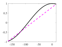
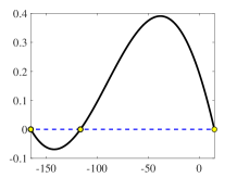
(a) $-165^{\circ}\leq\theta_{lm}-\delta_{lm}-\psi_{l}\leq 15^{\circ}$

$\cos(\theta_{lm}-\delta_{lm}-\psi_{l})$	$F(\theta_{lm},\delta_{lm},\psi_{l})$

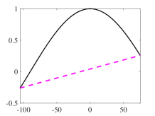
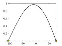
(b) $-105^{\circ}\leq\theta_{lm}-\delta_{lm}-\psi_{l}\leq 75^{\circ}$

Figure 8: The figures in the left column show visualizations of the function $\cos(\theta_{lm}-\delta_{lm}-\psi_{l})$ (black curve) and the line connecting the endpoints of this function at $\underline{\theta}_{lm}$ and $\overline{\theta}_{lm}$ (dashed magenta line) for different values of $\delta_{lm}$, $\underline{\theta}_{lm}$, and $\overline{\theta}_{lm}$. The figures in the right column show the corresponding function $F(\theta_{lm})$ and its roots between $\underline{\theta}_{lm}-\delta_{lm}-\psi_{l}$ and $\overline{\theta}_{lm}-\delta_{lm}-\psi_{l}$.

This appendix details the process of selecting appropriate tangent lines to the sine and cosine functions for arguments that take a general range of values in order to construct valid convex envelopes. While finding tangent lines for sine and cosine functions at any point is relatively straightforward — one can simply take the derivative to obtain the slope and align the line with the tangent point — the real challenge lies in identifying tangent lines that do not intersect the sine or cosine function at any other points. This occurs due to the possible variation in curvature of the sine and cosine functions for arguments within a general range of values. If the curvature’s sign does not change, tangent lines will not intersect the sine and cosine function at any other points.

The case that poses a challenge is when the curvature’s sign changes, leading to the possibility of a tangent line intersecting the function at another point. Hence, the initial step in selecting appropriate tangent lines is to examine whether the curvature’s sign changes within the specified range for the trigonometric function’s argument. To tackle this issue, we introduce an auxiliary function, denoted as $F(\theta_{lm})$ in (X), which helps us ascertain whether the curvature of the trigonometric function changes within the range $[\underline{\theta}_{lm}-\delta_{lm}-\psi_{l}$, $\overline{\theta}_{lm}-\delta_{lm}-\psi_{l}]$. The function $F(\theta_{lm})$ captures the difference between the trigonometric function $\cos(\theta_{lm}-\delta_{lm}-\psi_{l})$ and the straight line connecting its endpoints at $\underline{\theta}_{lm}$ and $\overline{\theta}_{lm}$:

$$F(\theta_{lm})=\cos(\theta_{lm}-\delta_{lm}-\psi_{l})-\cos(\overline{\theta}_{lm}-\delta_{lm}-\psi_{l})$$

$$\qquad\quad-\frac{\cos(\overline{\theta}_{lm}-\delta_{lm}-\psi_{l})-\cos(\underline{\theta}_{lm}-\delta_{lm}-\psi_{l})}{\overline{\theta}_{lm}-\underline{\theta}_{lm}}$$

$$\qquad\quad\times\left(\theta_{lm}-\overline{\theta}_{lm}-\psi_{l}\right).$$ (16)

The set of zeros of the derivative of $F(\theta_{lm})$, i.e., the set of solutions to $\frac{dF(\theta_{lm})}{d\theta_{lm}}=0$, is a key quantity when determining if the curvature of $\cos(\theta_{lm}-\delta_{lm}-\psi_{l})$ changes between $\underline{\theta}_{lm}-\delta_{lm}-\psi_{l}$ and $\overline{\theta}_{lm}-\delta_{lm}-\psi_{l}$. In Fig. 8, on the left side, we present illustrative examples of the function $\cos(\theta_{lm}-\delta_{lm}-\psi_{l})$ (depicted by the black curve) along with the dashed magenta line representing the connection between its endpoints at $\underline{\theta}_{lm}-\delta_{lm}-\psi_{l}$ and $\overline{\theta}_{lm}-\delta_{lm}-\psi_{l}$. The right side visualizes the function $F(\theta_{lm})$ itself, with its roots indicated by yellow circles.

The derivative of $F(\theta_{lm})$ is

$$\frac{dF(\theta_{lm})}{d\theta_{lm}}=-\sin(\theta_{lm}-\delta_{lm}-\psi_{l})$$

$$\quad-\frac{\cos(\overline{\theta}_{lm}-\delta_{lm}-\psi_{l})-\cos(\underline{\theta}_{lm}-\delta_{lm}-\psi_{l})}{\overline{\theta}_{lm}-\underline{\theta}_{lm}}.$$ (17)

We denote the set of zeroes for $\frac{dF(\theta_{lm})}{d\theta_{lm}}=0$ by $\mathcal{Z}_{\underline{\theta}_{lm},\overline{\theta}_{lm},\delta_{lm},\psi_{l}}$, where the subscripts indicate that the set is parameterized by $\underline{\theta}_{lm}$, $\overline{\theta}_{lm}$, $\delta_{lm}$, and $\psi_{l}$:

$$\mathcal{Z}_{\underline{\theta}_{lm},\overline{\theta}_{lm},\delta_{lm},\psi_{l}}=$$

$$\Big{\{}(-1)^{\kappa}\arcsin\left(\frac{\cos(\underline{\theta}_{lm}-\delta_{lm})-\cos(\overline{\theta}_{lm}-\delta_{lm})}{\left(\overline{\theta}_{lm}-\underline{\theta}_{lm}\right)}\right)+\pi\kappa,$$

$$\qquad\kappa=\ldots,-3,-2,-1,0,1,2,3,\ldots\Big{\}}.$$ (18)

Let $\left|\,\cdot\,\right|$ denote the cardinality of a set. The cardinality of $\mathcal{Z}_{\underline{\theta}_{lm},\overline{\theta}_{lm},\delta_{lm},\psi_{l}}$ determines whether the tangent lines to the trigonometric function at different points within $\underline{\theta}_{lm}-\delta_{lm}-\psi_{l}$ and $\overline{\theta}_{lm}-\delta_{lm}-\psi_{l}$ have multiple intersections with the trigonometric function. If $\mathcal{Z}_{\underline{\theta}_{lm},\overline{\theta}_{lm},\delta_{lm},\psi_{l}}$ is empty, it indicates that the curvature of the trigonometric function does not change. Thus, no tangent lines will have another intersection with the function. In this case, the slopes of the $k^{th}$ tangent line (referred to as $m_{k}$) at an arbitrary point within the interval, $(\phi_{lm},\cos(\phi_{lm}-\delta_{lm}-\psi_{l})$, is the derivative of the trigonometric function at this point $\left(m_{k}=\frac{d(\cos(\theta_{lm}-\delta_{lm}-\psi_{l}))}{d\theta_{lm}}|_{\phi_{lm}}=-\sin(\phi_{lm}-\delta_{lm}-\psi_{l})\right)$. The coordinate of the point itself gives us the offset, represented as $b_{int}$, of the tangent line which is equal to $\cos(\phi_{lm}-\delta_{lm}-\psi_{l})$.

Conversely, when $\left|\mathcal{Z}_{\underline{\theta}_{lm},\overline{\theta}_{lm},\delta_{lm},\psi_{l}}\right|\geq 1$, the tangent line to the cosine function at some point may intersect the cosine function again at a different point. To address this concern, we identify points, denoted as $\underline{\mathcal{R}}_{lm}$ and $\overline{\mathcal{R}}_{lm}$, at the boundaries of ranges for which tangent lines do not intersect the cosine function. $\underline{\mathcal{R}}_{lm}$ and $\overline{\mathcal{R}}_{lm}$ are shown by red and yellow stars, respectively, in Fig. 4. Note that the voltage angle difference restriction, i.e., ${-}90^{\circ}\leq\theta_{lm}\leq 90^{\circ}$, guarantees that the sine and cosine functions experience at most one curvature sign change. Consequently, selecting tangent lines to the cosine function in the ranges $[\underline{\theta}_{lm}-\delta_{lm}-\psi_{l},\underline{\mathcal{R}}_{lm}]$ and $[\overline{\mathcal{R}}_{lm},\overline{\theta}_{lm}-\delta_{lm}-\psi_{l}$] is a straightforward process since the curvature of the cosine function remains consistent, with the same sign, within these ranges. This method yields linear envelopes that provide a close outer approximation to the cosine function. The technique is applicable to any angle difference range, irrespective of the trigonometric function’s curvature. Next, we will elaborate on the computation process for $\underline{\mathcal{R}}_{lm}$ and $\overline{\mathcal{R}}_{lm}$.

To determine $\underline{\mathcal{R}}_{lm}$ and $\overline{\mathcal{R}}_{lm}$ for the cosine function, we start by formulating the tangent lines to the cosine function that pass through the endpoints $\overline{\theta}_{lm}-\delta_{lm}-\psi_{l}$ and $\underline{\theta}_{lm}-\delta_{lm}-\psi_{l}$, respectively. The tangent line to the cosine function that pass through the point $\overline{\theta}_{lm}-\delta_{lm}-\psi_{l}$ is given by $\underline{F}_{tang}(\theta_{lm})$:

$$\underline{F}_{tang}(\theta_{lm})=-\sin(\theta_{lm}-\delta_{lm}-\psi_{l})(\theta_{lm}-\overline{\theta}_{lm})$$

$$\qquad\qquad\qquad+\cos(\overline{\theta}_{lm}-\delta_{lm}-\psi_{l}).$$ (19)

We subsequently define an auxiliary function, denoted as $\underline{G}(\theta_{lm})$, which represents the difference between $\underline{F}_{tang}(\theta_{lm})$ and $\cos(\theta_{lm}-\delta_{lm}-\psi_{l})$:

$$\underline{G}(\theta_{lm})=\sin(\theta_{lm}-\delta_{lm}-\psi_{l})(\theta_{lm}-\overline{\theta}_{lm})$$

$$\qquad-\cos(\overline{\theta}_{lm}-\delta_{lm}-\psi_{l})+\cos(\theta_{lm}-\delta_{lm}-\psi_{l}).$$ (20)

The root of the derivative of $\underline{G}(\theta_{lm})$, i.e., the solution to $\frac{d\underline{G}(\theta_{lm})}{d\theta_{lm}}=0$, within the interval between $\underline{\theta}_{lm}-\delta_{lm}-\psi_{l}$ and $\overline{\theta}_{lm}-\delta_{lm}-\psi_{l}$ corresponds to the value of $\underline{\mathcal{R}}_{lm}$.

Similarly, to find $\overline{\mathcal{R}}_{lm}$, we first formulate the tangent line to the cosine function that pass through the point $\underline{\theta}_{lm}-\delta_{lm}-\psi_{l}$:

$$\overline{F}_{tang}(\theta_{lm})=-\sin(\theta_{lm}-\delta_{lm}-\psi_{l})(\theta_{lm}-\underline{\theta}_{lm})$$

$$\qquad\qquad\qquad+\cos(\underline{\theta}_{lm}-\delta_{lm}-\psi_{l}).$$ (21)

Next, we define an auxiliary function, denoted as $\overline{G}(\theta_{lm})$, which represents the difference between $\overline{F}_{tang}(\theta_{lm})$ and $\cos(\theta_{lm}-\delta_{lm}-\psi_{l})$:

$$\overline{G}(\theta_{lm})=\sin(\theta_{lm}-\delta_{lm}-\psi_{l})(\theta_{lm}-\underline{\theta}_{lm})$$

$$\qquad-\cos(\underline{\theta}_{lm}-\delta_{lm}-\psi_{l})+\cos(\theta_{lm}-\delta_{lm}-\psi_{l}).$$ (22)

Analogously to the discussion above, the root of the derivative of $\overline{G}(\theta_{lm})$, i.e., the solution to $\frac{d\overline{G}(\theta_{lm})}{d\theta_{lm}}=0$, within the interval between $\underline{\theta}_{lm}-\delta_{lm}-\psi_{l}$ and $\overline{\theta}_{lm}-\delta_{lm}-\psi_{l}$, corresponds to the value of $\overline{\mathcal{R}}_{lm}$.

To locate the roots $\frac{d\underline{G}(\theta_{lm})}{d\theta_{lm}}=0$ and $\frac{d\overline{G}(\theta_{lm})}{d\theta_{lm}}=0$ within the interval $\left[\underline{\theta}_{lm}-\delta_{lm}-\psi_{l},\overline{\theta}_{lm}-\delta_{lm}-\psi_{l}\right]$, we start by applying a bisection method to obtain a close initialization for a locally convergent Newton method to determine the precise values of the roots. The reason for employing the bisection method initially is that the Newton method may converge to solutions beyond the interval of interest for periodic functions like $\frac{d\underline{G}(\theta_{lm})}{d\theta_{lm}}$ and $\frac{d\overline{G}(\theta_{lm})}{d\theta_{lm}}$. The bisection method finds approximate solutions within the interval of interest that are refined with a Newton method. The slope of tangent line to the cosine function at $\underline{\mathcal{R}}_{lm}$ (referred to as $m_{k,\underline{\mathcal{R}}_{lm}}$), is the derivative of the cosine functions at the corresponding argument for $\underline{\mathcal{R}}_{lm}$, i.e., $\left(m_{k,\underline{\mathcal{R}}_{lm}}=-\sin(\phi_{lm,\underline{\mathcal{R}}_{lm}}-\delta_{lm}-\psi_{l})\right)$. The coordinate of the point itself gives us the offset, represented as $b_{int,\underline{\mathcal{R}}_{lm}}$, of the tangent line which is equal to $\cos(\phi_{lm,\underline{\mathcal{R}}_{lm}}-\delta_{lm}-\psi_{l})$. The slope and offset for $\overline{\mathcal{R}}_{lm}$ is computed similarly.

1 function Find_Tangent($\overline{\theta}_{lm}$,$\underline{\theta}_{lm}$,$\delta_{lm}$,$\psi_{l}$,$N_{tan}$)

2      $U\leftarrow\overline{\theta}_{lm}-\delta_{lm}-\psi_{l}$, $L\leftarrow\underline{\theta}_{lm}-\delta_{lm}-\psi_{l}$.

3      Define $F(\theta_{lm})$ and $\frac{dF(\theta_{lm})}{d\theta_{lm}}$.

4      $\mathcal{Z}_{\underline{\theta}_{lm},\overline{\theta}_{lm},\delta_{lm},\psi_{l}}\leftarrow$ Find the roots of $\frac{dF(\theta_{lm})}{d\theta_{lm}}$ within $[L,U]$.

5     if $\left|\mathcal{Z}_{\underline{\theta}_{lm},\overline{\theta}_{lm},\delta_{lm},\psi_{l}}\right|<1$ then

6           At $N_{tan}$ equally spaced points within $[L,U]$:

7           for $i=1:N_{tan}$ do

8                $m_{k,i}=-\sin(\phi_{lm,i}-\delta_{lm}-\psi_{l})$ $b_{int,i}=\cos(\phi_{lm,i}-\delta_{lm}-\psi_{l})$

9                end for

10               

11                else if $\left|\mathcal{Z}_{\underline{\theta}_{lm},\overline{\theta}_{lm},\delta_{lm},\psi_{l}}\right|\geq 1$ then

12                     $\underline{\mathcal{R}}_{lm}\leftarrow\frac{dG(\theta_{lm},U)}{d\theta_{lm}}=0$

13                     $\overline{\mathcal{R}}_{lm}\leftarrow\frac{dG(\theta_{lm},L)}{d\theta_{lm}}=0$

14                     Find the tangent lines to $\cos(\theta_{lm}-\delta_{lm}-\psi_{l})$ at $\underline{\mathcal{R}}_{lm}$ and $\overline{\mathcal{R}}_{lm}$:

15                    $m_{k,\underline{\mathcal{R}}_{lm}}=-\sin(\phi_{lm,\underline{\mathcal{R}}_{lm}}-\delta_{lm}-\psi_{l})$

16                     $b_{int,\underline{\mathcal{R}}_{lm}}=\cos(\phi_{lm,\underline{\mathcal{R}}_{lm}}-\delta_{lm}-\psi_{l})$

17                    

18                    $m_{k,\overline{\mathcal{R}}_{lm}}=-\sin(\phi_{lm,\overline{\mathcal{R}}_{lm}}-\delta_{lm}-\psi_{l})$

19                     $b_{int,\overline{\mathcal{R}}_{lm}}=\cos(\phi_{lm,\overline{\mathcal{R}}_{lm}}-\delta_{lm}-\psi_{l})$

20                    

21                    Equally divide the ranges $[\overline{\mathcal{R}}_{lm},U]$ and $[L,\underline{\mathcal{R}}_{lm}]$ into $N_{tan}$ segments

22                    for $i=1:N_{tan}$ do

23                          $m_{k,i}=-\sin(\phi_{lm,i}-\delta_{lm}-\psi_{l})$ $b_{int,i}=\cos(\phi_{lm,i}-\delta_{lm}-\psi_{l})$

24                          end for

25                         

26                          end if

27                         return $m_{k}$ and $b_{int}$

28                         

Algorithm 2 Finding tangent lines

After computing $\underline{\mathcal{R}}_{lm}$ and $\overline{\mathcal{R}}_{lm}$, we select equally spaced tangent lines to the cosine function within the intervals $\left[\underline{\theta}_{lm}-\delta_{lm}-\psi_{l},\underline{\mathcal{R}}_{lm}\right]$ and $\left[\overline{\mathcal{R}}_{lm},\overline{\theta}_{lm}-\delta_{lm}-\psi_{l}\right]$.

Algorithm 2 outlines the procedure for computing these convex envelopes using carefully selected tangent lines. For notational convenience, define $L=\underline{\theta}_{lm}-\delta_{lm}-\psi_{l}$ and $U=\overline{\theta}_{lm}-\delta_{lm}-\psi_{l}$. Equations (23) and (24) define the tangent lines which form the lower and upper bounds, respectively, of the cosine envelope:

If curvature changes within $$[L,U]$$ from positive to negative:

$$\underline{L}_{\cos,i}\!\!=\!\!\begin{cases}m_{k,i}(x-\!x_{0,i})+b_{int,i},\leavevmode\nobreak\ i=1,\ldots,N_{tan},\leavevmode\nobreak\ \text{if\leavevmode\nobreak\ }x\in[L,\underline{\mathcal{R}}_{lm}]\\ m_{k,\underline{\mathcal{R}}_{lm}}(x-x_{0,\underline{\mathcal{R}}_{lm}})+b_{int,\underline{\mathcal{R}}_{lm}}\leavevmode\nobreak\ \text{if\leavevmode\nobreak\ }x\in[\underline{\mathcal{R}}_{lm},U]\end{cases}$$ (23a)

If curvature changes within $$[L,U]$$ from negative to positive:

$$\underline{L}_{\cos,i}\!\!=\!\!\begin{cases}m_{k,i}(x-\!x_{0,i})+b_{int,i},\leavevmode\nobreak\ i=1,\ldots,N_{tan},\leavevmode\nobreak\ \text{if\leavevmode\nobreak\ }x\in[\overline{\mathcal{R}}_{lm},U]\\ m_{k,\underline{\mathcal{R}}_{lm}}(x-x_{0,\underline{\mathcal{R}}_{lm}})+b_{int,\underline{\mathcal{R}}_{lm}}\leavevmode\nobreak\ \text{if\leavevmode\nobreak\ }x\in[L,\overline{\mathcal{R}}_{lm}]\end{cases}$$ (23b)

If curvature does not change within $$[L,U]$$ and it is negative:

$$\underline{L}_{\cos,i}\!\!=\!\!\begin{cases}\frac{\cos(U)-\cos(L)}{U-L}(x-L)+\cos(L)\leavevmode\nobreak\ \leavevmode\nobreak\ \leavevmode\nobreak\ \leavevmode\nobreak\ \leavevmode\nobreak\ \forall x\in[L,U],\end{cases}$$ (23c)

If curvature does not change within $$[L,U]$$ and is positive:

$$\underline{L}_{\cos,i}\!\!=\!\!\begin{cases}\frac{\cos(U)-\cos(L)}{U-L}(x-L)+\cos(L)\leavevmode\nobreak\ \leavevmode\nobreak\ \leavevmode\nobreak\ \leavevmode\nobreak\ \leavevmode\nobreak\ \forall x\in[L,U]\end{cases}$$ (23d)

Similarly, the upper bound for the cosine envelope is:

If curvature changes within $$[L,U]$$ from positive to negative:

$$\overline{L}_{\cos,i}\!\!=\!\!\begin{cases}m_{k,i}(x-\!x_{0,i})+b_{int,i},\leavevmode\nobreak\ i\!=\!1,\ldots,N_{tan},\leavevmode\nobreak\ \text{if\leavevmode\nobreak\ }x\in[\overline{\mathcal{R}}_{lm},U]\\ m_{k,\overline{\mathcal{R}}_{lm}}(x-x_{0,\overline{\mathcal{R}}_{lm}})+b_{int,\overline{\mathcal{R}}_{lm}}\leavevmode\nobreak\ \text{if\leavevmode\nobreak\ }x\in[L,\overline{\mathcal{R}}_{lm}]\end{cases}$$ (24a)

If curvature changes within $$[L,U]$$ from negative to positive:

$$\overline{L}_{\cos,i}\!\!=\!\!\begin{cases}m_{k,i}(x-\!x_{0,i})+b_{int,i},\leavevmode\nobreak\ i\!=\!1,\ldots,N_{tan},\leavevmode\nobreak\ \text{if\leavevmode\nobreak\ }x\in[L,\underline{\mathcal{R}}_{lm}]\\ m_{k,\underline{\mathcal{R}}_{lm}}(x-x_{0,\underline{\mathcal{R}}_{lm}})+b_{int,\underline{\mathcal{R}}_{lm}}\leavevmode\nobreak\ \text{if\leavevmode\nobreak\ }x\in[\underline{\mathcal{R}}_{lm},U]\end{cases}$$ (24b)

If curvature does not change within $$[L,U]$$ and is negative:

$$\overline{L}_{\cos,i}\!\!=\!\!\begin{cases}\frac{\cos(U)-\cos(L)}{U-L}(x-L)+\cos(L)\leavevmode\nobreak\ \leavevmode\nobreak\ \leavevmode\nobreak\ \leavevmode\nobreak\ \leavevmode\nobreak\ \forall x\in[L,U]\end{cases}$$ (24c)

If curvature does not change within $$[L,U]$$ and is positive:

$$\overline{L}_{\cos,i}\!\!=\!\!\begin{cases}\frac{\cos(U)-\cos(L)}{U-L}(x-L)+\cos(L)\leavevmode\nobreak\ \leavevmode\nobreak\ \leavevmode\nobreak\ \leavevmode\nobreak\ \leavevmode\nobreak\ \forall x\in[L,U]\end{cases}$$ (24d)

where $\overline{L}_{\cos,i}$ and $\underline{L}_{\cos,i}$ are the $i^{th}$ tangent lines which upper and lower bound, respectively, the cosine function; $x$ equals $\theta_{lm}-\delta_{lm}-\psi_{l}$; $x_{0,i}$, $x_{0,\underline{\mathcal{R}}_{lm}}$, and $x_{0,\overline{\mathcal{R}}_{lm}}$ represent the horizontal coordinates of the corresponding points within their respective intervals; $b_{int,i}$, $b_{int,\underline{\mathcal{R}}_{lm}}$, and $b_{int,\overline{\mathcal{R}}_{lm}}$ denote the vertical coordinates of these same points, which determines the offset for the tangent lines; and $m_{k,i}$, $m_{k,\underline{\mathcal{R}}_{lm}}$, and $m_{k,\overline{\mathcal{R}}_{lm}}$ signify the slopes of the tangent lines at these points. Note that when the curvature of the trigonometric function does not change within an interval, either the lower or upper envelope can be defined as a line connecting both ends of the trigonometric function. For instance, consider a specific angle $\left(\phi_{lm}-\delta_{lm}-\psi_{l}\right)$ within the interval $[L,\underline{\mathcal{R}}_{lm}]$. In this case, $m_{k,i}$ is equal to ${-}\sin\left(\phi_{lm}-\delta_{lm}-\psi_{l}\right)$, which represents the first derivative of the cosine function at $x_{0,i}=\phi_{lm}-\delta_{lm}-\psi_{l}$. The corresponding offset for this point is $b_{int,i}=\cos\left(\phi_{lm}-\delta_{lm}-\psi_{l}\right)$. Tangent lines for the lower and upper bounds of the sine function are formulated similarly.

Equation (13) formulates the cosine function. To complete the full exposition, we similarly formulate the lower and upper envelopes for the sine function by defining a function $H(\theta_{lm})$. Here, the function $H(\theta_{lm})$ represents the difference between the trigonometric function $\sin(\theta_{lm}-\delta_{lm}-\psi_{l})$ itself and the line which connects the endpoints of $\sin(\theta_{lm}-\delta_{lm}-\psi_{l})$ at $\underline{\theta}_{lm}$ and $\overline{\theta}_{lm}$:

$$H(\theta_{lm})=\sin(\theta_{lm}-\delta_{lm}-\psi_{l})-\sin(\overline{\theta}_{lm}-\delta_{lm}-\psi_{l})$$

$$\qquad\quad-\frac{\sin(\overline{\theta}_{lm}-\delta_{lm}-\psi_{l})-\sin(\underline{\theta}_{lm}-\delta_{lm}-\psi_{l})}{\overline{\theta}_{lm}-\underline{\theta}_{lm}}$$

$$\qquad\quad\times\left(\theta_{lm}-\overline{\theta}_{lm}-\psi_{l}\right).$$ (25)

The number of zeros of the first derivative of $H(\theta_{lm})$, i.e., the number of solutions for $\frac{dH(\theta_{lm})}{d\theta_{lm}}=0$, is a key quantity to determine if the curvature of $\sin(\theta_{lm}-\delta_{lm}-\psi_{l})$ changes between $\underline{\theta}_{lm}-\delta_{lm}-\psi_{l}$ and $\overline{\theta}_{lm}-\delta_{lm}-\psi_{l}$. If $\frac{dH(\theta_{lm})}{d\theta_{lm}}=0$ has no solutions, then the curvature of the $\sin(\theta_{lm}-\delta_{lm}-\psi_{l})$ does not change between $\underline{\theta}_{lm}-\delta_{lm}-\psi_{l}$ and $\overline{\theta}_{lm}-\delta_{lm}-\psi_{l}$. Our proposed QC relaxation uses envelopes $\left\langle\sin(\theta_{lm}-\delta_{lm}-\psi_{l})\right\rangle^{S^{\prime}}$ formed by combining the tangent lines. Depending upon the sign of the sine function’s curvature and the number of solutions to $\frac{dH(\theta_{lm})}{d\theta_{lm}}=0$, there are different upper and lower bounds on the sine function’s envelopes:

If $$\frac{dH(\theta_{lm})}{d\theta_{lm}}=0$$ has one or more solutions:

$$\left\langle\sin(\theta_{lm}-\delta_{lm}-\psi_{l})\right\rangle^{S^{\prime}}=\begin{cases}\!\widecheck{S}^{\prime}\!:\begin{cases}\widecheck{S}^{\prime}\!\leq\overline{L}_{\sin,i},\leavevmode\nobreak\ i=1,\ldots,N_{tan}\\ \widecheck{S}^{\prime}\!\geq\underline{L}_{\sin,i},\leavevmode\nobreak\ i=1,\ldots,N_{tan}\end{cases}\end{cases}$$ (26a)

If $$\frac{dH(\theta_{lm})}{d\theta_{lm}}=0$$ has no solutions & curvature sign is negative:

$$\left\langle\sin(\theta_{lm}-\delta_{lm}-\psi_{l})\right\rangle^{S^{\prime}}=\begin{cases}\!\widecheck{S}^{\prime}\!:\begin{cases}\widecheck{S}^{\prime}\!\leq\overline{L}_{\sin,i},\leavevmode\nobreak\ i=1,\ldots,N_{tan}\\ \widecheck{S}^{\prime}\!\geq\underline{L}_{\sin,i},\leavevmode\nobreak\ i=1\end{cases}\end{cases}$$ (26b)

If $$\frac{dH(\theta_{lm})}{d\theta_{lm}}=0$$ has no solutions & curvature sign is positive:

$$\left\langle\sin(\theta_{lm}-\delta_{lm}-\psi_{l})\right\rangle^{S^{\prime}}=\begin{cases}\!\widecheck{S}^{\prime}\!:\begin{cases}\widecheck{S}^{\prime}\!\leq\overline{L}_{\sin,i},\leavevmode\nobreak\ i=1\\ \widecheck{S}^{\prime}\!\geq\underline{L}_{\sin,i},\leavevmode\nobreak\ i=1,\ldots,N_{tan}\end{cases}\end{cases}$$ (26c)

where $\overline{L}_{\sin,i}$ and $\underline{L}_{\sin,i}$ are the $i^{th}$ tangent lines which upper and lower bound, respectively, the sine function.

Equations (27) and (28) mathematically represent the tangent lines for the lower and upper bounds of the sine function, respectively:

If curvature changes within $$[L,U]$$ from positive to negative:

$$\underline{L}_{\sin,i}\!\!=\!\!\begin{cases}m_{k,i}(x-\!x_{0,i})+b_{int,i},\leavevmode\nobreak\ i=1,\ldots,N_{tan},\leavevmode\nobreak\ \leavevmode\nobreak\ \text{if\leavevmode\nobreak\ }x\in[L,\underline{\mathcal{R}}_{lm}]\\ m_{k,\underline{\mathcal{R}}_{lm}}(x-x_{0,\underline{\mathcal{R}}_{lm}})+b_{int,\underline{\mathcal{R}}_{lm}}\leavevmode\nobreak\ \text{if\leavevmode\nobreak\ }x\in[\underline{\mathcal{R}}_{lm},U]\end{cases}$$ (27a)

If curvature changes within $$[L,U]$$ from negative to positive:

$$\underline{L}_{\sin,i}\!\!=\!\!\begin{cases}m_{k,i}(x-\!x_{0,i})+b_{int,i},\leavevmode\nobreak\ i=1,\ldots,N_{tan},\leavevmode\nobreak\ \text{if\leavevmode\nobreak\ }x\in[\overline{\mathcal{R}}_{lm},U]\\ m_{k,\underline{\mathcal{R}}_{lm}}(x-x_{0,\underline{\mathcal{R}}_{lm}})+b_{int,\underline{\mathcal{R}}_{lm}}\leavevmode\nobreak\ \text{if\leavevmode\nobreak\ }x\in[L,\overline{\mathcal{R}}_{lm}]\end{cases}$$ (27b)

If curvature does not change within $$[L,U]$$ and is negative:

$$\underline{L}_{\sin,i}\!\!=\!\!\begin{cases}\frac{\sin(U)-\sin(L)}{U-L}(x-L)+\sin(L)\leavevmode\nobreak\ \leavevmode\nobreak\ \leavevmode\nobreak\ \leavevmode\nobreak\ \leavevmode\nobreak\ \forall x\in[L,U],\end{cases}$$ (27c)

If curvature does not change within $$[L,U]$$ and is positive:

$$\underline{L}_{\sin,i}\!\!=\!\!\begin{cases}\frac{\sin(U)-\sin(L)}{U-L}(x-L)+\sin(L)\leavevmode\nobreak\ \leavevmode\nobreak\ \leavevmode\nobreak\ \leavevmode\nobreak\ \leavevmode\nobreak\ \forall x\in[L,U]\end{cases}$$ (27d)

Similarly, the upper bound for the sine function can be represented as follows:

If curvature changes within $$[L,U]$$ from positive to negative:

$$\overline{L}_{\sin,i}\!\!=\!\!\begin{cases}m_{k,i}(x-\!x_{0,i})+b_{int,i},\leavevmode\nobreak\ i=1,\ldots,N_{tan},\leavevmode\nobreak\ \text{if\leavevmode\nobreak\ }x\in[\overline{\mathcal{R}}_{lm},U]\\ m_{k,\overline{\mathcal{R}}_{lm}}(x-x_{0,\overline{\mathcal{R}}_{lm}})+b_{int,\overline{\mathcal{R}}_{lm}}\leavevmode\nobreak\ \text{if\leavevmode\nobreak\ }x\in[L,\overline{\mathcal{R}}_{lm}]\end{cases}$$ (28a)

If curvature changes within $$[L,U]$$ from negative to positive:

$$\overline{L}_{\sin,i}\!\!=\!\!\begin{cases}m_{k,i}(x-\!x_{0,i})+b_{int,i},\leavevmode\nobreak\ i=1,\ldots,N_{tan},\leavevmode\nobreak\ \text{if\leavevmode\nobreak\ }x\in[L,\underline{\mathcal{R}}_{lm}]\\ m_{k,\underline{\mathcal{R}}_{lm}}(x-x_{0,\underline{\mathcal{R}}_{lm}})+b_{int,\underline{\mathcal{R}}_{lm}}\leavevmode\nobreak\ \text{if\leavevmode\nobreak\ }x\in[\underline{\mathcal{R}}_{lm},U]\end{cases}$$ (28b)

If curvature does not change within $$[L,U]$$ and is negative:

$$\overline{L}_{\sin,i}\!\!=\!\!\begin{cases}\frac{\sin(U)-\sin(L)}{U-L}(x-L)+\sin(L)\leavevmode\nobreak\ \leavevmode\nobreak\ \leavevmode\nobreak\ \leavevmode\nobreak\ \leavevmode\nobreak\ \forall x\in[L,U]\end{cases}$$ (28c)

If curvature does not change within $$[L,U]$$ and is positive:

$$\overline{L}_{\sin,i}\!\!=\!\!\begin{cases}\frac{\sin(U)-\sin(L)}{U-L}(x-L)+\sin(L)\leavevmode\nobreak\ \leavevmode\nobreak\ \leavevmode\nobreak\ \leavevmode\nobreak\ \leavevmode\nobreak\ \forall x\in[L,U]\end{cases}$$ (28d)

where $x$ equals $\theta_{lm}-\delta_{lm}-\psi_{l}$; $x_{0,i}$, $x_{0,\underline{\mathcal{R}}_{lm}}$, and $x_{0,\overline{\mathcal{R}}_{lm}}$ represent the horizontal coordinates of the corresponding points within their respective intervals; $b_{int,i}$, $b_{int,\underline{\mathcal{R}}_{lm}}$, and $b_{int,\overline{\mathcal{R}}_{lm}}$ denote the vertical coordinates of these points within their corresponding intervals, determining the offset for the tangent lines; and $m_{k,i}$, $m_{k,\underline{\mathcal{R}}_{lm}}$, and $m_{k,\overline{\mathcal{R}}_{lm}}$ signify the slopes of the tangent lines at specific points within their respective intervals.

References

- [1] W. Bukhsh, A. Grothey, K. McKinnon, and P. Trodden, “Local Solutions of the Optimal Power Flow Problem,” IEEE Trans. Power Syst., vol. 28, no. 4, pp. 4780–4788, 2013.
- [2] D. Bienstock and A. Verma, “Strong NP-Hardness of AC Power Flows Feasibility,” Oper. Res. Lett., vol. 47, no. 6, pp. 494–501, 2019.
- [3] J. Carpentier, “Contribution to the Economic Dispatch Problem,” Bull. Soc. Franc. Elect, vol. 8, no. 3, pp. 431–447, 1962.
- [4] J. Momoh, R. Adapa, and M. El-Hawary, “A Review of Selected Optimal Power Flow Literature to 1993. Parts I and II,” IEEE Trans. Power Syst., vol. 14, no. 1, pp. 96–111, Feb. 1999.
- [5] A. Castillo and R. O’Neill, “Survey of Approaches to Solving the ACOPF (OPF Paper 4),” FERC, Tech. Rep., Mar. 2013.
- [6] M. Lu, H. Nagarajan, R. Bent, S. D. Eksioglu, and S. J. Mason, “Tight Piecewise Convex Relaxations for Global Optimization of Optimal Power Flow,” in Power Syst. Comput. Conf. (PSCC), Dublin, Ireland, June 2018.
- [7] D. K. Molzahn and L. A. Roald, “AC Optimal Power Flow with Robust Feasibility Guarantees,” in Power Syst. Comput. Conf. (PSCC), Dublin, Ireland, June 2018.
- [8] A. Lorca and X. A. Sun, “The Adaptive Robust Multi-Period Alternating Current Optimal Power Flow Problem,” IEEE Trans. Power Syst., vol. 33, no. 2, pp. 1993–2003, March 2018.
- [9] D. K. Molzahn, B. C. Lesieutre, and C. L. DeMarco, “A Sufficient Condition for Power Flow Insolvability With Applications to Voltage Stability Margins,” IEEE Trans. Power Syst., vol. 28, no. 3, pp. 2592–2601, Aug. 2013.
- [10] D. K. Molzahn, “Computing the Feasible Spaces of Optimal Power Flow Problems,” IEEE Trans. Power Syst., vol. 32, no. 6, pp. 4752–4763, Nov. 2017.
- [11] M. R. Narimani, D. K. Molzahn, D. Wu, and M. L. Crow, “Empirical Investigation of Non-Convexities in Optimal Power Flow Problems,” in American Control Conf. (ACC), Milwaukee, WI, USA, June 2018, pp. 3847–3854.
- [12] B. Kocuk, S. S. Dey, and X. A. Sun, “New Formulation and Strong MISOCP Relaxations for AC Optimal Transmission Switching Problem,” IEEE Trans. Power Syst., vol. 32, no. 6, pp. 4161–4170, 2017.
- [13] D. K. Molzahn and I. A. Hiskens, “A Survey of Relaxations and Approximations of the Power Flow Equations,” Found. Trends Electric Energy Syst., vol. 4, no. 1-2, pp. 1–221, Feb. 2019.
- [14] C. Coffrin, H. Hijazi, and P. Van Hentenryck, “The QC Relaxation: A Theoretical and Computational Study on Optimal Power Flow,” IEEE Trans. Power Syst., vol. 31, no. 4, pp. 3008–3018, July 2016.
- [15] C. Coffrin, H. L. Hijazi, and P. Van Hentenryck, “Strengthening the SDP Relaxation of AC Power Flows with Convex Envelopes, Bound Tightening, and Valid Inequalities,” IEEE Trans. Power Syst., vol. 32, no. 5, pp. 3549–3558, Sept. 2017.
- [16] K. Bestuzheva, H. Hijazi, and C. Coffrin, “Convex Relaxations for Quadratic On/Off Constraints and Applications to Optimal Transmission Switching,” INFORMS J. Comput., vol. 32, no. 3, pp. 682–696, 2020.
- [17] C. Chen, A. Atamtürk, and S. S. Oren, “A Spatial Branch-and-Cut Algorithm for Nonconvex QCQP with Bounded Complex Variables,” Math. Prog., vol. 165, pp. 549–577, 2017.
- [18] M. R. Narimani, D. K. Molzahn, and M. L. Crow, “Improving QC Relaxations of OPF Problems via Voltage Magnitude Difference Constraints and Envelopes for Trilinear Monomials,” in 20th Power Syst. Comput. Conf. (PSCC), Dublin, Ireland, June 2018.
- [19] M. R. Narimani, D. K. Molzahn, H. Nagarajan, and M. L. Crow, “Comparison of Various Trilinear Monomial Envelopes for Convex Relaxations of Optimal Power Flow Problems,” in IEEE Global Conf. Signal Infor. Proc. (GlobalSIP), Anaheim, CA, USA, November 2018, pp. 865–869.
- [20] B. Kocuk, S. S. Dey, and X. A. Sun, “Strong SOCP Relaxations for the Optimal Power Flow Problem,” Oper. Res., vol. 64, no. 6, pp. 1177–1196, May 2016.
- [21] ——, “Matrix Minor Reformulation and SOCP-based Spatial Branch-and-Cut Method for the AC Optimal Power Flow Problem,” Math. Prog. Comput., vol. 10, no. 4, pp. 557–596, 2018.
- [22] M. Narimani, D. Molzahn, and M. Crow, “Tightening QC Relaxations of AC Optimal Power Flow Problems via Complex Per Unit Normalization,” arXiv:1912.05061v2, May. 2020.
- [23] M. R. Narimani, Strengthening QC Relaxations of Optimal power Flow Problems by Exploiting Various Coordinate Changes. Missouri University of Science and Technology, 2020.
- [24] K. Sundar, H. Nagarajan, S. Misra, M. Lu, C. Coffrin, and R. Bent, “Optimization-Based Bound Tightening using a Strengthened QC-Relaxation of the Optimal Power Flow Problem,” arXiv:1809.04565, Sept. 2018.
- [25] M. Farivar, C. R. Clarke, S. H. Low, and K. M. Chandy, “Inverter VAR Control for Distribution Systems with Renewables,” in IEEE Int. Conf. Smart Grid Comm. (SmartGridComm), Brussels, Belgium, Oct. 2011, pp. 457–462.
- [26] A. D. Rikun, “A Convex Envelope Formula for Multilinear Functions,” J. Global Optimiz., vol. 10, no. 4, pp. 425–437, 1997.
- [27] K. Sundar, S. Sanjeevi, and H. Nagarajan, “Sequence of Polyhedral Relaxations for Nonlinear Univariate Functions,” Optimization and Engineering, vol. 23, no. 2, pp. 877–894, 2022.
- [28] C. Coffrin and P. Van Hentenryck, “A Linear-Programming Approximation of AC Power Flows,” INFORMS J. Comput., vol. 26, no. 4, pp. 718–734, 2014.
- [29] IEEE PES Task Force on Benchmarks for Validation of Emerging Power System Algorithms, “The Power Grid Library for Benchmarking AC Optimal Power Flow Algorithms,” arXiv:1908.02788, Aug. 2019. [Online]. Available: https://github.com/power-grid-lib/pglib-opf
- [30] I. Dunning, J. Huchette, and M. Lubin, “JuMP: A Modeling Language for Mathematical Optimization,” SIAM Rev., vol. 59, no. 2, pp. 259–320, June 2017.
- [31] C. Coffrin, R. Bent, K. Sundar, Y. Ng, and M. Lubin, “PowerModels.jl: An Open-Source Framework for Exploring Power Flow Formulations,” in Power Syst. Comput. Conf. (PSCC), Dublin, Ireland, June 2018.