Mobile Traffic Prediction at the Edge through Distributed and Transfer Learning

Abstract

Traffic prediction represents one of the crucial tasks for smartly optimizing the mobile network. The research in this topic concentrated in making predictions in a centralized fashion, i.e., by collecting data from the different network elements. This translates to a considerable amount of energy for data transmission and processing. In this work, we propose a novel prediction framework based on edge computing which uses datasets obtained on the edge through a large measurement campaign. Two main Deep Learning architectures are designed, based on Convolutional Neural Networks (CNNs) and Recurrent Neural Networks (RNNs), and tested under different training conditions. In addition, Knowledge Transfer Learning (KTL) techniques are employed to improve the performance of the models while reducing the required computational resources. Simulation results show that the CNN architectures outperform the RNNs. An estimation for the needed training energy is provided, highlighting KTL ability to reduce the energy footprint of the models of 60% and 90% for CNNs and RNNs, respectively. Finally, two cutting-edge explainable Artificial Intelligence techniques are employed to interpret the derived learning models.

Edge Computing, Energy Efficiency, Machine Learning, Mobile Traffic Prediction, Transfer Learning.

I Introduction

Traffic analysis and prediction represent crucial tasks for mobile network operators to properly and efficiently manage the network, by implementing, e.g., network planning, Quality of Experience (QoE) management, anomaly detection algorithms, cyber-security frameworks. Historically, these tasks have been performed by mobile networks operators through their data collected for billing, the Call Detail Records (CDRs). This solution relies on dedicated servers that retrieve the data from the base stations and then process it in the core part of the network. Therefore, data has to be transmitted from the edge to central servers, which implies possible privacy issues due the transmission of sensible information, higher network congestion probability and higher energy consumption, due to the massive volume of data to be exchanged.

The availability of such huge amount of data together with the evolution in computational capabilities allow to take advantage of Deep Learning (DL) to tackle multiple problems in network management. In fact, DL represents one of the pillar of the sixth generation (6G) mobile networks to address intelligent management solutions [1]. Nevertheless, there is a complexity downside that normally is not taken into account when picturing this intelligent, autonomous and DL-based technologies. In fact, the Artificial Neural Networks (ANNs) adopted in DL are made of many neurons and layers identified by a high number of trainable parameters to execute identified tasks with high accuracy. This implies an extremely high computational complexity, which requires an equally high energy consumption. For example, training a single Natural Language Processing (NLP) ML model is equivalent to 284 tons of carbon dioxide emission, i.e., five times the lifetime emissions of an medium size car [2]. Therefore, it is of paramount importance to adopt sustainable design principle for AI [3] and advocate for efficiency, as an evaluation criterion, alongside accuracy and other related measures.

Multi-access Edge Computing (MEC) represents an efficient solution to address data privacy, network congestion and energy sustainability issues [4]. In fact, the main idea behind MEC is to process data directly at the edge without sending them to central servers, possibly managed by a third party. This approach solves both privacy and congestion concerns. Moreover, it has been demonstrated that MEC can save up to $25\%$ of the network energy consumption [5]. These savings are mainly enabled by the reduced communication cost (avoiding data transmission to the central server) and the use of smaller and energy-efficient devices, which use less power for refrigerating respect to data centres.

In line with the above, we propose a distributed DL solution for traffic prediction implemented directly at the base stations. Moreover, we leverage Knowledge Transfer Learning (KTL) [6] to additionally reduce the complexity of the training phase and, consequently, the energy consumed. The main principle of KTL is to exploit the knowledge of a teacher network trained with general data, and then retrain student networks on a more specific local dataset. This allows to reduce the required computational resources by exploiting the learned knowledge of the teacher base station for the other student base stations in a collaborative and distributed fashion.

In addition, we provide insights on the DL models built for traffic prediction through Visual-based eXplainable AI (v-XAI) [7]. These tools give explanations of black-box models to reveal their behavior and underlying decision-making mechanisms with a specific focus on how to visually represent its results for a general audience. Our proposed analysis allows to better understand the output of both DL models and of the KTL process.

In this work, we use data captured from several operative base stations located in Barcelona, Spain. Data are collected with OWL [8], a tool capable of decoding the unencrypted LTE Physical Downlink Control Channel (PDCCH). Among the control data contained in the PDCCH, the Downlink Control Information (DCI) messages can be retrieved, which contain radio-link level settings for the user communication, both for the downlink and uplink channels. These information includes, among others, the Radio Network Temporary Identifier (RNTI) (a temporary ID assigned to each UE), the Modulation and Coding Scheme (MCS) and the number of allocated Resource Blocks (RBs) per frame. Therefore, we can infer the resources allocated to the users and the throughput of the base station. Our solution, being based on control data and avoiding usual deep packet inspection techniques from the user plane, reduces the memory footprint for processing and includes an additional level of privacy, since it does not need to access the user generated content.

We investigate Convolutional Neural Networks (CNNs) and Recurrent Neural Networks (RNNs) with standard stand-alone database and with the transfer paradigm. Simulation results show that the predictions in the local datasets presents good levels of accuracy. The models evaluated with the transfer paradigm have improved accuracy performance with respect to their correspondent stand-alone versions. All the results obtained are in line with benchmark solutions based on Support Vector Regression (SVR) [9] applied to the stand-alone database. In our analysis, we also detail the difficulties in applying KTL to SVR. Moreover, we measure the complexity of the proposed models together with the energy savings obtained by the adoption of KTL, which can reach up to 60% for CNN and 90% for RNN. Finally, we interpret the learned models through the XAI SmoothGrad [10] and Layer-wise Relevance Propagation (LRP) [11] algorithms. As a result, the original contributions of the paper are summarized in the following list.

• We design of a novel and efficient MEC-based framework for collecting and processing mobile data obtained by passively sniffing the LTE control channel from different base stations. We also provide an Exploratory Data Analysis (EDA) for evaluating the main characteristics of the different datasets.

• We design two prediction models based on RNNs and CNNs.

• We assess the performance of the proposed models with both stand-alone and transfer learning paradigms. We also present a comparison with SVR-based solution as benchmark.

• We analyze the complexity and the energy footprint of the proposed models.

• We discuss on the interpretation of the obtained models by applying two XAI algorithms (SmoothGrad and LRP).

The rest of the paper is organized as follows. The previous literature and the innovative aspects of this work are presented in Section II. The datasets used and the analysis of their main features are described in Section III. Section IV reports the description of the tackled tasks and of the proposed DL models and architectures. Section V contains a dissertation about the models’ training, accuracy and complexity performance together with their energy consumption. In Section VI, the outcomes of the two XAI techniques are discussed. Finally, Section VII concludes the paper with remarks and possible future directions.

II Related Work

Traffic prediction has been tackled for years due to their relevance for mobile network management. Traditional approaches involve SVR and AutoRegressive Integrated Moving Average (ARIMA) [12] [13] models. In the last years, thanks to the evolution in computational capabilities, DL methods were able to overcome the traditional Machine Learning (ML) models. This is due to DL structural ability to successfully recognize the complex patterns and relationships present in mobile traffic time series [14], and in other networking-related tasks [15] [16]. In particular, good traffic prediction results have been obtained in [17] through densely connected two-dimensional CNNs, which are able to spot both the spatial and temporal dependence of cell traffic. In [18], an autoencoder-based deep model for spatial modeling and Long Short-Term Memory units (LSTMs) for temporal modeling have been proposed and tested using a dataset provided by China Mobile. Similarly, in [19] LSTMs equipped with stochastic connectivity have been proposed with the aim of reducing the considerable computing cost of the corresponding vanilla version. Combinations of the two architectures mentioned above were effective as well, as presented in [20] [21].

However, most of the previous literature regarding traffic prediction is characterized by a centralized approach, in which data are available on dedicated servers that need to retrieve it from the edge. A step toward a MEC solution has been done in [22], where CDR has been used to train models for different neighbourhoods of the city of Milan with a Federated Learning paradigm. In addition, Model-Agnostic Meta-Learning (MAML) has been used to train a sensitive initial model that can adapt to heterogeneous scenarios in different regions. Summarizing, the majority of the cited works use CDR, i.e. mobile networks operators’ data which are used for billing purposes. This approach clearly implies possible leaks of security, as well as high amount of data to be exchanged in the network, which translates into a considerable amount of energy.

Instead, this work aims at showing the advantages of building one generic model to be trained directly on distributed sources of data (i.e., the base stations) to perform prediction, and to apply KTL from the different sites. The same datasets have been already adopted in [23] and [24], but the work in such cases concentrate on different problems (traffic classification and joint prediction and classification, respectively) and do not allow a meaningful comparison according to the scope of this work.

Finally, to the best of our knowledge, XAI algorithms have never been applied to mobile traffic prediction models. Therefore, this work represents the first attempt to extract insights about the way models combine input variables to perform highly accurate predictions and to investigate on how to improve model training when applying KTL. Similarly, the energy footprint assessment represents a unique contribution in this field.

III Data exploration

We have obtained the datasets leveraging the information collected at the base stations’ level through OWL [8]. It is an open-source tool that allows decoding the DCI messages carried in the LTE PDCCH, which contains radio-link level settings for the user communication between the User Equipments (UEs) and the base station, both for the downlink and uplink channels. The data considered in this paper has been collected from three different base stations located in the districts of Poble-sec (PS), El Born (EB) and Les Corts (LC), in the metropolitan area of Barcelona, Spain. The first one consists of approximately twenty-eight days of records, while the others have seven and twelve days of history, respectively.

We preliminary parse, reorganize and downsample the datasets with the granularity of two minutes to mitigate the effect of the missing values present in the downsampled dataset. In fact, the data collection phase suffers of decoding errors, resulting in missing values for the variables stored in the messages. We remove the instances in which at least one variable was missing, for a total of roughly seventeen minutes from PS, six minutes from EB and nine minutes from LC, which represent less than 2‰ of the original datasets. Thus, downsampling allows to reduce the number of instances in which we miss the value of the variables for the whole time window and, in turns, enables the usage of DL schemes.

In this work, we consider 5 variables based on their importance with respect to the traffic prediction problem studied, and namely:

• RNTI_count: the number of unique RNTIs; it can be interpreted as the number of users that communicate at least once with the base station within each time window.

• MCS_down and MCS_up: the average MCS assigned in downlink and uplink within each time window.

• RB_down and RB_up: the fraction of assigned RBs in downlink and uplink over the maximum number of available RBs within each time window, in our cases this value ranges in $[0,100]\cap\mathbb{N}$, which corresponds to the case of 20 MHz of channel bandwidth.

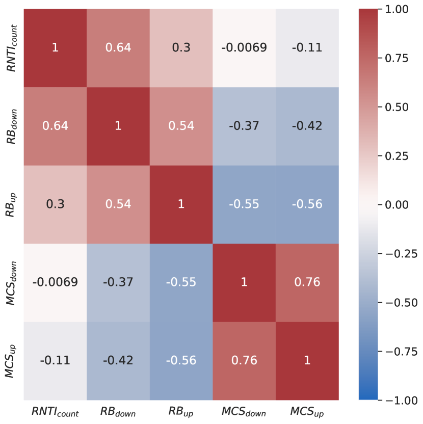
Figure 1: Average Pearson coefficients matrix of the three datasets.

We compute the correlation among the considered variables in Fig. 1 using Pearson coefficient. The matrix shows poor correlation among the 5 data features. In particular, we note that RB_down is more correlated to RNTI_count than RB_up. This is due to the fact that downlink traffic is predominant in LTE with respect to uplink. Finally, it is interesting to notice that the MCS columns are negatively correlated to the percentage of assigned RBs: the reason is that a low average MCS, either in the downlink or in the uplink, means that the channel quality is degrading and, therefore, more RBs have to be assigned to transmit the same amount of data.

In Fig. 2 we present a temporal analysis of our dataset during a week. In particular, we show the variation in time for PS data of RNTI_count, RB_down and RB_up, respectively. A clear daily periodicity characterizes the data. The daily periodicity of the data is also revealed by all the other datasets. Slight differences appear only for EB, in which evidently higher picks show up in the weekend nights, reflecting the popularity of the El Born district as a nightlife center of the city.

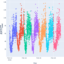
(a)

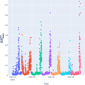
(b)

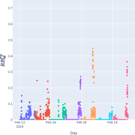
(c)

Figure 2: Variables time series on a sample of 7 days of the PS dataset for RNTI_count (a), RB_down (b) and RB_up (c). Each color corresponds to a day of the week, starting from Monday which is the first represented with blue color.

Finally, we analyze the impact on the scale proportion, and in the dynamics between the downlink and the uplink channels of the three selected datasets. Here, the human behavior in the neighborhoods where the data has been collected is of key importance: Poble-sec is mainly a residential area, instead El Born boasts a lively nightlife and Les Corts hosts the Camp Nou football stadium. For this purpose, we evaluate the total traffic demand as a function of the actual data transmitted. Driven by this aim, we define THR_down and THR_up as a-posteriori estimation of the cumulative Transport Block Size (TBS) in bits in downlink and uplink, respectively, evaluated according to 3GPP specifications [25]. These metrics are reported in Fig. 3 for the different datasets during a week, for the sake of readability. The patterns between the uplink and downlink channels is similar for PS and EB datastes, instead the range of values significantly differs, being THR_up lower than THR_down. Alternatively, for LC, THR_down is much smaller with respect to the other databases, and THR_up shows peaks higher than THR_down. These peaks correspond with periods when football matches occur in the Camp Nou stadium, located near the base station. We refer to our previous papers [26] and [27] for a more comprehensive study on mobile traffic analysis during these events.

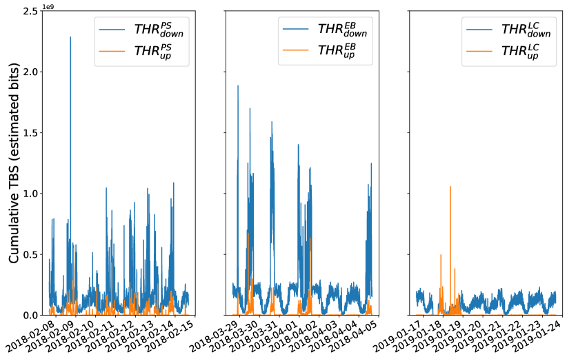
Figure 3: THR_down and THR_up time series by date for the three datasets on a sample of 7 days.

IV Traffic Prediction Models

IV-A Problem Statement

Let $\mathcal{T}$ be the total measurement period of a given dataset. For every time $t\in\mathcal{T}$, let us define $\bm{x}(t)$ as the vector containing the $m$ input features. Note that $\mathcal{T}$ changes for each dataset and this formulation is intended to be general for all of them. Similarly, the time interval $[t,t+1]$ is 2 minutes for every dataset, as justified in Section III. The prediction model is organized as follows. Let $p$ be the number of input observations (samples), in terms of the number of dataset entries, constituting a single input instance, i.e., each input frame of the models will have shape $p\times m$: $\{\bm{x}(t),\bm{x}(t+1),...,\bm{x}(t+p-1)\}$. Let $\Delta n$ be the time of the output frame to be predicted in terms of number of samples with respect to the input frame, i.e., for a specific input frame $\bm{x}(t)$ the prediction will be the vector of $q$ variables $\bm{y}(t+\Delta n)$. We studied the cases with $p\in\{10,15,20\}$ and $\Delta n\in\{0,4,9,14\}$; in other words, we considered, respectively, $20$, $30$ and $40$ minutes of past data to predict samples expected $2$, $10$, $20$ and $30$ minutes after.

Given the multiple variables of $\bm{x}(t)$, we perform data normalization for all the columns in each dataset in the interval $[-1,1]$ to keep the data symmetric to the activation functions of the DL models used (i.e., the tanh). Moreover, we apply data windowing to the sequence $\bm{x}(t)$, which is split and grouped using a fixed-length window of $p$ samples. The window is moved each time by one-step. The value of $p$ defines how many time-lags are processed by the DL models. The multi-variate sequence can be expressed as $\left[\bm{x}(1),\bm{x}(2),\dots,\bm{x}(T)\right]$, where $T$ is the cardinality of $\mathcal{T}$, i.e., $T=|\mathcal{T}|$. After the split, we have $N=T-p+1$ sequences $\mathbf{x}(n)$, $n\in[1,N]$:

$$\mathbf{x}(1)=\left[\bm{x}(1),\bm{x}(2),\dots,\bm{x}(p)\right]$$

$$\mathbf{x}(2)=\left[\bm{x}(2),\dots,\bm{x}(p+1)\right]$$

$$\mathbf{x}(N)=\left[\bm{x}(N),\dots,\bm{x}(T)\right]$$

A sequence $\mathbf{x}(n)$ has length $p$ and each of its element is $m$-dimensional. Hereafter, we refer to the sequence $\mathbf{x}$ as samples. Then, we define $\mathbf{X}$ as the three-dimensional matrix which contains $N$ sequences of $\mathbf{x}$. The matrix $\mathbf{X}$ has dimension $N\times p\times m$ and serve as input tensor to the DL algorithms.

We choose the multivariate input and output of the prediction model based on the EDA in Section III and driven by the physical meaning of the features. The resulting input features are the following $m=5$ variables: RNTI_count, RB_down, RB_up, MCS_down and MCS_up. Regarding the output, we select $q=5$ variables used in our prediction models because of their valuable meaning for network operators, and in particular we choose RNTI_count, RB_down, RB_up, THR_down and THR_up. The reason behind this choice is that these variables represent key performance indicators for network management, including bandwidth allocation, QoS provisioning, energy-saving, interference management, etc.

In what follows, we tailor different DL architectures for our mobile traffic prediction problem. In particular, our models are based on RNN and CNN architectures to exploit the temporal characteristics of the datasets under study. Our proposal accounts for both stand-alone models and the KTL paradigm.

IV-B RNN Model

Among the several RNNs DL models, we adopt Gated Recurrent Units (GRUs) due to their high effectiveness and major simplicity, with respect to other popular architectures, such as the LSTM cells [28].

][b].49

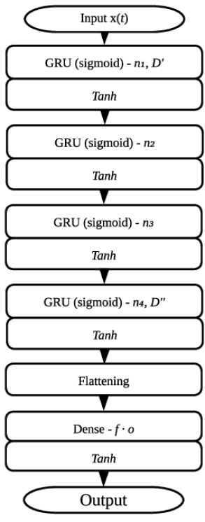
(a) GRU

][b].49

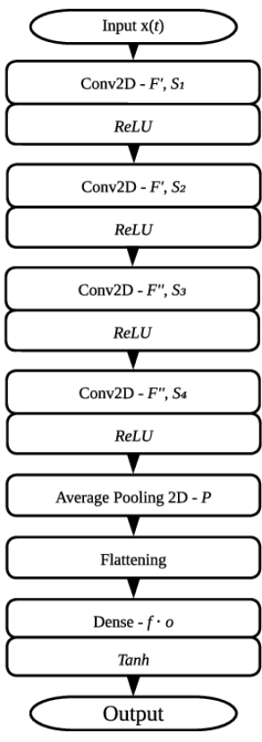
(b) CNN

Figure 4: Models’ structure representation.

After a comprehensive assessment of different configurations for the network structure, the architecture shown in Fig. 4(a) proves to be the best for the considered task. The intuition behind its effectiveness is that we aim to create higher-level abstractions and capture more nonlinearity between the data thanks to the stacked layers. Moreover, we intent to enforce the data correlation with the previous inputs, which is provided by the structure of each GRU cell. In detail, after the input layer, we insert a first recurrent layer, containing $n_{1}$ GRU cells with sigmoid activation for the input, forget and output gates, and hyperbolic tangent activation for the hidden and output states; dropout regularization with probability parameter $D^{\prime}$ is also implemented to prevent overfitting. The second and third layer are based on GRU with the same activation function of the first, and contain respectively $n_{2}$ and $n_{3}$, while the fourth layer contains $n_{4}$ such GRU cells and dropout regularization with probability parameter $D^{\prime\prime}$. At the end, the tensor is flattened by introducing the final dense layer containing $q$ neurons, and a hyperbolic tangent activation function is added in order to obtain the prediction in output. Notice that we select the final activation to meet the rescaling interval of the normalized output data ($[-1,1]$), while the choice of adding dropout regularization to the first and last layers of the network is motivated by [29].

The best performing RNN hyperparameters are reported in Table 1a, as result of a grid-search.

IV-C CNN Model

The second DL architecture is based on CNNs. As for RNNs, we tested different network configurations, finally leading to the choice of the structure represented in Figure 4(b). To understand the strength of this architecture, we can think to each input feature as an image, where each value corresponds to a pixel. As a processed input runs deeper in the network, higher-level abstractions of it are extracted and nonlinearly correlated by means of the activation functions. In this case, the advantages consist in a significantly lower number of parameters to be trained and in a natural mitigation of the vanishing gradient problem affecting the RNN architectures. In detail, the input layer is followed by four two dimensional convolutional layers, each accompanied by a Rectified Linear Unit (ReLU) activation layer, with a non-decreasing number of filters and different ad hoc kernel sizes. We choose Leaky ReLU activation functions to solve the well-known problem of trained weights that permanently prevent a set of neurons to be activated and caused by ReLU functions’ zero slope for $x$-axis negative values.

The first two convolutional layers contain $F^{\prime}$ filters, respectively of dimension $S_{1}$ and $S_{2},$ while the third and fourth convolutional layers contain $F^{\prime\prime}$ filters of dimension is $S_{3}$ and $S_{4}.$ The filters’ stride is equal to one in all the cases (one-step on the horizontal movements, and one-step row change on the vertical movements) since the dimensionality of the problem is quite small and we do not want to lose important information. After that, a two dimensional average pooling layer provides a valuable summary of the extracted information along the temporal axis, thanks to the pooling size $P=[2,1]$. Finally, like in the RNNs, a flattening layer is inserted, followed by a final dense layer containing $q$ neurons with hyperbolic tangent activation to obtain the prediction. Note that, in the CNNs’ case, we rearrange the features order as follows: RB${}_{down},$ RB${}_{up},$ RNTI${}_{count},$ MCS${}_{down},$ MCS${}_{up}.$ The reason is to allow the network to exploit the a-priori uncorrelation of RNTI_count with all the other variables, given the local approach of kernels among the features in CNN models.

The best performing CNN hyperparameters resulting from a grid-search are reported in Table 1b. The resulting best value of $S_{1}=[16,3]$ implies that a correlation of a higher number of variables from the first hidden layer can help the model to perform better. In particular, given the filters’ size and the unitary stride, the RNTI_count variable is the only one to get directly involved with all the other features in the CNN convolutions since the layer closest to the input of the network. $S_{2}=[3,5]$, being the best choice for the second layer filters dimension, indicates that correlating all the five input variables three time steps at a time is the best trade-off to maximize the extracted information. Furthermore, $F^{\prime\prime}=32$, as the ideal number of filters for both the third and the fourth layers, suggests that too many filters are not needed when their size is chosen properly, being $S_{3}=[8,3]$ and $S_{4}=[4,3]$ in our case. Finally, $P=[2,1]$ confirms that the average pooling layer is useful to provide a summary of the convolutional layers’ output along the temporal axis. However, it also reveals that it only needs to involve two rows to retrieve the relevant insights extracted from the internal layers and provide a reliable prediction.

$n_{1}$	$n_{2}$	$n_{3}$	$n_{4}$	$D^{\prime}$	$D^{\prime\prime}$
$128$	$64$	$32$	$16$	$0$	$0.2$

(a)

$F^{\prime}$	$F^{\prime\prime}$	$S_{1}$	$S_{2}$	$S_{3}$	$S_{4}$	$P$
$16$	$32$	$[16,3]$	$[3,5]$	$[8,3]$	$[4,3]$	$[2,1]$

(b)

TABLE 1: DL models’ optimized hyperparameters.

IV-D Knowledge Transfer

The adopted KTL method is a network-based deep transfer learning, which reuses part of the network that have been pre-trained in the source domain. In particular, it consists on freezing the neurons placed in different combinations of layers, i.e., inhibiting the update of neurons’ weight, and thus training the remaining part of the networks on the new data [30]. This approach is based on the assumption that, for both RNNs and CNNs, each layer extracts meaningful features from the output of the previous one. This implies that groups of neurons which are close (considering the adopted metric on the network graph) should be specified in extracting similar types of information.

The idea is to perform a new training only on the part of the network which is responsible of extracting the features devoted to describe the differences among the datasets. Thus, the common general information already obtained by the source model (and maintained by the frozen neurons) are preserved, while the model is adapting the prediction to the new input distribution.

V Experiments and results

The following section details the characteristics of the experiments performed and the numerical results of the different models. For the sake of clarity, the section is divided into five subsections. In Section V-A the model training setup is detailed. Section V-B reports the performance of the stand-alone models on the PS, EB and LC datasets, respectively. The usage of KTL and its performance is detailed in Section V-C. Model complexity and the energy consumption of the studied models are discussed in Section V-D. Finally, Section V-E contains the comparison with the benchmark SVR models.

V-A Model Training Setup

We split each dataset into a training $\mathcal{D}_{t,i}$ and a validation set $\mathcal{D}_{v,i}$, being each of them, in turn, divided in two additional different proportions ($i\in[1,2]$) to study the best threshold between the size of the training set $|\mathcal{D}_{t}|$ and the performance of each model. In particular, $\mathcal{D}_{t,1}^{\text{PS}}$ and $\mathcal{D}_{t,2}^{\text{PS}}$ contain respectively fourteen and twenty-one days of data in PS. $\mathcal{D}_{t,1}^{\text{EB}}$ and $\mathcal{D}_{t,1}^{\text{LC}}$ contain, instead, five days of data, whereas $\mathcal{D}_{t,2}^{\text{EB}}$ and $\mathcal{D}_{t,2}^{\text{LC}}$ cover a six days time period. No significant difference was found among the two setups, besides a more consistent convergence of the loss function when training the models on the biggest training set. The results will hence be reported for $\mathcal{D}_{t,2}$ and $\mathcal{D}_{v,2}$ only, referred to as $\mathcal{D}_{t}$ and $\mathcal{D}_{v}$ in the rest of this work.

We have trained and validated the models using an Ubuntu 18.04 High Performance Cluster, with 2 Intel(R) Xeon(R) Gold 6230 CPU @ 2.10GHz, 187 GB of RAM and four NVIDIA GeForce RTX 2080 Ti GPUs. We have implemented the DL algorithms in Python, using the Keras library on top of the Tensorflow backend. For the benchmark SVR, we used the popular Scikit-Learn library.

We assess the regression performance looking at the Mean Squared Error (MSE) between the true validation data and the predictions, divided by the cardinality of the validation set $|\mathcal{D}_{v}|.$ This allows to fairly compare models, which have been trained on different portions of the same dataset. To achieve reliable results, we have run the experiments on each model three times and we have averaged the resulting output metrics.

As number of training epochs, we adopt an upper-bound for all the cases independently from the trained structure and the dataset. This choice aims to reduce the manual intervention in the training process, avoiding to set a customized hyperparameter for each case. We set the number of epochs to 30, also in the KTL framework, where the needed epochs are even fewer. Average values for the actual necessary number of training epochs will be reported in Section V-D.

V-B Stand-alone models

As a first step of our analysis, we train RNN and CNN based models on the data collected from the three locations in Barcelona (PS, EB and LC). The results in terms of MSE for the datasets $\mathcal{D}_{t}^{\text{PS}}$, $\mathcal{D}_{t}^{\text{EB}}$, and $\mathcal{D}_{t}^{\text{LC}}$ are reported in Table 2, Table 3 and Table 4, respectively. In detail, we report the results by varying the input window of observation $p$ in the columns and the time interval from the input and the output tensor $\Delta n$ in the rows. The lowest MSE between the CNN and RNN models performing the same task has been highlighted in yellow to improve the readability of the tables.

$\begin{array}[]{c|cc|cc|cc|c}\Delta n\backslash p&\lx@intercol\hfil 10\hfil\lx@intercol\vrule\lx@intercol&\lx@intercol\hfil 15\hfil\lx@intercol\vrule\lx@intercol&\lx@intercol\hfil 20\hfil\lx@intercol\vrule\lx@intercol&\\ \hline\cr 0&0.0091&\pagecolor[HTML]{FFF4BD}0.0088&\pagecolor[HTML]{FFF4BD}0.0087&0.0089&\pagecolor[HTML]{FFF4BD}0.0088&0.0090&\text{MSE}\\ \hline\cr 4&\pagecolor[HTML]{FFF4BD}0.0153&0.0156&0.0149&\pagecolor[HTML]{FFF4BD}0.0148&\pagecolor[HTML]{FFF4BD}0.0151&0.0155&\text{MSE}\\ \hline\cr 9&\pagecolor[HTML]{FFF4BD}0.0175&0.0176&0.0183&\pagecolor[HTML]{FFF4BD}0.0174&0.0184&\pagecolor[HTML]{FFF4BD}0.0180&\text{MSE}\\ \hline\cr 14&0.0197&\pagecolor[HTML]{FFF4BD}0.0196&\pagecolor[HTML]{FFF4BD}0.0193&\pagecolor[HTML]{FFF4BD}0.0193&0.0198&\pagecolor[HTML]{FFF4BD}0.0192&\text{MSE}\\ \hline\cr&\text{RNN}&\text{CNN}&\text{RNN}&\text{CNN}&\text{RNN}&\text{CNN}&\\ \end{array}$

TABLE 2: MSE of the stand-alone models trained on $\mathcal{D}_{t}^{\text{PS}}$.

$\begin{array}[]{c|cc|cc|cc|c}\Delta n\backslash p&\lx@intercol\hfil 10\hfil\lx@intercol\vrule\lx@intercol&\lx@intercol\hfil 15\hfil\lx@intercol\vrule\lx@intercol&\lx@intercol\hfil 20\hfil\lx@intercol\vrule\lx@intercol&\\ \hline\cr 0&\pagecolor[HTML]{FFF4BD}0.0062&0.0065&\pagecolor[HTML]{FFF4BD}0.0062&0.0070&\pagecolor[HTML]{FFF4BD}0.0063&0.0068&\text{MSE}\\ \hline\cr 4&0.0083&\pagecolor[HTML]{FFF4BD}0.0079&\pagecolor[HTML]{FFF4BD}0.0081&\pagecolor[HTML]{FFF4BD}0.0081&0.0084&\pagecolor[HTML]{FFF4BD}0.0076&\text{MSE}\\ \hline\cr 9&0.0081&\pagecolor[HTML]{FFF4BD}0.0079&\pagecolor[HTML]{FFF4BD}0.0081&0.0088&\pagecolor[HTML]{FFF4BD}0.0078&0.0087&\text{MSE}\\ \hline\cr 14&0.0090&\pagecolor[HTML]{FFF4BD}0.0089&0.0099&\pagecolor[HTML]{FFF4BD}0.0092&\pagecolor[HTML]{FFF4BD}0.0089&0.0090&\text{MSE}\\ \hline\cr&\text{RNN}&\text{CNN}&\text{RNN}&\text{CNN}&\text{RNN}&\text{CNN}&\\ \end{array}$

TABLE 3: MSE of the stand-alone models trained on $\mathcal{D}_{t}^{\text{EB}}.$

$\begin{array}[]{c|cc|cc|cc|c}\Delta n\backslash p&\lx@intercol\hfil 10\hfil\lx@intercol\vrule\lx@intercol&\lx@intercol\hfil 15\hfil\lx@intercol\vrule\lx@intercol&\lx@intercol\hfil 20\hfil\lx@intercol\vrule\lx@intercol&\\ \hline\cr 0&\pagecolor[HTML]{FFF4BD}0.0089&\pagecolor[HTML]{FFF4BD}0.0089&\pagecolor[HTML]{FFF4BD}0.0086&0.0090&\pagecolor[HTML]{FFF4BD}0.0089&\pagecolor[HTML]{FFF4BD}0.0089&\text{MSE}\\ \hline\cr 4&0.0144&\pagecolor[HTML]{FFF4BD}0.0141&\pagecolor[HTML]{FFF4BD}0.0136&0.0141&\pagecolor[HTML]{FFF4BD}0.0137&0.0141&\text{MSE}\\ \hline\cr 9&\pagecolor[HTML]{FFF4BD}0.0164&\pagecolor[HTML]{FFF4BD}0.0164&0.0166&\pagecolor[HTML]{FFF4BD}0.0159&\pagecolor[HTML]{FFF4BD}0.0161&0.0165&\text{MSE}\\ \hline\cr 14&0.0187&\pagecolor[HTML]{FFF4BD}0.0184&0.0187&\pagecolor[HTML]{FFF4BD}0.0183&\pagecolor[HTML]{FFF4BD}0.0190&\pagecolor[HTML]{FFF4BD}0.0190&\text{MSE}\\ \hline\cr&\text{RNN}&\text{CNN}&\text{RNN}&\text{CNN}&\text{RNN}&\text{CNN}&\\ \end{array}$

TABLE 4: MSE of the stand-alone models trained on $\mathcal{D}_{t}^{\text{LC}}.$

In most cases, the MSE increases with $\Delta n$, as expected. For example, the MSE for $\Delta n=14$ doubles that of $\Delta n=0$ with datasets $\mathcal{D}_{t}^{\text{PS}}$ and $\mathcal{D}_{t}^{\text{LC}}$. Interestingly, RNNs seem to perform better with small values of $\Delta n,$ whereas CNNs outperform for higher values. This phenomenon can be motivated by CNNs being able to better represent the temporal structure of input signals for longer time horizons, which leads to better predictions for higher $\Delta n$.

Another noticeable trend is that MSE values are stable with $p$ for both RNNs and CNNs. This result suggests that the information temporally far from the models’ output does not contribute in improving its prediction accuracy. This property will be confirmed by the XAI tools in Section VI.

V-C KTL models

For this analysis, we consider the larger PS dataset as the teacher, who transfers the knowledge obtained in the stand-alone model to the other two (student) datasets (EB and LC). We follow the approach in [30], which consists of building the new (student) model by selecting a subset of layers of the teacher model (those closer to the input) as trained on the teacher dataset (operation called layer freezing). Instead, the remaining layers, and closer to the output, are re-trained based on the new (student) data. The rationale is based on the assumption that each layer is able to extract meaningful and gradually more specific features. Therefore, layers closer to the output are supposed to be those extracting features for that specific learning task, in our case the traffic prediction of the student in the new location. Consequently, in this work, we study the model behavior when re-training part of the layers close to the output. In particular, we consider all the possible combinations in re-training each of the last three layers of the two DL models. One of these combinations includes also the teacher model trained with PS dataset (i.e., student model with all frozen layers from the teacher). This instance is the extreme example of knowledge transfer without any extra training cost.

In Table 5 we show the lowest MSE of the models among the different freezing combinations using KTL on EB data, using $\mathcal{D}_{t}^{\text{PS}}$ to train the teacher model. Similarly, Table 6 provides the same results for the LC dataset. The blue color highlights which of the two considered DL models returns the lowest MSE.

$\begin{array}[]{c|cc|cc|cc|c}\Delta n\backslash p&\lx@intercol\hfil 10\hfil\lx@intercol\vrule\lx@intercol&\lx@intercol\hfil 15\hfil\lx@intercol\vrule\lx@intercol&\lx@intercol\hfil 20\hfil\lx@intercol\vrule\lx@intercol&\\ \hline\cr$0$&\pagecolor[HTML]{CEE5ED}0.0060&\pagecolor[HTML]{CEE5ED}0.0060&\pagecolor[HTML]{CEE5ED}0.0059&0.0060&0.0060&\pagecolor[HTML]{CEE5ED}0.0059&\text{MSE}\\ \hline\cr$4$&\pagecolor[HTML]{CEE5ED}0.0077&0.0079&0.0078&\pagecolor[HTML]{CEE5ED}0.0074&\pagecolor[HTML]{CEE5ED}0.0077&0.0078&\text{MSE}\\ \hline\cr$9$&0.0081&\pagecolor[HTML]{CEE5ED}0.0078&0.0085&\pagecolor[HTML]{CEE5ED}0.0079&\pagecolor[HTML]{CEE5ED}0.0080&0.0082&\text{MSE}\\ \hline\cr$14$&0.0092&\pagecolor[HTML]{CEE5ED}0.0089&0.0096&\pagecolor[HTML]{CEE5ED}0.0088&0.0096&\pagecolor[HTML]{CEE5ED}0.0091&\text{MSE}\\ \hline\cr&\text{RNN (T)}&\text{CNN (T)}&\text{RNN (T)}&\text{CNN (T)}&\text{RNN (T)}&\text{CNN (T)}&\\ \end{array}$

TABLE 5: MSE of the best transferred models for each of the considered cases, trained on $\mathcal{D}_{t}^{\text{EB}}.$

$\begin{array}[]{c|cc|cc|cc|c}\Delta n\backslash p&\lx@intercol\hfil 10\hfil\lx@intercol\vrule\lx@intercol&\lx@intercol\hfil 15\hfil\lx@intercol\vrule\lx@intercol&\lx@intercol\hfil 20\hfil\lx@intercol\vrule\lx@intercol&\\ \hline\cr$0$&\pagecolor[HTML]{CEE5ED}0.0084&\pagecolor[HTML]{CEE5ED}0.0084&\pagecolor[HTML]{CEE5ED}0.0085&\pagecolor[HTML]{CEE5ED}0.0085&\pagecolor[HTML]{CEE5ED}0.0085&\pagecolor[HTML]{CEE5ED}0.0085&\text{MSE}\\ \hline\cr$4$&\pagecolor[HTML]{CEE5ED}0.0136&\pagecolor[HTML]{CEE5ED}0.0136&0.0135&\pagecolor[HTML]{CEE5ED}0.0134&\pagecolor[HTML]{CEE5ED}0.0135&\pagecolor[HTML]{CEE5ED}0.0135&\text{MSE}\\ \hline\cr$9$&\pagecolor[HTML]{CEE5ED}0.0162&0.0164&0.0163&\pagecolor[HTML]{CEE5ED}0.0160&0.0161&\pagecolor[HTML]{CEE5ED}0.0160&\text{MSE}\\ \hline\cr$14$&0.0183&\pagecolor[HTML]{CEE5ED}0.0180&0.0184&\pagecolor[HTML]{CEE5ED}0.0181&0.0181&\pagecolor[HTML]{CEE5ED}0.0180&\text{MSE}\\ \hline\cr&\text{RNN (T)}&\text{CNN (T)}&\text{RNN (T)}&\text{CNN (T)}&\text{RNN (T)}&\text{CNN (T)}&\\ \end{array}$

TABLE 6: MSE of the best transferred models for each of the considered cases, trained on $\mathcal{D}_{t}^{\text{LC}}.$

The trends observed for the stand-alone models with respect to $\Delta n$ and $p$ are maintained. However, the CNN models have usually better accuracy than RNNs. In fact, GRU models extract task-specific features already from the first layers. Therefore, re-trained layers are not able to adapt to the change of domain as accurately as CNNs. This behavior could depend on CNN-based models holding a more hierarchical knowledge distillation architecture, in which the deepest layers are specialized for the specific prediction task to be performed.

Interestingly, no significant difference can be identified whether applying KTL from a teacher model using $\mathcal{D}_{t,1}^{\text{PS}}$ or $\mathcal{D}_{t,2}^{\text{PS}}$. This result suggests that fourteen days of data are enough to train the ML model for extracting the traffic patterns and being able to transfer them to a student model.

Finally, KTL enables an accuracy improvement in more than $85\%$ of the studied cases ($41$ out of $48$) with respect to the stand-alone counterpart. This result confirms that knowledge transfer is a valid method to accurately train models when available data are scarce (as in the case of EB and LC).

V-D Complexity analysis and Energy Cost

Following the Green AI principles [3], we compute the number of training parameters, the training epochs and the training time to have a comprehensive analysis on the complexity of building one model. In particular, we provide the average training time of a single model among the different values of $\Delta n$, to have a more reliable estimation of the required resources, given that the temporal distance of the prediction from the input instances does not affect the training time. Moreover, the drained total training energy is calculated using the online tool Green Algorithms [31]. Results are reported in Table 7 for both stand-alone and KTL cases and using $\mathcal{D}_{t}^{\text{EB}}.$

RNN models contain a total of $100\,981$ parameters. Instead CNN-based models have a number of parameters varying with $p$ and namely $33\,285$, $34\,885$ or $37\,285$, with $p$ equal to $10,$ $15$ or $20$, respectively. In fact, for CNNs with fixed filter sizes in each layer, the number of input values to the final dense layer depends on the number of the filters’ strides. This reflects in a linear increase of the number of weights for each output neuron. Complexity metrics vary very little for CNNs as function of $p$, hence in the table we have reported only values for $p=10$. The number of parameters for CNN based stand-alone models is roughly one third of the corresponding RNNs. This highlights the intrinsic advantage of the convolutional layers, which is reflected in the reduced number of training epochs to reach the minimum loss and the training time that is 10 times lower than RNN. In turn, this difference impacts on the energy footprint, which is 10 times lower for CNNs.

TABLE 7: Model training complexity and energy consumption for both stand-alone and KTL models, trained on $\mathcal{D}_{t}^{\text{EB}}$, $p=10$.

	Stand-alone		KTL
	RNN	CNN	RNN	CNN
N. of parameters	100 981	33 285	9 449.25	13 321.25
N. of training epochs	13	9	6	8
Training time [s]	74.409	3.908	3.804	1.586
Energy drained [Wh]	19.8	1.0	1.0	0.4
% of saved energy by KTL	-	-	94.95	60.00

Considering the KTL models, RNNs need a smaller number of epochs to reach the loss minimum. However, CNN models require less than half of the RNNs training time. This translates into a lower energy footprint of CNNs, which is 40% with respect to RNNs, as for stand-alone models. We can argue that the energy footprint figures are tightly related to the training time, as experienced both for KTL and stand-alone; thus, CNNs represent the most energy efficient model. On the other hand, the gain of KTL in RNN with respect to stand-alone models is of 95%, whereas the CNN architectures reach the 60%, as detailed in Table 7. Consequently, KTL has been able to reduce more the energy usage in the case of the stand-alone model that presents the highest complexity (RNN).

Concluding, we stress that, in addition to substantially decreasing the used energy, KTL also enables an accuracy improvement in $41$ out of $48$ (85%) studied cases with respect to the stand-alone counterpart.

V-E Comparison with Benchmark

In this subsection, we compare the proposed RNN and CNN-based models with a benchmark based on SVR [32]. We apply a transformation based on the Radial Basis Function (RBF) kernel [33] to handle the nonlinearity of our datasets. We consider the best performing hyperparameters, which are the result of a grid-search carried out considering several values of the margin width $\epsilon$ and the regularization parameter $C$.

$\begin{array}[]{c|c|c|c|c|c|c|c|c|c|c}&\lx@intercol\hfil\text{Poble Sec}\hfil\lx@intercol\vrule\lx@intercol&\lx@intercol\hfil\text{El Born}\hfil\lx@intercol\vrule\lx@intercol&\lx@intercol\hfil\text{Les Corts}\hfil\lx@intercol\vrule\lx@intercol&\\ \hline\cr\Delta n\backslash p&10&15&20&10&15&20&10&15&20&\\ \hline\cr 0&\pagecolor[HTML]{EFBE7D}0.0086&0.0087&\pagecolor[HTML]{EFBE7D}0.0087&\pagecolor[HTML]{EFBE7D}0.0061&0.0062&0.0063&\pagecolor[HTML]{EFBE7D}0.0085&0.0086&\pagecolor[HTML]{EFBE7D}0.0086&\text{MSE}\\ \hline\cr 4&0.0153&\pagecolor[HTML]{C1E1C1}0.0152&\pagecolor[HTML]{C1E1C1}0.0153&\pagecolor[HTML]{FAA0A0}0.0075&\pagecolor[HTML]{EFBE7D}0.0077&0.0076&\pagecolor[HTML]{EFBE7D}0.0138&\pagecolor[HTML]{C1E1C1}0.0137&0.0137&\text{MSE}\\ \hline\cr 9&\pagecolor[HTML]{C1E1C1}0.0181&\pagecolor[HTML]{C1E1C1}0.0181&\pagecolor[HTML]{C1E1C1}0.0181&\pagecolor[HTML]{C1E1C1}0.0080&\pagecolor[HTML]{EFBE7D}0.0080&\pagecolor[HTML]{C1E1C1}0.0081&0.0164&\pagecolor[HTML]{C1E1C1}0.0163&\pagecolor[HTML]{C1E1C1}0.0164&\text{MSE}\\ \hline\cr 14&\pagecolor[HTML]{C1E1C1}0.0202&\pagecolor[HTML]{C1E1C1}0.0202&\pagecolor[HTML]{C1E1C1}0.0204&\pagecolor[HTML]{CFCFC4}0.0087&\pagecolor[HTML]{CFCFC4}0.0088&\pagecolor[HTML]{C1E1C1}0.0091&0.0184&\pagecolor[HTML]{C1E1C1}0.0186&\pagecolor[HTML]{EFBE7D}0.0189&\text{MSE}\\ \end{array}$

TABLE 8: MSE of the benchmark SVR models for each of the considered cases, trained on $\mathcal{D}_{t}^{\text{PS}},$ $\mathcal{D}_{t},^{\text{EB}}$ and $\mathcal{D}_{t}^{\text{LC}}.$

Table 8 contains the results of the SVR model in terms of MSE as function of $\Delta n$ and $p$. For PS, which is used for stand-alone models only, we have highlighted in orange the entries where the SVR model performs better, in green when performing worse and left blank (no colour) when the performance are the same. For the EB and LC, used for both stand-alone and KTL models, we adopted a different colour mapping. A red filled cell indicates better MSE of SVR compared to both the stand-alone and KTL models; a gray filled cell a MSE equal to the KTL model, but better than the stand-alone; blank cell a MSE equal to the stand-alone model, but worse than the KTL; a green filled cell indicates a MSE worse than both the stand-alone and KTL models.

SVR performs better for low values of $p$ and $\Delta n$. This is due to the fact that in such cases the task is easier, since the amount of input data is the smallest among all the studied cases and the prediction is closer in time to the input frame. This can be spotted looking at the high concentration of green filled cells for $\Delta n$ equal to $9$ and $14$. Similarly, SVR performance is often comparable or better than DL models in EB and LC due to the smaller cardinality of these training sets. This is highlighted in the table by the high number of orange and red filled cells in the columns of EB and LC.

Therefore, in many cases SVR reaches higher accuracy than the DL models. However, DL models outperform SVR when i) the cardinality of the training set is larger, ii) the dimensionality of the input data increases ($p$) and, iii) the prediction is distant from the input ($\Delta n$). This represents a limit in the generalization properties of SVR applied to big data problems for mobile traffic prediction tasks, as the opposite of the proposed DL models, which scale better in such scenarios.

Moreover, SVR presents important limitation in the applicability of KTL techniques such as layer freezing. In the literature, approaches like Transfer Component Analysis (TCA) [34] can be applied, though they are relying on the processing of the teacher and students datasets combined. Thus, using SVR does not allow to separate the training phase in two (teacher and student learning).

VI Models explainability

We tailor two fairly known XAI algorithms, namely SmoothGrad [10] and LRP [11], to provide interpretable insights into the introduced RNN and CNN-based models.

Model interpretation through SmoothGrad rests upon the definition of the sensitivity maps $M_{i}(\bm{x}(n))$, which aims to differentiate the prediction function $S_{i}(\bm{x}(n))$ for each output feature $i\in[1,\dots,q]$ with respect to the input $\bm{x}(n)$. We follow the algorithm proposed in [10], in which the authors modified its standard calculation to compensate the rapid fluctuations of the computed partial derivatives. The final sensitivity map is resulting from the average of $N$ sensitivity maps $M_{i}(\bm{x}(n))$ computed on different perturbed versions of $\bm{x}(n)$ through Gaussian kernels, and in detail:

$$\hat{M}_{i}(\bm{x}(n))=\frac{1}{N}\sum_{k=1}^{N}M_{i}\left(\bm{x}(n)+\epsilon_{k}\right)\text{ with }i\in[1,\dots,q].$$ (1)

where ($\epsilon_{1},\dots,\epsilon_{N}$) are sampled from a Gaussian random variable $\mathcal{N}\left(0,\sigma^{2}\right)$, and $\sigma$ measures the intensity of the perturbation.

Instead, LRP defines the metric relevance, which is calculated in an iterative fashion from the output to the input neurons. The idea is to start with a neuron $k$ representing the output layer and calculates the relevance value of the neuron at the previous layer $j$ using this equation:

$$R_{j}=\sum_{k}\frac{a_{j}w_{jk}}{\sum_{0,j}a_{j}w_{jk}}R_{k}$$ (2)

where $a_{j}$ denotes the activation of the neuron $j$, and $w_{jk}$ is the weight between the two neurons $i$ and $j$. This formula is used iteratively to calculate the relevance $R$ for every neuron of the previous layer. The process is then repeated layer by layer until reaching the input. The obtained final metric (from output to input layers) shows which input features are most relevant to the output.

The two XAI algorithms have been implemented using the iNNvestigate Python library [35].

VI-A Explainability Analysis

It is to be noted that both SmoothGrad and LRP are meant to be applied to a single specific input sample. Instead, here we are more interested to interpret the behavior of our models on the whole dataset; therefore, we have used $\mathcal{D}_{t}^{\text{PS}}$ to obtain the correspondent sensitivity and relevance values. For the sake of visibility, in the next figures we show the squared average of the resulting values and highlight the input features that play a key role in the prediction across the studied dataset, independently to the sign of their contribution. In line with the XAI paradigm, all the processed results have been plotted in groups of five heatmaps, each one corresponding to one of the $q$ output labels, i.e., $RNTI_{count}$, $RB_{down}$, $RB_{up}$, $THR_{down}$, $THR_{up}$. The $x$ axis contains the $m$ input variables, and the $y$ axis shows the progressive temporal index of the $p$ input observations. Sensitivity and relevance are reported in the table with a colour format. Darker shades represent features with higher values, i.e. more important in making predictions.

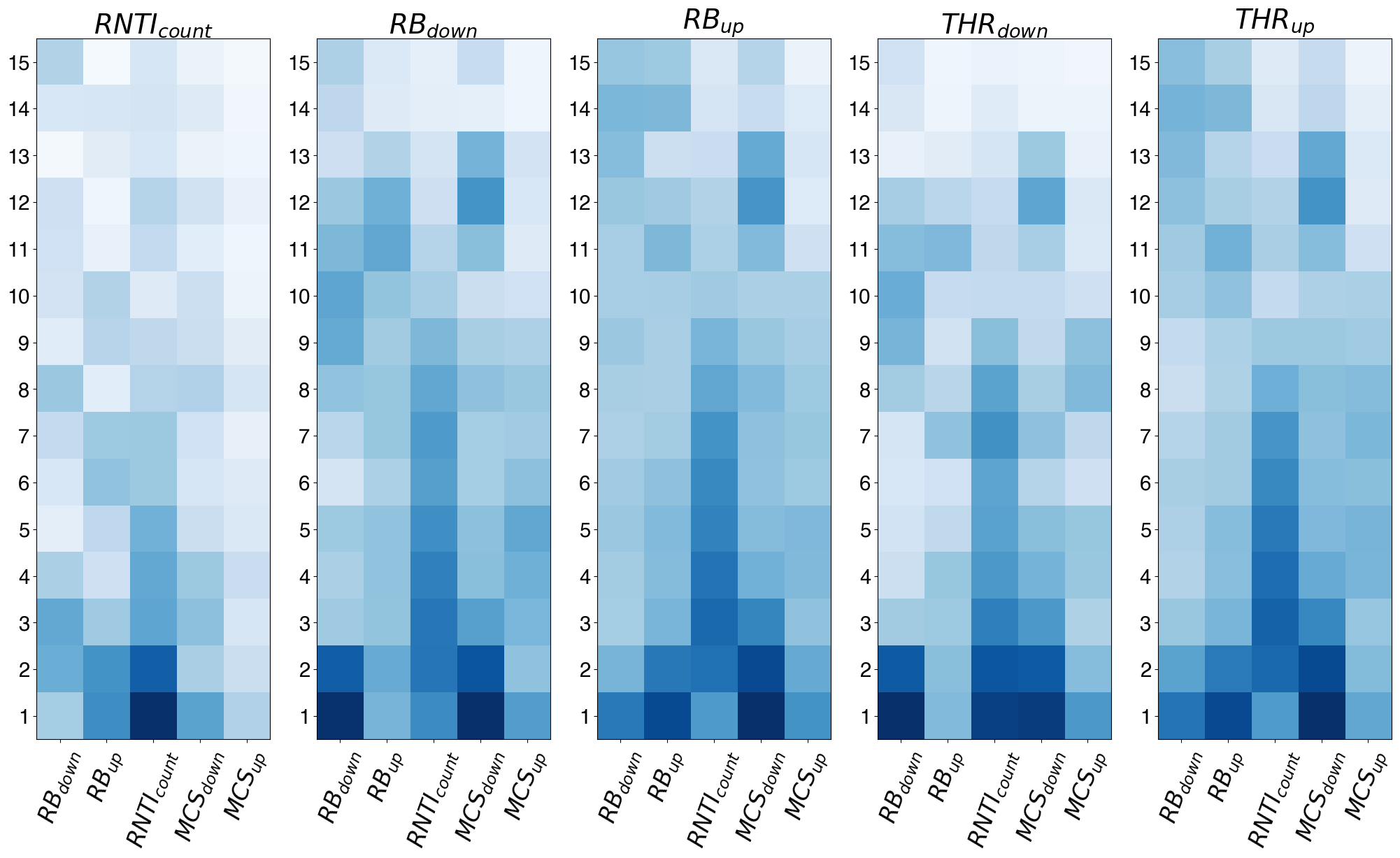
(a) SmoothGrad

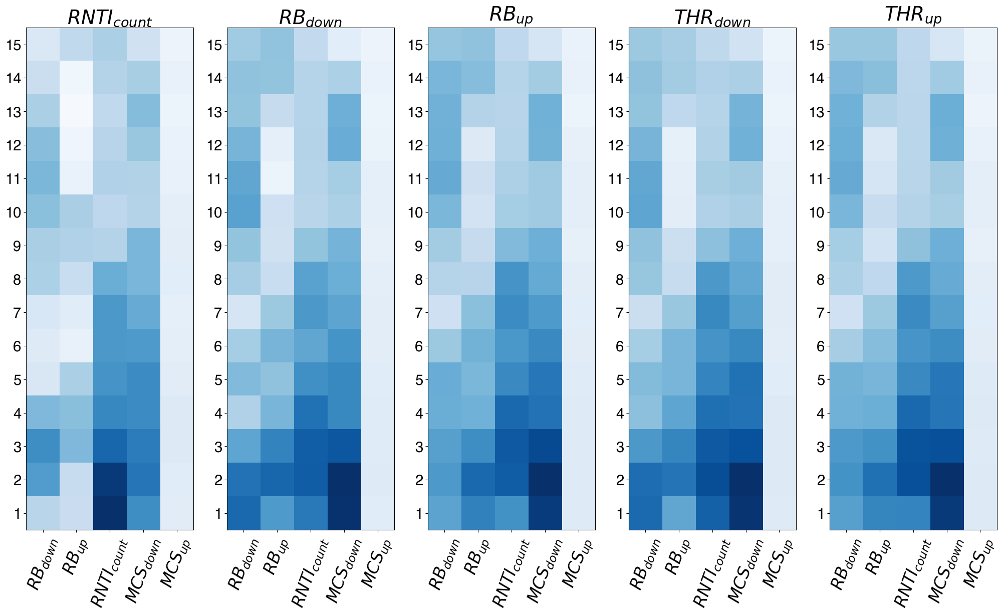
(b) LRP

Figure 6: SmoothGrad and LRP algorithms’ heatmaps when applied to the CNN model, $p=15,$ $\Delta n=0.$

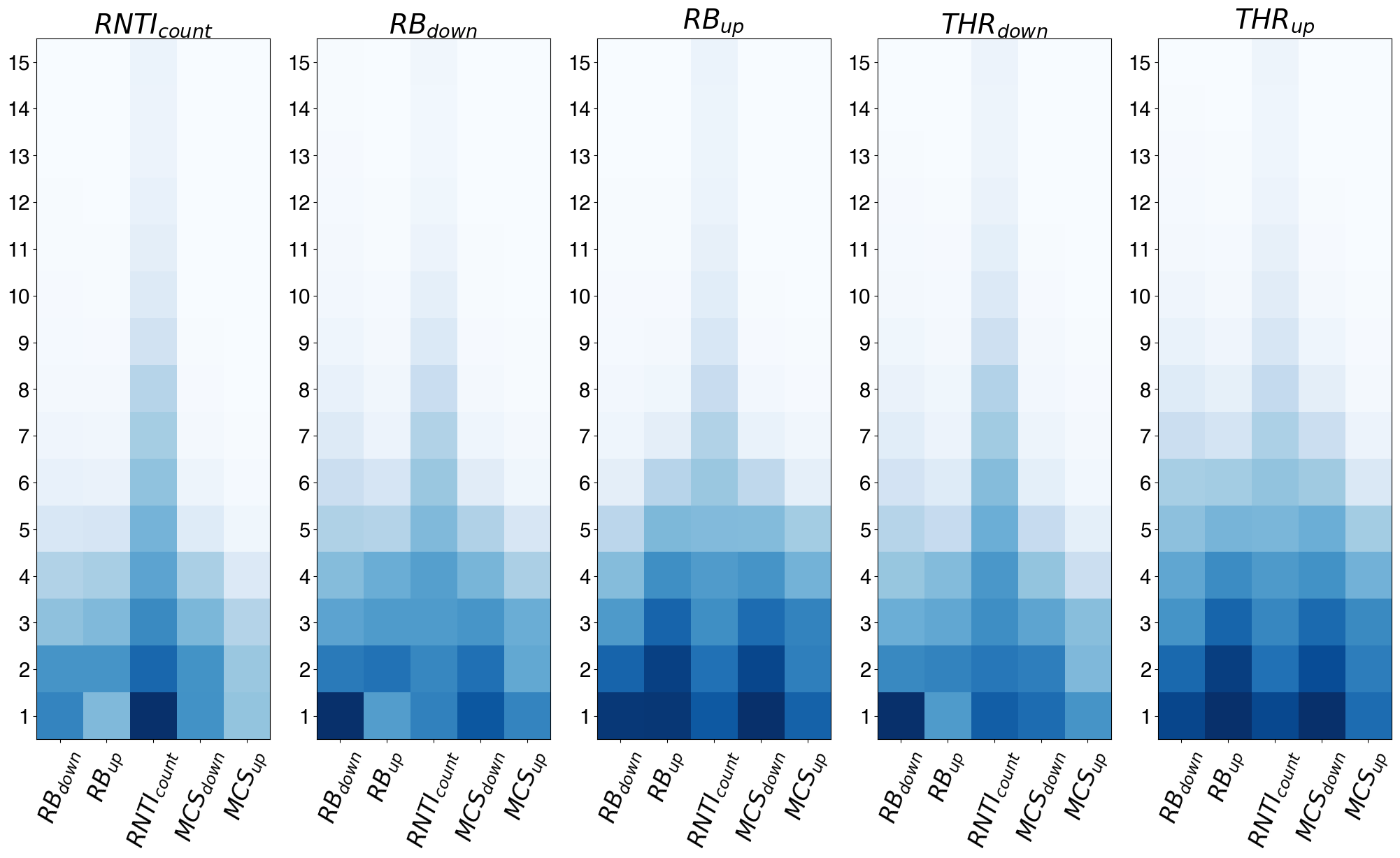
(a) SmoothGrad

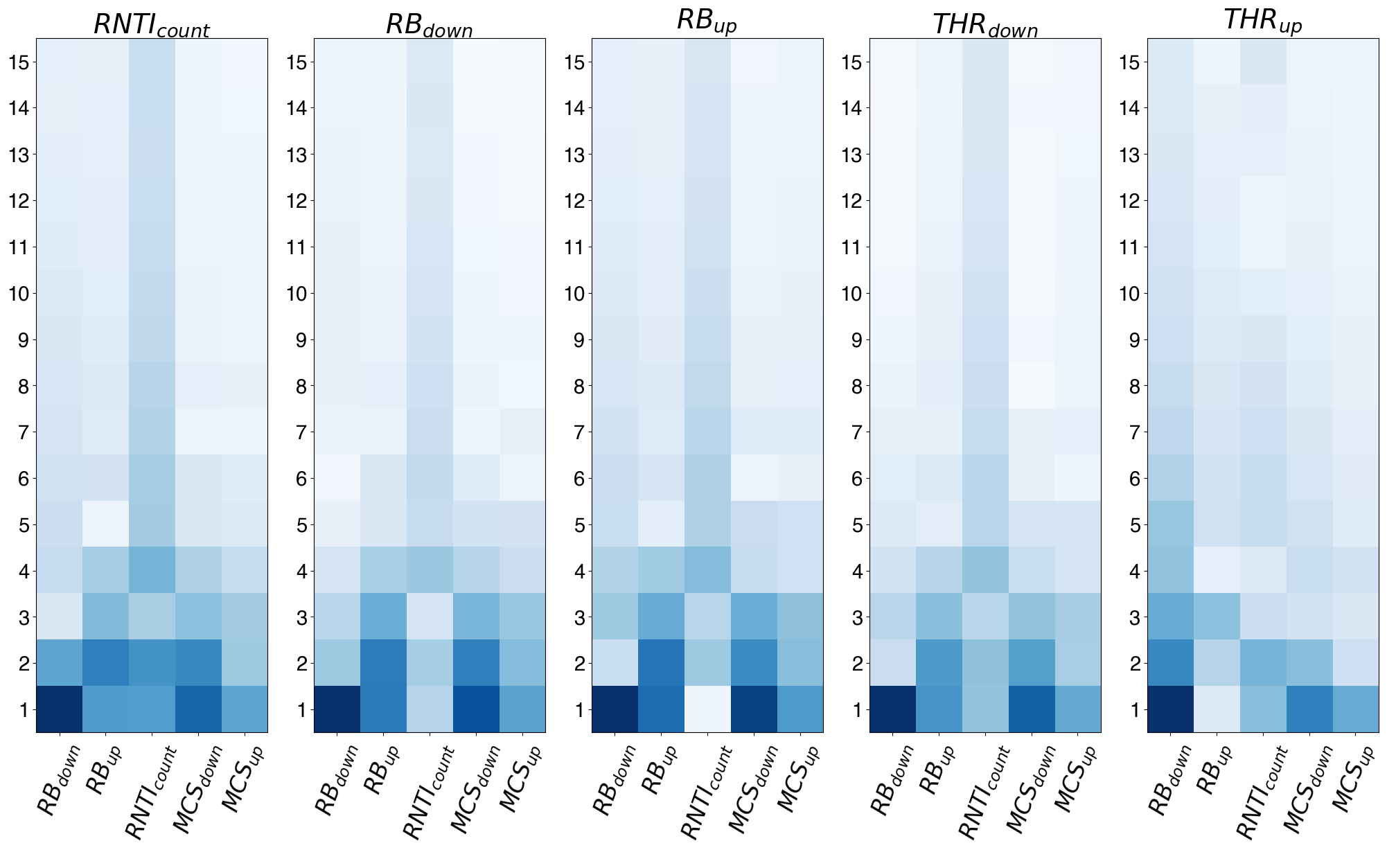
(b) LRP

Figure 7: SmoothGrad and LRP algorithms’ heatmaps when applied to the RNN model, $p=15,$ $\Delta n=0.$

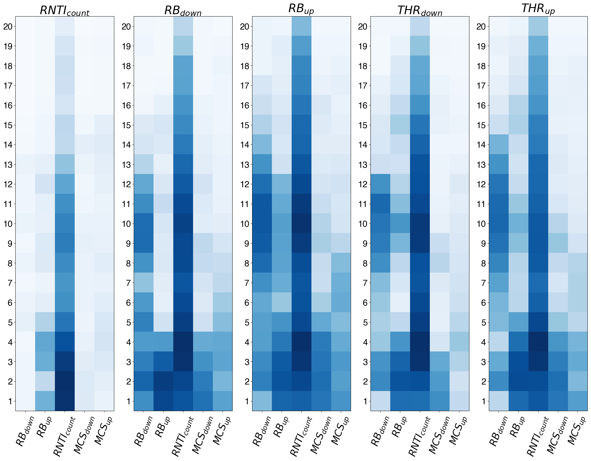
(a) SmoothGrad

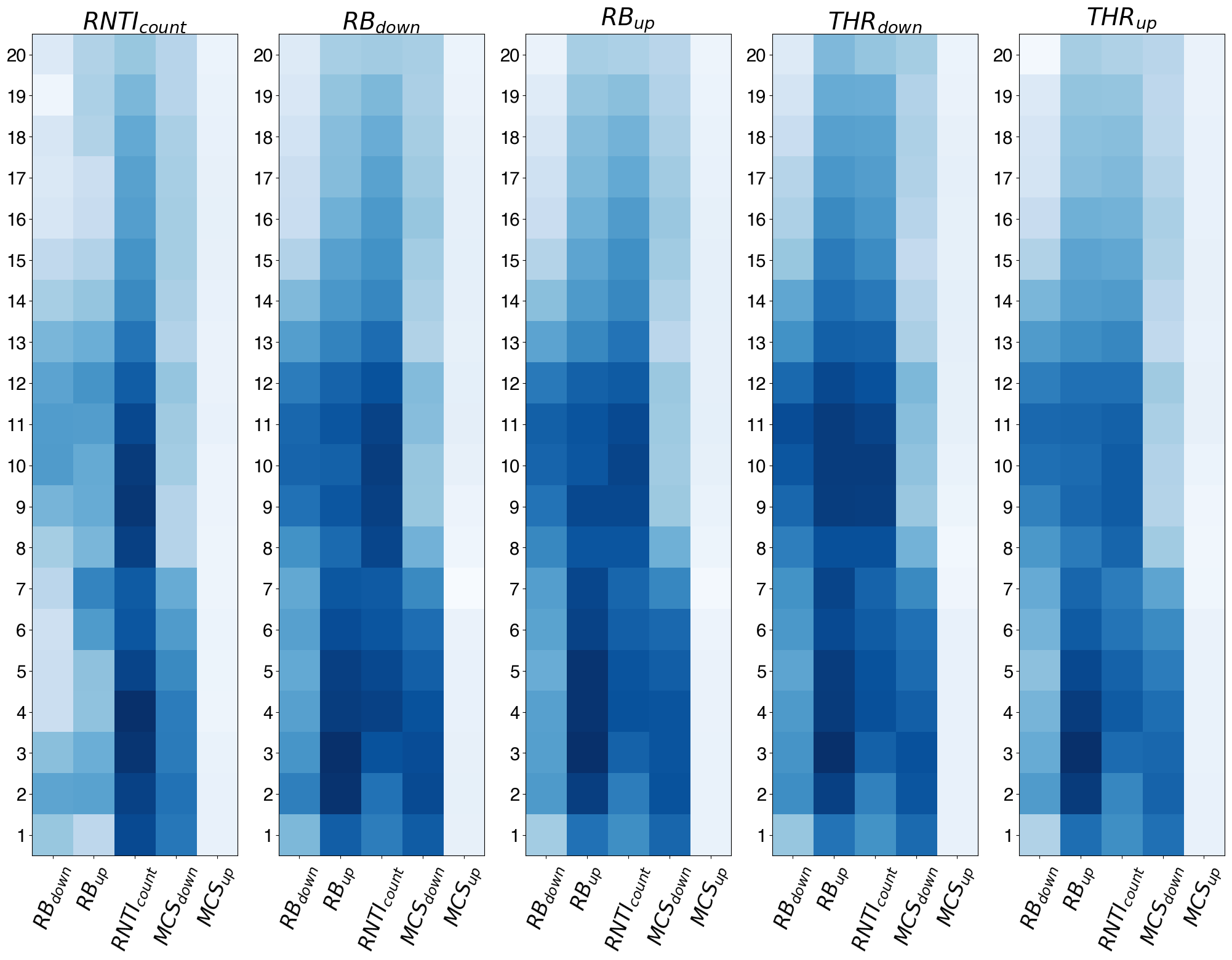
(b) LRP

Figure 8: SmoothGrad and LRP algorithms’ heatmaps when applied to the CNN model, $p=20,$ $\Delta n=14.$

Fig. 6(a) and Fig. 6(b) contain the visual representation of the output heatmaps of the SmoothGrad and LRP algorithms, respectively, applied to the CNN model trained on $\mathcal{D}_{t}^{\text{PS}}$ with a BS of $256$ and with $\Delta n=0$. Fig. 6(a) indicates that the RNTI_count feature is the most informative for predicting RNTI_count. Instead, RB_down and THR_down predictions depend strongly on RB_down and MCS_down; RB_up and THR_up predictions are mainly influenced by MCS_down, RB_up and RNTI_count. This means that forecasting RNTI_count mainly depends on the historical data of the same variable, which is due to the fact that the number of users is the variable with the lowest variance in time as well as to the small $\Delta n$ value. In particular, the low variability allows to make accurate predictions using the last input observations.

LRP heatmap in Figure 6(b) presents similar results with respect to SmoothGrad and confirms the dependencies among input features and predicted labels. Again, it confirms that RNTI_count predictions strongly rely on the historical data of the same variable, as noticed with SmoothGrad. Moreover, MCS_up appears to be almost irrelevant for the predictions (even less than with SmoothGrad), probably due to the limited traffic in uplink from the captured datasets. The entries in the upper part of the heatmaps (i.e, higher $p$) result to be less significant. These results in Fig. 6(a) and Fig. 6(b) confirm our analysis in Section V-B, where we discussed that longer observation windows are not increasing the prediction accuracy. On the other hand, it emerges the important role of MCS_down, likely due to its central position in the input tensor and its correlation with the variables lying on the borders, i.e., RB_down and MCS_up.

Figure 7(a) and Figure 7(b) contain the heatmaps of SmoothGrad and LRP applied to the RNN model trained on $\mathcal{D}_{t}^{\text{PS}}$ with a BS of $128$ and for $\Delta n=0$. Results indicate a different relation between input features and predicted labels with respect to the CNN model. Figure 7(a) confirms that the RNTI_count feature is the most informative for predicting RNTI_count. Instead, RB_down and THR_down predictions depend strongly on RB_down and MCS_down and RNTI_count; RB_up and THR_up predictions are instead influenced by all the input variables. Fig. 6(b) shows that RNTI_count predictions depend mainly on RB_down, which contradicts previous results. We cannot appreciate other significant differences with respect to Figure 7(a). Both figures highlight that longer input observations do not have any influence on the predicted labels for RNN models, being the only exception the RNTI_count case.

In Figure 8, we present our analysis on the future predictions $\Delta n$, by showing the heatmaps of the two XAI algorithms with CNN model trained on $\mathcal{D}_{t}^{\text{PS}}$ with $\Delta n=14$. In Section V-B, we discussed that CNN model, in general, performs better in the tasks where $\Delta n$ is big, which indicates that CNNs are able to extract much more information from the input samples compared to RNNs. This is well visible in these graphs containing darker pixels for higher values of $p$ ($y$ axis), for both SmoothGrad and LRP algorithm.

VI-B Future Research Directions

Based on the outcomes of XAI analysis, several optimizations can be performed to the DL architectures used here for mobile traffic prediction. Considering RNNs, a straightforward optimization is represented by the reduction of the input observation window ($p$) for the simplest tasks (i.e., for small $\Delta n$), that could lead to lower computational cost without jeopardizing the performance. Regarding more complicated extensions, the combination of multi-task [36] and ensemble model approaches [37] could be considered for creating a meta-model where each output parameter has only the most important input features according to XAI outcomes. For example, $RB_{up}$ could be removed from the base estimators of the global ensemble model corresponding to the several predictions where the importance of such input feature has been showed as negligible by XAI. Similarly, $RNTI_{count}$ can be predicted almost only using $RNTI_{count}$ previous values, so simpler models can be used for this task.

On the other hand, XAI algorithms fail in providing a clear interpretation on the neurons’ activation and interconnections. We believe this as a key open issue to enhance the black box approach to neural networks. With more information about the internal structure of the model, KTL layer freezing can be optimized towards a better energy-accuracy trade-off. In particular, LRP is suitable by design to provide networks’ internal layers information, but the enormous number of neurons complicate the extraction of interpretable observations. To overcome this issue, the general global network can be divided in sub-networks that can be easier managed with aggregated metrics. This would allow to evaluate relevance on a more fine grade basis and could be used to detect insights about those sub-networks. This procedure have to be properly designed to find the correct dimension of the sub-network and, thus, avoid the introduction of more computational complexity with respect to the one that would be saved by the KTL algorithm.

VII Conclusions

In this paper, mobile traffic prediction has been implemented in a novel edge computing framework, thanks to three datasets obtained at the network edge decoding the unencrypted LTE control channel. Two main DL architectures have been designed, based on CNNs and RNNs, using both a stand-alone approach and KTL techniques to reduce the required computational resources.

Results show that KTL enables an accuracy improvement in 85% of the studied cases with respect to the stand-alone counterpart. Moreover, KTL is able to significantly decrease the computation complexity and thus the energy consumption relative to their training, allowing an energy footprint reduction of 60% and 90% for CNN and RNN, respectively. Finally, two cutting-edge techniques of XAI have been employed to explain DL models’ prediction behavior and provide insights on the accuracy results.

Based on XAI outcomes, we derived some possible extensions to this work. Regarding the architecture, the combination of multi-task and ensemble model approaches can be used for implementing a meta-model where the prediction of each output parameter uses only its most important input features. Considering XAI, KTL layer freezing can be optimized by studying extensions of LRP that allow to obtain insights also about the internal neurons’ activation and interconnections interpretation. For that, the general global network can be divided in sub-networks that can be easier managed with aggregated metrics.

References

- [1] K. B. Letaief, W. Chen, Y. Shi, J. Zhang, and Y.-J. A. Zhang, “The roadmap to 6g: Ai empowered wireless networks,” IEEE Communications Magazine, vol. 57, no. 8, pp. 84–90, 2019.
- [2] E. Strubell, A. Ganesh, and A. McCallum, “Energy and policy considerations for deep learning in NLP,” in Proceedings of the 57th Annual Meeting of the Association for Computational Linguistics, (Florence, Italy), pp. 3645–3650, Association for Computational Linguistics, July 2019.
- [3] R. Schwartz, J. Dodge, N. A. Smith, and O. Etzioni, “Green ai,” Commun. ACM, vol. 63, pp. 54–63, nov 2020.
- [4] D. Thembelihle, M. Rossi, and D. Munaretto, “Softwarization of mobile network functions towards agile and energy efficient 5g architectures: a survey,” Wireless Communications and Mobile Computing, vol. 2017, 2017.
- [5] E. Ahvar, A.-C. Orgerie, and A. Lebre, “Estimating energy consumption of cloud, fog and edge computing infrastructures,” IEEE Transactions on Sustainable Computing, pp. 1–1, 2019.
- [6] R. Sharma, S. Biookaghazadeh, B. Li, and M. Zhao, “Are existing knowledge transfer techniques effective for deep learning with edge devices?,” in 2018 IEEE International Conference on Edge Computing (EDGE), pp. 42–49, 2018.
- [7] G. Alicioglu and B. Sun, “A survey of visual analytics for explainable artificial intelligence methods,” Computers and Graphics, 2021. Publisher Copyright: © 2021 Elsevier Ltd.
- [8] N. Bui and J. Widmer, “Owl: A reliable online watcher for lte control channel measurements,” in Proceedings of the 5th Workshop on All Things Cellular: Operations, Applications and Challenges, ATC ’16, (New York, NY, USA), p. 25–30, Association for Computing Machinery, 2016.
- [9] Y. Liu and J. Y. Lee, “An empirical study of throughput prediction in mobile data networks,” in 2015 IEEE Global Communications Conference (GLOBECOM), pp. 1–6, IEEE, 2015.
- [10] D. Smilkov, N. Thorat, B. Kim, F. B. Viégas, and M. Wattenberg, “Smoothgrad: removing noise by adding noise,” CoRR, vol. abs/1706.03825, 2017.
- [11] S. Bach, A. Binder, G. Montavon, F. Klauschen, K.-R. Müller, and W. Samek, “On pixel-wise explanations for non-linear classifier decisions by layer-wise relevance propagation,” PLOS ONE, vol. 10, pp. 1–46, 07 2015.
- [12] Y. Yu, J. Wang, M. Song, and J. Song, “Network traffic prediction and result analysis based on seasonal arima and correlation coefficient,” in 2010 International Conference on Intelligent System Design and Engineering Application, vol. 1, pp. 980–983, IEEE, 2010.
- [13] A. Biernacki, “Improving quality of adaptive video by traffic prediction with (f) arima models,” Journal of communications and networks, vol. 19, no. 5, pp. 521–530, 2017.
- [14] N. Bui, M. Cesana, S. A. Hosseini, Q. Liao, I. Malanchini, and J. Widmer, “A survey of anticipatory mobile networking: Context-based classification, prediction methodologies, and optimization techniques,” IEEE Communications Surveys & Tutorials, vol. 19, no. 3, pp. 1790–1821, 2017.
- [15] R. Boutaba, M. A. Salahuddin, N. Limam, S. Ayoubi, N. Shahriar, F. Estrada-Solano, and O. M. Caicedo, “A comprehensive survey on machine learning for networking: evolution, applications and research opportunities,” Journal of Internet Services and Applications, vol. 9, no. 1, pp. 1–99, 2018.
- [16] D. C. Nguyen, P. Cheng, M. Ding, D. Lopez-Perez, P. N. Pathirana, J. Li, A. Seneviratne, Y. Li, and H. V. Poor, “Wireless ai: Enabling an ai-governed data life cycle,” arXiv preprint arXiv:2003.00866, 2020.
- [17] C. Zhang, H. Zhang, D. Yuan, and M. Zhang, “Citywide cellular traffic prediction based on densely connected convolutional neural networks,” IEEE Communications Letters, vol. 22, no. 8, pp. 1656–1659, 2018.
- [18] J. Wang, J. Tang, Z. Xu, Y. Wang, G. Xue, X. Zhang, and D. Yang, “Spatiotemporal modeling and prediction in cellular networks: A big data enabled deep learning approach,” in IEEE INFOCOM 2017-IEEE Conference on Computer Communications, pp. 1–9, IEEE, 2017.
- [19] Y. Hua, Z. Zhao, R. Li, X. Chen, Z. Liu, and H. Zhang, “Deep learning with long short-term memory for time series prediction,” IEEE Communications Magazine, vol. 57, no. 6, pp. 114–119, 2019.
- [20] C.-W. Huang, C.-T. Chiang, and Q. Li, “A study of deep learning networks on mobile traffic forecasting,” in 2017 IEEE 28th annual international symposium on personal, indoor, and mobile radio communications (PIMRC), pp. 1–6, IEEE, 2017.
- [21] C. Zhang and P. Patras, “Long-term mobile traffic forecasting using deep spatio-temporal neural networks,” in Proceedings of the Eighteenth ACM International Symposium on Mobile Ad Hoc Networking and Computing, pp. 231–240, 2018.
- [22] L. Zhang, C. Zhang, and B. Shihada, “Efficient wireless traffic prediction at the edge: A federated meta-learning approach,” IEEE Communications Letters, pp. 1–1, 2022.
- [23] H. D. Trinh, L. Giupponi, and P. Dini, “Mobile traffic prediction from raw data using lstm networks,” in 2018 IEEE 29th Annual International Symposium on Personal, Indoor and Mobile Radio Communications (PIMRC), pp. 1827–1832, 2018.
- [24] A. Rago, G. Piro, G. Boggia, and P. Dini, “Multi-task learning at the mobile edge: An effective way to combine traffic classification and prediction,” IEEE Transactions on Vehicular Technology, vol. 69, no. 9, pp. 10362–10374, 2020.
- [25] 3GPP, Tech. Specif. Group Radio Access Network; Physical layer procedures (Release 9), 3GPP TS 36.213.
- [26] H. D. Trinh, E. Zeydan, L. Giupponi, and P. Dini, “Detecting mobile traffic anomalies through physical control channel fingerprinting: A deep semi-supervised approach,” IEEE Access, vol. 7, pp. 152187–152201, 2019.
- [27] A. Pelati, M. Meo, and P. Dini, “Traffic anomaly detection using deep semi-supervised learning at the mobile edge,” IEEE Transactions on Vehicular Technology, vol. 71, no. 8, pp. 8919–8932, 2022.
- [28] R. Cahuantzi, X. Chen, and S. Güttel, “A comparison of lstm and gru networks for learning symbolic sequences,” 2021.
- [29] T. Bluche, C. Kermorvant, and J. Louradour, “Where to apply dropout in recurrent neural networks for handwriting recognition?,” in 2015 13th International Conference on Document Analysis and Recognition (ICDAR), pp. 681–685, 2015.
- [30] C. Tan, F. Sun, T. Kong, W. Zhang, C. Yang, and C. Liu, “A survey on deep transfer learning,” in International conference on artificial neural networks, pp. 270–279, Springer, 2018.
- [31] L. Lannelongue, J. Grealey, and M. Inouye, “Green algorithms: Quantifying the carbon footprint of computation,” Advanced Science, vol. 8, no. 12, p. 2100707, 2021.
- [32] H. Drucker, C. J. Burges, L. Kaufman, A. Smola, V. Vapnik, et al., “Support vector regression machines,” Advances in neural information processing systems, vol. 9, pp. 155–161, 1997.
- [33] W. Wang, Z. Xu, W. Lu, and X. Zhang, “Determination of the spread parameter in the gaussian kernel for classification and regression,” Neurocomputing, vol. 55, no. 3, pp. 643–663, 2003. Evolving Solution with Neural Networks.
- [34] S. J. Pan, I. W. Tsang, J. T. Kwok, and Q. Yang, “Domain adaptation via transfer component analysis,” IEEE Transactions on Neural Networks, vol. 22, no. 2, pp. 199–210, 2011.
- [35] M. Alber, S. Lapuschkin, P. Seegerer, M. Hägele, K. T. Schütt, G. Montavon, W. Samek, K.-R. Müller, S. Dähne, and P.-J. Kindermans, “innvestigate neural networks!,” J. Mach. Learn. Res., vol. 20, no. 93, pp. 1–8, 2019.
- [36] Y. Zhang and Q. Yang, “A survey on multi-task learning,” IEEE Transactions on Knowledge and Data Engineering, vol. 34, no. 12, pp. 5586–5609, 2022.
- [37] Y. Ren, L. Zhang, and P. Suganthan, “Ensemble classification and regression-recent developments, applications and future directions [review article],” IEEE Computational Intelligence Magazine, vol. 11, no. 1, pp. 41–53, 2016.