Submodular Optimization for Placement of Intelligent Reflecting Surfaces in sensing systems

Abstract

Intelligent reflecting surfaces (IRS) are increasingly being investigated for novel sensing applications for improving target estimation and detection. While the optimization of IRS phase-shifts has been studied extensively, the optimal placement of multiple IRS platforms for sensing applications is relatively unexamined. In this paper, we focus on selecting optimized locations of IRS platforms by considering a mutual information (MI)-based criterion within the radar coverage area. We demonstrate the submodularity of the MI criterion and then tackle the design problem by means of a constant-factor approximation algorithm for submodular optimization. Numerical results validate the proposed submodular optimization framework for optimal IRS placement with the worst-case performance bounded to $1-1/e\approx 63\%$.

Index Terms—  Mutual information, non-line-of-sight radar, reconfigurable intelligent surface, sensor placement, submodularity.

1 Introduction

The performance of wireless communications and sensing systems is severely reduced in poor channel conditions and blockage [1, 2]. Recently, the deployment of an intelligent reflecting surface (IRS) in the channel has been investigated to enhance the system performance for blocked or high-noise channels. In wireless communications, IRS has shown improvement in channel capacity [3] and security [4], interference mitigation [5], and integrated sensing and communications [1, 6, 7, 8, 9] and index modulation [10]. Similar gains for radar systems have been demonstrated by optimizing IRS phase-shifts for target estimation [11, 12, 13] and detection [14].

The optimal placement of IRSs in the coverage area plays a crucial role in the performance of wireless systems. In IRS-aided wireless communications, there have been studies on the optimal placement of IRS for optimizing the throughput [15] and coverage [16]. In [17], the positioning of IRS platforms in mobile user environments is achieved by imposing a desired minimum threshold on the received power at users. In [18], the optimal distance between the IRS and users in a device-to-device communications system was derived analytically. Other placement criteria such as maximization of receive signal-to-noise-ratio (SNR) [19] and blind zone improvement [20] have also been considered for optimal IRS placement in millimeter-wave communications scenario.

In general, prior works on IRS-aided radars keep the deployment location of IRSs fixed and then focus on optimizing IRS phase-shifts. Recently, a near-optimal placement was investigated in [21] to maximize the extended line-of-sight (LoS) coverage provided by IRS platforms in an urban infrastructure. However, this study treated the IRS platforms as specular surfaces [22], thereby implying that the optimal IRS placement is determined irrespective of the IRS phase-shifts.

Contrary to prior works, we address the problem of optimal placement of IRS platforms tuned with predetermined phase-shifts. We employ the mutual information (MI) between the channel state information (CSI) modified by IRS phase-shifts and the received signal. Previous works have employed MI for designing radar systems and signals [23, 24, 25, 26]. The IRS placement is a combinatorial search problem, wherein the best placement for IRS platforms is determined exhaustively from a finite set of possibilities. In the context of sensor selection, combinatorial search has been avoided by relaxing the problem to convex optimization [27]. Similarly, [28] formulates the selection of the sensors as a knapsack problem for a distributed multiple-radar scenario and solves it through greedy search with the Cramér-Rao lower bound (CRB) as a performance metric. More recently, deep learning methods [29] have been employed.

A framework for combinatorial optimization with optimality guarantees is, indeed, of broad interest. We propose to employ submodular optimization to obtain optimal placement of IRSs with a proper optimality guarantee. Previously, sensor placement in  [30, 31] has shown that submodular optimization provides a greedy algorithm for constant-factor approximation of the optimal solution. The approximation factor is dependent on the curvature of the submodular function. The solution obtained at the worst-case execution of the greedy algorithm is only up to a known factor of the optimal solution. In this paper, we prove the monotonicity and submodularity of the MI-based cost function for optimal IRS placement. Then, we develop a constant-factor approximation algorithm to decide the IRS locations in a greedy manner by exploiting the submodularity of the cost function. Our numerical experiments illustrate the superiority of the IRS placements obtained via the greedy algorithm in comparison to a random placement. We also compare our proposed method with the theoretical lower bound on the worst-case performance of the greedy algorithm.

Throughout this paper, we use bold lowercase and bold uppercase letters for vectors and matrices, respectively. $(\cdot)^{\mathrm{H}}$ is the vector/matrix Hermitian transpose; The determinant of a matrix is denoted by $\operatorname{det}(.)$; the function $\textrm{diag}(.)$ returns the diagonal elements of the input matrix, while $\textrm{Diag}(.)$ produces a diagonal matrix with the same diagonal entries as its vector argument. Given a reference set $\mathcal{A}$ and a subset $\mathcal{U}\subseteq\mathcal{A}$, the absolute complement of $\mathcal{A}$ in relation to $\mathcal{U}$ is denoted by $\mathcal{U}\setminus\mathcal{A}$. $|\mathcal{A}|$ is the cardinality of the set $\mathcal{A}$. The positive semidefiniteness of the matrix $\mathbf{A}$ is denoted by $\mathbf{A}\succeq 0$. Finally, $\mathbf{A}=\left[\begin{array}[]{c|c|c}\mathbf{A}_{{}_{1}}&\ldots&\mathbf{A}_{{}_{M}}\end{array}\right]$ is a matrix made by stacking the blocks $\mathbf{A}_{{}_{1}},\ldots,\mathbf{A}_{{}_{M}}$ horizontally.

2 Signal Model

Consider a multi-IRS-assisted radar system (Fig.1), which comprises a co-located MIMO radar with $N_{t}$ transmit and $N_{r}$ receive antennas, each arranged as uniform linear arrays (ULA) with inter-element spacing $d$. We deploy $M$ IRS platforms indexed as IRS₁, IRS₂, $\ldots$, IRS_M, each equipped with $N_{m}$ reflecting elements arranged as ULA. Denote the $N_{t}\times 1$ vector of all transmit signals as $\bm{x}(t)=[x_{{}_{1}}(t),\ldots,x_{{}_{N_{t}}}(t)]^{\top}$, where the continuous-time signal transmitted from the $n$-th antenna at time instant $t$ is $x_{n}(t)$. The steering vectors of the radar transmitter, receiver, and the $m$-th IRS are, respectively,

$$\mathbf{a}_{t}(\theta) =[1,e^{\textrm{j}\frac{2\pi}{\lambda}dsin\theta},\ldots,e^{\textrm{j}\frac{2\pi}{\lambda}d(N_{t}-1)sin\theta}]^{\top},$$ (1)

$$\mathbf{a}_{r}(\theta) =[1,e^{\textrm{j}\frac{2\pi}{\lambda}dsin\theta},\ldots,e^{\textrm{j}\frac{2\pi}{\lambda}d(N_{r}-1)sin\theta}]^{\top},and$$ (2)

$$\mathbf{b}_{m}(\theta) =[1,e^{\textrm{j}\frac{2\pi}{\lambda}d_{m}sin\theta},\ldots,e^{\textrm{j}\frac{2\pi}{\lambda}d_{m}(N_{m}-1)sin\theta}]^{\top},$$ (3)

where $\lambda$ is the carrier wavelength; $d$ and $d_{m}$ are inter-element spacings in the transceiver and IRS arrays, respectively. While $d$ is usually set to be half of the carrier wavelength, $d_{m}$ is much smaller at the subwavelength level. The IRS platforms are mounted on static platforms, whose optimal locations we intend to determine later.

Denote the angle between the radar-target, radar–IRS_m, and target-IRS_m by $\theta_{tr}$, $\theta_{ri,m}$, and $\theta_{ti,m}$, respectively. For the multi-IRS aided radar the non-line-of-sight (NLoS) channels associated with IRS_m are $\mathbf{H}_{ri,m}=\mathbf{b}_{m}(\theta_{ri,m})\mathbf{a}_{t}^{\top}(\theta_{ri,m})\in\mathbb{C}^{N_{m}\times N_{t}}$ for radar-IRS_m; $\mathbf{H}_{it,m}=\mathbf{b}_{m}^{\top}(\theta_{ti,m})\in\mathbb{C}^{1\times N_{m}}$ for IRS_m-target; $\mathbf{H}_{ti,m}=\mathbf{b}_{m}(\theta_{ti,m})\in\mathbb{C}^{N_{m}\times 1}$ for target-IRS_m; and $\mathbf{H}_{ir,m}=\mathbf{a}_{r}(\theta_{ri,m})\mathbf{b}^{\top}_{m}(\theta_{ri,m})\in\mathbb{C}^{N_{r}\times N_{m}}$ for IRS_m-radar paths. Assume the $k$-th passive element of IRS_m is tuned at the phase-shift $\phi{{}_{m,k}}\in[0,2\pi)$. Then, IRS_m is characterized by the phase-shift matrix

$$\bm{\Phi}_{m}=\mathrm{Diag}\left([e^{\textrm{j}\phi_{{}_{m,1}}},\ldots,e^{\textrm{j}\phi_{{}_{m,N_{m}}}}]\right)\;\in\mathds{C}^{N_{m}\times N_{m}}.$$ (4)

Consider a target located at a distance $d_{tr}$ with respect to (w.r.t.) the radar transceiver and complex reflectivity $\alpha_{{}_{{m}}}$, which depends on the target size, target shape, and propagation path loss. The delay of the signal propagated in the radar-IRS_m-target-IRS_m-radar path is $\tau_{ritir,m}$. The line-of-sight (LoS) or radar-target-radar path is obstructed (Fig. 1). The transmit signal backscattered by the target and received by all $N_{r}$ receive antennas is

$$\mathbf{y}(t) =\sum_{m=1}^{M}\alpha_{{}_{m}}\mathbf{H}_{ir,m}\bm{\Phi}_{m}\mathbf{H}_{ti,m}\mathbf{H}_{it,m}\bm{\Phi}_{m}\mathbf{H}_{ri,m}\bm{x}(t-\tau_{ritir,m})$$

$$\hskip 142.26378pt+\mathbf{w}(t),\;\;\in\mathds{C}^{N_{r}\times 1}.$$ (5)

where $\mathbf{w}(t)\sim\mathcal{CN}(\bm{0},\sigma^{2}\mathbf{I}_{N_{t}})$ denotes a stationary additive white Gaussian noise (AWGN). The relative time gaps between any two multipath signals are very small in comparison to the actual roundtrip delays, i.e., $\tau_{ritir,m}\approx\tau_{0}=\frac{2d_{tr}}{c}$ for $m\in\{1,\ldots,M\}$ and $c$ is the speed of light. Denote

$$\mathbf{H}_{m}=\mathbf{H}_{ir,m}\bm{\Phi}_{m}\mathbf{H}_{ti,m}\mathbf{H}_{it,m}\bm{\Phi}_{m}\mathbf{H}_{ri,m}\in\mathbb{C}^{N_{r}\times N_{t}}.$$

We collect $N$ samples at the rate $1/T_{s}$ from $\mathbf{y}(t)$, corresponding to the range cell of a notional target located at range $d_{tr}$, The $N_{r}\times 1$ discrete-time received signal vector $\mathbf{y}[n]=\mathbf{y}(nT_{s})$ is

$$\mathbf{y}[n]=\sum_{m=1}^{M}\alpha_{{}_{m}}\mathbf{H}_{m}\mathbf{x}[n]+\mathbf{w}[n],\;n=0,\ldots,N-1,$$ (6)

where $\mathbf{x}[n]=\mathbf{x}(\tau_{0}+nT_{s})\in\mathbb{C}^{N_{t}\times 1}$. The delay $\tau_{0}$ is aligned on-the-grid so that $n_{0}=\tau_{0}/T_{s}$ is an integer [32]. Define $\overline{\mathbf{H}}=\left[\begin{array}[]{c|c|c}\alpha_{{}_{1}}\mathbf{H}_{{}_{1}}^{\mathrm{H}}&\ldots&\alpha_{{}_{M}}\mathbf{H}_{{}_{M}}^{\mathrm{H}}\end{array}\right]^{\mathrm{H}}\in\mathbb{C}^{N_{t}\times MN_{r}}$ and rewrite the discrete-time $N_{r}\times 1$ received signal vector as

$$\mathbf{y}[n]=\overline{\mathbf{H}}\mathbf{x}[n]+\mathbf{w}[n],\;n=0,\ldots,N-1,$$ (7)

where $\mathbf{w}[n]$ is the circularly symmetric complex white Gaussian noise vector, with a zero mean and variance $\sigma^{2}\mathbf{I}_{N_{r}}$. Stacking $N$ discrete-time samples for all $N_{r}$ receiver antennas, the received signal is the $N_{r}\times N$ matrix $\mathbf{Y}=\left[\begin{array}[]{c|c|c}\mathbf{y}[0]&\ldots&\mathbf{y}[N-1]\end{array}\right]$. i.e.,

$$\mathbf{Y}=\overline{\mathbf{H}}\mathbf{X}+\mathbf{W},$$ (8)

where $\mathbf{X}=\left[\begin{array}[]{c|c|c}\mathbf{x}[0]&\ldots&\mathbf{x}[N-1]\end{array}\right]\in\mathbb{C}^{N_{t}\times N}$ and $\mathbf{W}=\left[\begin{array}[]{c|c|c}\mathbf{w}[0]&\ldots&\mathbf{w}[N-1]\end{array}\right]\in\mathbb{C}^{N_{r}\times N}$.

In general, the placement of the IRS affects the SNR in the received signal. In the next section, we investigate the optimal placement of the IRS platforms based on a mutual information criterion.

Fig. 1: Simplified illustration of IRS-aided radar system and range-azimuth bins $(r,\theta)\in\mathcal{A}$. When the LoS is blocked, the target is sensed by the radar through the NLoS paths via the IRSs.

3 IRS Placement

Our criterion for optimizing the placement of IRS platforms is the MI

$$\mathrm{I}\left(\mathbf{Y};\overline{\mathbf{H}}\bigg{|}\mathbf{X}\right) =\mathcal{H}\left(\mathbf{Y}\bigg{|}\mathbf{X}\right)-\mathcal{H}\left(\mathbf{Y}\bigg{|}\overline{\mathbf{H}},\mathbf{X}\right)$$

$$=\mathcal{H}\left(\mathbf{Y}\bigg{|}\mathbf{X}\right)-\mathcal{H}\left(\mathbf{W}\right)$$ (9)

where $\mathcal{H}(\cdot)$ is the Shannon entropy. Discretize the range-azimuth plane of the radar coverage area, within which the IRSs are installed, with $K$ ranges with a spacing of $\delta$ denoted by the set $\mathcal{R}=\{\delta,2\delta,\ldots,(K_{{}_{r}}-1)\delta\}$ and with $K$ azimuth angles with a spacing of $\mu$ denoted by the set $\mathcal{M}=\{\mu,2\mu,\ldots,(K_{{}_{\theta}}-1)\mu\}$; see Fig.1. Define the range-azimuth set $\mathcal{A}$ as

$$\mathcal{A}=\mathcal{R}\times\mathcal{M}=\left\{(r,\theta)\mid r\in\mathcal{R},\theta\in\mathcal{M}\right\}.$$ (10)

Denote the channel matrix contributed by the set of IRS platforms implemented in two-dimensional (2-D) locations in the set $\mathcal{S}$ by $\overline{\mathbf{H}}_{{}_{\mathcal{S}}}$. Then, we choose $\mathcal{S}$ by solving the optimization problem

$$\mathcal{P}_{1}:\leavevmode\nobreak\ \underset{\mathcal{S}\subseteq\mathcal{A}}{\textrm{maximize}} \quad\mathrm{I}\left(\mathbf{Y};\overline{\mathbf{H}}_{{}_{\mathcal{S}}}\bigg{|}\mathbf{X}\right)$$

subject to $$\quad|\mathcal{S}|\leq M.$$ (11)

Note that monotone submodular maximization is nontrivial only when constrained. Our goal is to deploy at most $M$ IRS platforms in the radar aperture $\mathcal{A}$. Theorem 1 below demonstrates the submodularity and monotonicity of the objective function in (3), which we then employ for a greedy algorithm with constant-factor approximation error to tackle the problem.

Theorem 1.

The conditional entropy of $\mathbf{Y}$ given $\mathbf{X}$ is

$$\mathcal{H}\left(\mathbf{Y}\bigg{|}\mathbf{X}\right) =N\frac{\mathrm{ln}\left(\mathrm{det}(\overline{\mathbf{H}}\bm{\Sigma}_{{}_{\mathbf{X}}}\overline{\mathbf{H}}^{\mathrm{H}}+\sigma^{2}\mathbf{I})\right)}{2}$$

$$+\frac{NN_{r}}{2}\left(1+\mathrm{ln}(2\pi)\right),$$ (12)

where $\bm{\Sigma}_{{}_{\mathbf{X}}}=\mathds{E}\left\{{\mathbf{X}\mathbf{X}^{H}}\right\}$ is the total transmit power.

Considering that $\mathbf{y}[n]$ is a multivariate complex Gaussian distribution, the conditional entropy is

$$\mathcal{H}\left(\mathbf{Y}\bigg{|}\mathbf{X}\right) =\mathcal{H}\left(\mathbf{y}[0],\ldots,\mathbf{y}[N-1]\bigg{|}\mathbf{x}[0],\ldots,\mathbf{x}[N-1]\right)$$

$$=\sum_{n=0}^{N-1}\mathcal{H}\left(\mathbf{y}[n]\bigg{|}\mathbf{x}[n]\right)=N\frac{\mathrm{ln}\left(\mathrm{det}(\overline{\mathbf{H}}\bm{\Sigma}_{{}_{\mathbf{X}}}\overline{\mathbf{H}}^{\mathrm{H}}+\sigma^{2}\mathbf{I})\right)}{2}$$

$$+\frac{NN_{r}}{2}\left(1+\mathrm{ln}(2\pi)\right),$$ (13)

where the second equality follows from the chain rule for entropy and independence of samples and the last equality is based on the entropy of a multivariate Gaussian distribution [33].

For notational simplicity, denote $\bm{\Sigma}_{x}=P_{{}_{T}}\mathbf{I}$ and $\mathbf{H}_{{}_{\mathcal{S}}}=\frac{\sqrt{P_{{}_{T}}}}{\sigma}\overline{\mathbf{H}}_{{}_{\mathcal{S}}}$, and substituting the result of Theorem 1 in $\mathcal{P}_{1}$, we reach at the equivalent problem

$$\mathcal{P}_{2}:\leavevmode\nobreak\ \underset{\mathcal{S}\subseteq\mathcal{A}}{\textrm{maximize}} \quad\mathrm{ln}\left(\mathrm{det}(\mathbf{H}_{{}_{\mathcal{S}}}\mathbf{H}_{{}_{\mathcal{S}}}^{\mathrm{H}}+\mathbf{I})\right)$$

subject to $$\quad|\mathcal{S}|\leq M.$$ (14)

We aim to tackle the problem $\mathcal{P}_{2}$ through submodular optimization. To this end, we show in Theorem 2 below that the objective function in $\mathcal{P}_{2}$ is monotonic and submodular.

Theorem 2.

The set function $f(\mathcal{S}):2^{\mathcal{S}}\rightarrow\mathds{R}$, where $f(\mathcal{S})=\mathrm{ln}\left(\mathrm{det}(\mathbf{H}_{{}_{\mathcal{S}}}\mathbf{H}_{{}_{\mathcal{S}}}^{\mathrm{H}}+\mathbf{I})\right)$ is a monotonically increasing and submodular function of the set $\mathcal{S}$.

Proof.

For $\mathcal{S}\subseteq\mathcal{T}\subseteq\mathcal{A}$, a monotone set function should satisfy

$$f(\mathcal{S}\cup\mathcal{T})\geq f(\mathcal{S}).$$ (15)

The function $f(\mathcal{S})$ is submodular if it satisfies the diminishing returns property [31], i.e., $\forall\,u\in\mathcal{A}\setminus\mathcal{T}$,

$$f(\mathcal{S}\cup\{u\})-f(\mathcal{S})\geq f(\mathcal{T}\cup\{u\})-f(\mathcal{T}).$$ (16)

In the context of our problem, we have

$$f(\mathcal{S}\cup\mathcal{T})-f(\mathcal{S}) =\mathrm{ln}\left(\frac{\mathrm{det}(\mathbf{H}_{{}_{\mathcal{S}\cup\mathcal{T}}}\mathbf{H}_{{}_{\mathcal{S}\cup\mathcal{T}}}^{\mathrm{H}}+\mathbf{I})}{\mathrm{det}(\mathbf{H}_{{}_{\mathcal{S}}}\mathbf{H}_{{}_{\mathcal{S}}}^{\mathrm{H}}+\mathbf{I})}\right)$$

$$=\mathrm{ln}\left(\frac{\mathrm{det}(\mathbf{H}_{{}_{\mathcal{S}\cup\mathcal{T}}}^{\mathrm{H}}\mathbf{H}_{{}_{\mathcal{S}\cup\mathcal{T}}}+\mathbf{I})}{\mathrm{det}(\mathbf{H}_{{}_{\mathcal{S}}}^{\mathrm{H}}\mathbf{H}_{{}_{\mathcal{S}}}+\mathbf{I})}\right)$$

$$=\mathrm{ln}\left(\frac{\mathrm{det}(\mathbf{H}_{{}_{\mathcal{S}}}^{\mathrm{H}}\mathbf{H}_{{}_{\mathcal{S}}}+\mathbf{H}_{{}_{\mathcal{T}}}^{\mathrm{H}}\mathbf{H}_{{}_{\mathcal{T}}}+\mathbf{I})}{\mathrm{det}(\mathbf{H}_{{}_{\mathcal{S}}}^{\mathrm{H}}\mathbf{H}_{{}_{\mathcal{S}}}+\mathbf{I})}\right)\geq 0,$$ (17)

where the second equality follows from, without loss of generality, $\mathbf{H}_{{}_{\mathcal{S}\cup\mathcal{T}}}=\left[\begin{array}[]{c|c}\mathbf{H}_{{}_{\mathcal{S}}}^{\mathrm{H}}&\mathbf{H}_{{}_{\mathcal{T}}}^{\mathrm{H}}\end{array}\right]^{\mathrm{H}}$ leading to $\mathbf{H}_{{}_{\mathcal{S}\cup\mathcal{T}}}^{\mathrm{H}}\mathbf{H}_{{}_{\mathcal{S}\cup\mathcal{T}}}=\mathbf{H}_{{}_{\mathcal{S}}}^{\mathrm{H}}\mathbf{H}_{{}_{\mathcal{S}}}+\mathbf{H}_{{}_{\mathcal{T}}}^{\mathrm{H}}\mathbf{H}_{{}_{\mathcal{T}}}$. Additionally, positive semidefiniteness of $\mathbf{H}_{{}_{\mathcal{S}}}^{\mathrm{H}}\mathbf{H}_{{}_{\mathcal{S}}}$ i.e. $\mathbf{H}_{{}_{\mathcal{S}}}^{\mathrm{H}}\mathbf{H}_{{}_{\mathcal{S}}}\succeq\bm{0}$ leads to $\mathbf{H}_{{}_{\mathcal{S}}}^{\mathrm{H}}\mathbf{H}_{{}_{\mathcal{S}}}+\mathbf{H}_{{}_{\mathcal{T}}}^{\mathrm{H}}\mathbf{H}_{{}_{\mathcal{T}}}\succeq\mathbf{H}_{{}_{\mathcal{T}}}^{\mathrm{H}}\mathbf{H}_{{}_{\mathcal{T}}}$. This proves the monotonicity of the set function $f(\mathcal{S})$. We define $\mathbf{H}_{{}_{\mathcal{S}\cup\{u\}}}=\left[\begin{array}[]{c|c}\mathbf{H}_{{}_{\mathcal{S}}}^{\mathrm{H}}&\mathbf{H}_{{}_{\{u\}}}^{\mathrm{H}}\end{array}\right]^{\mathrm{H}}$ and $\mathbf{H}_{{}_{\mathcal{T}\cup\{u\}}}=\left[\begin{array}[]{c|c}\mathbf{H}_{{}_{\mathcal{T}}}^{\mathrm{H}}&\mathbf{H}_{{}_{\{u\}}}^{\mathrm{H}}\end{array}\right]^{\mathrm{H}}$, similar to (3) we have

$$f(\mathcal{S}\cup\{u\})-f(\mathcal{S})-f(\mathcal{T}\cup\{u\})+f(\mathcal{T})$$

$$=\mathrm{ln}\left(\frac{\mathrm{det}(\mathbf{H}_{{}_{\mathcal{S}\cup\{u\}}}^{\mathrm{H}}\mathbf{H}_{{}_{\mathcal{S}\cup\{u\}}}+\mathbf{I})\mathrm{det}(\mathbf{H}_{{}_{\mathcal{T}}}^{\mathrm{H}}\mathbf{H}_{{}_{\mathcal{T}}}+\mathbf{I})}{\mathrm{det}(\mathbf{H}_{{}_{\mathcal{S}}}^{\mathrm{H}}\mathbf{H}_{{}_{\mathcal{S}}}+\mathbf{I})\mathrm{det}(\mathbf{H}_{{}_{\mathcal{T}\cup\{u\}}}^{\mathrm{H}}\mathbf{H}_{{}_{\mathcal{T}\cup\{u\}}}+\mathbf{I})}\right)$$

$$=\mathrm{ln}\left(\frac{\mathrm{det}(\mathbf{H}_{{}_{\mathcal{S}}}^{\mathrm{H}}\mathbf{H}_{{}_{\mathcal{S}}}+\mathbf{H}_{{}_{\{u\}}}^{\mathrm{H}}\mathbf{H}_{{}_{\{u\}}}+\mathbf{I})\mathrm{det}(\mathbf{H}_{{}_{\mathcal{T}}}^{\mathrm{H}}\mathbf{H}_{{}_{\mathcal{T}}}+\mathbf{I})}{\mathrm{det}(\mathbf{H}_{{}_{\mathcal{S}}}^{\mathrm{H}}\mathbf{H}_{{}_{\mathcal{S}}}+\mathbf{I})\mathrm{det}(\mathbf{H}_{{}_{\mathcal{T}}}^{\mathrm{H}}\mathbf{H}_{{}_{\mathcal{T}}}+\mathbf{H}_{{}_{\{u\}}}^{\mathrm{H}}\mathbf{H}_{{}_{\{u\}}}+\mathbf{I})}\right)$$

$$=\mathrm{ln}\left(\frac{\mathrm{det}\left(\mathbf{H}_{{}_{\{u\}}}^{\mathrm{H}}(\mathbf{H}_{{}_{\mathcal{S}}}^{\mathrm{H}}\mathbf{H}_{{}_{\mathcal{S}}}+\mathbf{I})^{-1}\mathbf{H}_{{}_{\{u\}}}\right)}{\mathrm{det}\left(\mathbf{H}_{{}_{\{u\}}}^{\mathrm{H}}(\mathbf{H}_{{}_{\mathcal{T}}}^{\mathrm{H}}\mathbf{H}_{{}_{\mathcal{T}}}+\mathbf{I})^{-1}\mathbf{H}_{{}_{\{u\}}}\right)}\right)\geq 0,$$ (18)

where the second inequality follows from the determinant lemma and the last equality follows from $\mathcal{S}\subseteq\mathcal{T}$ that leads to $\mathbf{H}_{{}_{\mathcal{T}}}^{\mathrm{H}}\mathbf{H}_{{}_{\mathcal{T}}}\succeq\mathbf{H}_{{}_{\mathcal{S}}}^{\mathrm{H}}\mathbf{H}_{{}_{\mathcal{S}}}$ and, hence, $\left(\mathbf{H}_{{}_{\mathcal{S}}}^{\mathrm{H}}\mathbf{H}_{{}_{\mathcal{S}}}+\mathbf{I}\right)^{-1}\succeq\left(\mathbf{H}_{{}_{\mathcal{T}}}^{\mathrm{H}}\mathbf{H}_{{}_{\mathcal{T}}}+\mathbf{I}\right)^{-1}$. ∎

Algorithm 1 below summarizes the greedy algorithm for optimally placing $M$ IRS platforms. It has been shown before [30, 34] that the worst-case optimality guarantee for the performance of the greedy algorithm is evaluated as

$$f(\mathcal{S}^{gr})\geq c^{-1}\left(1-\frac{1}{e^{c}}\right)f(\mathcal{S}^{*})\geq\left(1-\frac{1}{e}\right)f(\mathcal{S}^{*}),$$ (19)

where $e$ is the Euler’s constant, $f(\mathcal{S}^{*})$ represents the optimal objective value of (3) and $c\in[0,1]$ is the curvature of the submodular objective $f(.)$ [35]:

$$c=1-\leavevmode\nobreak\ \underset{\{j\}\in\mathcal{A}}{\textrm{minimize}}\quad\frac{f(\mathcal{A})-f(\mathcal{A}-\{j\})}{f(\{j\})}.$$ (20)

We compute the tighter bound in (19) numerically and use it as a benchmark to evaluate the performance of the greedy algorithm. The greedy algorithm often outperforms the worst-case lower bounds, as demonstrated in our numerical experiments.

Algorithm 1 Greedy algorithm for IRS placement.

1:Input $\mathcal{A}$

2:Output $\mathcal{S}^{gr}$

3:Initialization $\mathcal{S}=\varnothing$

4:While $|\mathcal{S}|<M$ do

5:           $u^{*}\leftarrow\underset{u\in\mathcal{A}\setminus\mathcal{S}}{\textrm{argmax}}\quad f\left(\mathcal{S}\cup\{u\}\right)$

6:           $\mathcal{S}\leftarrow\mathcal{S}\cup\{u^{*}\}$

7:Return $\mathcal{S}^{gr}\leftarrow\mathcal{S}$

4 Numerical Experiments

We validated our algorithm through numerical experiments in which We set $N_{r}=N_{t}=8$ antennas for the radar transmitter and receiver and the radar was located in the 2-D Cartesian plane at [$0$ m, $0$ m]. The target was at the range $d_{tr}=60$ m and azimuth angle of arrival $\theta_{tr}=\pi/4$. The discretized radar aperture $\mathcal{A}$ is chosen to be the Cartesian product of the set $\mathcal{R}$ with $K_{{}_{\theta}}=100$ candidate ranges spaced with $\delta=1$ m in the interval $[0,100]$m and the set $\mathcal{M}$ comprised of $K_{{}_{r}}=12$ azimuth angles from the interval $[0,2\pi)$ spaced with $\mu=\pi/6$.

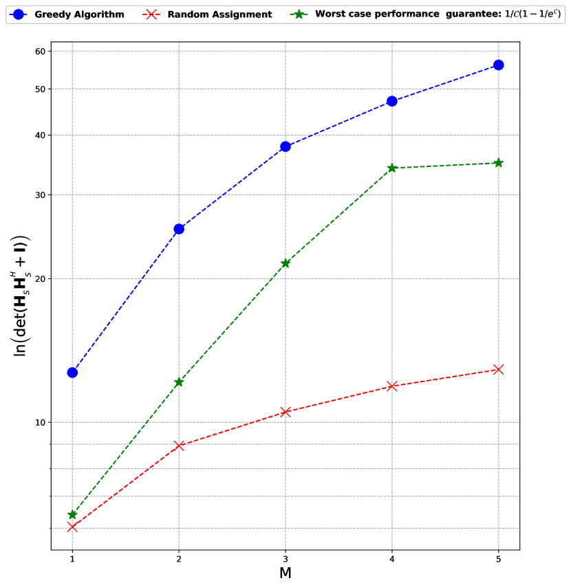
Fig. 2: The value of cost function of (3) plotted against the increasing number of IRS platforms $M$ that are sequentially placed in the radar coverage area $\mathcal{A}$.

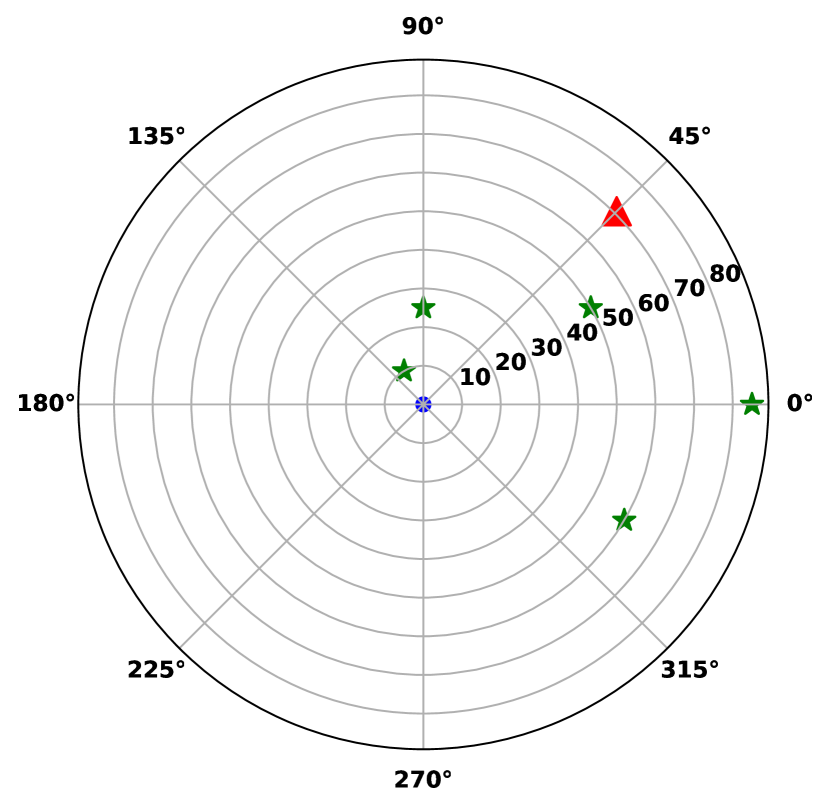
Fig. 3: Optimal placement of $M=5$ IRS platforms (green star) to illuminate the target (red triangle). The radar (blue circle) is located at the origin.

We employed Algorithm 1 to decide the ranges and azimuth angles $(r_{m},\theta_{ri,m})\in\mathcal{A}$ of $M$ IRS platforms tuned at randomly generated phase-shifts comprised in $\bm{\Phi}_{m}$, for $m\in\{1,\ldots,M\}$. Fig. 2 compares the optimized MI-based cost function $f(\mathcal{S})$ for different numbers $M$ of deployed IRS platforms with random placement and the worst-case optimality guarantee of the greedy algorithm. In order to compute the worst-case optimality guarantee of the greedy algorithm, we computed the curvature of the submodular objective function defined in (19) through an exhaustive search. Our experiments showed that $c\approx 0.996$. Fig. 3 illustrates the optimal IRS locations in polar coordinates as obtained by Algorithm 1, for $M=5$ IRS platforms.

5 Summary

We considered an IRS-assisted sensing system and optimized the placement of IRS platforms using the recently proposed tools of submodular optimization. We showed that our MI-based design criterion is submodular and monotonic. The greedy algorithm for submodular optimization yields the optimal placement of IRS platforms in the radar coverage area with a constant suboptimality guarantee. The IRS-aided radar with optimized IRS locations outperforms random placement and the theoretical worst-case optimality guarantee of the greedy algorithm.

References

- [1] A. M. Elbir, K. V. Mishra, M. B. Shankar, and S. Chatzinotas, “The rise of intelligent reflecting surfaces in integrated sensing and communications paradigms,” IEEE Network, 2022, in press.
- [2] T. Wei, L. Wu, K. V. Mishra, and M. Shankar, “RIS-aided wideband holographic DFRC,” arXiv preprint arXiv:2305.04602, 2023.
- [3] J. An, C. Xu, D. W. K. Ng, G. C. Alexandropoulos, C. Huang, C. Yuen, and L. Hanzo, “Stacked intelligent metasurfaces for efficient holographic MIMO communications in 6G,” IEEE Journal on Selected Areas in Communications, vol. 41, no. 8, pp. 2380–2396, 2023.
- [4] D. Tyrovolas, S. A. Tegos, E. C. Dimitriadou-Panidou, P. D. Diamantoulakis, C. K. Liaskos, and G. K. Karagiannidis, “Performance analysis of cascaded reconfigurable intelligent surface networks,” IEEE Wireless Communications Letters, vol. 11, no. 9, pp. 1855–1859, 2022.
- [5] F. Wang and A. L. Swindlehurst, “Hybrid RIS-assisted interference mitigation for spectrum sharing,” in IEEE International Conference on Acoustics, Speech and Signal Processing, 2023, pp. 1–5.
- [6] Z. Esmaeilbeig, A. Eamaz, K. V. Mishra, and M. Soltanalian, “Quantized phase-shift design of active IRS for integrated sensing and communications,” in IEEE International Conference on Acoustics, Speech, and Signal Processing Workshops, 2023, pp. 1–5.
- [7] Z. Wang, X. Mu, and Y. Liu, “STARS enabled integrated sensing and communications,” IEEE Transactions on Wireless Communications, vol. 22, no. 10, pp. 6750–6765, 2023.
- [8] T. Wei, L. Wu, K. V. Mishra, and S. M. Bhavani, “Simultaneous active-passive beamformer design in IRS-enabled multi-carrier DFRC system,” in European Signal Processing Conference, 2022, pp. 1007–1011.
- [9] T. Wei, L. Wu, K. V. Mishra, and M. Shankar, “Multi-IRS-aided Doppler-tolerant wideband DFRC system,” IEEE Transactions on Communications, 2023, in press.
- [10] J. A. Hodge, K. V. Mishra, B. M. Sadler, and A. I. Zaghloul, “Index-modulated metasurface transceiver design using reconfigurable intelligent surfaces for 6G wireless networks,” IEEE Journal of Selected Topics in Signal Processing, 2023, in press.
- [11] Z. Esmaeilbeig, K. V. Mishra, and M. Soltanalian, “IRS-aided radar: Enhanced target parameter estimation via intelligent reflecting surfaces,” in IEEE Sensor Array and Multichannel Signal Processing Workshop, 2022, pp. 286–290.
- [12] Z. Esmaeilbeig, A. Eamaz, K. V. Mishra, and M. Soltanalian, “Joint waveform and passive beamformer design in multi-IRS aided radar,” in IEEE International Conference on Acoustics, Speech and Signal Processing, 2023, in press.
- [13] Z. Esmaeilbeig, K. V. Mishra, A. Eamaz, and M. Soltanalian, “Cramér-Rao lower bound optimization for hidden moving target sensing via multi-IRS-aided radar,” IEEE Signal Processing Letters, vol. 29, pp. 2422–2426, 2022.
- [14] Z. Esmaeilbeig, A. Eamaz, K. V. Mishra, and M. Soltanalian, “Moving target detection via multi-IRS-aided OFDM radar,” in IEEE Radar Conference, 2023, pp. 1–6.
- [15] P.-Q. Huang, Y. Zhou, K. Wang, and B.-C. Wang, “Placement optimization for multi-IRS-aided wireless communications: An adaptive differential evolution algorithm,” IEEE Wireless Communications Letters, vol. 11, no. 5, pp. 942–946, 2022.
- [16] S. Zeng, H. Zhang, B. Di, Z. Han, and L. Song, “Reconfigurable intelligent surface (RIS) assisted wireless coverage extension: RIS orientation and location optimization,” IEEE Communications Letters, vol. 25, no. 1, pp. 269–273, 2020.
- [17] G. Stratidakis, S. Droulias, and A. Alexiou, “Optimal position and orientation study of reconfigurable intelligent surfaces in a mobile user environment,” IEEE Transactions on Antennas and Propagation, vol. 70, no. 10, pp. 8863–8871, 2022.
- [18] S. Ghose, D. Mishra, S. P. Maity, and G. C. Alexandropoulos, “RIS reflection and placement optimisation for underlay D2D communications in cognitive cellular networks,” in IEEE International Conference on Acoustics, Speech and Signal Processing, 2023, pp. 1–5.
- [19] K. Ntontin, D. Selimis, A.-A. A. Boulogeorgos, A. Alexandridis, A. Tsolis, V. Vlachodimitropoulos, and F. Lazarakis, “Optimal reconfigurable intelligent surface placement in millimeter-wave communications,” in European Conference on Antennas and Propagation, 2021, pp. 1–5.
- [20] A. Chen, Y. Chen, and Z. Wang, “Reconfigurable intelligent surface deployment for blind zone improvement in mmWave wireless networks,” IEEE Communications Letters, vol. 26, no. 6, pp. 1423–1427, 2022.
- [21] E. Tohidi, S. Haesloop, L. Thiele, and S. Stanczak, “Near-optimal LoS and orientation aware intelligent reflecting surface placement,” arXiv preprint arXiv:2305.03451, 2023.
- [22] F. T. Ulaby, R. K. Moore, and A. K. Fung, Microwave Remote Sensing: Active and Passive. Volume 1 - Microwave Remote Sensing Fundamentals and Radiometry. Artech House, 1981.
- [23] M. M. Naghsh, M. Modarres-Hashemi, S. ShahbazPanahi, M. Soltanalian, and P. Stoica, “Majorization-minimization technique for multi-static radar code design,” in European Signal Processing Conference, 2013, pp. 1–5.
- [24] M. M. Naghsh, M. Modarres-Hashemi, A. Sheikhi, M. Soltanalian, and P. Stoica, “Unimodular code design for MIMO radar using bhattacharyya distance,” in IEEE International Conference on Acoustics, Speech and Signal Processing, 2014, pp. 5282–5286.
- [25] M. Alaee-Kerahroodi, M. Soltanalian, P. Babu, and M. R. B. Shankar, Signal design for modern radar systems. Artech House, 2022.
- [26] J. Liu, K. V. Mishra, and M. Saquib, “Co-designing statistical MIMO radar and in-band full-duplex multi-user MIMO communications,” arXiv preprint arXiv:2006.14774, 2020.
- [27] S. Joshi and S. Boyd, “Sensor selection via convex optimization,” IEEE Transactions on Signal Processing, vol. 57, no. 2, pp. 451–462, 2009.
- [28] H. Godrich, A. P. Petropulu, and H. V. Poor, “Sensor selection in distributed multiple-radar architectures for localization: A knapsack problem formulation,” IEEE Transactions on Signal Processing, vol. 60, no. 1, pp. 247–260, 2012.
- [29] K. V. Mishra, A. M. Elbir, and K. Ichige, “Sparse array design for direction finding using deep learning,” in Sparse Arrays for Radar, Sonar, and Communications. Wiley-IEEE Press, 2023, in press.
- [30] G. Shulkind, S. Jegelka, and G. W. Wornell, “Sensor array design through submodular optimization,” IEEE Transactions on Information Theory, vol. 65, no. 1, pp. 664–675, 2018.
- [31] E. Tohidi, R. Amiri, M. Coutino, D. Gesbert, G. Leus, and A. Karbasi, “Submodularity in action: From machine learning to signal processing applications,” IEEE Signal Processing Magazine, vol. 37, no. 5, pp. 120–133, 2020.
- [32] K. V. Mishra and Y. C. Eldar, “Sub-Nyquist channel estimation over IEEE 802.11ad link,” in IEEE International Conference on Sampling Theory and Applications, 2017, pp. 355–359.
- [33] T. M. Cover, Elements of information theory. John Wiley & Sons, 1999.
- [34] U. Feige, “A threshold of ln for approximating set cover,” Journal of the ACM, vol. 45, no. 4, pp. 634–652, 1998.
- [35] M. Sviridenko, J. Vondrák, and J. Ward, “Optimal approximation for submodular and supermodular optimization with bounded curvature,” Mathematics of Operations Research, vol. 42, no. 4, pp. 1197–1218, 2017.