CMDA: a tool for Continuous Monitoring Data Analysis

Abstract

Over the last few years, with the growth of time-series collecting and storing, there has been a great demand for tools and software for temporal data engineering and modeling. This paper presents a generic workflow for time series data research, including temporal data importing, preprocessing, and feature extraction. This framework is developed and built as a robust and easy-to-use Python package, called CMDA, with a modular structure that offers tools to prepare raw data, allowing both scientists and non-experts to analyze various temporal data structures.

Keywords Time Series  $\cdot$ Monitoring Data  $\cdot$ Feature Extraction  $\cdot$ Preprocessing

1 Introduction

Data generation and collection in real-time is more ubiquitous than ever due to technological progress in sensors, transmission, and data storage. This has resulted in enormous datasets, namely Big Data, in various fields such as engineering, medical, physical, and social sciences. While effective modeling and simulation of such datasets can offer rich information for interpretation, prediction, monitoring, training, and decision making, their scope and complexity create significant design and implementation issues [3].
For instance, in the healthcare systems, continuous monitoring data has developed into a breakthrough for health diagnosis, subsequent treatment, and proactive health tracking [1]. The recent advancements in wearable technology and monitoring systems have offered unseen opportunities for learning mechanisms of biomedical processes from temporal data as they provide data on physiological occurrences that indicate an individual’s health and comfort. However, it must be taken into account that, the analysis of continuous monitoring data is highly affected by data quality issues and even complex monitoring devices can monitor only a small subset of medical parameters involved in the process under consideration. Furthermore, the required analysis strategies for monitoring data vary significantly between monitoring a few parameters assessed on dense sampling rates (e.g., ECG, EEG, or glucose data) and monitoring several parameters over hours with low sampling frequency, as in ICU. On account of this, there is a significant demand for robust and easy-to-implement tools to facilitate continuous data wrangling and feature engineering. In order to address this, we introduce the CMDA package to provide a comprehensive monitoring data analysis workflow. CMDA, developed and built as a Python package, is a standard framework for time series data research, including temporal data importing, preprocessing, and feature extraction.

2 Structure

A general workflow for continuous data analysis consists of four steps: importing the time-series records, preprocessing (missing value imputation and denoising), feature extraction, and model creation.
Initially, continuous data is imported from various sources. Second, the imported data is preprocessed based on their quality to verify that only the relevant data reach the subsequent steps. This can involve eliminating irrelevant artifacts from the data (via filtering and outlier removal techniques) and windowing signals to a set of time bins. In the step before modeling, features relevant to a particular problem are derived from filtered data.
Feature extraction or engineering uncovers the masked characteristics of raw temporal data. In other words, it can be described as a set of features corresponding to the signal’s specific form or pattern. Additionally, feature extraction is generally a procedure that reduces the dimensionality of an input signal or compresses its data and thus reduces the number of resources needed for analysis. Performing extraction of descriptors on a raw signal would result in low dimensional data that could accurately elaborate the input raw data and aid in developing a practical and interpretable input for machine learning tasks.
CMDA offers a set of tools for the mentioned steps in a modular structure, allowing users to use modules individually as part of another project, depending on the application. Nevertheless, the whole process can be integrated into a pipeline, which can be executed in a parallel fashion. Figure 1 depicts the components of the feature engineering pipeline. The other noteworthy attribute of CMDA is that besides the built-in feature functions, user-defined functions can be added easily to the pipeline, which enables more adaptable use of the feature engineering module. A detailed description of the package architecture, including the data importing modules and feature extraction modules, as well as the list of the built-in feature functions, can be found in the next section along with tutorials in appendix A.

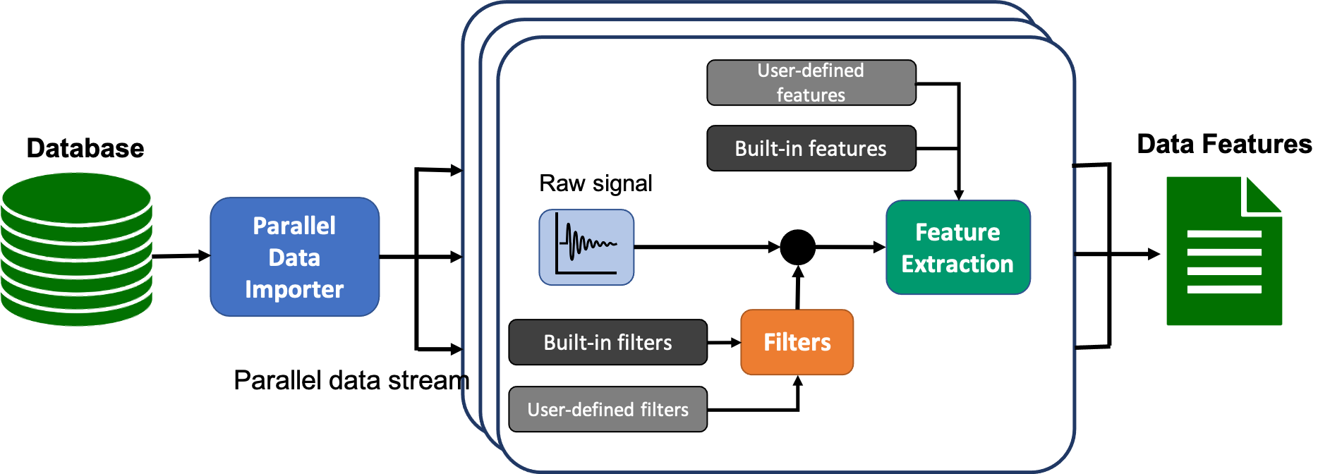
Figure 1: Illustration of the CMDA workflow. The pipeline consists of three components. In the feature engineering stage, data records can be imported into the pipeline either consecutively or in parallel. Once filters are applied (if needed) and features are extracted, these data features are saved to a file. The features can be used later for any ML task.

3 Architecture

3.1 Data Importer Module

Data importer ( cmda.import_data), the first component in the pipeline, offers tools for loading multiple CSV files from a server or local disk into the python coding environment ( cmda.import_data.ImportCSV). It should be taken into account that the CSV files must contain signals as columns and temporal instances as rows.
The importer module also supports importing DAT files directly from Physionet databases ( cmda.import_data.ImportWFDB) using WFDB package APIs [11]. Physionet, a funded project by the National Institutes of Health, is a vast and growing archive of digital recordings of physiologic signals and corresponding data for the use of medical research [4].
The importer functions can save computation time by parallelizing the data loading process. Moreover, in the case of a very long time series, if windowing or segmentation is required, a rolling window importer function performs the time binning with a defined window length and step size. It distributes the importing process for each window across available nodes in parallel. Users can access the rolling window via cmda.import_data.RollingWindowCSV. The library offers modules for importing continuous data from both local disk and Physionet databases.

3.2 Preprocessing Module

cmda.preprocessing.Filters is a tool for applying different filters and outlier removal functions on a numeric signal. Users can select from several built-in filters using a dynamic attribute of the Filters object, .add, which provides access to the following functions:

Table 1: Built-in preprocessing features

Feature function	Feature	Description
rm_outlier	Remove Outlier	Removing outliers based on a $low$ and $high$ threshold
rm_outliers_quantile	Remove Quantiles	Removing the values in an array based on $low$ and $high$ defined quantiles
butter_filter	Butterworth Filter	A predesigned Butterworth filter that can be used as a band-pass denoisng tool
interpolate	Interpolation	A $linear$ or $cubic$ interpolation tool that can be used for imputing missing values in an array

Moreover, users can easily add their own defined filters to the Filters object instance using .udf.add. This functionality makes it possible to tailor the filters based on the application.

3.3 Feature Extraction Module

cmda.feature_extraction.Features is a tool for extracting multiple features from a numeric time series array. This library provides several ready-to-use built-in time domain, spectral domain, nonlinear, and wavelet features that can be selected and added to a Features object instance via .add function.
Additionally, users can define and add their own functions to the Features object instance using .udf.add. The available built-in functions in the current version of the package are described in the following sections.

3.3.1 Time-domain Features

Time-domain features describe signals over a span of time. The list of all built-in time-domain features is shown in Table LABEL:tab:tdf. These functions are defined using the NumPy [5] package.

Table 2: Built-in time-domain features

Feature function	Feature	Description
mean	Mean	Arithmetic mean of an array elements
max	Maximum	Maximum value of an array elements
min	Minimum	Minimum value of an array elements
median	Median	Median value of an array elements
std	Standard Deviation	Standard deviation of an array elements
skewness	Skewness	Skewness of an array elements
kurtosis	Kurtosis	Kurtosis of an array elements
p2p	Peak-to-Peak	Peak to peak difference (maximum - minimum values) of an array elements
rms	Root Means Square	Root means square of an array elements
zcr	Zero Crossing Rate	The rate at which an 1-D array changes from positive to zero to negative or from negative to zero to positive
mad	Mean Absolute Deviation	The median of the absolute deviations an array. Also called median of slopes
mns	Mean Slope	The mean differences of an array

3.3.2 Frequency-domain Features

Frequency-domain features, extracted from the Fourier transform of a signal, describe its characteristics in the frequency domain. The list of all built-in frequency-domain features is shown in Table LABEL:tab:fdf. These functions are defined using the NumPy [5] and SciPy [10] packages.

Table 3: Built-in frequency-domain features

Feature function	Feature	Description
periodogram	Periodogram	The power spectrum density of an array [8]
welch	Welch Periodogram	The power spectrum density of an array computed using welch method.
mnf	Mean frequency	The center of the distribution of power across frequencies. It is calculated as the sum of product of the power spectrum and the frequency divided by the total sum of the power spectrum [8].
mdf	Median frequency	The frequency at which the power spectrum is divided into two parts with equal powers [8].
vcf	Variance of central frequency	The variance of power spectrum amplitudes from its mean frequency [8].
peaks	Peak Frequency	The frequency at which the maximum of power spectrum occurs [8].
psr	Power spectrum ratio	The ratio between the energy around the maximum value of the power spectrum and the whole energy of the power spectrum [8].
band_power	Band Power	The power spectral density in a specified frequency band.
band_std	Band Standard Deviation	The power spectral standard deviation in a specified frequency band.
band_mnf	Band Mean Frequency	The mean frequency of a specified frequency band.
band_mdf	Band Median Frequency	The median frequency of a specified frequency band.

3.3.3 Entropy Features

Shannon entropy and its derivations are methods for estimating the complexity of dynamic systems. Table LABEL:tab:entropy shows the available entropy built-in functions in CMDA.

Table 4: Built-in entropy features

Feature function	Feature	Description
entropy	Shannon Entropy	A technique for estimating the irregularity in temporal data [9]
sample_entropy	Sample Entropy	A technique for estimating the complexity of dynamic physiological systems based on the existence of patterns [9]
perm_entropy	Permutation Entropy	A derivation of Shannon entropy, used to assess the complexity of time series data, proposed by Bandt[2]. It quantifies the complexity of a system based on similar ordinal patterns.
spectral_entropy	Spectral Entropy	A measure of the uniformity of a power spectrum frequency distribution [7].

3.3.4 Wavelet Features

The wavelet transform provides a significant method for joint time-frequency feature extraction. It was developed to deal with non-stationary signals. The wavelet transform is classified as discrete or continuous. Computing wavelet coefficients at every feasible scale can be time-consuming and produce a large amount of data. As a result, the DWT (Discrete wavelet transform) is extensively used. However, it suffers from the downsample resolution of DWT at higher decomposition levels and destroys the time invariance property. The Stationary wavelet transform (SWT) [6] is a wavelet transform algorithm designed to overcome the downsample problem of DWT and preserves the time information. CMDA offers a built-in swt_features function that returns both time-domain and frequency-domain coefficients from decomposition levels. The following parameters can be given to the function:

• Mean Frequency (mnf)

• Power Spectrum Ratio (psr)

• Peak Frequency (peak)

• Median Absolute Deviation (mds)

• Mean Slope (mns)

• Shannon Entropy (see)

• Permutation Entropy (perm-ent)

• Normalized Energy (nse)

The explanation of each parameter can be found in Tables LABEL:tab:tdf, LABEL:tab:fdf, and LABEL:tab:entropy.

3.4 Feature Engineering Pipeline

cmda.pipeline.Pipeline is a tool for importing, pre-processing and feature extraction of multiple records (files) in an automated manner.
Users must create an importer object instance using cmda.import_data, a feature object instance using cmda.preprocessing.Features, and, if needed, a filter object instance with cmda.preprocessing.Filters. They must then feed these instances into the pipeline. The process can be executed either consecutively or in parallel using the .run function.

4 Discussions

The CMDA Python package is designed to facilitate a monitoring data analysis workflow, with functions ranging from reading multiple datasets to denoising and feature extraction. Its modular design allows for implementation across various applications and supports the integration of user-defined components. The package provides a fast and straightforward workflow with minimum coding requirements, making it feasible for the researchers to prepare ready-to-analyze extensive monitoring datasets before applying any sophisticated strategy. In the future development of CMDA, we aim to add more built-in features and pre-processing functions to cover broader applications. In addition, embedding unsupervised feature engineering methods such as deep autoencoders and signal to image transformation is another objective of the package expansion. Until then, we hope CMDA enhances healthcare data expertise by setting a standard for monitoring data analysis.

5 Software Availability

The CMDA toolkit is freely accessible as open-source on GitHub. The software can be accessed and downloaded from:

www.github.com/JRC-COMBINE/cmda

A README file within the repository provides insights into the software’s setup process, required dependencies, and instructions for use. For any concerns or queries, please use the "Issues" section of the GitHub repository. Community input and contributions to improve the toolkit are highly welcomed.

Appendix A Examples

A.1 Feature Object

cmda.feature_extraction.Features is a tool for extracting multiple features at the same time from a numeric signal x. One can select from a wide variety of built-in features, as well as adding user-defined features. This functionality makes it possible to tailor the features based on the application. The following subsections show examples of time domain, frequency domain, and user-defined feature extraction.

A.1.1 Import the data

We start by using sample data contains an ECG signal and ABP (Arterial Blood Pressure) signal with a length of 10 seconds and 125 Hz sampling rate. The toy data can be accessed from cmda.data.ecg_abp_sample.

⬇

1import numpy as np

2import matplotlib.pyplot as plt

3

4from cmda.data import ecg_apb_sample

5

6data = ecg_apb_sample()

7

8ecg = data["ECG"]

9abp = data["ABP"]

10

11fs = 125

12t = np.linspace(1, 1 / fs, len(ecg))

13fig, (ax1, ax2) = plt.subplots(2, sharex=True)

14ax1.plot(t, ecg)

15ax1.set_ylabel("ECG [mV]")

16ax2.plot(t, abp, c="red")

17ax2.set_ylabel("ABP [mmHg]")

18ax2.set_xlabel("Time [seconds]")

19plt.show()

Listing 1: Importing a sample data

Output:

Figure 2: Imported ECG and ABP sample signals

A.1.2 Time-domain feature extraction

In this example, we extract some built-in time-domain features of the ABP signal. To start, we must call the cmda.feature_extraction.Features object and add the desired features using the add function.
After adding the features, we apply the transform function to the signal and get the features. The transform function returns the extracted features as a python dictionary.

⬇

1from cmda.feature_extraction import Features

2from cmda.data import ecg_apb_sample

3

4data = ecg_apb_sample()

5x = data["ABP"]

6

7feature = Features()

8

9# add built-in time-domain features

10feature.add.mean()

11feature.add.max()

12feature.add.min()

13feature.add.median()

14feature.add.skewness()

15feature.add.kurtosis()

16feature.add.std()

17feature.add.p2p()

18feature.add.zcr(center=True)

19

20feature.transform(x=x, fs=125)

Listing 2: Time-domain feature extraction

Output:

⬇

1{’mean’: 72.385,

2 ’max’: 107.03125,

3 ’min’: 53.125,

4 ’median’: 69.53125,

5 ’skewness’: 0.9154627781784881,

6 ’kurtosis’: -0.15299373030467667,

7 ’std’: 13.268216310510619,

8 ’p2p’: 53.90625,

9 ’zcr’: 42}

Listing 3: Time-domain feature extraction output

A.1.3 Frequency-domain feature extraction

In this part, we extract some built-in frequency-domain features of the ECG signal. Similar to the previous example, we call the cmda.feature_extraction.Features object, and append the desired features using the add function.
Using the transform function returns the extracted features as a python dictionary.

⬇

1from cmda.feature_extraction import Features

2from cmda.data import ecg_apb_sample

3

4data = ecg_apb_sample()

5x = data["ECG"]

6

7feature = Features()

8

9# add frequency-domain built-in features

10feature.add.mnf(spectrum="ps")

11feature.add.mdf(spectrum="ps")

12feature.add.stdf(spectrum="ps")

13feature.add.psr(spectrum="welch", int_limit_ratio=0.01)

14feature.add.peaks(spectrum="welch", n_peaks=1, height=True, width=True)

15feature.add.band_power(spectrum="ps", low=1, high=7)

16feature.add.band_mnf(spectrum="ps", low=1, high=7)

17

18feature.transform(x=x, fs=125)

Listing 4: Frequency-domain feature extraction

Output:

⬇

1{’mnf’: 9.857968968908676,

2 ’mdf’: 9.0,

3 ’stdf’: 6.657686374206612,

4 ’psr_0.01’: 0.1086823980353686,

5 ’peak_freq_1’: 3.90625,

6 ’peak_height_1’: 0.0009058970155242925,

7 ’peak_width_1’: 4.386465062242469,

8 ’power_[1,7]Hz’: 0.3921784430303598,

9 ’mnf_[1,7]Hz’: 4.277888519896743}

Listing 5: Frequency-domain feature extraction output

A.1.4 User-defined feature extraction

In this section, we derive some features, including a user-defined feature from the ABP signal. Similar to the previous example, we call the cmda.feature_extraction.Features object, Define the feature and add them to the feature object, using add_udf function. The transform function returns the extracted features as a python dictionary.

⬇

1import numpy as np

2from cmda.feature_extraction import Features

3from cmda.data import ecg_apb_sample

4

5data = ecg_apb_sample()

6x = data["ABP"]

7

8# Define the feature

9# Please take note, that the output must be a dictionary

10# ,where the keys are the extracted features

11def quantile(x,low = 0.1,high =0.9):

12 q_low = np.quantile(x,q=low)

13 q_high = np.quantile(x,q=high)

14

15 res = {"q_low":q_low, "q_high":q_high}

16 return res

17

18

19# Call the Feature object

20feature = Features()

21

22# add built-in features

23feature.add.mean()

24feature.add.max()

25feature.add.zcr(center=True)

26feature.add.mnf(spectrum="ps")

27

28# add user-defined feature

29feature.udf.add(quantile)

30

31feature.transform(x=x, fs=125)

Listing 6: User-defined feature extraction

Output:

⬇

1{’mean’: 72.385,

2 ’max’: 107.03125,

3 ’zcr’: 42,

4 ’mnf’: 2.0056974184541025,

5 ’q_low’: -13.79125,

6 ’q_high’: 23.70875}

Listing 7: User-defined feature extraction output

A.2 Multivariate Feature Extraction

In this tutorial, we show how to extract features from a multivariate signal. In the first example, we extract similar features from all the variables, and in the second part, we show how to extract different features from each variable. Please read A.1 on how to create a feature object first. We use the same data as used in the Feature Object tutorial (A.1). The data contain two signals (ECG, ABP) with a sampling frequency = 500.

A.2.1 Feature extraction with one feature object

To extract features from a dataset, we use cmda.feature_extraction.extract_features function. First, we create a feature object with cmda.feature_ectraction.Features.

⬇

1from cmda.feature_extraction import Features

2from cmda.feature_extraction import extract_features

3from cmda.data import ecg_apb_sample

4

5# load the data

6data = ecg_apb_sample()

7

8# Create the feeature object

9features = Features()

10

11# Add built-in features

12features.add.std()

13features.add.mnf()

14features.add.stdf()

15

16# extract eatures

17res = extract_features(data=data, feature_obj=features)

18

19print(res)

Listing 8: Multivariate feature extraction using one feature object

Output:

⬇

1{’ECG_std’: 0.0912508348533301,

2 ’ECG_mnf’: 0.0788637517512694,

3 ’ECG_stdf’: 0.053261490993652905,

4 ’ABP_std’: 13.268216310510619,

5 ’ABP_mnf’: 0.01604557934763282,

6 ’ABP_stdf’: 0.012480758701313835}

A.2.2 Feature extraction with multiple feature objects

In various real applications, extracting similar features from different signals may lead to wrong data compression and unnecessary information. To avoid that, we show how to create and apply signal-specific feature objects.

⬇

1from cmda.feature_extraction import Features

2from cmda.feature_extraction import extract_features

3from cmda.data import ecg_apb_sample

4

5# load the data

6data = ecg_apb_sample()

7

8# Create the feature object for ECG signal

9ecg_features = Features()

10

11# Add built-in features

12ecg_features.add.mnf()

13ecg_features.add.stdf()

14

15

16# Create the feature object for ECG signal

17abp_features = Features()

18

19# Add built-in features

20abp_features.add.mean()

21abp_features.add.std()

22abp_features.add.max()

23abp_features.add.min()

24

25# Create the feature object as a dict

26features = {’ECG’:ecg_features, ’ABP’:abp_features}

27

28# extract eatures

29res = extract_features(data=data, feature_obj=features)

30

31print(res)

Listing 9: Multivariate feature extraction using one feature object

Output:

⬇

1{’ECG_mnf’: 0.0788637517512694,

2 ’ECG_stdf’: 0.053261490993652905,

3 ’ABP_mean’: 72.385,

4 ’ABP_std’: 13.268216310510619,

5 ’ABP_max’: 107.03125,

6 ’ABP_min’: 53.125}

A.3 Feature Extraction Pipeline

This tutorial shows how to implement cmda.pipeline.Pipeline to extract features from a Physionet WFDB. We extract features from the ECGRDVQ database. The database contains 5232 extracted 10-second standard 12 lead ECG segments. The meta-data of the database ( ecgrdvq_metadata), which is a dictionary consisting of the record names record_name and their corresponding public directories public_dir, is available in cmda.data.wfdb. The pipeline includes importing the data, applying filters to the records, and feature extraction from records. To import the data from Physionet WFDB, we use the cmda.read_data.ReadWFDB. We create the filtering object by cmda.filter.Filters and create the feature object by cmda.feature_extraction.Features. A detailed tutorial on creating feature objects can be found in A.1.

⬇

1from cmda.data.wfdb import ecgrdvq_metadata

2from cmda.read_data import ReadWFDB

3from cmda.preprocessing import Filters

4from cmda.feature_extraction import Features

5from cmda.pipeline import Pipeline

6

7# Load the meta-data

8metadata = ecgrdvq_metadata()

9

10# get the record names and their corresponding public directories

11record_names = metadata[’record_name’]

12public_dir = metadata[’public_dir’]

13

14# Build the importer object using ReadWFDB

15# Set the channels to ["II",’V1’] to import these channels exclusively.

16importer = ReadWFDB(record_names=record_names, public_dir=public_dir, channels=[’II’,’V1’])

17

18# Create the filter object and add a buuterworth low-pass filter

19filter_obj = Filters()

20filter_obj.add.butter_filter(cutoff=60, btype="lowpass")

21

22# Create the feature object

23feature_obj = Features()

24feature_obj.add.mnf()

25feature_obj.add.mdf()

26feature_obj.add.psr()

27feature_obj.add.stdf()

28feature_obj.add.peaks(n_peaks=1,spectrum=’welch’,height=False,width=False,nperseg=512)

29feature_obj.add.band_power(low=0.6, high=2,spectrum=’welch’)

30feature_obj.add.band_power(low=2, high=4,spectrum=’welch’)

31feature_obj.add.band_power(low=4, high=6,spectrum=’welch’)

32feature_obj.add.band_power(low=6, high=10,spectrum=’welch’)

33feature_obj.add.band_power(low=10, high=15,spectrum=’welch’)

34feature_obj.add.band_power(low=15, high=30,spectrum=’welch’)

35

36# Build the pipeline

37ecgrdvq_pipeline = Pipeline(importer=importer,features=feature_obj, filters=filter_obj)

38

39# Run the pipeline

40# Set the dataframe_output to True, to get the extracted as a Pandas dataframe

41# n_jobs set the number of cpu cores for parallel feature extraction

42res = ecgrdvq_pipeline.run(n_jobs=4, dataframe_output = True)

Listing 10: Multivariate feature extraction using one feature object

Output:

⬇

1Running the pipeline on 5232 instances...

2

3100% [|||||||||||||||] 5232/5232 [00:05<00:00, 2.23it/s]

4

5finished!

The required time for parallel running the above pipeline was around 2640 seconds for a PC with a 3,5 GHz Dual-Core Intel Core i7 processor and 16 GB 2133 MHz LPDDR3 memory. The process included retrieving the data from Physionet data servers too.

References

- [1] Y. Athavale and S. Krishnan. Biosignal monitoring using wearables: Observations and opportunities. Biomedical Signal Processing and Control, 38:22–33, Sept. 2017.
- [2] C. Bandt and B. Pompe. Permutation Entropy: A Natural Complexity Measure for Time Series. Physical Review Letters, 88(17):174102, Apr. 2002.
- [3] H. Fröhlich, R. Balling, N. Beerenwinkel, O. Kohlbacher, S. Kumar, T. Lengauer, M. H. Maathuis, Y. Moreau, S. A. Murphy, T. M. Przytycka, M. Rebhan, H. Röst, A. Schuppert, M. Schwab, R. Spang, D. Stekhoven, J. Sun, A. Weber, D. Ziemek, and B. Zupan. From hype to reality: data science enabling personalized medicine. BMC Medicine, 16(1):150, Dec. 2018.
- [4] A. L. Goldberger, L. A. N. Amaral, L. Glass, J. M. Hausdorff, P. C. Ivanov, R. G. Mark, J. E. Mietus, G. B. Moody, C.-K. Peng, and H. E. Stanley. PhysioBank, PhysioToolkit, and PhysioNet: Components of a New Research Resource for Complex Physiologic Signals. Circulation, 101(23), June 2000.
- [5] C. R. Harris, K. J. Millman, S. J. v. d. Walt, R. Gommers, P. Virtanen, D. Cournapeau, E. Wieser, J. Taylor, S. Berg, N. J. Smith, R. Kern, M. Picus, S. Hoyer, M. H. v. Kerkwijk, M. Brett, A. Haldane, J. F. d. Río, M. Wiebe, P. Peterson, P. Gérard-Marchant, K. Sheppard, T. Reddy, W. Weckesser, H. Abbasi, C. Gohlke, and T. E. Oliphant. Array programming with NumPy. Nature, 585(7825):357–362, Sept. 2020. Publisher: Springer Science and Business Media LLC.
- [6] M. Holschneider, R. Kronland-Martinet, J. Morlet, and P. Tchamitchian. A Real-Time Algorithm for Signal Analysis with the Help of the Wavelet Transform. In J.-M. Combes, A. Grossmann, and P. Tchamitchian, editors, Wavelets, pages 286–297. Springer Berlin Heidelberg, Berlin, Heidelberg, 1990. Series Title: inverse problems and theoretical imaging.
- [7] Y. N. Pan, J. Chen, and X. L. Li. Spectral entropy: A complementary index for rolling element bearing performance degradation assessment. Proceedings of the Institution of Mechanical Engineers, Part C: Journal of Mechanical Engineering Science, 223(5):1223–1231, May 2009.
- [8] A. Phinyomark, S. Thongpanja, H. Hu, P. Phukpattaranont, and C. Limsakul. The Usefulness of Mean and Median Frequencies in Electromyography Analysis. In G. R. Naik, editor, Computational Intelligence in Electromyography Analysis - A Perspective on Current Applications and Future Challenges. InTech, Oct. 2012.
- [9] J. S. Richman and J. R. Moorman. Physiological time-series analysis using approximate entropy and sample entropy. American Journal of Physiology-Heart and Circulatory Physiology, 278(6):H2039–H2049, June 2000.
- [10] P. Virtanen, R. Gommers, T. E. Oliphant, M. Haberland, T. Reddy, D. Cournapeau, E. Burovski, P. Peterson, W. Weckesser, J. Bright, S. J. van der Walt, M. Brett, J. Wilson, K. J. Millman, N. Mayorov, A. R. J. Nelson, E. Jones, R. Kern, E. Larson, C. J. Carey, İ. Polat, Y. Feng, E. W. Moore, J. VanderPlas, D. Laxalde, J. Perktold, R. Cimrman, I. Henriksen, E. A. Quintero, C. R. Harris, A. M. Archibald, A. H. Ribeiro, F. Pedregosa, P. van Mulbregt, and SciPy 1.0 Contributors. SciPy 1.0: Fundamental Algorithms for Scientific Computing in Python. Nature Methods, 17:261–272, 2020.
- [11] C. Xie, L. McCullum, A. Johnson, T. Pollard, B. Gow, and B. Moody. Waveform Database Software Package (WFDB) for Python.