[1]Illia Horenko

[1]Chair for Mathematics of AI, Faculty of Mathematics, RPTU Kaiserslautern-Landau, Gottlieb-Daimler-Str. 48, Kaiserslautern, 67663, Germany

On existence, uniqueness and scalability of adversarial robustness and control measures for AI classifiers

Abstract

Simply-verifiable mathematical conditions for existence, uniqueness and explicit analytical computation of minimal adversarial paths (MAP) and minimal adversarial distances (MAD) for (locally) uniquely-invertible classifiers, for generalized linear models (GLM), and for entropic AI (EAI) are formulated and proven. Practical computation of MAP and MAD, their comparison and interpretations for various classes of AI tools (for neuronal networks, boosted random forests, GLM and EAI) are demonstrated on the common synthetic benchmarks: on a double Swiss roll spiral and its extensions, as well as on the two biomedical data problems (for the health insurance claim predictions, and for the heart attack lethality classification). On biomedical applications it is demonstrated how MAP provides unique minimal patient-specific risk-mitigating interventions in the predefined subsets of accessible control variables.

Understanding and measuring accountability and robustness of rapidly-developing Artificial Intelligence tools (AI) is recently moving to the center of AI research. As formulated in the seminal paper featuring the sparks of artificial general intelligence that are shown by Chat GPT-4, in the last sentence of their paper the Microsoft Research team says that "elucidating the nature and mechanisms of AI systems such as GPT-4 is a formidable challenge that has suddenly become important and urgent" [1]. Importance of getting a better understanding of the nature and mechanisms of the AI is especially underlined by the multiple very spectacular recent examples of the so-called adversarial attacks on AI tools, when very small changes in the input data - practically non-perceptable for humans - could be used for a complete corruption of the AI classification outcomes [2]. Similar adversarial attacks were recently shown to help designing strategies that beat the superhuman AlphaGo AIs - showcasing significant problems with robustness of such AI tools [3]. Also very recently, mathematical approaches provided decisive insights into these problems - allowing a systematic development of efficient adversarial algorithms [2, 4]. For example, it was demonstrated that one can use the same mathematical concepts, like the gradient descent method (normally used in the training of AI tools), to find the adversarial attacks as solutions of numerical optimization problems. In the so-called untargeted attacks, for a given feature vector $X$ with a label $L$ and an AI classifier with the trained class affiliation probability function $\mathbb{P}_{L}(X)$, one is trying to find the adversarial vector $X^{*}$ that is as close as possible to the given vector $X$ in terms of some distance measure $\text{dist}(X,X^{*})$ and such that $\mathbb{P}_{L^{*}}(X^{*})$ is attaining its maximal value for $L^{*}\neq L$ [2, 4]. However, mathematical properties like existence, uniqueness and numerical scalability of adversarial problems solutions - necessary for validity and feasibility of these mathematical methods - remain a major bottleneck, requiring a fulfilment of very strong assumptions like strong Lipschitz-convexity of the class affiliation probability function $\mathbb{P}_{L}(X)$ (see, e.g., eq. 4 and Theorem 1 in [4]). As can be seen from the contour lines of $\mathbb{P}_{L}(X)$ in panels A-F of Fig. 1 below, even for the most basic AI benchmarks - like for a very common double-spiral Swiss roll example [5] - class affiliation probability functions are non-convex.

As will be demonstrated below on biomedical examples, in many AI applications only a subset $d_{a}\subseteq\left\{1,\dots,D\right\}$ of the $D$ degrees of freedom of the feature vector $X$ is available for changes and control in the adversarial attack - and there is a complementary feature subset $d_{na}=\left\{1,\dots,D\right\}\setminus d_{a}$ (e.g., an age or a sex of the patient) that are not accessible for such an attack or control. For a given feature vector $X$ with label $L$, accessible features subset $d_{a}$, and a class affiliation probability function $\mathbb{P}_{L}(X)$ , in the following we will first consider finding minimal adversarial path (MAP) from $X$ to (a priori unknown) $X^{*}$ as a solution of the following optimization problem:

$$X^{*} = \arg\min_{\tilde{X}}\text{dist}(X,\tilde{X}),$$ (1)

such that $$\mathbb{P}_{L}(X)-\mathbb{P}_{L}(\tilde{X})=\delta>0,$$ (2)

$$\tilde{X}_{i\in d_{na}} = {X}_{i\in d_{na}}.$$ (3)

The minimal adversarial distance measure $MAD_{L}(X,\delta)=\text{dist}(X,X^{*})$ will then be defined as a length of this path. Let us first assume that the function $\mathbb{P}_{L}(\cdot)$ is (locally) uniquely-invertible in some neighbourhood $S(X)$ of $X$, i.e., that there exists an inverse function $\mathbb{P}^{\dagger}_{L,S(X)}(\cdot)$ such that for any $X$ and $Y$ from $S(X)$ it is fulfilled that $Y=\mathbb{P}^{\dagger}_{L,S(X)}(\mathbb{P}_{L}(X))$ if and only if $X=Y$. This is a very strong assumption - but we start with it to illustrate the underlying idea and to elaborate on this idea later in order to soften this assumption. It is easy to verify that adopting this unique-invertibility assumption, rearranging terms in (2) and applying the local inverse $\mathbb{P}^{\dagger}_{L,S(X)}(\cdot)$ to both sides of the resulting equality (assuming that $\tilde{X}\in S(X)$) we can equivalently transform (2) to the equality that is linear in $\tilde{X}$. Then, problem (1-3) can be rewritten as a convex constrained regularization problem:

$$X_{\epsilon,\delta}^{*} = \arg\min_{\tilde{X}}\left[\text{dist}(X,\tilde{X})+\epsilon^{2}\left(\tilde{X}-\mathbb{P}^{\dagger}_{L,S(X)}\left(\mathbb{P}_{L}\left(X\right)-\delta\right)\right)^{2}\right],$$ (4)

$$\tilde{X}_{i\in d_{na}} = {X}_{i\in d_{na}}\text{ and }\tilde{X}\in S(X).$$ (5)

Increasing the scalar regularization parameter $\epsilon^{2}$ results in imposing more "weight" on a "soft" fulfilment of the equality constraint (2). This idea constitutes a core of the "penalty method" for solving equality-constrained optimization problems [6]. Under some conditions - summarized in the following Theorem 1 - this regularized problem (4-5) can be solved explicitly, resulting in the closed-form analytical solution for $X_{\epsilon,\delta}^{*}$.

Theorem 1.

Let $X,\tilde{X}\in\mathbf{R}^{D}$, dist$(X,\tilde{X})=\|X-\tilde{X}\|_{2}^{2}$, and $\mathbb{P}_{L}(\cdot)$ be a (locally) uniquely-invertible classifier function in the neighbourhood $S(X)$ of $X$. Then, for any $\delta\geq 0$ and $\epsilon$ problem (4) has a unique solution $X_{\epsilon,\delta}^{*}$:

$$\left\{X_{\epsilon,\delta}^{*}\right\}_{i\in d_{a}} = \frac{\left\{X\right\}_{i\in d_{a}}+\epsilon^{2}\left\{C(\delta,X)\right\}_{i\in d_{a}}}{1+\epsilon^{2}},$$

$$\left\{X_{\epsilon,\delta}^{*}\right\}_{i\in d_{na}} = \left\{X\right\}_{i\in d_{na}},$$ (6)

if $X_{\epsilon,\delta}^{*}\in S(X)$, where $C(\delta,X)=\mathbb{P}^{\dagger}_{L,S(X)}\left(\mathbb{P}_{L}\left(X\right)-\delta\right)$. Computational cost scaling for (1) is defined by the scaling of computing the inverse $C(\delta,X)$.

Proof of the Theorem 1 is straightforward to obtain by differentiating the convex function (4) with respect to $\tilde{X}$, setting the derivative to zero and solving the obtained algebraic equations. Please note that these are only sufficient conditions - but not necessary, and hence, above Theorem 1 is not a criterion for existence and uniqueness of MAP in the sense of (1-3): for classifiers that are only uniquely-invertible in a relatively small neighbourhood $S(x)$, for some values of $\delta>0$ and for any value of $\epsilon$ there might be no solutions of $X_{\epsilon,\delta}^{*}$ (1) that satisfy the Theorem 1 condition such that $X_{\epsilon,\delta}^{*}\in S(X)$. In this sense, there will be no solution of the transformed problem (4-5), but there might still be a unique solution of the original problem (1-2) that does not rely on the local unique-invertibility of the classifier.

It appears that it is also possible to extend this result - and to "soften" the underlying unique-invertibility assumption - by retaining the linearity of constraint that was a key property that allowed us to formulate the conditions of uniqueness in Theorem 1. In the following, it will be shown how it can be achieved for some particular families of classifiers that are not uniquely-invertible wrt. a multivariate feature variable $X$ - but are uniquely-invertible wrt. its scalar-valued linear function. One example of such AI classifiers is a family of Generalised Linear Model classifiers, like the logistic regression classifier. These are the classifiers with monotonic scalar-valued affiliation probability functions $\mathbb{P}_{L}(\cdot):\left[-\infty,\infty\right]\rightarrow\left[0,1\right]$, that take as an argument a scalar product $\theta^{T}X$ of the feature vector $X$, with a parameter vector $\theta\in\mathbf{R}^{D}$. These functions $\mathbb{P}_{L}(\cdot)$ are globaly uniquely-invertible wrt. the result of the scalar product $\theta^{T}X$ (and not necessarily wrt. $X$ - please note that the invertibility of $\mathbb{P}_{L}(\cdot)$ wrt. the scalar product as whole is enough to achieve an equivalent transformation of the constraint (2) into a linear constraint wrt. $\tilde{X}$ - that is incorporated in (4) as a regularisation term). Also, it is straightforward to verify that in this case $S(\theta^{T}X)=\left[-\infty,\infty\right]$ - and for the major types of GLMs there exist unique explicit analytical formula for the computation of the inverse $\mathbb{P}^{\dagger}_{L,S(X)}\left(\cdot\right)$. For example, $\mathbb{P}_{L}(\cdot)$ of a logistic regression is a logistic sigmoid function - and its analytical inverse $\mathbb{P}^{\dagger}_{L,S(X)}\left(\cdot\right)$ is a logit function. Then, deploying the same mathematical instruments (differentiation wrt. $\tilde{X}$, setting this derivative to zero and solving resulting algebraic equations) one obtains that the solution of (4-5) exists, is always unique and takes the following explicit form:

$$\left\{X_{\epsilon,\delta}^{*}\right\}_{i\in d_{a}} = \frac{\left\{X\right\}_{i\in d_{a}}+\epsilon^{2}\left((\mathbb{P}^{\dagger}_{L,S(X)}(\mathbb{P}_{L}(\theta^{T}X)-\delta))-\left\{\theta\right\}_{i\in d_{na}}^{T}\cdot\left\{X\right\}_{i\in d_{na}}\right)\left\{\theta\right\}_{i\in d_{a}}}{1+\epsilon^{2}\left\{\theta\right\}_{i\in d_{a}}^{2}},$$

$$\left\{X_{\epsilon,\delta}^{*}\right\}_{i\in d_{na}} = \left\{X\right\}_{i\in d_{na}},$$ (7)

and can be computed with the cost scaling of $\mathcal{O}(D)$. Please note the difference to the previously handled class of (locally) invertible classifiers.

Please recall that the local unique-invertibility was required to transform the nonlinear constraint (2) for classifier functions to a form that is locally linear in the neighbourhood $S(X)$ of $X$. However, there are several classes of advanced AI method families that would not require such a transformation - since their classifier functions are already (piecewise) linear in $X$ (see panels B, C, E and F of Fig.1 ). For example, Deep Learning Neuronal Networks with linear ReLU transfer functions [7], as well as the entropic AI methods [8, 9, 10, 11, 12] were proven to result in piecewise-linear classifier boundaries (see, e.g., Lemma 14 in the Supplement of [8]). In the following, it will be exemplified how this mathematical property can be exploited for obtaining conditions of uniqueness and scalable computability of MAP and MAD for the entropy-optimal Scalable Probabilistic Approximation algorithm (eSPA) [9, 10]. It is formulated and implemented as a minimization of the following learning functional $\mathcal{L}_{eSPA}$ for the real-valued training feature matrix $\tilde{X}\in\mathbf{R}^{D\times T}$ (where $T$ is the size of the training statistics) and training stochastic matrix of label probabilities $\tilde{\Pi}\in\mathcal{P}^{M\times T}$ (where $M$ is the number of label classes):

$$\mathcal{L}_{\textrm{eSPA}} = \underbrace{\frac{1}{T}\sum_{d=1}^{D}W_{d}\sum_{t=1}^{T}(\tilde{X}_{dt}-\left\{{S}\Gamma\right\}_{dt})^{2}}_{\textrm{loss of feature discretization in $K$ boxes}}+\epsilon_{E}\underbrace{\sum_{d=1}^{D}W_{d}\log(W_{d})}_{\textrm{entropic feature sparsification}}$$

$$-\frac{\epsilon_{CL}}{T}\underbrace{\sum_{m,t=1}^{M,T}\tilde{\Pi}_{mt}\sum_{k=1}^{K}\Gamma_{kt}\log\left(\Lambda_{mk}\right)}_{\textrm{KL-divergence of true and trained labels}},$$

$$\left[W^{*},\Gamma^{*},\Lambda^{*},S^{*}\right], = \arg\min_{W,\Gamma,\Lambda,S}\mathcal{L}_{eSPA}$$

$$\text{such that }W\in\mathcal{P}^{D\times 1},\Gamma\in\mathcal{P}^{K\times T} \Lambda\in\mathcal{P}^{M\times K}\text{ are stochastic matrices, and }S\in\mathbf{R}^{D\times K}.$$ , (8)

Here, $W$ is the vector of feature dimension weights, $S$ is the matrix with columns being Voronoi cell centers, $\Gamma$ is the stochastic matrix of probabilities for the training data to occupy certain Voronoi cells, and $\Lambda$ is the matrix of conditional probabilities, conditioning label probabilities on probabilities to occupy certain Voronoi cells.

As proven in [10], for given training data $\left[\tilde{X},\tilde{\Pi}\right]$, and fixed values of three scalar hyper-parameters $\left[K,\epsilon_{E},\epsilon_{CL}\right]$, eSPA model parameters $\left[W^{*},\Gamma^{*},\Lambda^{*},S^{*}\right]$ can be trained with the iterative computational cost scaling $\mathcal{O}(DKT)$ - i.e., with the same cost scaling as of the very popular K-means clustering algorithm. As shown in [9], for any (yet-unlabelled) feature vector $X\in\mathbf{R}^{D\times 1}$ and any $L\in\left\{1,\dots,M\right\}$, eSPA classifier affiliation is a piecewise-linear function defined by the boundaries of the $K$ Voronoi cells (cell centres are given by the columns of the matrix $S^{*}$) - and with

$$\mathbb{P}^{\textrm{eSPA}}_{L}(X) = \Lambda^{*}_{L,k^{*}},\textrm{ where }k^{*}=\arg\min_{k}\sum_{d=1}^{D}W^{*}_{d}\sum_{t=1}^{T}(X_{d}-\left\{{S^{*}}\right\}_{dk})^{2}.$$ (9)

As can be seen from (9), inside each Voronoi cell $k$ in the $W$-weighted Euclidean space, the value $\mathbb{P}^{\textrm{eSPA}}_{L}(X)$ remains constant and equal $\Lambda^{*}_{L,k}$ inside this cell - and the cell boundaries between any pair of cells $k$ and $k^{\prime}$ (where the value can change from $\Lambda^{*}_{L,k}$ to $\Lambda^{*}_{L,k^{\prime}}$) are defined by a hyperplane orthogonal to the following normalized vector $V^{k,k^{\prime}}$, connecting the cell centres $S^{*}_{:,k}$ and $S^{*}_{:,k^{\prime}}$:

$$V^{k,k^{\prime}} = \frac{\left(\left(W^{*}\right)^{0.5}\circ S_{:,k}-\left(W^{*}\right)^{0.5}\circ S_{:,k^{\prime}}\right)}{\left\|\left(W^{*}\right)^{0.5}\circ S_{:,k}-\left(W^{*}\right)^{0.5}\circ S_{:,k^{\prime}}\right\|_{2}},$$ (10)

and going through a midpoint

$$V_{mid}^{k,k^{\prime}} = \left(W^{*}\right)^{0.5}\circ S_{:,k}+0.5\left(W^{*}\right)^{0.5}\circ\left(S_{:,k}-S_{:,k^{\prime}}\right).$$ (11)

Here we used the indexing operation $(:,k)$, denoting that the whole column $k$ of the matrix $S$ is taken as a vector - and the element-wise vector multiplication operation, a Hadamard-product, denoted as $x\circ y$ (as well as the normal scalar product $x^{T}y$)

Before proceeding further, we will extend a bit the original MAP problem formulation (1-3), by changing the equality constraint to inequality:

$$X^{*} = \arg\min_{\tilde{X}}\text{dist}(X,\tilde{X}),$$ (12)

such that $$\mathbb{P}_{L}^{\textrm{eSPA}}(X)-\mathbb{P}_{L}^{\textrm{eSPA}}(\tilde{X})\geq\delta>0.$$ (13)

$$\tilde{X}_{i\in d_{na}} = {X}_{i\in d_{na}}.$$ (14)

As will be demonstrated on the medical examples below, for many practical applications it is important to reduce the risk beyond a certain threshold - and not to put it on exactly this threshold. For example, changing some patient-specific control features, we will be interested to reduce the risk of death from heart attack by more then 50% (i.e., by $\delta=0.5$, see Fig. 3).

Adopting this extended formulation (12-14), it is straightforward to verify that conditions for existence, uniqueness and computational scalability of MAP and MAD in eSPA are given by the following Theorem 2.

Theorem 2.

Let $X,\tilde{X}\in\mathbf{R}^{D}$, dist$(X,\tilde{X})=\|X-\tilde{X}\|_{2}^{2}$, $\mathbb{P}^{eSPA}_{L}(\cdot)$ is given by (9) and $k^{*}=\arg\min_{k}\sum_{d=1}^{D}W^{*}_{d}\sum_{t=1}^{T}(X_{d}-\left\{{S^{*}}\right\}_{dk})^{2}$. Moreover, let for any $k=1,2\dots,k^{*}-1,k^{*}+1,\dots,K$:

$$\left\{X^{*,(k)}\right\}_{i\in d_{a}} = \arg\min_{\tilde{X}_{d_{a}}}\sum_{i\in{d_{a}}}(X_{i}-\tilde{X}_{i})^{2},$$ (15)

$$X^{*,(k)}_{i\in d_{na}} = {X}_{i\in d_{na}},$$ (16)

such that $$\Lambda_{L,k^{*}}-\Lambda_{L,k}\geq\delta>0,$$ (17)

and $$A^{(k)}\left\{\tilde{X}^{*,(k)}\right\}_{i\in d_{a}}\leq b^{(k)},$$ (18)

$$\textrm{with }\left\{A^{(k)}\right\}_{k^{\prime},i\in d_{a}} = -\left\{\left(W^{*}\right)^{0.5}\circ V^{k,k^{\prime}}\right\}_{i\in d_{a}},$$

$$\textrm{and }b^{(k)} = -\left(V^{k,k^{\prime}}\right)^{T}V_{\textrm{mid}}^{k,k^{\prime}}+\sum_{i\in{d_{na}}}W^{0.5}_{i}\left\{V^{k,k^{\prime}}\right\}_{i}X_{i},\quad k^{\prime}=1,2\dots,k-1,k+1,\dots,K,$$

with $V^{k,k^{\prime}}$ and $V_{mid}^{k,k^{\prime}}$ defined in (10) and (11), respectively. If $\mathcal{J}\subseteq\left\{1,2\dots,k^{*}-1,k^{*}+1,\dots,K\right\}$ is a subset of all indices $k$ such that the linear inequality constraints (17-18) define a non-empty set, then there exist up to $N\leq\textrm{card}(\mathcal{J})\leq(K-1)$ solutions of the MAP-problem (12-14) (where $\textrm{card}(\cdot)$ measures the number of elements), from a subset of solutions to the problems (15-18), i.e.:

$$J^{*} = \arg\inf_{j\in\mathcal{J}}dist(X,X^{*,(j)}),$$

$$\textrm{and }X^{*} = X^{*,(j)},\quad\textrm{ for all }j\in J^{*}.$$ (19)

Computational cost of the problem scales polynomially in dimension $D$ and linearly in the number $K$ of eSPA Voronoi cells.

Proof of the Theorem 2 is straightforward and dwells on the observation that finding $X^{*}$ in (12-14) for $\mathbb{P}^{\textrm{eSPA}}_{L}(X)$ (9) from the eSPA entropic learning problem (8), is equivalent to finding a minimum of the shortest distances between $X$ and $(K-1)$ convex piecewise-linear polytops defined by (18) - and verifying that the piecewise-linear boundaries of these $(K-1)$ domains in the subset of controllable/attackable features $d_{a}$ are defined by the inequality constraints (18). Please note that the function (15) is strictly-convex - and the corresponding $(K-1)$ optimal solutions $X^{*,(k)}$ are given by the strictly-convex Quadratic Programming (QP) problems (15-18), having a unique solution (computable with the polynomial complexity) if and only if the inequality constraints (17-18) define a non-empty set for a given $k$ [6]. Verifying the non-emptiness can be performed with standard rank criteria from the linear algebra, e.g., with the Carver criterium (see Section 3.7.8 in [13]).

In the following, we will demonstrate computations of MAP and MAD for the synthetic examples and for some real benchmark problems from biomedicine, comparing among the best performing AI tools configurations (like the Neuronal Networks, NNs, - finding the best performers among both deep and shallow architectures for various numbers of hidden neurons; among Boosted Random Forest Ensembles, BRF - finding the best-performing algorithms among XGBoost, RUSBoost and others) as well as among eSPA and the other AI classifier models like GLM etc. To avoid the software-dependent platform bias (i.e., when some methods are available in a better/faster/robuster software platform implementation), the unified commercial software realization for all of the tools was chosen that is available within the MATLAB 2023a environment. Link to the MATLAB code is provided in the section at the end of the paper.

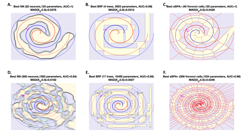
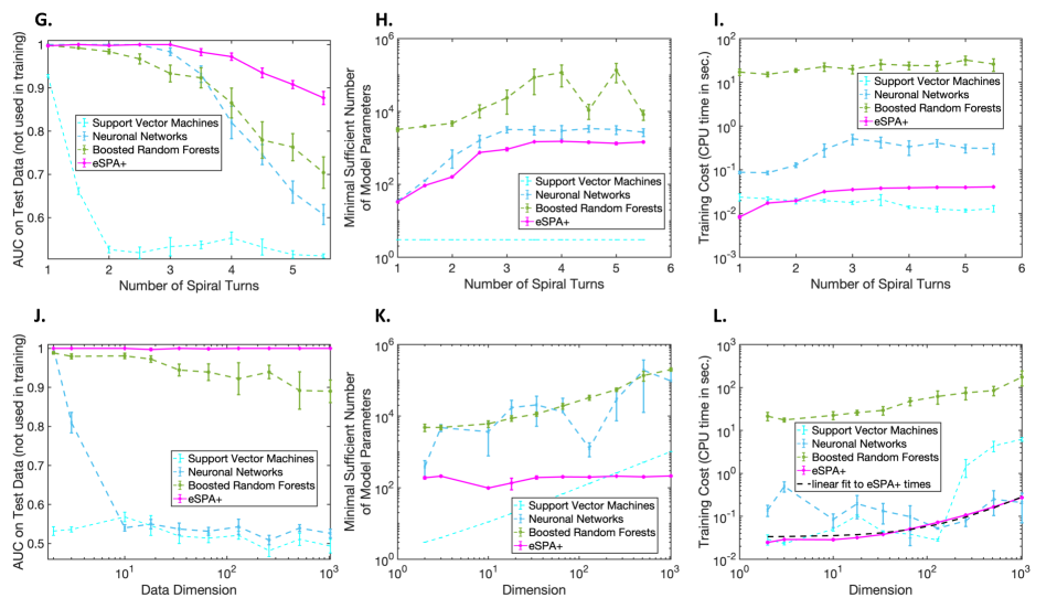
Figure 1: Swiss double-roll spiral and its extensions: MAP/MAD results for a common parameterization with $D=2$ and two full spiral turns (panels A-C), for an extension to four spiral turns (and all other benchmark parameters left the same as in [5], panels D-F). Panels G-I show comparisons for the changing number of example spirals, and panels J-L for the changing number of non-informative (uniformly-distributed) feature dimensions.

Synthetic examples: Swiss double-roll spiral and its extensions First, we will consider one of the most simple and standard AI classification benchmarks - a two-dimensional Swiss roll with two spirals, making two full turns (each spiral is characterized by a distinctive class affiliation, see Fig 1A-1C), the two spirals are intertwined in each other [5]. This is one of the most basics low-dimensional AI benchmarks, its advantage to the more complex synthetic problems is that it is very easily extendable to become more complex - and to cover more advanced scenarios. In contrast, more complex examples are much more difficult to be boiled down to the clear and insightful level of the Swiss double-roll in 2D. For example, Swiss double-roll is easily extendable to multiple dimensions: to illustrate applications of nonlinear dimensionality reduction approaches, one adds additional non-informative dimensions (usually with uniform data distribution) to the two dimensions in which the two spirals are distinguishable [14].

We start with the most common 2D benchmark parameter setting, that has two full turns for each of the spirals, and uses 512 random data points for training and another 512 for validation and testing (a $50\%-25\%-25\%$ cross-validation split) [5]. Panels A-C of Fig.1 show the results for this setting for the best performers among NNs (Fig. 1A), among boosted random forests (BRF, Fig. 1B), and for eSPA (Fig. 1C). Magenta circles denote the randomly selected point $X$ that has to be subject to an adversarial attack and MAD/MAP computation. Magenta crosses represent the computed endpoints $X^{*}$ of MAP for each of the methods. Panels D-F of Fig.1 illustrate the challenge of extending this simple benchmark with the increasing number of spiral turns - by keeping all other example parameters constant, including the size of the training data statistics that stays 512 as in the original benchmark from [5]. As can be seen from Fig. 1D-1F, with a growing number of spiral turns, increasing non-convexity of $\mathbb{P}_{L}(\cdot)$ (see contour-lines of Fig.1A-1F) results in the shorter adversarial pathways and smaller MADs. Panels Fig. 1G-1I show dependence of classifier performances for a changing number of spiral turns in the standard example, whereas panels Fig. 1J-1L illustrate how the performance of AI classifiers change with the added number of the non-informative uniformly distributed dimensions.

Biomedical examples: using MAP for a patient-specific computing of the minimal sufficient risk-mitigating therapeutic interventions Next, in Figs. 2 and 3 we see the results for the two biomedical applications: for the medical insurance claim database (Fig. 2) and for the deadly cardiac arrest data prediction problem based on patient data (Fig. 3). As the controllable/attackable features in the first example we consider the smoking status, the Body-Mass-Index (BMI) and the average number of steps the person is doing per day. In the second example (Fig. 3), we choose the amount of serum creatinine, the number of thrombocytes (platelets), the blood ejection fraction of the heart, the creatinine phosphokynase amount, the serum sodium amount and the smoking status as the attackable/controllable features. Links to these openly-accessible data sources are provided in the Section "Availability of data and material". As can be seen from the panels A-D of Figs. 2 and 3, eSPA is providing a superior prediction of cases on a test data (i.e., patient cases not used in training and validation) - it achieves the values AUC=0.98 for the first and AUC=0.90 for the second example. Computed MAPs (in panels E-H of Figs. 2-3) allow an interpretable - and mathematically-guaranteed minimal (due to the above Theorem 2) therapeutic intervention that would have allowed a reduction of risk with a certain predefined threshold $\delta$ (e.g., of the insurance claim risk with $\delta=0.9$ in Fig. 2 - or of deadly heart arrest risk with $\delta=0.5$ in Fig. 3). According to these results, approximately 48% of the insurance claiming individuals could have avoided claims only through an appropriate adjustment of BMI, of the number of daily steps and of their smoking status (see Fig. 2C). Approximately 23% of the patients (some of them very borderline, sadly) - who actually died of the heart attack - could have a possibility of reducing their death risk by at least 50% (see Fig. 3C). Moreover, obtained results very straightforwardly allow interpretable insights into the age-dependence of these optimal interventions (see Figs. 2F, 2H, 3F and 3H).

Conclusions Numerical questions behind the mathematical theory of adversarial attacks on AI systems are currently moving into the focus of AI research. Currently available numerical algorithms for adversarial attacks are based on gradient descent ideas - and are hampered by the issues of potentially slow convergence, non-convexity and ill-posednes of decision functions. This paper describes an alternative approach to adversarial attacks, establishing two theorems that give explicit analytically-solvable expressions for a minimal adversarial path in generalized linear models and locally uniquely-invertible classifiers - as well as providing straightforwardly-verifiable mathematical conditions and polynomially-scalable strongly-convex Quadratic Programming solvers for the optimal control and minimal adversarial path computation in entropic AI.

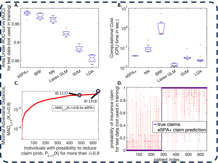
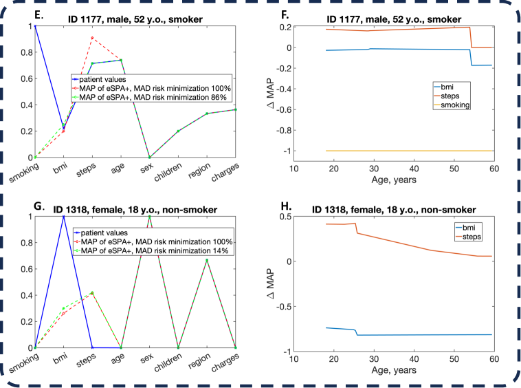
Figure 2: Computation of MAP and MAD for the insurance claim data from https://www.kaggle.com/datasets/easonlai/sample-insurance-claim-prediction-dataset. Explanations of the panels are in the paper text.

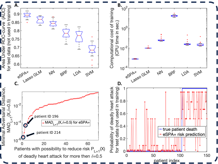
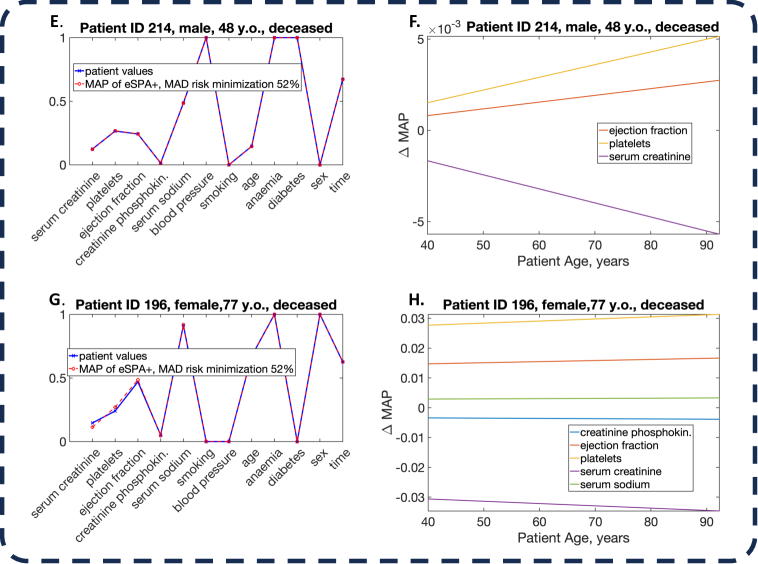
Figure 3: Computation of MAP and MAD for the predictions of death from the cardiac arrest data https://www.kaggle.com/datasets/andrewmvd/heart-failure-clinical-data. Explanations of the panels are in the paper text.

Availability of data, code and material The code implementing MAP and MAD computations introduced in the paper and reproducing the results from Fig. 1A-1F is provided at https://github.com/horenkoi/Minimal-Adversarial-Path-. Medical data used in Figs. 2 and 3 are available at https://www.kaggle.com/datasets/easonlai/sample-insurance-claim-prediction-dataset and https://www.kaggle.com/datasets/andrewmvd/heart-failure-clinical-data, respectively.

Acknowledgement The author thanks Rupert Klein (FU Berlin) for very motivating and helpful discussions.

References

- \bibcommenthead
- Bubeck et al. [2023] Bubeck, S., Chandrasekaran, V., Eldan, R., Gehrke, J., Horvitz, E., Kamar, E., Lee, P., Lee, Y.T., Li, Y., Lundberg, S., Nori, H., Palangi, H., Ribeiro, M.T., Zhang, Y.: Sparks of Artificial General Intelligence: Early experiments with GPT-4 (2023). https://www.microsoft.com/en-us/research/publication/sparks-of-artificial-general-intelligence-early-experiments-with-gpt-4/
- Xu et al. [2020] Xu, H., Ma, Y., Liu, H.-C., Deb, D., Liu, H., Tang, J.-L., Jain, A.K.: Adversarial attacks and defenses in images, graphs and text: A review. International Journal of Automation and Computing 17(2), 151–178 (2020) https://doi.org/10.1007/s11633-019-1211-x
- Wang et al. [2023] Wang, T.T., Gleave, A., Tseng, T., Pelrine, K., Belrose, N., Miller, J., Dennis, M.D., Duan, Y., Pogrebniak, V., Levine, S., Russell, S.: Adversarial policies beat superhuman go AIs. In: Krause, A., Brunskill, E., Cho, K., Engelhardt, B., Sabato, S., Scarlett, J. (eds.) Proceedings of the 40th International Conference on Machine Learning. Proceedings of Machine Learning Research, vol. 202, pp. 35655–35739. PMLR, ??? (2023). https://proceedings.mlr.press/v202/wang23g.html
- Chen et al. [2020] Chen, J., Jordan, M.I., Wainwright, M.J.: Hopskipjumpattack: A query-efficient decision-based attack. In: 2020 IEEE Symposium on Security and Privacy (SP), pp. 1277–1294 (2020). https://doi.org/10.1109/SP40000.2020.00045
- Haber and Ruthotto [2017] Haber, E., Ruthotto, L.: Stable architectures for deep neural networks. Inverse Problems 34(1), 014004 (2017) https://doi.org/10.1088/1361-6420/aa9a90
- Nocedal and Wright [2006] Nocedal, J., Wright, S.: Numerical Optimization. Springer, ??? (2006)
- He and Zheng [2020] He, L.J. JuncaiLi, Zheng, C.: Relu deep neural networks and linear finite elements. Journal of Computational Mathematics 38(3), 502–527 (2020) https://doi.org/10.4208/jcm.1901-m2018-0160
- Gerber et al. [2020] Gerber, S., Pospisil, L., Navandar, M., Horenko, I.: Low-cost scalable discretization, prediction, and feature selection for complex systems. Science Advances 6(5), 0961 (2020) https://doi.org/10.1126/sciadv.aaw0961
- Horenko [2020] Horenko, I.: On a scalable entropic breaching of the overfitting barrier for small data problems in machine learning. Neural Computation 32(8), 1563–1579 (2020) https://doi.org/10.1162/neco_a_01296
- Vecchi et al. [2022] Vecchi, E., Pospíšil, L., Albrecht, S., O’Kane, T.J., Horenko, I.: eSPA+: Scalable Entropy-Optimal Machine Learning Classification for Small Data Problems. Neural Computation 34(5), 1220–1255 (2022) https://doi.org/10.1162/neco_a_01490 https://direct.mit.edu/neco/article-pdf/34/5/1220/2008663/neco_a_01490.pdf
- Horenko [2022] Horenko, I.: Cheap robust learning of data anomalies with analytically solvable entropic outlier sparsification. Proceedings of the National Academy of Sciences 119(9), 2119659119 (2022) https://doi.org/10.1073/pnas.2119659119 https://www.pnas.org/doi/pdf/10.1073/pnas.2119659119
- Horenko et al. [2023] Horenko, I., Vecchi, E., Kardoš, J., Wächter, A., Schenk, O., O’Kane, T.J., Gagliardini, P., Gerber, S.: On cheap entropy-sparsified regression learning. Proceedings of the National Academy of Sciences 120(1), 2214972120 (2023) https://doi.org/10.1073/pnas.2214972120 https://www.pnas.org/doi/pdf/10.1073/pnas.2214972120
- Schrijver [1986] Schrijver, A.: Theory of Linear and Integer Programming. Wiley-Interscience, ??? (1986). https://www.bibsonomy.org/bibtex/2c05d22504b2f52da8a72d854b5043004/wvdaalst
- Bengio et al. [2003] Bengio, Y., Paiement, J.-F., Vincent, P., Delalleau, O., Roux, N.L., Ouimet, M.: Out-of-sample extensions for lle, isomap, mds, eigenmaps, and spectral clustering. In: Thrun, S., Saul, L.K., Schölkopf, B. (eds.) NIPS, pp. 177–184. MIT Press, ??? (2003). http://dblp.uni-trier.de/db/conf/nips/nips2003.html#BengioPVDRO03