Refer: An End-to-end Rationale Extraction Framework
for Explanation Regularization

Abstract

Human-annotated textual explanations are becoming increasingly important in Explainable Natural Language Processing. Rationale extraction aims to provide faithful (i.e., reflective of the behavior of the model) and plausible (i.e., convincing to humans) explanations by highlighting the inputs that had the largest impact on the prediction without compromising the performance of the task model. In recent works, the focus of training rationale extractors was primarily on optimizing for plausibility using human highlights, while the task model was trained on jointly optimizing for task predictive accuracy and faithfulness. We propose Refer, a framework that employs a differentiable rationale extractor that allows to back-propagate through the rationale extraction process. We analyze the impact of using human highlights during training by jointly training the task model and the rationale extractor. In our experiments, Refer yields significantly better results in terms of faithfulness, plausibility, and downstream task accuracy on both in-distribution and out-of-distribution data. On both e-SNLI and CoS-E, our best setting produces better results in terms of composite normalized relative gain than the previous baselines by 11% and 3%, respectively.

1 Introduction

Neural Language Models have emerged as State-of-The-Art (SoTA) performers in a wide range of Natural Language Processing (NLP) tasks Devlin et al. (2019); Liu et al. (2019). However, they are often perceived as opaque Rudin (2019); Doshi-Velez and Kim (2017); Lipton (2018), sparking significant interest in the development of algorithms that can automatically explain the behavior of these models Denil et al. (2015); Sundararajan et al. (2017); Camburu et al. (2018); Rajani et al. (2019); Luo et al. (2022).

In the field of self-explainable neural models, two prominent approaches have emerged: (i) Extractive Rationales (ERs, Zaidan et al., 2007; Bastings and Filippova, 2020), which involve selecting a subset of input features responsible for a prediction, and (ii) Natural Language Explanations (NLEs, Park et al., 2018; Hendricks et al., 2016; Kayser et al., 2021; Camburu et al., 2018), which generate human-readable justifications for predictions. The key aspects of interest for both ERs and NLEs are plausibility, which measures the alignment between model explanations and ground truth, and faithfulness, which measures how accurately the explanations reflect the decision-making process of the model. ERs offer concise explanations, serving as a means for users to assess the trustworthiness of a model. However, ERs may lack important reasoning details, such as feature relationships Wiegreffe et al. (2021). On the other hand, NLEs provide detailed justifications in natural language, complementing ERs by potentially offering more comprehensive explanations.

The evaluation of ERs involves assessing their plausibility and faithfulness. Plausibility refers to the extent to which a highlight explains a predicted label, as judged by human evaluators, or according to the similarity with gold highlights Yang et al. (2020); DeYoung et al. (2020). Faithfulness measures how accurately a highlight represents the decision process of the model – for example, by measuring to which extent the confidence in the predicted label changes after removing the highlighted words (comprehensiveness) or when only considering the highlighted words (sufficiency) Alvarez Melis and Jaakkola (2018); Wiegreffe and Pinter (2019).

Previous works largely focused on rationale extraction, which involves explaining the output of a model by identifying the input tokens that exert the greatest influence on model predictions Denil et al. (2015); Sundararajan et al. (2017); Jin et al. (2020); Lundberg and Lee (2017) and providing additional supervision signal Hase and Bansal (2022). The majority of prior works in this area have revolved around explanation regularization, a technique aimed at improving generalization in neural models by aligning machine rationales with human rationales Ross et al. (2017); Huang et al. (2021); Ghaeini et al. (2019); Kennedy et al. (2020); Rieger et al. (2020); Liu and Avci (2019). However, ERs are discrete distributions over the input text, which can be difficult to learn by neural models via back-propagation Niepert et al. (2021). In this work, we propose Refer, an End-to-end Rationale Extraction Framework for Explanation Regularization, which allows to back-propagate through the rationale extraction process. Specifically, Refer involves a differentiable rationale extractor, which selects the top-$k\%$ most important words from the textual input, which are then used by the model to generate a prediction.

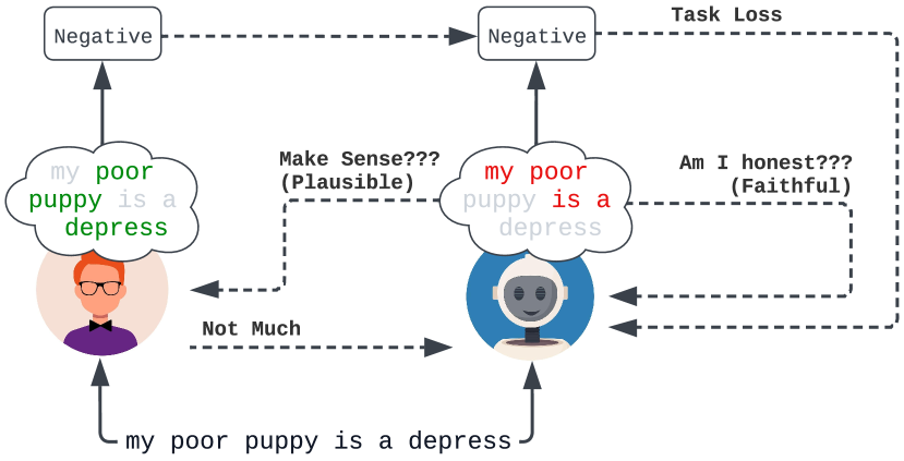
Figure 1: Explanation Regularization System: model is trained with human rationales while maintaining high task performance. In this case, the model predicts the correct label for incorrect reasons.

2 Related Works

The inherent complexity of neural models has given rise to concerns regarding their opacity Rudin (2019), particularly about the societal implications of employing neural models in high-stakes decision-making scenarios Bender et al. (2021). Therefore, explainability is of utmost importance for fostering trust, ensuring ethical practices, and maintaining the safety of NLP systems Doshi-Velez and Kim (2017); Lipton (2018).

Learning to Explain

Rationalization offers local explanations by providing a unique explanation for each prediction instead of a global explanation that covers the entire model Baehrens et al. (2010); Ribeiro et al. (2016). These explanations yield valuable insights for various purposes, including debugging, quantifying bias and fairness, understanding model behavior, and ensuring robustness and privacy Molnar (2022). However, obtaining direct supervision in the form of human-labeled rationales during training is not always feasible, which has led to the development of datasets that include human justifications for the true labels. These efforts enhance the interpretability of NLP models and address the limitations associated with direct supervision in learning to explain.

Post-hoc Explanations

Post-hoc explanations are another branch of interpretability research. These explanations often involve token-level importance scores. In the quest for effective post-hoc explanations, a balance must be struck between the clarity of semantics and the avoidance of counter-intuitive behaviors. Gradient-based explanations Sundararajan et al. (2017); Smilkov et al. (2017) provide clear semantics by describing the local impact of input perturbations on the outputs of the model. However, they can sometimes exhibit inconsistent behaviors Feng et al. (2018), and their effectiveness relies on the differentiability of the model. Alternatively, there are model-agnostic methods that do not rely on specific model properties. One notable example is Local Interpretable Model-agnostic Explanations (LIME, Ribeiro et al., 2016). These approaches approximate the behavior of the model locally by repeatedly making predictions on perturbed inputs and fitting a simple, explainable model over the resulting outputs.

Learning from Human Rationales

Recent research has focused on leveraging rationales to enhance the training of neural text classifiers. Zhang et al. (2016) introduced a rationale-augmented Convolutional Neural Network that explicitly identifies sentences supporting categorizations. Strout et al. (2019) demonstrated that incorporating rationales during training improves the quality of predicted rationales, as preferred by humans compared to models trained without explicit supervision Strout et al. (2019). In addition to integrated models, pipeline approaches have been proposed, where separate models are trained for rationale extraction and classification based on these extracted rationales Lehman et al. (2019); Chen et al. (2019). These approaches assume the availability of explicit training data for rationale extraction.

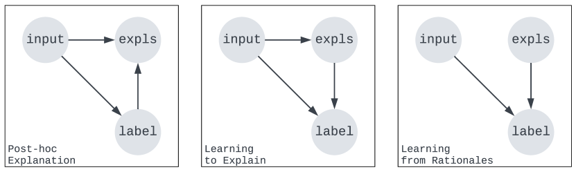
Figure 2: Computation graphs describing the relationships between post-hoc explanations, learning to explain, and learning from rationales.

Extractive Rationale Objectives

Several prior works have aimed to enhance the faithfulness of extractive rationales using Attribution Algorithms (AAs), which extract rationales via handcrafted functions Sundararajan et al. (2017); Ismail et al. (2021); Situ et al. (2021). However, AAs are not easily optimized and often require significant computational resources. Situ et al. (2021); Schwarzenberg et al. (2021) tackle the computational cost by training a model to mimic the behavior of an AA. Jain et al. (2020); Yu et al. (2021); Paranjape et al. (2020); Bastings and Filippova (2020); Yu et al. (2019); Lei et al. (2016) use Select-Predict Pipelines (SPPs) to generate faithful rationales. However, SPPs only guarantee sufficiency but not comprehensiveness DeYoung et al. (2020), and generally produce less accurate results, since they can only observe a portion of the input, and due to the challenges associated with gradient-based optimization and discrete distributions.

Regarding the plausibility of the rationales, existing approaches typically involve supervising neural rationale extractors Bhat et al. (2021) and SPPs Jain et al. (2020); Paranjape et al. (2020); DeYoung et al. (2020) using gold rationales. However, LM-based extractors lack training for faithfulness, and SPPs sacrifice task performance to achieve faithfulness by construction. Other works mainly focus on improving the plausibility of rationales Narang et al. (2020); Lakhotia et al. (2021); Camburu et al. (2018), often employing task-specific pipelines Rajani et al. (2019); Kumar and Talukdar (2020). In contrast, Refer jointly optimizes both the task model and rationale extractor for faithfulness, plausibility, and task performance and reaches a better trade-off w.r.t. these desiderata without suffering from heuristic-based approaches (e.g., AAs) disadvantages.

3 Model Architecture

Task Model

Consider $\mathcal{F}_{\text{task}}$ as the task model for text classification, where it consists of an encoder Vaswani et al. (2017) and a head. Let $\text{x}_{i}=[\text{x}^{t}_{i}]^{n}_{t=1}$ be $i^{th}$ input sequence with length $n$, and $\mathcal{F}_{\text{task}}(\text{x}_{i})\in\mathbb{R}^{M}$ be the logit vector for the output of the task model. We use $y_{i}=\arg\max_{j}[\mathcal{F}_{\text{task}}(\text{x}_{i})]_{j}$ to denote the class predicted by task model. Given that cross-entropy loss is used to train $\mathcal{F}_{\text{task}}$ to predict $y_{i}^{*}$, the task loss is defined as follow:

$$\mathcal{L}_{\text{task}}=\mathcal{L}_{\text{CE}}(\mathcal{F}_{\text{task}}(\text{x}_{i}),y_{i}^{*})$$ (1)

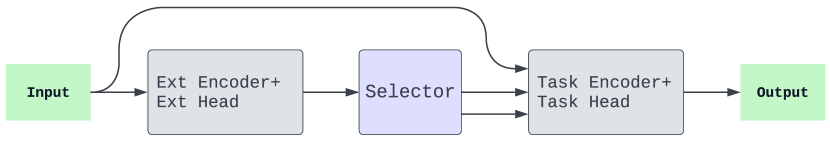
Figure 3: The pipeline for explanation regularization is a fully end-to-end approach where the task model’s output loss is back-propagated through all components, resulting in a compromised performance that considers all training criteria.

Rationale Extractor

Let $\mathcal{F}_{\text{ext}}$ denote a rationale extractor, such that $\text{s}_{i}=\mathcal{F}_{\text{ext}}(\text{x}_{i})$. Given $\mathcal{F}_{\text{task}}$, $\text{x}_{i}$, and $y_{i}$, the goal of rationale extraction is to output vector $\text{s}_{i}=[s^{t}_{i}]^{n}_{t=1}\in\mathbb{R}^{n}$, such that each $s^{t}_{i}$ is an importance score indicating how strongly token $\text{x}^{t}_{i}$ influenced $\mathcal{F}_{\text{task}}$ to predict class $y_{i}$. The final rationales are typically obtained by binarizing $\text{s}_{i}$ as $\text{r}_{i}^{(k)}\in\{0,1\}^{n}$, via the top-$k\%$ strategy DeYoung et al. (2020); Jain et al. (2020); Pruthi et al. (2022); Chan et al. (2021).

To capture the degree to which the snippets within the extracted rationales are sufficient for a model to make a prediction, we measure the disparity in model confidence when considering the complete input versus only the extracted rationales. A small difference suggests the high importance of extracted rationales.

$$\mathcal{L}_{\text{suff-diff}}=\mathcal{L}_{\text{CE}}(\mathcal{F}_{\text{task}}(\text{r}_{i}^{(k)}),y_{i}^{*})$$ (2)

$$-\mathcal{L}_{\text{CE}}(\mathcal{F}_{\text{task}}(\text{x}_{i}),y_{i}^{*})$$

Following Chan et al. (2022), to avoid negative losses, we can use margin $m_{s}$ to impose a lower bound on $\mathcal{L}_{\text{suff-diff}}$, yielding the following margin criterion:

$$\mathcal{L}_{\text{suff}}=\max(-m_{s},\mathcal{L}_{\text{suff-diff}})+m_{s}$$ (3)

To compute comprehensiveness we create contrast examples for $\text{x}_{i}$, $\tilde{\text{x}}_{i}=\text{x}_{i}\backslash\text{r}_{i}^{(k)}$, which is $\text{x}_{i}$ with the predicted rationales $\text{r}_{i}$ removed Zaidan et al. (2007). Similar to Equation 2, we measure the difference in model confidence between considering the complete input and the contrast set $\tilde{\text{x}}_{i}$. A high score here implies that the rationales were influential in the prediction.

$$\mathcal{L}_{\text{comp-diff}}=\mathcal{L}_{\text{CE}}(\mathcal{F}_{\text{task}}(\text{x}_{i}),y_{i}^{*})$$ (4)

$$-\mathcal{L}_{\text{CE}}(\mathcal{F}_{\text{task}}(\tilde{\text{x}}_{i}),y_{i}^{*})$$

Repeatedly, we enforce $\mathcal{L}_{\text{comp-diff}}$ to be positive as follows:

$$\mathcal{L}_{\text{comp}}=\max(-m_{c},\mathcal{L}_{\text{comp-diff}})+m_{c}$$ (5)

Finally, the selection of the tokens for matching the human highlights can be cast as a binary classification problem, and the plausibility loss is computed using the binary cross-entropy (BCE) loss function:

$$\mathcal{L}_{\text{plaus}}=-\sum_{t}\text{r}_{i}^{*,t}\log(\mathcal{F}_{\text{ext}}(\text{x}_{i}^{t}))$$ (6)

where $\text{r}_{i}^{*}$ is the gold rationale for input $\text{x}_{i}$ of length $t$. This leads to the following multi-task learning objective:

$$\mathcal{L} =\mathcal{L}_{\text{task}}+\alpha_{\text{f}}\mathcal{L}_{\text{faith}}+\alpha_{\text{p}}\mathcal{L}_{\text{plaus}}$$

$$=\mathcal{L}_{\text{task}}+\alpha_{\text{c}}\mathcal{L}_{\text{comp, K}}+\alpha_{\text{s}}\mathcal{L}_{\text{suff, K}}+\alpha_{\text{p}}\mathcal{L}_{\text{plaus}}$$

Back-Propagating Through Rationale Extraction

To back-propagate through the rationale extraction process, we use Adaptive Implicit Maximum Likelihood Estimation (AIMLE, Minervini et al., 2023), a recently proposed low-variance and low-bias gradient estimation method for discrete distribution that does not require significant hyper-parameter tuning. AIMLE is an extension of Implicit Maximum Likelihood Estimation (IMLE, Niepert et al., 2021), a perturbation-based gradient estimator where the gradient of the loss w.r.t. the token scores $\nabla_{\mathbf{s}}\mathcal{L}$ is estimated as $\nabla_{\mathbf{s}}\mathcal{L}\approx\mathbf{r}(\mathbf{s}+\epsilon)-\mathbf{r}(\mathbf{s}+\lambda\nabla_{\mathbf{r}}\mathcal{L}+\epsilon)$, where $\epsilon$ denotes Gumbel noise, $\mathbf{r}$ denotes the top-$k$% function, and $\lambda$ is a hyper-parameter selected by the user. AIMLE removes the need for the user to select $\lambda$ by automatically identifying the optimal $\lambda$ for a given learning task.

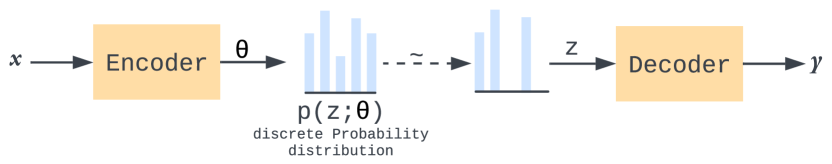
Figure 4: Illustration of the learning problem. $z$ is the discrete latent structure, $x$ and $y$ are feature inputs and target outputs, Encoder maps $\mathcal{X}\mapsto\theta$, Decoder maps $\mathcal{Z}\mapsto\mathcal{Y}$, and $p(z;\theta)$ represents the discrete probability distribution. The dashed path indicates non-differentiability.

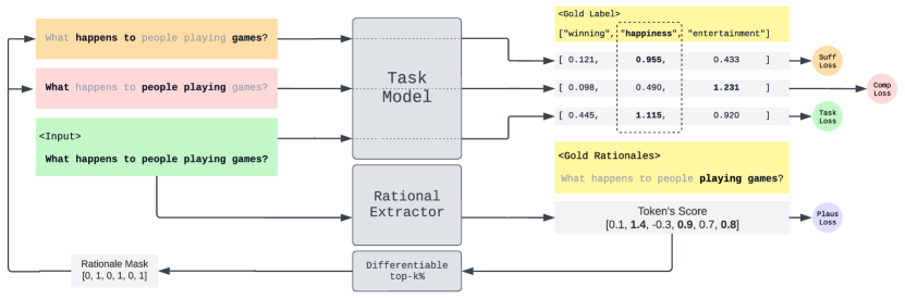
Figure 5: Refer Pipeline. The Task Model is trained using (i) Task Loss, (ii) Sufficiency Loss, and (iii) Comprehensiveness Loss, while the Rationale Extractor is trained through backpropagation using (i) Plausibility Loss, (ii) Sufficiency Loss, and (iii) Comprehensiveness Loss. This approach ensures a high level of consistency across each criterion, as all components are aware of each other’s status and can adapt to strike a balance among the three criteria.

4 Research Questions

RQ1: Does training the model on human highlights improve the generalization properties of the model?

Nowadays, machine learning systems can learn to capture spurious correlations in the data for solving any given task, and often struggle in more challenging cases McCoy et al. (2019). When models are allowed to make predictions without considering rationales-related criteria—faithfulness and plausibility—the rationales extracted by the model can be incomprehensible and lack meaningful interpretations Vig and Belinkov (2019). Without understanding the factors and information that influence the predictions of the model, it becomes difficult to trust or explain its outputs. In certain contexts, faithful explanations are crucial – for example, they can be used to determine whether a model relies on protected attributes, such as gender or religious group Pruthi et al. (2020). McCoy et al. (2019) propose the hypothesis that neural natural language inference (NLI) models might rely on three fallible syntactic heuristics: (i) lexical overlap, (ii) subsequences, and (iii) constituents. To evaluate whether the models have indeed adopted these heuristics, we use Heuristic Analysis for NLI Systems (HANS, McCoy et al., 2019), which includes a variety of examples where such heuristics fail, providing a means to assess a model’s reliance on these heuristics. Table 7 shows instances of these heuristics in the HANS dataset.

Faithfulness refers to the degree to which an explanation provided by a model accurately reflects the information utilized by the model to make a decision (Jacovi and Goldberg, 2020). they can be used to determine whether a model is relying on protected attributes, such as gender or religious group Pruthi et al. (2020).

RQ2: How can we make machines imitate human rationales?

Human rationales are often derived from their extensive background knowledge and understanding of various concepts. While language models (LMs) possess some degree of this knowledge, they face challenges in balancing between optimizing for task performance and meeting the criteria for extractive explanations. Therefore, balancing plausibility, faithfulness, and task accuracy presents a challenging task. A model can reflect its inner process to make a prediction (faithful), but it may not make sense for humans (implausible). On the other hand, a model that returns convincing rationales (plausible) without using them during decision-making is not very useful (unfaithful).

RQ3: Does training the model on a small number of human highlights improve its generalization properties?

Humans can efficiently learn new tasks with only a few examples by leveraging their prior knowledge. Recent approaches for rationalizing rely on a large number of labeled training examples, including task labels and annotated rationales for each instance. Obtaining such extensive annotations is often infeasible for many tasks. Additionally, fine-tuning LMs, which typically have billions of parameters, can be expensive and prone to overfitting. Given the high cost of human annotations, a more practical approach involves incorporating a limited amount of human supervision. We investigate the characteristics of effective rationales and demonstrate that making the neural model aware of its rationalized predictions can significantly enhance its performance, especially in low-resource scenarios.

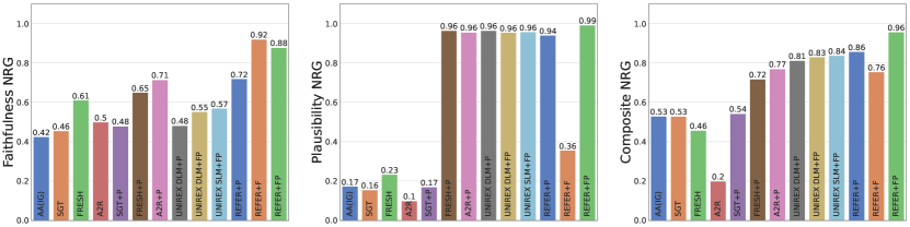
Figure 6: Comparison of models w.r.t. faithfulness NRG (FNRG), plausibility NRG (PNRG), and composite NRG (CNRG). +P, +F, +FP indicate whether the model was regularized for plausibility, faithfulness, or both.

RQ4: Do the learned rationale extractors generalize to OOD data?

The poor performance of models on OOD datasets can stem from limitations in the model’s architecture, insufficient signals in the OOD training set, or a combination of both McCoy et al. (2019). An NLI system that correctly labels an example may not do so by understanding the meaning of the sentences but rather by relying on the assumption that any hypothesis with words appearing in the premise is entailed by the premise Dasgupta et al. (2018); Naik et al. (2018). Gururangan et al. (2018) raises doubts about whether models trained on the SNLI dataset truly learn language comprehension or primarily rely on spurious correlations, also known as artifacts. For instance, words like "friends" and "old" frequently appear in neutral hypotheses. To analyze this, we evaluate our model on contrast sets Gardner et al. (2020) as well as unseen data, which are (mostly) label-changing small perturbations on instances to understand the true local boundary of the dataset. Essentially, they help us understand if the rationale extractor has learned any dataset-specific shortcuts. Table 9 shows samples for both label-changing and and non-label-changing instances modified by Li et al. (2020).

5 Experiment

5.1 Baselines

The first class of baselines is AAs, which do not involve training $\mathcal{F}_{\text{ext}}$ and is applied post hoc (i.e., they do not impact $\mathcal{F}_{\text{task}}$’s training). Integrated Gradient baseline (AA (IG), Sundararajan et al., 2017) is utilized as a baseline for this class. Saliency Guided Training (SGT, Ismail et al., 2021) is another baseline that uses a sufficiency-based criterion to regularize $\mathcal{F}_{\text{task}}$, such that the AA yields faithful rationales for $\mathcal{F}_{\text{task}}$.

Another approach is the Select-Predict Pipeline (SPP), wherein $\mathcal{F}_{\text{task}}$ is trained to solve a given task using only the tokens chosen by $\mathcal{F}_{\text{ext}}$ Jain et al. (2020); Yu et al. (2019); Paranjape et al. (2020); therefore, SPPs aim for "faithfulness by construction". FRESH Jain et al. (2020) and A2R Yu et al. (2019) have been proposed to produce faithful rationales: FRESH relies on training $\mathcal{F}_{\text{task}}$ and $\mathcal{F}_{\text{ext}}$ separately, while A2R aims to improve $\mathcal{F}_{\text{task}}$’s task performance by regularizing it with an attention-based predictor that utilizes the full input Jain et al. (2020); Yu et al. (2019).

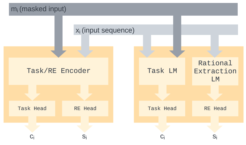
Figure 10: Shared LM (left) and Dual LM (right) architecture. Using shared LM, the task model and rational extractor share the same encoder. While in the Dual LM model, they are completely separate

The most recent pipeline is UNIREX Chan et al. (2022), which considers two main architecture variants: (i) Dual LM (DLM), where $\mathcal{F}_{\text{task}}$ and $\mathcal{F}_{\text{ext}}$ are two separate Transformer-based LMs with the same encoder architecture (ii) Shared LM (SLM), where $\mathcal{F}_{\text{task}}$ and $\mathcal{F}_{\text{ext}}$ share encoder, while $\mathcal{F}_{\text{ext}}$ has its own output head. Figure 10 shows the architecture for DLM and SLM in UNIREX. DLM provides more capacity for $\mathcal{F}_{\text{ext}}$, which can help $\mathcal{F}_{\text{ext}}$ provide plausible rationales. While SLM leverages multitask learning and improve faithfulness since $\mathcal{F}_{\text{ext}}$ has greater access to information about $\mathcal{F}_{\text{task}}$’s reasoning process Chan et al. (2022). Refer benefits from both SLM and DLM architectures by establishing communication between separate $\mathcal{F}_{\text{task}}$ and $\mathcal{F}_{\text{ext}}$ using back-propagation.

5.2 Metrics

To evaluate faithfulness, plausibility, and task performance, we adopt the metrics established in the ERASER benchmark DeYoung et al. (2020) and UNIREX Chan et al. (2022). For assessing faithfulness, we use comprehensiveness and sufficiency, and calculate the final comprehensiveness and sufficiency metrics using the area-over-precision curve (AOPC). Measuring exact matches between predicted and reference rationales is likely too strict; thus, DeYoung et al. (2020) also consider the Intersection-Over-Union (IOU) which permits credit assignment for partial matches. We use these partial matches to calculate the Area Under the Precision-Recall Curve (AUPRC) and Token F1 (TF1) to quantify the similarity between the extracted rationales and the gold rationales DeYoung et al. (2020); Narang et al. (2020). Also, we use accuracy and macro F1 to evaluate the task model performance on CoS-E and e-SNLI, respectively. To compare different methods w.r.t. all three desiderata, Chan et al. (2022) utilized the Normalized Relative Gain (NRG) metric that maps all raw scores to range $[0,1]$ — the higher the better. Finally, to summarize all of the raw metrics, we compute single NRG score by averaging the NRG scores for faithfulness, plausibility, and task accuracy.

5.3 Datasets

We primarily experiment with the CoS-E Rajani et al. (2019) and e-SNLI Camburu et al. (2018) datasets, all of which have gold rationale annotations from ERASER DeYoung et al. (2020). For the OOD generalization evaluation, we consider MNLI Williams et al. (2018) and HANS McCoy et al. (2019).

CoS-E

Rajani et al. (2019) consists of multiple-choice questions and answers taken from the work of Talmor et al. (2019). It includes supporting rationales for each question-answer pair in two forms. Extracted supporting snippets and free-text descriptions that provide a more detailed explanation of the reasoning behind the answer choice.

e-SNLI

Camburu et al. (2018) is an augmentation of the SNLI corpus Bowman et al. (2015) and includes human rationales as well as natural language explanations. For neutral pairs, annotators could only highlight words in the hypothesis. Furthermore, they consider explanations involving contradiction or neutrality to be correct as long as at least one piece of evidence in the input is highlighted. Focusing on the hypothesis and allowing partial highlighting of evidence leads to the collection of non-comprehensive highlights in the dataset.

MNLI

Williams et al. (2018) covers a broader range of written and spoken text, subjects, styles, and levels of formality compared to SNLI. It was introduced to determine the logical relationship between two given sentences. To evaluate the plausibility metrics on OOD data, we performed a random sampling of 50 instances from the MNLI validation split and annotated them manually w.r.t. gold labels. We referred to this particular subset of data as e-MNLI. Table 6 shows instances from e-MNLI for different labels. To conduct additional OOD generalization evaluation, we utilized two OOD Contrast Sets called MNLI-Contrast and MNLI-Original. These contrast sets were created by slightly modifying the original MNLI instances Li et al. (2020). In MNLI-Contrast, the modification changes the original label, while in MNLI-Original, the original label remains the same. Examples of these contrast sets are shown in Table 9.

HANS

McCoy et al. (2019) is designed to evaluate the capability of NLI systems to rely on heuristics and patterns instead of genuine understanding. HANS consists of sentence pairs carefully crafted to mislead models using three heuristic categories: Lexical Overlap, Subsequence, and Constituent. Instances for each heuristic are given in Table 7. By evaluating models on the HANS dataset, researchers can gain insights into the limitations and robustness of NLI systems.

6 Results

RQ1: Does training the model on human highlights improve the generalization properties of the model?

We label with +P and +FP the models trained by optimizing for plausibility and jointly faithfulness and plausibility, respectively. Figure 6 displays the main results for e-SNLI in terms of NRG. Overall, REFER+FP achieved the highest composite NRG, improving over the strongest baseline (UNIREX SLM+FP) by 12%. Regarding plausibility, models explicitly trained for plausibility (+P) or both faithfulness and plausibility (+FP) achieved similar results, with REFER+FP outperforming the second-best model by 3%. Regarding faithfulness, Refer achieved the highest score in all three configurations. An interesting finding is that even when training Refer and A2R solely for plausibility (REFER+P and A2R+P), their faithfulness NRG scores remain considerably higher than all other methods. Detailed results are shown in Table 10 and Table 11. Additionally, we analyzed the model’s predictions on correctly labeled instances compared to falsely labeled ones, as presented in Table 1. Surprisingly, although the model achieves relatively high plausibility scores, the sufficiency and comprehensiveness metrics are low when the model predicts the wrong label. This suggests that even when human rationales are extracted from the inputs, the model does not strongly rely on them in falsely labeled input.

The extracted rationales by the model, shown in Table 2, demonstrate the impact of regularization on explanation regularization. Without ER regularization, the model’s reasoning tends to rely on specific data patterns and heuristics rather than meaningful explanations. In contrast, when the model is regularized on ER, the quality of the rationales improves significantly in terms of faithfulness and plausibility. For instance, the example highlights the selection of "man pushing cart" and "woman smoking cigarette" as rationales to predict the label contradiction. The evaluation metrics for faithfulness on e-SNLI in Table 4 further support the notion that the model genuinely relies on these rationales for its predictions.

Table 1: Comparison of ER metrics for truly predicted labels and falsely predicted labels. (↑) indicates the higher value is better and (↓) the lower is better.

Metrics	True Predictions	Wrong Predictions
Sufficiency AOPC (↓)	0.0488	0.1566
Comprehensiveness AOPC (↑)	0.3311	0.3057
Plausibility TF1 (↑)	0.8016	0.7012
Plausibility AUPRC (↑)	0.8834	0.7350

Table 2: Refer highlights on e-SNLI. Instead of visualizing hard tokens selected by the model, we highlighted all the words w.r.t. their score.

Model	Highlights
Original Instance	Premise: A man in green pants and blue shirt pushing a cart. Hypothesis: A woman is smoking a cigarette. Label: contradiction
Refer without ER regularization	Premise: A man in green pants and blue shirt pushing a cart . Hypothesis: A woman is smoking a cigarette . Predict: contradiction
Refer with ER regularization	Premise: A man in green pants and blue shirt pushing a cart . Hypothesis: A woman is smoking a cigarette . Predict: contradiction

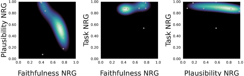
Figure 7: Results distribution of CoS-E dev split for different faithfulness and plausibility weights and $k$=50%. Kernel Density Estimation is used to have smoothed distribution over discrete data points for visualization purposes.

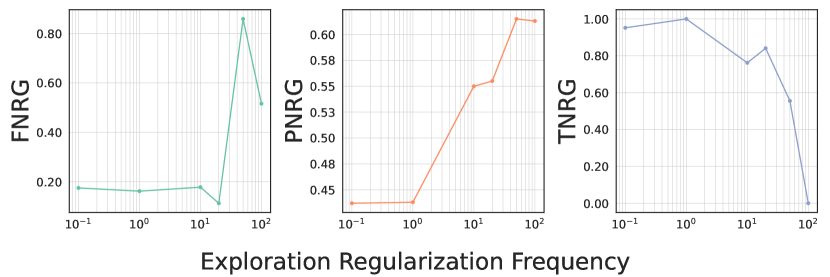
Figure 8: Comaprioson of different models w.r.t. faithfulness NRG (FNRG), plausibility NRG (PNRG), and composite NRG (CNRG).

RQ2: How can we make machines imitate humans’ rationales?

Figure 7 shows the distribution of the results for different combinations of faithfulness and plausibility loss weights on the CoS-E validation set. We trained the model for $(\alpha_{f},\alpha_{p})\in\{0.0,0.5,1.0\}^{2}$. Based on the results, there is a slight reverse correlation between plausibility and faithfulness. However, the task shows relatively stable behavior over faithfulness and plausibility variation. This means that, with our pipeline, we cannot reach a higher plausibility and faithfulness trade-off from a certain level on CoS-E.

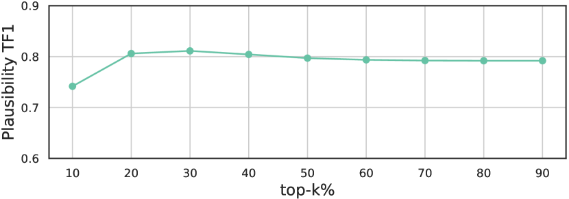
Figure 9: Plausiblity TF1 score of model trained for top-$50$% and evaluated for other top-$k$%s.

RQ3: How would small supervision of human highlight help?

We conducted experiments to investigate how our model behaves when different percentages of human-annotated data are included in the training set. Figure 8 showcases the outcomes obtained for all training criteria when varying percentages of human annotation were used: 0.1%, 1%, 10%, 20%, 50%, and 100%. The results indicate that until 10% of the data is annotated by humans, the plausibility remains consistent. On the other hand, Refer achieves comparable plausibility to 100% human supervision with just 50% of human annotation. This means Refer enables effective plausibility optimizations using minimal gold rationale supervision. In contrast, task performance is reduced by increasing the human rationale supervision since the model should learn from human highlights instead of repetitive patterns. Faithfulness does not exhibit a clear relationship with the availability of gold rationales, as it relies on the model’s intrinsic features rather than human-provided rationales.

Table 3: Comparison of the performance of Refer without explanation regularization on ID and OOD dataset.

Metrics	ID without ER regularization		OOD Datasets				Contrast Test
	e-SNLI		MNLI	HANS	e-MNLI		MNLI-Contrast	MNLI-Original
Task Accuracy (↑)	90.47		74.65	67.09	76.00		82.66	88.72
Task Macro F1 (↑)	90.48		74.80	28.57	75.93		60.25	88.74
Sufficiency AOPC (↓)	0.205		0.206	0.305	0.249		0.226	0.201
Comprehensiveness AOPC (↑)	0.243		0.212	0.272	0.224		0.210	0.249
Plausibility TF1 (↑)	0.254		N/A	N/A	0.197		N/A	N/A
Plausibility AUPRC (↑)	0.211		N/A	N/A	0.167		N/A	N/A

Table 4: Comparison of the performance of Refer with explanation regularization on ID and OOD dataset.

Metrics	ID with ER regularization		OOD Datasets				Contrast Test
	e-SNLI		MNLI	HANS	e-MNLI		MNLI-Contrast	MNLI-Original
Task Accuracy (↑)	90.33		74.10	66.06	78.00		82.11	88.37
Task Macro F1 (↑)	90.36		74.13	27.75	78.11		59.92	88.44
Sufficiency AOPC (↓)	0.059		0.109	0.071	0.100		0.091	0.050
Comprehensiveness AOPC (↑)	0.329		0.310	0.320	0.315		0.321	0.329
Plausibility TF1 (↑)	0.792		N/A	N/A	0.616		N/A	N/A
Plausibility AUPRC (↑)	0.869		N/A	N/A	0.445		N/A	N/A

RQ4: Does learned rationale extractor generalize over OOD data?

Table 3 and Table 4 show the Refer results on ID and OOD datasets. In both Tables Refer is trained on ID dataset and evaluated over ID and OOD sets. We consider the results from Table 3 as the baseline and analyze the effect of ER regularization in Table 4. When we train the model with explanation regularization, faithfulness and sufficiency are enhanced. On MNLI, sufficiency improves from 0.206 to 0.109, while on HANS, it goes from 0.249 to 0.071. Regarding Comprehensiveness, training the model along with ER regularization improves the baseline from 0.212 to 0.310 on MNLI and from 0.272 to 0.320 on HANS. Besides, results on e-MNLI in Table 4 show that the plausibility of OOD is significant and comparable to the ID data. Similarly, the comprehensiveness and sufficiency improve on both MNLI-Contrast and MNLI-Original. However, the results on MNLI-Original seem to be better, especially w.r.t task macro F1, which means the model performs equally well predicting different labels.

Another interesting finding is that the model trained for a specific top-$k$% performs well on other top-$k$% during inference w.r.t. plausibility. Figure 9 display roughly stable behavior of the model trained for top-50% and evaluated for other top-$k$% w.r.t. plausibility TF1. This means the model tends to select rationales among human highlights even with a low number of $k$. Table 8 illustrates the rationale selected by the model trained for top-50% and evaluated for different $k$s.

7 Conclusions

In this paper, we propose Refer, a rationale extraction framework that jointly trains the task model and the rationale extractor to optimize downstream task performance, faithfulness, and plausibility. Being fully end-to-end, thanks to Adaptive Implicit Maximum Likelihood Estimation (Minervini et al., 2023), enables the task model and the rationale extractor to be jointly optimized for these criteria, therefore aware of each other behavior and adopting their parameter to improve their performance and obtain a better balance. We then analyze several aspects of the rationale extraction process, investigating how human rationales affect the model behavior; how the model can imitate human-generated rationales; and to what extent the learned models can generalize on OOD datasets. Finally, by answering all these questions, we compare Refer performance with other methods and architectures and illustrate that our model outperforms previous models in most cases.

Acknowledgments

Reza was funded by the Thesis Abroad Scholarship from the Department of Computer Science and Engineering (DISI) at the University of Bologna. Pasquale was partially funded by the European Union’s Horizon 2020 research and innovation program under grant agreement no. 875160, ELIAI (The Edinburgh Laboratory for Integrated Artificial Intelligence) EPSRC (grant no. EP/W002876/1), an industry grant from Cisco, and a donation from Accenture LLP, and is grateful to NVIDIA for the GPU donations. This work was supported by the Edinburgh International Data Facility (EIDF) and the Data-Driven Innovation Programme at the University of Edinburgh.

Appendix A Model Detail

Transformers-based models, such as BERT, have been one of the most successful deep learning models for NLP. Unfortunately, one of their core limitations is the quadratic dependency (mainly in terms of memory) on the sequence length due to their full attention mechanism. To remedy this, Zaheer et al. (2020) proposed BigBird, a sparse attention mechanism that reduces this quadratic dependency to linear. They show that BigBird is a universal approximator of sequence functions and is Turing complete, thereby preserving these properties of the quadratic, full attention model. Along the way, their theoretical analysis reveals some of the benefits of having O(1) global tokens (such as CLS) that attend to the entire sequence as part of the sparse attention mechanism. The proposed sparse attention can handle sequences of length up to eight times what was previously possible using similar hardware. Due to the capability to handle longer contexts, BigBird drastically improves performance on various NLP tasks such as question answering and summarization.

Appendix B Hyperparameters

In our implementation, we utilize BigBird-Base Zaheer et al. (2020) as the backbone for both $\mathcal{F}_{\text{task}}$ and $\mathcal{F}_{\text{ext}}$. This choice enables us to effectively handle input sequences of considerable length, accommodating up to 4096 tokens. We used AIMLE, which uses adaptive target distribution with alpha and beta initialized to 1 and 0, respectively. Throughout all experiments, we maintain a consistent learning rate of $2\times 10^{-5}$ and employ an effective batch size of 32. Our training process spans a maximum of 10 epochs, with early stopping applied after 5 epochs of no significant improvement. To ensure optimal performance, we focus our hyperparameter tuning efforts on the weights associated with faithfulness and plausibility losses, specifically $\alpha_{\text{c}}=\alpha_{s}=\alpha_{\text{f}}$, and $\alpha_{\text{p}}$ as well as top-$k\%$. We applied a grid search across various configurations and evaluated their impact on comprehensiveness, sufficiency, plausibility scores, and task performance. The entire implementation is carried out using the PyTorch-Lightning framework Paszke et al. (2019); Falcon (2019), which provides a streamlined and user-friendly environment for deep learning experiments.

Table 5: Examples of highlights differing in comprehensiveness and sufficiency

Instance with Highlight	Type of Highlight
Premise: People are stretching on yoga mats. Hypothesis: They stretched on bikes. Label: contradiction	Premise:People are stretching on yoga mats. Hypothesis:They stretched on bikes. (sufficient)
Premise: People on bicycles waiting at an intersection. Hypothesis: There are people on bicycles. Label: entailment	Premise: People on bicycles waiting at an intersection. Hypothesis:There are people on bicycles. (comprehensive)
Premise: People on bicycles waiting at an intersection. Hypothesis: Some people on bikes are stopped at a junction. Label: neutral	Premise: People on bicycles waiting at an intersection. Hypothesis: Some people on bikes are stopped at a junction. (¬ sufficient)

Appendix C OOD Generalization

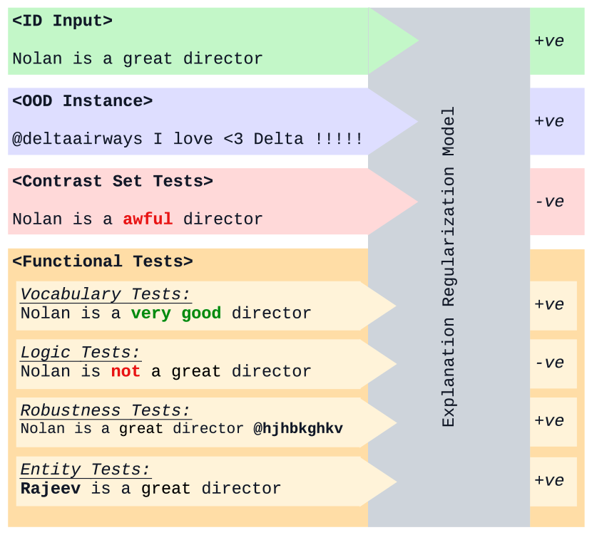
Figure 11: ER-TEST Framework - Apart from existing ID evaluations of ER criteria, ER-TEST evaluates ER’s impact on OOD generalization along three dimensions: A. Unseen datasets, B. Contrast set tests, and C. Functional tests.

Table 6: e-MNLI instances for different labels. Following e-SNLI for neutral labels only tokens in hypothesis are highlighted.

Instances with Highlights	Label
Premise: They drive it around the country in a dilapidated ice-cream truck trying to keep it cool. Hypothesis: They used an ice cream truck to try and keep it from getting warm.	entailment
Premise: Then he turned to Tommy. Hypothesis: He talked to Tommy.	neutral
Premise: but i’ve lived up here all my life and i’m fifty eight years old so i i could Hypothesis: I have moved somewhere else in my life.	contradiction

Out-of-distribution (OOD) generalization refers to the ability of a model to accurately handle data samples that deviate from the distribution of its training data. OOD generalization is a critical challenge in NLP tasks and plays a pivotal role in ensuring the reliability and effectiveness of NLP models in real-world applications. Effective OOD generalization in NLP requires models to capture and understand the underlying linguistic properties and generalizable patterns rather than relying on memorization or overfitting specific training instances. However, despite the growing interest in OOD generalization, existing evaluations in the field of explanation robustness have been limited in scope and coverage. Existing works primarily evaluate explanation regularization models via in-distribution (ID) generalization Zaidan et al. (2007); Lin et al. (2020); Huang et al. (2021), though a small number of works have done auxiliary evaluations of OOD generalization Ross et al. (2017); Kennedy et al. (2020); Rieger et al. (2020). Consequently, there is a lack of comprehensive understanding regarding the impact of explanation robustness on OOD generalization. To address this gap, Joshi et al. (2022) introduce ER-TEST, a unified benchmark specifically designed to assess the OOD generalization capabilities of explanation regularization models across three dimensions. These dimensions include evaluating models on (i) unseen datasets, (ii) conducting contrast set tests to measure their ability to handle diverse and challenging inputs, and (iii) functional tests which include four scopes: vocabulary tests, logic tests, robustness tests, and entity tests – the functional test is not included in our work. We leave this field for future work – to assess their reasoning and inference capabilities. Examples of each dimension are shown in Figure 11.

Ideally, we would like the explanation regularization model to perform well on all three aspects during the evaluation of OOD data. However, since the datasets for OOD evaluation do not contain human-annotated rationales there is no possibility of assessing the plausibility criteria. By addressing the OOD generalization challenge, NLP models can achieve greater robustness, adaptability, and practical utility in real-world scenarios, thus advancing the field of natural language processing and can better handle challenging scenarios.

Table 7: The heuristics targeted by the HANS dataset, along with examples of incorrect entailment predictions that these heuristics would lead to.

Heuristic	Definition	Example
Lexical overlap	The premise entails all hypotheses constructed from its own words.	The judges admired the doctors. $\xrightarrow{\text{Wrong}}$ The doctors admired the judges .
Subsequence	The premise entails all of its contiguous subsequences.	The lawyers believed the bankers resigned. $\xrightarrow{\text{Wrong}}$ The lawyers believed the bankers.
Constituent	The premise entails all complete subtrees in its parse tree.	Probably the tourists waited. $\xrightarrow{\text{Wrong}}$ The tourists waited.

Table 8: Comparison of rationales extracted by Refer trained on $k$=50%. We forced the model for other $k$ to see how it selects rationales.

Dataset	Test Instance
Gold	Premise: a woman wearing a pink tank top holding a mug of liquid Hypothesis: A woman in a blue tank top holding a car. Label: contradiction
k=20%	Premise: a woman wearing a pink tank top holding a mug of liquid Hypothesis: A woman in a blue tank top holding a car.
k=30%	Premise: a woman wearing a pink tank top holding a mug of liquid Hypothesis: A woman in a blue tank top holding a car.
k=40%	Premise: a woman wearing a pink tank top holding a mug of liquid Hypothesis:A woman in a blue tank top holding a car.
k=50%	Premise: a woman wearing a pink tank top holding a mug of liquid Hypothesis: A woman in a blue tank top holding a car.
k=60%	Premise: a woman wearing a pink tank top holding a mug of liquid Hypothesis: A woman in a blue tank top holding a car.

Table 9: MNLI Contrast Test Set. In the MNLI-Original the original label is unchanged while in the MNLI-Contrast the label is also changed based on changes in premise or hypothesis.

Model	Contrast Set Instance
MNLI-Contrast	Premise: yeah well that’s not really immigration. $\xrightarrow[]{\text{past simple}}$ Yeah well that wasn’t immigration. Hypothesis: That is not immigration. $\xrightarrow[]{\text{future simple}}$ That won’t be immigration. Label: entail$\xrightarrow{}$ neutral
MNLI-Original	Premise: Clearly, GAO needs assistance to meet its looming human capital challenges. $\xrightarrow[]{\text{it cleft: ARG1}}$ Clearly it is GAO who needs assistance to meet its human capital challenges looming. Hypothesis: GAO will soon be suffering from a shortage of qualified personnel. $\xrightarrow[]{\text{it cleft: ARG1}}$ It is GAO who soon will be suffering from a shortage of personnel qualified for. Label: neutral$\xrightarrow{}$ neutral

Table 10: Benchmark on CoS-E dataset. Results of the baselines are obtained from the work done by Chan et al. (2022).

Configuration			Faithfulness				Plausibility				Task			Composite
Model	End-to-End		Comp (↑)	Suff (↓)	FNRG		TF1 (↑)	AUPRC (↑)	PNRG		Accuracy (↑)	TNRG		CNRG
AA(IG)	FALSE		0.2160	0.3780	0.3306		0.4834	0.4007	0.2935		63.56	0.9772		0.5337
SGT	FALSE		0.1970	0.3240	0.3699		0.5100	0.4368	0.3702		64.35	0.9950		0.5783
FRESH	FALSE		0.0370	0.0000	0.5463		0.3937	0.3235	0.0849		24.81	0.1007		0.2439
A2R	FALSE		0.0140	0.0000	0.5167		0.3312	0.4161	0.1041		21.77	0.0319		0.2176
SGT+P	FALSE		0.2010	0.3280	0.3703		0.4795	0.413	0.3020		64.57	1.0000		0.5574
FRESH+P	FALSE		0.0130	0.0130	0.5001		0.6976	0.7607	0.9890		20.36	0.0000		0.4964
A2R+P	FALSE		0.0010	0.0000	0.5000		0.6763	0.7359	0.9322		20.91	0.0124		0.4816
UNIREX (DLM+P)	FALSE		0.1800	0.3900	0.2702		0.6976	0.7607	0.9890		64.13	0.9900		0.7497
UNIREX (DLM+FP)	FALSE		0.2930	0.3210	0.4968		0.6952	0.7638	0.9892		62.5	0.9532		0.8131
UNIREX (SLM+FP)	FALSE		0.3900	0.4240	0.5000		0.6925	0.7512	0.9714		62.09	0.9439		0.8051
REFER+P	TRUE		0.1831	0.2098	0.4867		0.6994	0.7683	1.0000		61.35	0.9272		0.8046
REFER+F	TRUE		0.2798	0.0000	0.8584		0.3835	0.6691	0.4595		63.21	0.9692		0.7624
REFER+FP	TRUE		0.1206	0.1489	0.4781		0.6881	0.7393	0.9521		64.23	0.9923		0.8075

Table 11: Benchmark on e-SNLI dataset. Results of the baselines are obtained from the work done by Chan et al. (2022).

Configuration			Faithfulness				Plausibility				Task			Composite
Model	End-to-End		Comp (↑)	Suff (↓)	FNRG		TF1 (↑)	AUPRC (↑)	PNRG		Macro F1 (↑)	TNRG		CNRG
AA(IG)	FALSE		0.3080	0.4140	0.4250		0.3787	0.4783	0.1728		90.78	0.9909		0.5296
SGT	FALSE		0.2880	0.3610	0.4557		0.4170	0.4246	0.1551		90.23	0.9766		0.5291
FRESH	FALSE		0.1200	0.0000	0.6117		0.5371	0.3877	0.2337		72.92	0.5259		0.4571
A2R	FALSE		0.0530	0.0000	0.5000		0.2954	0.4848	0.0989		52.72	0.0000		0.1996
SGT+P	FALSE		0.2860	0.3390	0.4789		0.4259	0.4303	0.1696		90.36	0.9800		0.5428
FRESH+P	FALSE		0.1430	0.0000	0.6500		0.7763	0.8785	0.9649		73.44	0.5394		0.7181
A2R+P	FALSE		0.1820	0.0000	0.7150		0.7731	0.873	0.9562		77.31	0.6402		0.7705
UNIREX (DLM+P)	FALSE		0.3110	0.3710	0.4819		0.7763	0.8785	0.9649		90.8	0.9914		0.8127
UNIREX (DLM+FP)	FALSE		0.3350	0.3460	0.5521		0.7753	0.8699	0.9552		90.51	0.9839		0.8304
UNIREX (SLM+FP)	FALSE		0.3530	0.3560	0.5700		0.7722	0.8758	0.9582		90.59	0.9859		0.8381
REFER+P	TRUE		0.3127	0.1768	0.7193		0.7909	0.8411	0.9409		87.81	0.9136		0.8579
REFER+F	TRUE		0.3054	0.0000	0.9207		0.4443	0.5958	0.3559		90.69	0.9885		0.7551
REFER+FP	TRUE		0.3091	0.0399	0.8786		0.8126	0.8713	0.9927		91.13	1.0000		0.9571

References

- Alvarez Melis and Jaakkola (2018) David Alvarez Melis and Tommi Jaakkola. 2018. Towards robust interpretability with self-explaining neural networks. In Advances in Neural Information Processing Systems, volume 31. Curran Associates, Inc.
- Baehrens et al. (2010) David Baehrens, Timon Schroeter, Stefan Harmeling, Motoaki Kawanabe, Katja Hansen, and Klaus-Robert Müller. 2010. How to explain individual classification decisions. Journal of Machine Learning Research, 11(61):1803–1831.
- Bastings and Filippova (2020) Jasmijn Bastings and Katja Filippova. 2020. The elephant in the interpretability room: Why use attention as explanation when we have saliency methods? In Proceedings of the Third BlackboxNLP Workshop on Analyzing and Interpreting Neural Networks for NLP, pages 149–155, Online. Association for Computational Linguistics.
- Bender et al. (2021) Emily M Bender, Timnit Gebru, Angelina McMillan-Major, and Shmargaret Shmitchell. 2021. On the dangers of stochastic parrots: Can language models be too big? In Proceedings of the 2021 ACM Conference on Fairness, Accountability, and Transparency, pages 610–623.
- Bhat et al. (2021) Meghana Moorthy Bhat, Alessandro Sordoni, and Subhabrata Mukherjee. 2021. Self-training with few-shot rationalization. In Proceedings of the 2021 Conference on Empirical Methods in Natural Language Processing, pages 10702–10712, Online and Punta Cana, Dominican Republic. Association for Computational Linguistics.
- Bowman et al. (2015) Samuel R. Bowman, Gabor Angeli, Christopher Potts, and Christopher D. Manning. 2015. A large annotated corpus for learning natural language inference. In Proceedings of the 2015 Conference on Empirical Methods in Natural Language Processing, pages 632–642, Lisbon, Portugal. Association for Computational Linguistics.
- Camburu et al. (2018) Oana-Maria Camburu, Tim Rocktäschel, Thomas Lukasiewicz, and Phil Blunsom. 2018. e-snli: Natural language inference with natural language explanations. In Advances in Neural Information Processing Systems, volume 31. Curran Associates, Inc.
- Chan et al. (2022) Aaron Chan, Maziar Sanjabi, Lambert Mathias, Liang Tan, Shaoliang Nie, Xiaochang Peng, Xiang Ren, and Hamed Firooz. 2022. UNIREX: A unified learning framework for language model rationale extraction. In Proceedings of BigScience Episode #5 – Workshop on Challenges & Perspectives in Creating Large Language Models, pages 51–67, virtual+Dublin. Association for Computational Linguistics.
- Chan et al. (2021) Aaron Chan, Jiashu Xu, Boyuan Long, Soumya Sanyal, Tanishq Gupta, and Xiang Ren. 2021. Salkg: Learning from knowledge graph explanations for commonsense reasoning. In Advances in Neural Information Processing Systems, volume 34, pages 18241–18255. Curran Associates, Inc.
- Chen et al. (2019) Sihao Chen, Daniel Khashabi, Wenpeng Yin, Chris Callison-Burch, and Dan Roth. 2019. Seeing things from a different angle:discovering diverse perspectives about claims. In Proceedings of the 2019 Conference of the North American Chapter of the Association for Computational Linguistics: Human Language Technologies, Volume 1 (Long and Short Papers), pages 542–557, Minneapolis, Minnesota. Association for Computational Linguistics.
- Dasgupta et al. (2018) Ishita Dasgupta, Demi Guo, Andreas Stuhlmüller, Samuel Gershman, and Noah D. Goodman. 2018. Evaluating compositionality in sentence embeddings. In Proceedings of the 40th Annual Meeting of the Cognitive Science Society, CogSci 2018, Madison, WI, USA, July 25-28, 2018. cognitivesciencesociety.org.
- Denil et al. (2015) Misha Denil, Alban Demiraj, and Nando de Freitas. 2015. Extraction of salient sentences from labelled documents.
- Devlin et al. (2019) Jacob Devlin, Ming-Wei Chang, Kenton Lee, and Kristina Toutanova. 2019. BERT: Pre-training of deep bidirectional transformers for language understanding. In Proceedings of the 2019 Conference of the North American Chapter of the Association for Computational Linguistics: Human Language Technologies, Volume 1 (Long and Short Papers), pages 4171–4186, Minneapolis, Minnesota. Association for Computational Linguistics.
- DeYoung et al. (2020) Jay DeYoung, Sarthak Jain, Nazneen Fatema Rajani, Eric Lehman, Caiming Xiong, Richard Socher, and Byron C. Wallace. 2020. ERASER: A benchmark to evaluate rationalized NLP models. In Proceedings of the 58th Annual Meeting of the Association for Computational Linguistics, pages 4443–4458, Online. Association for Computational Linguistics.
- Doshi-Velez and Kim (2017) Finale Doshi-Velez and Been Kim. 2017. Towards a rigorous science of interpretable machine learning.
- Falcon (2019) WA Falcon. 2019. Pytorch lightning.
- Feng et al. (2018) Shi Feng, Eric Wallace, Alvin Grissom II, Mohit Iyyer, Pedro Rodriguez, and Jordan Boyd-Graber. 2018. Pathologies of neural models make interpretations difficult. In Proceedings of the 2018 Conference on Empirical Methods in Natural Language Processing, pages 3719–3728, Brussels, Belgium. Association for Computational Linguistics.
- Gardner et al. (2020) Matt Gardner, Yoav Artzi, Victoria Basmov, Jonathan Berant, Ben Bogin, Sihao Chen, Pradeep Dasigi, Dheeru Dua, Yanai Elazar, Ananth Gottumukkala, Nitish Gupta, Hannaneh Hajishirzi, Gabriel Ilharco, Daniel Khashabi, Kevin Lin, Jiangming Liu, Nelson F. Liu, Phoebe Mulcaire, Qiang Ning, Sameer Singh, Noah A. Smith, Sanjay Subramanian, Reut Tsarfaty, Eric Wallace, Ally Zhang, and Ben Zhou. 2020. Evaluating models’ local decision boundaries via contrast sets. In Findings of the Association for Computational Linguistics: EMNLP 2020, pages 1307–1323, Online. Association for Computational Linguistics.
- Ghaeini et al. (2019) Reza Ghaeini, Xiaoli Fern, Hamed Shahbazi, and Prasad Tadepalli. 2019. Saliency Learning: Teaching the Model Where to Pay Attention. In Proceedings of the 2019 Conference of the North American Chapter of the Association for Computational Linguistics: Human Language Technologies, Volume 1 (Long and Short Papers), pages 4016–4025, Minneapolis, Minnesota. Association for Computational Linguistics.
- Gururangan et al. (2018) Suchin Gururangan, Swabha Swayamdipta, Omer Levy, Roy Schwartz, Samuel Bowman, and Noah A. Smith. 2018. Annotation artifacts in natural language inference data. In Proceedings of the 2018 Conference of the North American Chapter of the Association for Computational Linguistics: Human Language Technologies, Volume 2 (Short Papers), pages 107–112, New Orleans, Louisiana. Association for Computational Linguistics.
- Hase and Bansal (2022) Peter Hase and Mohit Bansal. 2022. When can models learn from explanations? a formal framework for understanding the roles of explanation data. In Proceedings of the First Workshop on Learning with Natural Language Supervision, pages 29–39, Dublin, Ireland. Association for Computational Linguistics.
- Hendricks et al. (2016) Lisa Anne Hendricks, Zeynep Akata, Marcus Rohrbach, Jeff Donahue, Bernt Schiele, and Trevor Darrell. 2016. Generating visual explanations. In Computer Vision - ECCV 2016 - 14th European Conference, Amsterdam, The Netherlands, October 11-14, 2016, Proceedings, Part IV, volume 9908 of Lecture Notes in Computer Science, pages 3–19. Springer.
- Huang et al. (2021) Quzhe Huang, Shengqi Zhu, Yansong Feng, and Dongyan Zhao. 2021. Exploring distantly-labeled rationales in neural network models. In Proceedings of the 59th Annual Meeting of the Association for Computational Linguistics and the 11th International Joint Conference on Natural Language Processing (Volume 1: Long Papers), pages 5571–5582, Online. Association for Computational Linguistics.
- Ismail et al. (2021) Aya Abdelsalam Ismail, Hector Corrada Bravo, and Soheil Feizi. 2021. Improving deep learning interpretability by saliency guided training. In Advances in Neural Information Processing Systems, volume 34, pages 26726–26739. Curran Associates, Inc.
- Jacovi and Goldberg (2020) Alon Jacovi and Yoav Goldberg. 2020. Towards faithfully interpretable NLP systems: How should we define and evaluate faithfulness? In Proceedings of the 58th Annual Meeting of the Association for Computational Linguistics, pages 4198–4205, Online. Association for Computational Linguistics.
- Jain et al. (2020) Sarthak Jain, Sarah Wiegreffe, Yuval Pinter, and Byron C. Wallace. 2020. Learning to faithfully rationalize by construction. In Proceedings of the 58th Annual Meeting of the Association for Computational Linguistics, pages 4459–4473, Online. Association for Computational Linguistics.
- Jin et al. (2020) Xisen Jin, Zhongyu Wei, Junyi Du, Xiangyang Xue, and Xiang Ren. 2020. Towards hierarchical importance attribution: Explaining compositional semantics for neural sequence models.
- Joshi et al. (2022) Brihi Joshi, Aaron Chan, Ziyi Liu, Shaoliang Nie, Maziar Sanjabi, Hamed Firooz, and Xiang Ren. 2022. ER-test: Evaluating explanation regularization methods for language models. In Findings of the Association for Computational Linguistics: EMNLP 2022, pages 3315–3336, Abu Dhabi, United Arab Emirates. Association for Computational Linguistics.
- Kayser et al. (2021) Maxime Kayser, Oana-Maria Camburu, Leonard Salewski, Cornelius Emde, Virginie Do, Zeynep Akata, and Thomas Lukasiewicz. 2021. e-vil: A dataset and benchmark for natural language explanations in vision-language tasks. In 2021 IEEE/CVF International Conference on Computer Vision, ICCV 2021, Montreal, QC, Canada, October 10-17, 2021, pages 1224–1234. IEEE.
- Kennedy et al. (2020) Brendan Kennedy, Xisen Jin, Aida Mostafazadeh Davani, Morteza Dehghani, and Xiang Ren. 2020. Contextualizing hate speech classifiers with post-hoc explanation. In Proceedings of the 58th Annual Meeting of the Association for Computational Linguistics, pages 5435–5442, Online. Association for Computational Linguistics.
- Kumar and Talukdar (2020) Sawan Kumar and Partha Talukdar. 2020. NILE : Natural language inference with faithful natural language explanations. In Proceedings of the 58th Annual Meeting of the Association for Computational Linguistics, pages 8730–8742, Online. Association for Computational Linguistics.
- Lakhotia et al. (2021) Kushal Lakhotia, Bhargavi Paranjape, Asish Ghoshal, Scott Yih, Yashar Mehdad, and Srini Iyer. 2021. FiD-ex: Improving sequence-to-sequence models for extractive rationale generation. In Proceedings of the 2021 Conference on Empirical Methods in Natural Language Processing, pages 3712–3727, Online and Punta Cana, Dominican Republic. Association for Computational Linguistics.
- Lehman et al. (2019) Eric Lehman, Jay DeYoung, Regina Barzilay, and Byron C. Wallace. 2019. Inferring which medical treatments work from reports of clinical trials. In Proceedings of the 2019 Conference of the North American Chapter of the Association for Computational Linguistics: Human Language Technologies, Volume 1 (Long and Short Papers), pages 3705–3717, Minneapolis, Minnesota. Association for Computational Linguistics.
- Lei et al. (2016) Tao Lei, Regina Barzilay, and Tommi Jaakkola. 2016. Rationalizing neural predictions. In Proceedings of the 2016 Conference on Empirical Methods in Natural Language Processing, pages 107–117, Austin, Texas. Association for Computational Linguistics.
- Li et al. (2020) Chuanrong Li, Lin Shengshuo, Zeyu Liu, Xinyi Wu, Xuhui Zhou, and Shane Steinert-Threlkeld. 2020. Linguistically-informed transformations (LIT): A method for automatically generating contrast sets. In Proceedings of the Third BlackboxNLP Workshop on Analyzing and Interpreting Neural Networks for NLP, pages 126–135, Online. Association for Computational Linguistics.
- Lin et al. (2020) Bill Yuchen Lin, Dong-Ho Lee, Ming Shen, Ryan Moreno, Xiao Huang, Prashant Shiralkar, and Xiang Ren. 2020. TriggerNER: Learning with entity triggers as explanations for named entity recognition. In Proceedings of the 58th Annual Meeting of the Association for Computational Linguistics, pages 8503–8511, Online. Association for Computational Linguistics.
- Lipton (2018) Zachary C. Lipton. 2018. The mythos of model interpretability. Commun. ACM, 61(10):36–43.
- Liu and Avci (2019) Frederick Liu and Besim Avci. 2019. Incorporating priors with feature attribution on text classification. In Proceedings of the 57th Annual Meeting of the Association for Computational Linguistics, pages 6274–6283, Florence, Italy. Association for Computational Linguistics.
- Liu et al. (2019) Yinhan Liu, Myle Ott, Naman Goyal, Jingfei Du, Mandar Joshi, Danqi Chen, Omer Levy, Mike Lewis, Luke Zettlemoyer, and Veselin Stoyanov. 2019. Roberta: A robustly optimized bert pretraining approach.
- Lundberg and Lee (2017) Scott Lundberg and Su-In Lee. 2017. A unified approach to interpreting model predictions.
- Luo et al. (2022) Siwen Luo, Hamish Ivison, Caren Han, and Josiah Poon. 2022. Local interpretations for explainable natural language processing: A survey.
- McCoy et al. (2019) Tom McCoy, Ellie Pavlick, and Tal Linzen. 2019. Right for the wrong reasons: Diagnosing syntactic heuristics in natural language inference. In Proceedings of the 57th Annual Meeting of the Association for Computational Linguistics, pages 3428–3448, Florence, Italy. Association for Computational Linguistics.
- Minervini et al. (2023) Pasquale Minervini, Luca Franceschi, and Mathias Niepert. 2023. Adaptive perturbation-based gradient estimation for discrete latent variable models. In AAAI. AAAI Press.
- Molnar (2022) Christoph Molnar. 2022. Interpretable Machine Learning, 2 edition.
- Naik et al. (2018) Aakanksha Naik, Abhilasha Ravichander, Norman Sadeh, Carolyn Rose, and Graham Neubig. 2018. Stress test evaluation for natural language inference. In Proceedings of the 27th International Conference on Computational Linguistics, pages 2340–2353, Santa Fe, New Mexico, USA. Association for Computational Linguistics.
- Narang et al. (2020) Sharan Narang, Colin Raffel, Katherine Lee, Adam Roberts, Noah Fiedel, and Karishma Malkan. 2020. Wt5?! training text-to-text models to explain their predictions.
- Niepert et al. (2021) Mathias Niepert, Pasquale Minervini, and Luca Franceschi. 2021. Implicit mle: Backpropagating through discrete exponential family distributions.
- Paranjape et al. (2020) Bhargavi Paranjape, Mandar Joshi, John Thickstun, Hannaneh Hajishirzi, and Luke Zettlemoyer. 2020. An information bottleneck approach for controlling conciseness in rationale extraction. In Proceedings of the 2020 Conference on Empirical Methods in Natural Language Processing (EMNLP), pages 1938–1952, Online. Association for Computational Linguistics.
- Park et al. (2018) Dong Huk Park, Lisa Anne Hendricks, Zeynep Akata, Anna Rohrbach, Bernt Schiele, Trevor Darrell, and Marcus Rohrbach. 2018. Multimodal explanations: Justifying decisions and pointing to the evidence. In 2018 IEEE Conference on Computer Vision and Pattern Recognition, CVPR 2018, Salt Lake City, UT, USA, June 18-22, 2018, pages 8779–8788. Computer Vision Foundation / IEEE Computer Society.
- Paszke et al. (2019) Adam Paszke, Sam Gross, Francisco Massa, Adam Lerer, James Bradbury, Gregory Chanan, Trevor Killeen, Zeming Lin, Natalia Gimelshein, Luca Antiga, Alban Desmaison, Andreas Kopf, Edward Yang, Zachary DeVito, Martin Raison, Alykhan Tejani, Sasank Chilamkurthy, Benoit Steiner, Lu Fang, Junjie Bai, and Soumith Chintala. 2019. Pytorch: An imperative style, high-performance deep learning library. In Advances in Neural Information Processing Systems, volume 32. Curran Associates, Inc.
- Pruthi et al. (2022) Danish Pruthi, Rachit Bansal, Bhuwan Dhingra, Livio Baldini Soares, Michael Collins, Zachary C. Lipton, Graham Neubig, and William W. Cohen. 2022. Evaluating explanations: How much do explanations from the teacher aid students? Transactions of the Association for Computational Linguistics, 10:359–375.
- Pruthi et al. (2020) Danish Pruthi, Mansi Gupta, Bhuwan Dhingra, Graham Neubig, and Zachary C. Lipton. 2020. Learning to deceive with attention-based explanations. In Proceedings of the 58th Annual Meeting of the Association for Computational Linguistics, pages 4782–4793, Online. Association for Computational Linguistics.
- Rajani et al. (2019) Nazneen Fatema Rajani, Bryan McCann, Caiming Xiong, and Richard Socher. 2019. Explain yourself! leveraging language models for commonsense reasoning. In Proceedings of the 57th Annual Meeting of the Association for Computational Linguistics, pages 4932–4942, Florence, Italy. Association for Computational Linguistics.
- Ribeiro et al. (2016) Marco Ribeiro, Sameer Singh, and Carlos Guestrin. 2016. “why should I trust you?”: Explaining the predictions of any classifier. In Proceedings of the 2016 Conference of the North American Chapter of the Association for Computational Linguistics: Demonstrations, pages 97–101, San Diego, California. Association for Computational Linguistics.
- Rieger et al. (2020) Laura Rieger, Chandan Singh, W. James Murdoch, and Bin Yu. 2020. Interpretations are useful: penalizing explanations to align neural networks with prior knowledge.
- Ross et al. (2017) Andrew Slavin Ross, Michael C. Hughes, and Finale Doshi-Velez. 2017. Right for the right reasons: Training differentiable models by constraining their explanations.
- Rudin (2019) Cynthia Rudin. 2019. Stop explaining black box machine learning models for high stakes decisions and use interpretable models instead.
- Schwarzenberg et al. (2021) Robert Schwarzenberg, Nils Feldhus, and Sebastian Möller. 2021. Efficient explanations from empirical explainers. In Proceedings of the Fourth BlackboxNLP Workshop on Analyzing and Interpreting Neural Networks for NLP, pages 240–249, Punta Cana, Dominican Republic. Association for Computational Linguistics.
- Situ et al. (2021) Xuelin Situ, Ingrid Zukerman, Cecile Paris, Sameen Maruf, and Gholamreza Haffari. 2021. Learning to explain: Generating stable explanations fast. In Proceedings of the 59th Annual Meeting of the Association for Computational Linguistics and the 11th International Joint Conference on Natural Language Processing (Volume 1: Long Papers), pages 5340–5355, Online. Association for Computational Linguistics.
- Smilkov et al. (2017) Daniel Smilkov, Nikhil Thorat, Been Kim, Fernanda B. Viégas, and Martin Wattenberg. 2017. Smoothgrad: removing noise by adding noise. CoRR, abs/1706.03825.
- Strout et al. (2019) Julia Strout, Ye Zhang, and Raymond Mooney. 2019. Do human rationales improve machine explanations? In Proceedings of the 2019 ACL Workshop BlackboxNLP: Analyzing and Interpreting Neural Networks for NLP, pages 56–62, Florence, Italy. Association for Computational Linguistics.
- Sundararajan et al. (2017) Mukund Sundararajan, Ankur Taly, and Qiqi Yan. 2017. Axiomatic attribution for deep networks.
- Talmor et al. (2019) Alon Talmor, Jonathan Herzig, Nicholas Lourie, and Jonathan Berant. 2019. CommonsenseQA: A question answering challenge targeting commonsense knowledge. In Proceedings of the 2019 Conference of the North American Chapter of the Association for Computational Linguistics: Human Language Technologies, Volume 1 (Long and Short Papers), pages 4149–4158, Minneapolis, Minnesota. Association for Computational Linguistics.
- Vaswani et al. (2017) Ashish Vaswani, Noam Shazeer, Niki Parmar, Jakob Uszkoreit, Llion Jones, Aidan N Gomez, Ł ukasz Kaiser, and Illia Polosukhin. 2017. Attention is all you need. In Advances in Neural Information Processing Systems, volume 30. Curran Associates, Inc.
- Vig and Belinkov (2019) Jesse Vig and Yonatan Belinkov. 2019. Analyzing the structure of attention in a transformer language model. In Proceedings of the 2019 ACL Workshop BlackboxNLP: Analyzing and Interpreting Neural Networks for NLP, pages 63–76, Florence, Italy. Association for Computational Linguistics.
- Wiegreffe et al. (2021) Sarah Wiegreffe, Ana Marasović, and Noah A. Smith. 2021. Measuring association between labels and free-text rationales. In Proceedings of the 2021 Conference on Empirical Methods in Natural Language Processing, pages 10266–10284, Online and Punta Cana, Dominican Republic. Association for Computational Linguistics.
- Wiegreffe and Pinter (2019) Sarah Wiegreffe and Yuval Pinter. 2019. Attention is not not explanation. In Proceedings of the 2019 Conference on Empirical Methods in Natural Language Processing and the 9th International Joint Conference on Natural Language Processing (EMNLP-IJCNLP), pages 11–20, Hong Kong, China. Association for Computational Linguistics.
- Williams et al. (2018) Adina Williams, Nikita Nangia, and Samuel Bowman. 2018. A broad-coverage challenge corpus for sentence understanding through inference. In Proceedings of the 2018 Conference of the North American Chapter of the Association for Computational Linguistics: Human Language Technologies, Volume 1 (Long Papers), pages 1112–1122, New Orleans, Louisiana. Association for Computational Linguistics.
- Yang et al. (2020) Linyi Yang, Eoin Kenny, Tin Lok James Ng, Yi Yang, Barry Smyth, and Ruihai Dong. 2020. Generating plausible counterfactual explanations for deep transformers in financial text classification. In Proceedings of the 28th International Conference on Computational Linguistics, pages 6150–6160, Barcelona, Spain (Online). International Committee on Computational Linguistics.
- Yu et al. (2019) Mo Yu, Shiyu Chang, Yang Zhang, and Tommi Jaakkola. 2019. Rethinking cooperative rationalization: Introspective extraction and complement control. In Proceedings of the 2019 Conference on Empirical Methods in Natural Language Processing and the 9th International Joint Conference on Natural Language Processing (EMNLP-IJCNLP), pages 4094–4103, Hong Kong, China. Association for Computational Linguistics.
- Yu et al. (2021) Mo Yu, Yang Zhang, Shiyu Chang, and Tommi Jaakkola. 2021. Understanding interlocking dynamics of cooperative rationalization. In Advances in Neural Information Processing Systems, volume 34, pages 12822–12835. Curran Associates, Inc.
- Zaheer et al. (2020) Manzil Zaheer, Guru Guruganesh, Kumar Avinava Dubey, Joshua Ainslie, Chris Alberti, Santiago Ontanon, Philip Pham, Anirudh Ravula, Qifan Wang, Li Yang, and Amr Ahmed. 2020. Big bird: Transformers for longer sequences. In Advances in Neural Information Processing Systems, volume 33, pages 17283–17297. Curran Associates, Inc.
- Zaidan et al. (2007) Omar Zaidan, Jason Eisner, and Christine Piatko. 2007. Using “annotator rationales” to improve machine learning for text categorization. In Human Language Technologies 2007: The Conference of the North American Chapter of the Association for Computational Linguistics; Proceedings of the Main Conference, pages 260–267, Rochester, New York. Association for Computational Linguistics.
- Zhang et al. (2016) Ye Zhang, Iain Marshall, and Byron C. Wallace. 2016. Rationale-augmented convolutional neural networks for text classification. In Proceedings of the 2016 Conference on Empirical Methods in Natural Language Processing, pages 795–804, Austin, Texas. Association for Computational Linguistics.