The Fiedler connection to the parametrized modularity optimization for community detection

Abstract

This paper presents a comprehensive analysis of the generalized spectral structure of the modularity matrix $B$, which is introduced by Newman as the kernel matrix for the quadratic-form expression of the modularity function $Q$ used for community detection. The analysis is then seamlessly extended to the resolution-parametrized modularity matrix $B(\gamma)$, where $\gamma$ denotes the resolution parameter. The modularity spectral analysis provides fresh and profound insights into the $\gamma$-dynamics within the framework of modularity maximization for community detection. It provides the first algebraic explanation of the resolution limit at any specific $\gamma$ value. Among the significant findings and implications, the analysis reveals that (1) the maxima of the quadratic function with $B(\gamma)$ as the kernel matrix always reside in the Fiedler space of the normalized graph Laplacian $L$ or the null space of $L$, or their combination, and (2) the Fiedler value of the graph Laplacian $L$ marks the critical $\gamma$ value in the transition of candidate community configuration states between graph division and aggregation. Additionally, this paper introduces and identifies the Fiedler pseudo-set (FPS) as the de facto critical region for the state transition. This work is expected to have an immediate and long-term impact on improvements in algorithms for modularity maximization and on model transformations.

I Introduction

Denote by $G(V,E)$ a graph $G$ with vertex set $V$ and edge set $E$. Graph $G$ may represent a complex network in the real world that exhibits non-homogeneous, non-trivial connectivity patterns and indicates the co-existence of intrinsic structures, substructures, and inexorable randomness. Detecting underlying community structures within a network is important to identifying and understanding the functions and functionalities across various parts of the network, as well as their collective behaviors or properties in certain aspects, such as propagation, synchronization, phase transition, resilience to perturbation or adversarial changes [1, 2, 3, 4, 5, 6, 7, 8, 9].

For community detection, which is synonymous with graph clustering, we attempt to find an underlying or intrinsic community/cluster configuration by a certain model. Among other models, the modularity model by Girvan and Newman [4] stands as one of the most influential in academic research and in practical implementation and deployment. Upon the discovery of the resolution limit with the model [10], the generalized modularity model was introduced, which is equipped with the resolution parameter, conventionally denoted as $\gamma$ [11]. The generalized model gave rise to advanced issues related to parameter tuning, learning and validating, and subsequent development of various multi-resolution modularity models [12, 10, 13, 14, 15, 16, 17]. The purpose of this work is to advance our understanding of the inner working mechanism within the modularity maximization framework.

We use the following basic assumptions and notations throughout the paper. Graph $G(V,E)$ is undirected, connected, with $n=|V|$ nodes linked by $m=|E|$ edges. The edges are either unweighted or weighted non-negatively. Denote by $A$ the adjacency matrix of graph $G$, $A\geq 0$. Denote by $e$ the constant-1 vector. Denote by $d$ the degree vector, $d=Ae$. Denote by $\Omega$ a configuration of communities or clusters on $G$, $\Omega=\{C_{i}\}$, where $C_{i}$ are connected subgraphs that cover the entire vertex set $V$. We focus on the case that the clusters in configuration $\Omega$ do not overlap.

According to the modularity model, we search for a configuration $\Omega_{\max}$ with the maximal modularity measure over all possible cluster configurations:

$$\Omega_{\max}=\arg\max_{\Omega}Q(\Omega).$$ (1)

The modularity function $Q$ is defined as follows, assuming $G$ is unweighted,

$$Q(\Omega)=\frac{1}{2m}\sum_{C\in\Omega}\sum_{i,j\in C}\left(A(i,j)-\frac{d(i)d(j)}{2m}\right),$$ (2)

where $d(i)$ is the degree of vertex $v_{i}$. By maximizing the $Q$-measure, one extracts a desirable community property that the number of intra-community links exceeds what would be expected by random chance among the graphs with the same degree distribution. For a graph with non-negatively weighted edges, we simply replace $2m$ by $e^{\rm T}Ae$, the total volume (sum) of $A$. Without loss of generality, we scale $A$ so that the total volume of $A$ is $1$, $e^{\rm T}Ae=1$. By this scaling, the degree vector $d$ becomes a stochastic vector, $e^{\rm T}d=1$.

An alternative expression of the modularity function can be arrived from different modeling principles [11],

$$Q(\Omega)=\sum_{C\in\Omega}\alpha(C,C)-\alpha^{2}(C,V),$$ (3)

where,

$$\alpha(C,S)\triangleq e^{\rm T}A(C,S)e=\sum_{\begin{subarray}{c}i\in C\\ j\in S\end{subarray}}A(i,j),\quad C,S\subseteq V.$$ (4)

In particular, $\alpha(C,V)$ is the volume of cluster $C$ on graph $G$, $\alpha(\{v_{i}\},V)=d(i)$ is the (weighted) degree of vertex $v_{i}$, and $\alpha(C,V)=\sum_{i\in C}d(i)$. We have scaled $A$ so that $\alpha(V,V)=1$. In the expression (3) at the cluster level, the first term contains only the intra-cluster connections, and the second term includes the interconnections as well.

In order to characterize the behavior of the modularity model and to develop algorithmic rules for cluster merges and splits in the search for an optimum configuration $\Omega_{\max}$ of (1), one first investigates the fundamental case that $\Omega$ has at most two clusters. Any two-cluster configuration $\Omega=\{C_{1},C_{2}\}$ can be represented by an indicator $s=s(\Omega)$: $s(i)=1$ for $i\in C_{1}$ and $s(j)=-1$ for $j\in C_{2}$. Newman introduced the modularity matrix $B$ and expressed the modularity $Q$ as the quadratic function in $s$ with kernel $B$,

$$B=A-d\cdot d^{\rm T},\quad Q(s)=\frac{1}{2}s^{\rm T}\,B\,s,\quad s\in\{1,-1\}^{n}.$$ (5)

Denote by $\Omega_{\vee}$ the all-in-one configuration, i.e., $s(\Omega_{\vee})=e$. Clearly, $e^{\rm T}B\,e=0$. If there exists any configuration $\Omega$ with $s(\Omega)^{\rm T}Bs(\Omega)>0$, then the division by $\Omega$ is favored over the all-in-one configuration by the modularity maximization (1).

With the quadratic-form expression of $Q$ as in (5), Newman established a bridge to algebraic graph partitions by the graph Laplacian. Newman noted in [5] the resemblance in the formats. In this paper, we provide in Section II a precise description of the connection between the modularity matrix $B$ and the normalized graph Laplacian $L$. In Section III we give an algebraic explanation for the resolution limit with the original modularity model. In Section IV, we express $Q(\Omega\mid\gamma)$, at any value of $\gamma$, as the quadratic function with $B(\gamma)$ as the kernel matrix, $B(\gamma)$ is the parametrized modularity matrix. We relate the spectral structure of $B(\gamma)$, across all $\gamma$-variation, to the spectral structure of the same graph Laplacian $L$. In particular, $B(\gamma)$ and $L$ share the same invariant subspace associated with the Fiedler value, which is the smallest nonzero eigenvalue of the normalized graph Laplacian $L$, often denoted as $\lambda_{2}$. In Section V, we present the Fiedler pseudo-set (FPS), denoted as $\Lambda_{2}(\varepsilon)$, as the necessary extension of the Fiedler value $\lambda_{2}$ to complex networks, where $\varepsilon$ is a perturbation tolerance. In Section VI, we describe the sub-modularity matrix for any subgraph, preserving its topological and probabilistic interconnection to the graph complement. This effectively extends our modularity spectral analysis to community configurations with multiple communities.

Our key findings include the following. (i) The modularity matrix $B(\gamma)$ functions as a graph spectral modulation and selection mechanism. At any fixed value of $\gamma$, the mechanism puts all graphs into two major categories, depending on whether their Fiedler values are above or below $\gamma$. (ii) There exists a state transition in the effects of the spectral modulation and selection on each graph. The Fiedler value $\lambda_{2}$ marks the critical point: when $\gamma<\lambda_{2}$, $B(\gamma)$ advocates keeping the graph undivided; when $\gamma>\lambda_{2}$, $B(\gamma)$ promotes a graph split. We have thus pinpointed a systematic source that is responsible for the resolution limit that exists at any fixed value of $\gamma$, not only at $\gamma=1$ for the original modularity model. (iii) Instead of a single critical point, the Fiedler pseudo-set (FPS) $\Lambda_{2}(\varepsilon)$ is the de facto critical region for the state transition. The FPS serves several other graph/network analysis tasks as well, including connectivity sensitivity analysis.

We present several case studies with numerical results throughout the paper. We give additional comments in Section VII.

II The Fiedler connection

We present a rigorous analysis of the spectral structure of the modularity matrix $B$ in terms of the generalized eigenvalue decomposition: $Bx_{j}=\beta_{j}Dx_{j}$, $j=1,\dots,n$, where $D=\mbox{\rm diag}(d)$ is the diagonal matrix with the degree vector $d$ on the diagonal. By the assumption that $G$ is connected, $d>0$. Equivalently, we consider the standard eigenvalue decomposition, $\hat{B}u_{j}=\beta_{j}u_{j}$, where

$$\hat{B}=D^{-1/2}BD^{-1/2}.$$ (6)

We may refer to $\hat{B}$ as the standard modularity matrix; to $B$, as the prime one. When there is no ambiguity, we may simply call each the modularity matrix. Matrix $\hat{B}$ connects the normalized graph Laplacian $L=I-D^{-1/2}AD^{-1/2}$ and the modularity function $Q(s)$ as follows. We have on the one side,

$$\hat{B}=(I-L)-d^{1/2}(d^{1/2})^{\rm T},$$ (7)

and on the other side,

$$Q(s\!\mid\!B) =\,Q(y(s)\!\mid\!\hat{B})=y^{\rm T}(s)\hat{B}\,y(s),$$ (8)

$$\phantom{xxx}y(s)=D^{1/2}s,\quad s\in\{1,-1\}^{n}.$$

The variable change from $s$ to $y(s)$ in (8) is consistent with the conversion of the generalized eigenvalue problem with $(B,D)$ to the standard eigenvalue problem with $\hat{B}$.

Clearly, for any $s\in\{1,-1\}^{n}$, ${\rm sign}(y(s))=s$, and $y(s)$ is of unit length, i.e., $y(s)^{\rm T}y(s)=s^{\rm T}Ds=e^{\rm T}d=1$. That is, the discrete set $Y=\{y(s)=D^{1/2}s\!\mid\!s\in\{1,-1\}^{n}\}$ is a subset of the unit sphere $S=\{u\!\mid\!u^{\rm T}u=1,u\in\mathbb{R}^{n}\}$. Thus, the quadratic function on $Y$ can be readily extended to $S$. In order to gain insight into the discrete maximization of $Q$ over the set $Y$, we intend to first study the continuous counterpart,

$$u_{\max}=\arg\max_{u\in S}R(\,u\!\mid\!\hat{B}),\quad R(\,u\!\mid\!\hat{B})\triangleq u^{\rm T}\hat{B}u.$$ (9)

The quadratic function $R(\,u\!\mid\!\hat{B})$ on the unit sphere $S$ is the Rayleigh quotient of matrix $\hat{B}$. By the Courant-Fischer min-max principle [18], the maximal value of $R(\,u\!\mid\!M)$ with any symmetric matrix $M$ is the largest eigenvalue of $M$, any maximum of $R(\,u\!\mid\!M)$ is an eigenvector of $M$ associated with the largest eigenvalue. Denote by $\beta_{\max}$ the maximal eigenvalue of $\hat{B}$. If $\beta_{\max}$ is simple (of multiplicity $1$), the maximum of the Rayleigh quotient $R(\,u\!\mid\!\hat{B})$ is unique, up to a sign flip. If the multiplicity of $\beta_{\max}$ is greater than $1$, then any normalized vector in the invariant subspace associated with $\beta_{\max}$ is a maximum of $R(\,u\!\mid\!\hat{B})$. Any maximum $u_{\max}$ on the unit sphere $S$ can be mapped to $Q(y(s)\!\mid\!\hat{B})$ or $Q(s\!\mid\!B)$, with $s=\mbox{sign}(u_{\max})$.

Theorem 1.

Let $G(V,E)$ be a connected, undirected graph with adjacency matrix $A$. Denote by $d$ the degree vector scaled to be stochastic. Denote by $L$ the normalized Laplacian of $G$. Let $\{\lambda_{i}\}$ be the Laplacian eigenvalues in non-descending order: $\lambda_{1}\leq\lambda_{2}\leq\cdots\leq\lambda_{n}$. Let $\hat{B}$ be the standard modularity matrix as defined in (6). Denote by ${\beta}_{\max}$ the largest eigenvalue of $\hat{B}$. Then, the following hold true.

1. The smallest Laplacian eigenvalue $\lambda_{1}$ is equal to $0$, and it is simple, i.e., $\lambda_{1}<\lambda_{2}$. The unique and normalized eigenvector associated with $\lambda_{1}$ is $d^{1/2}$.

2. Any Laplacian eigenvector is an eigenvector of $\hat{B}$, and vice versa.

3. The eigenvalues of $\hat{B}$ are $\{0\}\cup\{1-\lambda_{i}\mid i=2,\dots,n\}$. In particular,

   $${\beta}_{\max}=\max\{0,1-\lambda_{2}\}.$$ (10)

   Any eigenvector $u_{\max}$ associated with $\beta_{\max}$ is characterized as follows,

   1. Case $\lambda_{2}>1$: $\beta_{\max}=0$, $u_{\max}=d^{1/2}>0$, and $u_{\max}$ is unique.

   2. Case $\lambda_{2}<1$: $\beta_{\max}=1-\lambda_{2}>0$, $u_{\max}$ is orthogonal to $d^{1/2}$, $e^{\rm T}u_{\max}=0$. Specifically, $u_{\max}\in{\rm span}\{u_{i}\mid Lu=\lambda_{2}u\}$. When and only when $\lambda_{2}$ is simple, $u_{\max}$ is unique.

   3. Case $\lambda_{2}=1$: $\beta_{\max}=0$, $u_{\max}\in{\rm span}\{d^{1/2},u\mid Lu=u\}$. The null space of $\hat{B}$ is at least of dimension $2$. The elements of any maximum vector $u_{\max}$ either have the same sign or have mixed signs.

Proof.

By the graph Laplacian properties, $\lambda_{1}=0$ for any graph, and $\lambda_{2}>0$ for any connected graph, i.e., $\lambda_{1}$ is simple. One can verify directly that $Ld^{1/2}=0$ and $(d^{1/2})^{\rm T}d^{1/2}=e^{\rm T}d=1$. Thus, the outer-product term $d^{1/2}(d^{1/2})^{\rm T}$ is the orthogonal projector onto the invariant subspace associated with $\lambda_{1}$. Based on this fact, it is rather straightforward to verify the claims in Part 2 and Part 3. ∎

The smallest nonzero eigenvalue $\lambda_{2}$ of the normalized Laplacian $L$ plays a critical role in the analysis of the maxima of the quadratic function $R(\,y\!\mid\!\hat{B})$. It is known as the Fiedler value [19, 20] in spectral graph theory and literature. It is also known as the algebraic connectivity index, as it is closely related to the Cheeger cut ratio in combinatorial graph theory. When $\lambda_{2}$ is small, it indicates that there exists a small set of cut edges that, upon removal, decouple the graph into two subgraphs $C_{1}$ and $C_{2}$. Such a graph cut is then found in the sign pattern of an associated eigenvector $u_{2}$, $i\in C_{1}$ if $u_{2}(i)>0$, and $i\in C_{2}$ otherwise. Only when $\lambda_{2}$ is simple, the eigenvector $u_{2}$ is unique, so is the cut. When the multiplicity of $\lambda_{2}$ is greater than one, we define the invariant subspace associated with $\lambda_{2}$ as the Fiedler subspace. Any vector $u$ in the Fiedler subspace is a maximum of the Rayleigh quotient $y^{\rm T}\hat{B}y$ over the unit sphere. Orthogonal to $d^{1/2}$, $u$ has mixed signs and induces a graph cut, $s=\mbox{\rm sign}(u)$, which we may refer to as a Fiedler cut.

The $n$-nodes clique graph $K_{n}$, $n>1$, is a special example of the case (3-a) in Theorem 1. The Fiedler value $\lambda_{2}$ of $K_{n}$ is equal to $n/(n-1)$, greater than $1$. By Theorem 1, the maximum eigenvector $u_{\max}$ of $\hat{B}$ is $d^{1/2}=\nicefrac{{e}}{{\sqrt{n}}}$, positive on all vertices, the clique is not divided. Real-world networks tend to be large and sparse. Many of them fall into the case (3-b), $\lambda_{2}<1$, as the average of the nonzero Laplacian eigenvalue is $\mbox{\rm trace}(L)/(n-1)=n/(n-1)$. By Theorem 1, such graphs are subject to cuts indiscriminately. We address this concerning issue next.

III The resolution limit

Theorem 1 identifies, from the spectral perspective, a systematic source responsible for what is known as the resolution limit with the modularity model (2) [10]. The resolution limit phenomena include systematic errors in cluster merges or splits. Denote by $G_{\textrm{RoK}(p,q)}$ the graph composed of $q$ copies of $K_{p}$ linked by $q$ edges circularly, as illustrated in LABEL:fig:fiedler-cut-plots:rok. We may refer to such a graph as a ring of cliques (RoK). Fortunato and Berthelemy first noted in [10] that in the optimum configuration $\Omega_{\max}$ by the modularity model, the neighbor cliques of $G_{\textrm{RoK}(p,q)}$ are incorrectly grouped together. We show in this section that the modularity maximization (2) on a connected graph $G$ with $\lambda_{2}<1$ may systematically lead to a false-positive detection of more than one clusters/communities. We demonstrate this type of community detection errors on a few graphs that have homogeneous or nearly homogeneous connectivity structures. We trace the fault to the fixed spectral modulation with the eigen-projector $d^{1/2}(d^{1/2})^{\rm T}$.

(a)

(b)

(c)

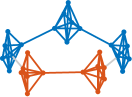
(d)

Figure 1: The Fiedler cuts on four graphs: the 4-dimensional hypercube $G_{\textrm{cube}(4)}$ in (a), the buckyball $G_{\rm buckyball}$ in (b), the cylindrical mesh $G_{P\mathbin{\text{\scalebox{0.84}{$\square$}}}C(10,10)}$ in (c) and the ring of cliques $G_{\textrm{RoK}(6,5)}$ in (d). The nodes on each graph are homogeneous or nearly homogeneous. On each graph, the subgraphs by a Fiedler cut are shown in two different colors. The modularity maximization at $\gamma=1$ favors the Fiedler cut over no-cut on each of the graphs. Detailed descriptions and information on the graphs are in Section III and in Table 1

Hypercube $G_{\textrm{cube}(k)}$, of dimension $k>2$. The graph has $2^{k}$ nodes with regular degree $k$, as illustrated in LABEL:fig:fiedler-cut-plots:cube. Unequivocally, the hypercube is not to be decoupled. The Fiedler value $\lambda_{2}$ of $G_{\textrm{cube}(k)}$ is equal to $2/k$ with multiplicity $k$. By Theorem 1, $\beta_{\max}=1-\lambda_{2}>0$ and there are many different Fiedler cuts. Any $u_{\max}$ is in the Fiedler space of dimension $k$ and induces a cut to the hypercube. Let $s={\rm sign}(u_{\max})$. One can verify that $Q(s\!\mid\!B)=s^{\rm T}Bs>0$. In particular, one of the Fiedler cuts leads to two subcubes of dimension $k\!-\!1$, see a Fiedler cut of $G_{\textrm{cube}(4)}$ illustrated in LABEL:fig:fiedler-cut-plots:cube. The modularity value $Q$ at this cut is $(k\!-\!2)/(2k)$, greater than the value at the all-in-one configuration $\Omega_{\vee}$, $Q(\Omega_{\vee})=0$. The modularity maximization thereby favors any of the Fiedler cuts over no-cut, falsely.

Buckyball $G_{\textrm{buckyball}}$  (Molecule $C_{60}$). The graph has $60$ nodes with regular degree $3$, as shown in LABEL:fig:fiedler-cut-plots:buckyball. The Fiedler value $\lambda_{2}$ of the buckyball is of multiplicity $3$, analytically. Numerically, $\lambda_{2}\approx 0.081$, much smaller than $1$. Thus, any maximum eigenvector $u_{\max}$ of $\hat{B}$ is in the Fiedler space of dimension $3$, and induces a cut to the Buckyball graph. The modularity value at such a cut is 0.39, greater than zero at $\Omega_{\vee}$.

Cylindrical mesh $G_{P\mathbin{\text{\scalebox{0.84}{$\square$}}}C(p,q)}$. The mesh is the Cartesian product of the $p$-nodes path graph and the $q$-nodes cycle graph, i.e., $G_{P\mathbin{\text{\scalebox{0.84}{$\square$}}}C(p,q)}=P_{p}\mathbin{\text{\scalebox{0.84}{$\square$}}}C_{q}$. Although its nodes have nearly homogeneous connection structures, the mesh is subject to a cut by the modularity maximization because $\lambda_{2}<1$. The cut is unique as $\lambda_{2}$ is simple. The cylindrical mesh $G_{P\mathbin{\text{\scalebox{0.84}{$\square$}}}C(10,10)}$ with the cut is illustrated in LABEL:fig:fiedler-cut-plots:mesh. For $G_{P\mathbin{\text{\scalebox{0.84}{$\square$}}}C(10,10)}$, $\lambda_{2}\approx 0.027$, much smaller than $1$. The modularity $Q$-value at the Fiedler cut is 0.447, greater than zero at $\Omega_{\vee}$.

IV The critical transition value

Among other approaches to overcoming the resolution limit, Reichardt and Bornholdt introduced the resolution parameter $\gamma$ [11], using the expression (3),

$$Q(\Omega\mid\gamma)=\sum_{C\in\Omega}\alpha(C,C)-\gamma\,\alpha^{2}(C,V),\quad\quad\gamma>0.$$ (11)

This $\gamma$-parametrized model is known as the generalized modularity model. Roughly speaking, a smaller $\gamma$ value promotes coarser clusters, whereas a larger $\gamma$ value advocates finer clusters.

For cluster configurations with at most two clusters, the parametrized model can be written in quadratic forms similar to those in (6) and (7). We parametrize the prime and standard modularity matrices $B$ and $\hat{B}$, respectively, as follows,

$$B(\gamma) =A-\gamma\,d\,d^{\rm T},$$ (12)

$$\hat{B}(\gamma) =D^{-1/2}B(\gamma)D^{-1/2}$$

$$=(I-L)-\gamma\,d^{1/2}\,(d^{1/2})^{\rm T},$$

where $L$ is the normalized graph Laplacian. Using the same notation and derivation as in the preceding sections, we have

$$Q(s\!\mid\!B(\gamma)) =\frac{1}{2}\left(s^{\rm T}B(\gamma)\,s+(1-\gamma)\right),$$ (13)

$$\phantom{xxx}s\in\{1,-1\}^{n}.$$

and

$$2\,Q(\,y(s)\!\mid\!\hat{B}(\gamma)) =y(s)^{\rm T}\hat{B}(\gamma)\,y(s)+(1-\gamma),$$ (14)

$$y(s) =D^{1/2}s,\quad s\in\{1,-1\}^{n}.$$

We provide in Appendix A a detailed proof of (13). As $y(s)$ is fittingly on the unit sphere $S$, we extend the discrete support of $Q$ to $S$,

$$u_{\max} =\arg\max_{u\in S}R(\,u\!\mid\!\hat{B}(\gamma)),$$ (15)

$$\phantom{xx}R(\,u\!\mid\!\hat{B}(\gamma))=u^{\rm T}\hat{B}(\gamma)\,u.$$

We generalize Theorem 1 from the particular case of $\gamma=1$ to arbitrary values of the resolution parameter $\gamma$.

Theorem 2.

Let $\hat{B}(\gamma)$ be the $\gamma$-parametrized standard modularity matrix as defined in (12), $\gamma>0$. Let $\lambda_{i}$ and $\beta_{\max}$ be specified as in Theorem 1. Then, the following hold true.

1. The eigenvalues of $\hat{B}(\gamma)$ are $\{1-\gamma\}\cup\{1\!-\!\lambda_{i},i=2,\dots,n\}$. The corresponding eigenvectors of $\hat{B}(\gamma)$ are the Laplacian eigenvectors associated with $\lambda_{i}$, $i=1,2,\!\dots,\!n$, respectively, and therefore $\gamma$-independent.

2. The largest eigenvalue of $\hat{B}(\gamma)$ depends on $\gamma$,

   $$\beta_{\max}=\max\{1-\gamma,1-\lambda_{2}\}.$$ (16)

   Any eigenvector $u_{\max}$ associated with $\beta_{\max}$ is characterized as follows,

   1. Case $\gamma<\lambda_{2}$: $\beta_{\max}=1-\gamma$, $u_{\max}=d^{1/2}>0$, and $u_{\max}$ is unique.

   2. Case $\gamma>\lambda_{2}$: $\beta_{\max}=1-\lambda_{2}$, $u_{\max}$ is orthogonal to $d^{1/2}$, $e^{\rm T}d^{1/2}=0$, and specifically, $u_{\max}\in{\rm span}\{u\mid Lu=\lambda_{2}u\}$. The maximum vector is unique if and only if $\lambda_{2}$ is simple.

   3. Case $\gamma=\lambda_{2}$: $\beta_{\max}=1-\lambda_{2}=1-\gamma$, and $u_{\max}\in{\rm span}\{d^{1/2},u\mid Lu=\lambda_{2}u\}$, i.e., $u_{\max}$ is in the invariant subspace of $L$ associated with $\lambda_{1}$ and $\lambda_{2}$. The elements of $u_{\max}$ either have the same sign or have mixed signs.

We revisit the graphs $G_{\rm cube(k)}$, $G_{\rm buckyball}$ and $G_{P\mathbin{\text{\scalebox{0.84}{$\square$}}}C(p,q)}$, which are described in Section III and illustrated in Fig. 1. For each of the graphs, the Fiedler value $\lambda_{2}$ is less than $1$, and by Theorem 2, the $\gamma$-value shall be set less than $\lambda_{2}$. At the all-in-one configuration $\Omega_{\vee}$, we have $Q(\Omega_{\vee}\mid\gamma)=1-\gamma$, which is equal to $\beta_{\max}$ when and only when $\gamma\leq\lambda_{2}$. For each graph, by setting $\gamma$ smaller than $\lambda_{2}$, the graph is kept in $\Omega_{\max}$ as a whole as expected. We conclude that the fault with the original modularity model lies in the fixed setting of $\gamma$ to $1$, oblivious and non-adaptive to graph structures.

Theorem 2 leads to the following revelation.

Theorem 3 (The critical transition at the Fiedler value).

For any undirected, connected graph $G$, the Fiedler value $\lambda_{2}$ is the critical value of the resolution parameter $\gamma$ in the following sense: when $\gamma<\lambda_{2}$, the maximum eigenvector of $\hat{B}(\gamma)$ is unique, its elements are of the same sign, not inducing any graph division; when $\gamma>\lambda_{2}$, the elements of any maximum eigenvector of $\hat{B}(\gamma)$ have mixed signs, inducing a graph split.

A few remarks are in order. For graph partitions with the minimum set of cut edges, the Fiedler value is a measure of the min-cut edge set relative to the volumes of the divided subgraphs. For graph clustering/community detection, by Theorem 3, the Fiedler value assumes an additional important role as the critical value of the resolution parameter $\gamma$ on its effect on the state of the optimum configuration $\Omega_{\max}(\gamma)$: with or without a graph division. The modularity spectral theory summarized in Theorems 2 and 3 advances our understanding of the resolution parameter $\gamma$ in the model (11). At the forefront, $\gamma$ regulates the policies regarding graph splits or merges. In the backend, the resolution parameter effectively modulates the maximum spectral value of $\hat{B}(\gamma)$.

The first two preponderant implications of the modularity spectral theory are immediate. (i) The $\gamma$-parametrized model at any fixed value of $\gamma$, $\gamma\neq 1$, inherits the very same flaw as in the case of $\gamma=1$: the maximum vectors of $\hat{B}(\gamma)$ indiscriminately induce Fiedler cuts on any graph with the Fiedler value $\lambda_{2}$ less than $\gamma$. (ii) If $\gamma$ is set greater than $2$, then a Fiedler cut is induced on any graph. Consider, for example, any clique $K_{n}$, including the edge graph $K_{2}$. The modularity $Q$ at $\gamma=2$ has a higher value at a Fiedler cut than the value at $\Omega_{\vee}$ without graph split. We will discuss in Section VII additional implications, some of which are subtle.

V The critical transition region

Table 1: The Fiedler value $\lambda_{2}$ and the Fiedler pseudo-set (FPS) descriptor $(t_{\min},t_{\max})$ for each of the $4$ small and structured graphs, Zachary’s karate club [21], and $2$ larger and random graphs on the table. The topological structures of the first four graphs are illustrated in Fig. 1. Two types of perturbations—edge removal ($r_{e}$) and edge rewiring ($r_{w}$)—at two levels are considered. At the first level, one edge is removed from or rewired on each small graph; $1\%$ of the edges, on each large graph. At the second perturbation level, two edges are removed from or rewired on each small graph; $2\%$ of the edges, on each large graph. For each case, the FPS is estimated by $100$ trials. See more detailed descriptions in Section V.

				$r_{w}=1$		$r_{e}=1$		$r_{w}=2$		$r_{e}=2$
Graph		$\lambda_{2}$	$\lambda_{3}$	$t_{\min}$	$t_{\max}$	$t_{\min}$	$t_{\max}$	$t_{\min}$	$t_{\max}$	$t_{\min}$	$t_{\max}$
Cylindrical mesh	$P\mathbin{\text{\scalebox{0.84}{$\square$}}}C(33,3)$	$0.002$	$0.009$	$\nicefrac{{1}}{{1.01}}$	$\nicefrac{{3.99}}{{1}}$	$\nicefrac{{1}}{{1.05}}$	$\nicefrac{{1.01}}{{1}}$	$\nicefrac{{1}}{{1.03}}$	$\nicefrac{{5.72}}{{1}}$	$\nicefrac{{1}}{{1.09}}$	$\nicefrac{{1.02}}{{1}}$
Ring of cliques	$\textrm{RoK}(6,17)$	$0.003$	$0.003$	$\nicefrac{{1}}{{3.85}}$	$\nicefrac{{1}}{{1.00}}$	$\nicefrac{{1}}{{3.95}}$	$\nicefrac{{1.00}}{{1}}$	$\nicefrac{{1}}{{3.91}}$	$\nicefrac{{2.41}}{{1}}$	$\nicefrac{{1}}{{\infty}}$	$\nicefrac{{1.01}}{{1}}$
Buckyball	$(n=60\phantom{6},m=90)$	$0.081$	$0.081$	$\nicefrac{{1}}{{1.16}}$	$\nicefrac{{1}}{{1.01}}$	$\nicefrac{{1}}{{1.14}}$	$\nicefrac{{1}}{{1.10}}$	$\nicefrac{{1}}{{1.41}}$	$\nicefrac{{1}}{{1.01}}$	$\nicefrac{{1}}{{1.37}}$	$\nicefrac{{1}}{{1.09}}$
Hypercube	$\textrm{Cube}(8)$	$0.250$	$0.250$	$\nicefrac{{1}}{{1.01}}$	$\nicefrac{{1}}{{1.01}}$	$\nicefrac{{1}}{{1.01}}$	$\nicefrac{{1}}{{1.01}}$	$\nicefrac{{1}}{{1.02}}$	$\nicefrac{{1}}{{1.01}}$	$\nicefrac{{1}}{{1.02}}$	$\nicefrac{{1}}{{1.01}}$
Zachary’s karate club	$(n=34\phantom{6},m=78)$	$0.132$	$0.287$	$\nicefrac{{1}}{{1.11}}$	$\nicefrac{{1.30}}{{1}}$	$\nicefrac{{1}}{{1.18}}$	$\nicefrac{{1.06}}{{1}}$	$\nicefrac{{1}}{{1.20}}$	$\nicefrac{{1.46}}{{1}}$	$\nicefrac{{1}}{{1.18}}$	$\nicefrac{{1.07}}{{1}}$
				$r_{w}=1\%$		$r_{e}=1\%$		$r_{w}=2\%$		$r_{e}=2\%$
Erdös-Rényi	$\textrm{ER}(n=2000,\,\,d_{\textrm{avg}}=16)$	$0.519$	$0.523$	$\nicefrac{{1}}{{1.00}}$	$\nicefrac{{1.00}}{{1}}$	$\nicefrac{{1}}{{1.01}}$	$\nicefrac{{1}}{{1.00}}$	$\nicefrac{{1}}{{1.01}}$	$\nicefrac{{1.01}}{{1}}$	$\nicefrac{{1}}{{1.01}}$	$\nicefrac{{1}}{{1.01}}$
Barabási-Albert	$\textrm{BA}(n=2000,\,\,d_{\textrm{avg}}=16)$	$0.529$	$0.531$	$\nicefrac{{1}}{{1.01}}$	$\nicefrac{{1.00}}{{1}}$	$\nicefrac{{1}}{{1.01}}$	$\nicefrac{{1}}{{1.00}}$	$\nicefrac{{1}}{{1.01}}$	$\nicefrac{{1.00}}{{1}}$	$\nicefrac{{1}}{{1.02}}$	$\nicefrac{{1}}{{1.00}}$

If the Fiedler value $\lambda_{2}$ is relatively smaller than $\mbox{\rm trace}(L)/(n-1)$, which is the average of the non-zero Laplacian, it signifies a meaningful graph partition, or indicates a possible cluster configuration with more than one clusters. There is, however, a crucial distinction between graph partition and graph clustering: a small value of $\lambda_{2}$ is insufficient to ascertain the presence of more than one clusters/communities. For a case in point, consider the RoK graph $G_{\textrm{RoK}(6,17)}$ and the cylindrical mesh $G_{P\mathbin{\text{\scalebox{0.84}{$\square$}}}C(33,3)}$, both are shown in Fig. 1. The two graphs have about the same number of nodes, and their Fiedler values are small and comparable, see Table 1. Despite having a smaller Fiedler value, the cylindrical mesh shall not be split, whereas each clique in the RoK graph is seen as a closely tied community. The Fiedler values alone are insufficient to spell out the difference in connectivity between these two graphs.

We define the Fiedler pseudo-set (FPS) of a graph $G$, with respect to a tolerance threshold $\varepsilon>0$, as follows,

$$\Lambda_{2}(A,\varepsilon)=\big{\{}\,\lambda_{2}\!\mid L(A+E)u=\lambda_{2}u,\,\|E\|\leq\varepsilon\|A\|\,\big{\}},$$ (17)

where $L$ is the normalized graph Laplacian, $E$ represents a perturbation or change in $A$, and $\|\cdot\|$ is a matrix norm. One may impose certain constraints on the perturbation matrix $E$, such as by a probabilistic model, or by domain-specific knowledge. The FPS measures the variation in the Fiedler value, i.e., the network connectivity, in response to small changes in a graph due to random perturbation, editing, or rewiring.

Graph $G$ is said $\varepsilon$-stable in connectivity if the dispersion of $\lambda_{2}$ in $\Lambda_{2}$ is relatively small. When $\lambda_{2}$ is small, an $\varepsilon$-stable graph is resistant to division. Among many possible ways to measure the sensitivity of a network connectivity, we may simply use the pair of ratios $t_{\min}=\min(\Lambda_{2})/\lambda_{2}$ and $t_{\max}=\max(\Lambda_{2})/\lambda_{2}$. If $\lambda_{2}$ is small and $\min(\Lambda_{2})$ is much smaller, then the graph tends to break apart.

By the measure of connection sensitivity, we are able to definitively and quantitatively differentiate the RoK graph $G_{\textrm{RoK}(6,17)}$ and the cylindrical mesh $G_{P\mathbin{\text{\scalebox{0.84}{$\square$}}}C(33,3)}$ mentioned above. We show in Table 1 that for the RoK graph, $\min(\Lambda_{2})$ becomes $4$ times smaller when one edge is removed or rewired, and it becomes zero when two edges are removed or rewired. This reveals the tendency of the RoK graph to break apart. In contrast, the cylindrical mesh is stable while undergoing similar changes, the ratio $t_{\min}$ is close to $1$, signifying a strong bond within the graph to stay as a whole. Based on this analysis, we reach conclusions that are in line with our heuristic understanding of these graphs. We may say that the sensitivity analysis gives foundational support to our intuitive understanding of the community structure on a RoK graph. The FPS provides reliable information, which cannot be contained in a single Fiedler value, for making robust decisions in a community detection process.

The FPS has broader theoretical and practical merits.

(i) The FPS is the connectivity characteristic for complex network. It acknowledges and regards the typical co-existence of structures and randomness in a complex network and measures their interplay. The randomness in a complex network defies connectivity description by the Fiedler value at a single random instantiation. (ii) In the context of the $\gamma$-setting with the modularity model, the FPS is the critical region, in place of the single value $\lambda_{2}$ in Theorem 3. The larger the dispersion in $\Lambda_{2}$ from $\lambda_{2}$ is, the more uncertainty is in the transition between division and no-division configuration states. This critical region transcends the critical transition analysis in Section IV. (iii) The FPS can be used to assess the robustness of an inferred community configuration, in combination with other existing measures [22]. (iv) When a complex network is stable in connectivity, by the FPS, its community structure can be inferred reliably from a particular instantiation. This includes the analysis of subnetwork structures in Section VI. (v) The structure of the subspace associated with the FPS can be used to explain or help resolve some other ambiguity or uncertainty issues related to graph clustering/community detection. We describe such a scenario in Section VII.

We show in Table 1 the Fiedler values and the Fiedler pseudo-sets for several graphs, including a Barabási-Albert (BA) graph [2] and an Erdös-Rényi (ER) graph [23, 24], each with $2000$ nodes and degree $16$ on average. The Fiedler values for the BA graph and the ER graph are far from small, and they do not disperse much in their Fiedler pseudo-sets. These findings align well with the existing understanding that BA and ER graphs typically lack clear and distinct community structures. Except for the RoK graph, the other graphs on Table 1 are also stable in connectivity when subject to similar changes.

For the experimental results in Table 1, the Fiedler pseudo-set $\Lambda_{2}(\varepsilon)$ for each graph is estimated by $\min\{m,100\}$ random trials of edge removal or rewiring, $m$ is the total number of edges on the graph.

VI The sub-modularity matrix

Many search algorithms for modularity maximization leverage a highly attractive property, the separability, of the function $Q(\Omega\mid\gamma)$ at any fixed value of the resolution parameter $\gamma$ [25, 26]. Let $V_{1}$ be a subset of vertices. Let $H$ be the subgraph induced by $V_{1}$. Denote by ${V}_{2}$ the complement of $V_{1}$ in $V$. Let $H^{c}$ be the subgraph induced by $V_{2}$. At some algorithmic steps, the search operations can be restricted to $H$ while the rest of the graph is fixed or undergoes changes independently:

$$Q(\Omega\mid\gamma) =\sum_{C_{i}\subset\Omega(V_{1})}\alpha(C_{i},C_{i})-\gamma\,\alpha^{2}(C_{i},V)$$ (18)

$$\phantom{xx}+\sum_{C_{j}\subset\Omega(V_{2})}\alpha(C_{j},C_{j})-\gamma\,\alpha^{2}(C_{j},V).$$

We introduce the augmented graph $\bar{H}$ obtained from $G$ by joining $H$ and a graph minor of $H^{c}$. Suppose $H^{c}$ has a cluster structure $\{C_{j}\}$, each cluster $C_{j}$ is connected. By contracting each $C_{j}$ into a single node, we get a graph minor of $H^{c}$. We detail the basic case that the entire $H^{c}$ is contracted to a single node. For clarity, we describe the augmented graph $\bar{H}$ by its adjacency matrix $\bar{A}_{1}$,

$$\bar{A}_{1}=\left(\begin{array}[]{cc}A(V_{1},V_{1})&A(V_{1},V_{2})\,e\\ e^{\rm T}A(V_{2},V_{1})&0\end{array}\right)$$ (19)

The leading matrix $A(V_{1},V_{1})$ is the adjacency matrix of the subgraph $H$. The last column (row) of $\bar{A}_{1}$ is associated with the augmented node $\bar{v}$, which represents the existence of all other nodes external to $H$. The number of the nonzero elements in the column is the number of edges between $V_{1}$ and $\bar{v}$. For any $v_{i}\in V_{1}$, $A(v_{i},V_{2})e$ is the weight on the edge between $v_{1}$ and $\bar{v}$, equal to the sum of the connection weights between node $v_{i}$ and all nodes in $V_{2}$. For the extreme case that $H$ has a single vertex $v_{i}$, the extended graph $\bar{H}$ is the edge graph with $v_{i}$ and $\bar{v}$, the edge weight is equal to $d(v_{i})$. For the other extreme case that $H$ has $(n-1)$ nodes, $\bar{A}_{1}=A$, i.e., the augmented graph is $G$.

When graph $H^{c}$ has a configuration of $k$ clusters $\{C_{j},j=1,\dots,k\}$, $k>1$, it can be represented by a $k$-nodes graph minor obtained by cluster contraction. Then, graph $H$ is augmented to $\bar{H}$ by $k$ external nodes/graph minor nodes. The external nodes are intra-linked and weighted by the edges in the graph minor, and they are linked to the nodes in $V_{1}$ by the interconnections $\alpha(v_{i},C_{j})$, $v_{i}\in V_{1}$ and $C_{j}$ is a cluster of $H^{c}$.

The augmented graph $\bar{H}$ has the following properties. (i) It preserves the interconnection between $H$ and $H^{c}$. As long as $G$ is connected, the augmented graph $\bar{H}$ is connected, regardless of the granularity of a graph minor for representing $H^{c}$. (ii) It also preserves the probabilistic transition among the nodes in $V_{1}$. For any vertex $v_{1}$ in $V_{1}$, its volume/degree $d(v_{i})$ on $G$ is preserved on $\bar{H}$. Denote by $\bar{d}_{1}$ the degree vector on $\bar{H}$, $\bar{d}_{1}=\bar{A}_{1}e$. Then, $\bar{d}_{1}(v_{i})=d(v_{i})$, $v_{i}\in V_{1}$. Let $\bar{D}_{1}=\mbox{\rm diag}(\bar{d}_{1})$. By the comparison between the two stochastic matrices $\bar{A}_{1}\bar{D}_{1}^{-1}$ and $AD^{-1}$, the probabilistic transition from node $v_{i}$ in $V_{1}$ to any other node $v_{j}$ in $V_{1}$ on $\bar{H}$ remains the same as that on $G$. (iii) We can apply the $\gamma$-parametrized modularity model to the augmented graph $\bar{H}$. By the separability of the modularity function (18) and the properties of $\bar{H}$, at any value of $\gamma$ ($\bar{H}$ is independent of $\gamma$), an ascending/descending of $Q$ on $\bar{H}$ implies directly the same amount of ascending/descending of $Q$ on $G$. If the maximal $Q$-value is at the no-partition of $\bar{H}$ or at the partition between $V_{1}$ and the augmented nodes, then no independent division of $H$ improves the modularity value, which implies a merge decision if $H$ results from a union of more than one inter-connected subgraphs.

We are in a position to describe the $\gamma$-parametrized modularity matrix $\hat{B}$ for $\bar{H}$,

$$\hat{B}_{1}\left(\gamma\right)=\left(I-L(\bar{H})\right)-\frac{\gamma}{e^{\rm T}\bar{d}_{1}}\,\bar{d}_{1}^{1/2}\left(\bar{d}_{1}^{1/2}\right)^{\rm T},$$ (20)

where $\bar{d}_{1}=\bar{A}_{1}e$ is the degree vector on $\bar{H}$, $L(\bar{H})$ is the normalized Laplacian of graph $\bar{H}$. The formulation of (20) is computation-friendly, scaling the degree vector only without scaling the entire matrix $\bar{A}_{1}$, because the Laplacian is invariant to scaling in $\bar{A}_{1}$.

The theory on the spectral structure of the parametrized modularity matrix $\hat{B}(\gamma)$ holds true for the augmented graph $\bar{H}$. Furthermore, all the above applies to any subgraph of $\bar{H}$, recursively, in adaption to the graph structure. This effectively extends the modularity spectral analysis to multi-community detection.

Additional comments. (1) The augmented nodes for external connections are necessary. Consider, for example, graph $G_{\rm 2stars}$, which has a single edge connecting two copies of a star graph with more than $3$ leaf nodes. Let $V_{1}$ be a subset of nodes with degree $1$. Then, the graph $H$ induced by $V_{1}$ is composed of isolated nodes. In contrast, with the augmented node $\bar{v}$ contracted from $H^{c}$, $\bar{H}$ is a star graph, all nodes in $V_{1}$ are attached to $\bar{v}$. (2) The granularity of a graph minor for representing $H^{c}$ affects the connectivity and cluster granularity on $\bar{H}$. Revisit the graph $G_{\rm 2star}$. We can contract $H^{c}$ to a graph minor with two nodes, each node is associated with the center of a star subgraph. If $V_{1}$ contains leaf nodes from both stars, then $\bar{H}$ is also a two-star graph. As a matter of fact, the augmented subgraphs are used in both modularity model analysis and practical search algorithms for modularity maximization [25, 26].

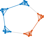
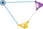
			$r_{w}=1$		$r_{e}=1$		$r_{w}=2$		$r_{e}=2$
Graph	$\lambda_{2}$	$\lambda_{3}$	$t_{\min}$	$t_{\max}$	$t_{\min}$	$t_{\max}$	$t_{\min}$	$t_{\max}$	$t_{\min}$	$t_{\max}$
$G_{\textrm{RoK}}(6,5)$	$0.033$	$0.033$	$\nicefrac{{1}}{{3.47}}$	$\nicefrac{{1.00}}{{1}}$	$\nicefrac{{1}}{{3.61}}$	$\nicefrac{{1.00}}{{1}}$	$\nicefrac{{1}}{{3.37}}$	$\nicefrac{{1.54}}{{1}}$	$\nicefrac{{1}}{{\infty}}$	$\nicefrac{{1.02}}{{1}}$
$\bar{H}_{\textrm{red}}$	$0.079$	$0.716$	$\nicefrac{{1}}{{2.12}}$	$\nicefrac{{1.70}}{{1}}$	$\nicefrac{{1}}{{2.79}}$	$\nicefrac{{1.04}}{{1}}$	$\nicefrac{{1}}{{1.67}}$	$\nicefrac{{2.46}}{{1}}$	$\nicefrac{{1}}{{\infty}}$	$\nicefrac{{1.08}}{{1}}$

Figure 2: Left: The ring-of-clique (RoK) graph $G_{\textrm{RoK}(6,5)}$ and its division into two subgraphs $H_{\rm blue}$ and $H_{\rm red}$ in red and blue, respectively. The Fiedler value of $G_{\rm RoK(6,5)}$ is of multiplicity $2$ and relatively small to the average of the Laplacian values, It decreases with one edge removal/rewiring and becomes zero with two-edges removal/rewiring. Right. The augmented graph $\bar{H}_{\rm red}$ and the further split of $H_{\rm red}$ into two subgraphs in purple and yellow, respectively. The circled blue node denotes the contracted graph $H_{\rm blue}$. The two edges between $H_{\rm blue}$ and $H_{\rm red}$ are maintained in $\bar{H}_{\rm red}$. The Fiedler value of $\bar{H}_{\rm red}$ is simple and small. It decreases with one-edge removal/rewiring and becomes zero with two-edges removal/rewiring.

We show in Fig. 2 the RoK graph $G_{\textrm{RoK}(6,5)}$, its division into two subgraphs $H_{\rm red}$ and $H_{\rm blue}$, and the augmented graph $\bar{H}_{\rm red}$. The augmented graph $\bar{H}_{\rm red}$ has the external node $\bar{v}$ (annotated by the circled blue marker) and maintains the two edges between $H_{\rm blue}$ and $H_{\rm red}$. The Fiedler value of $G_{\rm RoK(6,5)}$ is relatively small compared to the average $n/(n-1)$ ($n=30$) of the Laplacian values for the graph. Furthermore, by the FPS descriptor $t_{\min}=\min(\Lambda_{2})/\lambda_{2}$, the Fiedler value becomes $3$ times smaller over one-edge removal/rewiring, and becomes $0$ over two-edges removal. The division of $G_{\textrm{RoK}(6,5)}$ into $H_{\rm red}$ and $H_{\rm blue}$ is justified. By similar arguments, the split of $\bar{H}_{\rm red}$ is certified.

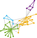
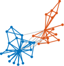
			$r_{w}=1$		$r_{e}=1$		$r_{w}=2$		$r_{e}=2$
Graph	$\lambda_{2}$	$\lambda_{3}$	$t_{\min}$	$t_{\max}$	$t_{\min}$	$t_{\max}$	$t_{\min}$	$t_{\max}$	$t_{\min}$	$t_{\max}$
$G_{\textrm{karate}}$	$0.132$	$0.287$	$\nicefrac{{1}}{{1.11}}$	$\nicefrac{{1.30}}{{1}}$	$\nicefrac{{1}}{{1.18}}$	$\nicefrac{{1.06}}{{1}}$	$\nicefrac{{1}}{{1.20}}$	$\nicefrac{{1.46}}{{1}}$	$\nicefrac{{1}}{{1.18}}$	$\nicefrac{{1.07}}{{1}}$
$\bar{H}_{\textrm{blue}}$	$0.379$	$0.419$	$\nicefrac{{1}}{{1.20}}$	$\nicefrac{{1.10}}{{1}}$	$\nicefrac{{1}}{{1.17}}$	$\nicefrac{{1.08}}{{1}}$	$\nicefrac{{1}}{{1.23}}$	$\nicefrac{{1.15}}{{1}}$	$\nicefrac{{1}}{{1.27}}$	$\nicefrac{{1.12}}{{1}}$
$\bar{H}_{\textrm{red}}$	$0.235$	$0.705$	$\nicefrac{{1}}{{1.31}}$	$\nicefrac{{1.40}}{{1}}$	$\nicefrac{{1}}{{1.30}}$	$\nicefrac{{1.11}}{{1}}$	$\nicefrac{{1}}{{1.36}}$	$\nicefrac{{1.68}}{{1}}$	$\nicefrac{{1}}{{1.78}}$	$\nicefrac{{1.19}}{{1}}$

Figure 3: Left: Zahary’s karate club graph [21] is divided into four communities by the modularity model at $\gamma=1.0$. Right: The same graph is split into two subgraphs, $H_{\rm blue}$ in blue and $H_{\rm red}$ in red, by the Fiedler vector of the club graph. The table provides the Fiedler values and the FPS descriptors $(t_{\min},t_{\max})$ for the club graph, the augmented subgraph $\bar{H}_{\rm red}$ and the augmented subgraph $\bar{H}_{\rm blue}$.

In Fig. 2, we show Zahary’s karate club graph [21] and two different community configurations. The configuration with four communities is by the modularity maximization at $\gamma=1$. The configuration with two communities is by the Fiedler spectral information of the graph and the two (augmented) subgraphs by the Fiedler cut. The Fiedler values of the subgraphs become much larger, they do not decrease much by random removal/rewiring of one or two edges.

Our analysis and experimental results have shown that the Fiedler values of (augmented) subgraphs vary from each other and from the Fiedler value of graph $G$. This brings to light another issue that the $\gamma$-setting also affects subgraph split or merge decisions, consequently, the recognition or misidentification of sub-community structures.

VII Discussion

Recall the standard modularity matrix $\hat{B}(\gamma)$ as defined in (12). The modularity spectral analysis across the variation of the resolution parameter $\gamma$ presented in the preceding sections is grounded in two key connections that we have established. First, we identify the $\gamma$-parametrized modularity function $Q(\Omega\!\mid\!\gamma)$ over all possible binary graph partitions with the quadratic expression $y^{\rm T}\hat{B}(\gamma)y$ over the discrete set $Y=\{y\mid y=D^{1/2}s,s=\{1,-1\}^{s}\}$. Secondly, as the discrete set $Y$ is fittingly embedded within the unit sphere $S=\{u\mid u^{\rm T}u=1\}$, the quadratic expression of the modularity function $Q$ can be readily extended to its continuous counterpart, the Rayleigh quotient $R(u\mid\hat{B}(\gamma))$ on the sphere $S$. Understanding $R(u\!\mid\!\hat{B}(\gamma))$ gives us invaluable insights into the modularity maximization. The behavior and properties of $R(u\mid\hat{B}(\gamma))$ on the sphere $S$ can be entirely determined by the spectral structure of the kernel matrix $\hat{B}(\gamma)$.

Our modularity spectral analysis offers a unique perspective on the relationship between the graph spectral structure and the modularity spectral structure. In a nutshell, the entire Laplacian spectral structure is in the modularity matrix $\hat{B}(\gamma)$, across all variations in $\gamma$. Roughly speaking, while every Laplacian vector is a scalar (heat) map over the vertex set at a specific Laplacian eigenvalue (energy level), a maximum eigenvector of $\bar{B}(\gamma)$ induces a community map of the graph/network.

We have uncovered that every maximum eigenvector of the modularity matrix $\hat{B}(\gamma)$, $\gamma>0$, lies in the invariant subspace of the normalized graph Laplacian $L(G)$ associated with the two smallest Laplacian eigenvalues: $\lambda_{1}=0$ and $\lambda_{2}>0$. When $\gamma\neq\lambda_{2}$, the maximum vectors of the modularity matrix $\hat{B}(\gamma)$ are either in the null space of $L(G)$ or in the Fiedler space as defined in Section II. We provide a few more comments below.

(A) The proxy criteria & configuration candidates. The Fiedler connection analysis not only provides profound insights into the behaviors and properties of the modularity model and the maximization process, it also promises a potential impact on the development of effective criteria for $\gamma$-setting as well as for efficient algorithmic search of maximal-modularity configurations. Specifically, we may use the Fiedler value $\lambda_{2}$ and the Fiedler pseudo-set $\Lambda_{2}(\varepsilon)$ of a graph, or a subgraph, to assess the merge or split results at a specified $\gamma$ value and provide valuable feedback for adaptive $\gamma$-setting. Subsequently, the maximum vectors of matrix $\hat{B}(\gamma)$ propose configuration candidates. All maximum vectors reside in the null space or/and the Fiedler space. Computationally, the eigenvector associated with the zero eigenvalue of the Laplacian is unique and it is $d^{1/2}$, readily available. The Fiedler value $\lambda_{2}$ can be easily obtained numerically. If $\lambda_{2}$ is simple, the Fiedler vector is unique, and it is also easily obtainable. In practice, the Fiedler vectors have long been used in spectral clustering algorithms for image segmentation and some other domain-specific graph clustering applications, and the search over a continuous domain is combined with the search over a discrete domain [27, 28]. (B) The Fiedler space & graph symmetry. When the Fiedler space is dominant in $\hat{B}(\gamma)$ and multi-dimensional, the variety in graph division is great and not to be overlooked. The existence of many different Fiedler cuts on the same graph indicates the presence of homogeneous or symmetric substructures in the graph. Consider a few particular graphs with symmetric structures – $K_{n}$, $G_{\rm cube(k)}$, and $G_{\rm buckyball}$. The multiplicity of $\lambda_{2}$ reaches the highest at $(n\!-\!1)$ for the clique $K_{n}$, it is equal to $k$ for the $k$-dimensional hypercube, and equal to $3$ for the buckyball $G_{\rm buckyball}$. Although none of these specific graphs with symmetric structures, $K_{n}$, $G_{\rm cube(k)}$, $G_{\rm buckyball}$ and $G_{P\mathbin{\text{\scalebox{0.84}{$\square$}}}C(p,q)}$, should be divided, the presence of symmetric structures does not preclude the possibility of identifying meaningful graph splits. Consider, for instance, the RoK graph, $G_{\textrm{RoK}(p,q)}$, $p,q>4$. The multiplicity of its Fiedler value is greater than one, reflecting, indeed, the symmetric substructures. However, each clique $K_{p}$ in $G_{\textrm{RoK}(p,q)}$ is certified as a closely tied community/cluster, as we have discussed in Sections V and VI. The multiplicity of the Fiedler value highlights the broader phenomena where $\lambda_{2}$, which may be simple, is followed closely by $\lambda_{3}$ or more than one other eigenvalues. For instance, the Fiedler value of the cylindrical mesh $G_{P\mathbin{\text{\scalebox{0.84}{$\square$}}}C(p,q)}$ is simple, and it is tightly followed by the other eigenvalues. Such spectral cluster phenomena indicate (nearly) homogeneous or symmetric substructures within a graph. The important message is this. The spectral cluster at the Fiedler value, if not sensitive to pertrubation, signifies the strength in bounding. When the Fiedler value is small, the graph is thin and strong like a graphene mesh. This finding raises the new issue on the community bounding strength, in addition to the issue with community size/resolution. The answer is again in the Fiedler pseudo-set $\Lambda_{2}$. There are other complicated issues when the Fiedler space is dominant and multi-dimensional. All maximum vectors of $\hat{B}$ arrive at the same maximal value $\beta_{\max}$ of the continuous quadratic function $u^{\rm T}\hat{B}(\gamma)\,u$. However, their sign indicators are not necessarily equal in the modularity value, $y(s)^{\rm T}\hat{B}(\gamma)\,y(s)=s^{\rm T}B(\gamma)s$, with $s=\mbox{\rm sign}(u)$. Ideally, we would like to locate a unit-length maximum vector with the maximal value of $u^{\rm T}y({\rm sign}(u))$, the similarity between $u$ and its counterpart $y(\mbox{\rm sign}(u))$. Computationally, an eigenvector(s) associated with the $\min(\Lambda_{2}(\varepsilon))$, with an $\varepsilon$-departure from the symmetry would help single out a good candidate configuration among innumerably many incidental combinations. This configuration would significantly reduce the combinatorial search cost.

• (C) Resolution parameter variation.By our analysis, it is necessary to consider the consistency and the variation of the maximum cluster configurations in response to changes in $\gamma$. Using the modularity model with a single value of $\gamma$, or even a narrow range of $\gamma$-values, is limited in detecting community structures with more than one heterogeneous communities. It is recently reported in [29, 26, 30, 25, 31] that a network with stable distinctive community structures is affiliated with more than one $\gamma$ regions, each region signifying the dominance of a cluster configuration at an intrinsic level of cluster granularity. • (D) Model transformation.With its beautiful simplicity and other attractive properties, the $\gamma$-parametrized modularity model remains broadly deployed, among many other existing models, for community detection. Our analysis exposes notwithstanding an inherent restriction within the framework across the entire $\gamma$-variation. Specifically, the spectral modulation mechanism affected by the modularity matrix $\hat{B}(\gamma)$ is constrained to the choice between the Fiedler space and the null space of the graph Laplacian. The finer structures are captured by other eigenvectors at the lower end of the Laplacian spectrum. It is not inconceivable to relax or remove the constraint without confining ourselves to the use of divide-and-conquer hierarchies. It is possible to modulate or reshape the model structure over a range of the graph spectrum beyond the two smallest eigenvalues, $\{\lambda_{1},\lambda_{2}\}$, with respect to a particular class of graphs of interest. The normalized Laplacian spectral structure decomposition is identified with the generalized eigenvalue problem $Ax=\lambda Dx$. The graph structures may also be analyzed or characterized by the generalized eigenvalue problem with a different symmetric, positive definite mass matrix $M$, $Ax=\lambda Mx$, or even a non-linear generalized eigenvalue problem [32, 33]. It is likely that existing, emerging, and competing models for community detection could be interpreted as different spectral modulation mechanisms.

Appendix A Quadratic form of modularity cuts

Proof of (13).

Denote by $e(C)$ the vector that is constant $1$ with length $|C|$, $C\subset V$. For any configuration $\Omega$ with two clusters, $\Omega=\{C_{1},C_{2}\}$, the adjacency matrix can be reordered so that

$$A=\left(\begin{array}[]{cc}A_{11}&A_{12}\\ A_{21}&A_{22}\end{array}\right),\quad A_{ij}=A(C_{i},C_{j}),\quad i,j=1,2.$$

The indicator of $\Omega$ can then be described as follows,

$$s^{\rm T}(\Omega)=[e^{\mathrm{T}}(C_{1}),\,-e^{\mathrm{T}}(C_{2})].$$

Assume that $e^{\rm T}Ae=1$. Then, the degree vector $d=Ae$ is stochastic. Let $d_{i}=d(C_{i})$, $i=1,2$. We have

$$s^{\mathrm{T}}(\Omega)B(\gamma)s(\Omega)=$$

$$\begin{bmatrix}e^{\mathrm{T}}(C_{1})&-e^{\mathrm{T}}(C_{2})\end{bmatrix}\begin{bmatrix}A_{11}-\gamma d_{1}d_{1}^{\mathrm{T}}&A_{12}-\gamma d_{1}d_{2}^{\mathrm{T}}\\[4.0pt] A_{21}-\gamma d_{2}d_{1}^{\mathrm{T}}&A_{22}-\gamma d_{2}d_{2}^{\mathrm{T}}\end{bmatrix}\begin{bmatrix}e(C_{1})\\[4.0pt] -e(C_{2})\end{bmatrix}.$$

Using the $\alpha$-notation of (4), we have $e^{\rm T}(C_{i})d(C_{i})=\alpha(C_{i},V)$, $i=1,2$. The two terms in $s^{\rm T}B(\gamma)s$ related to the diagonal blocks of $B(\gamma)$ sum to

$$\footnotesize\sum_{i=1,2}\alpha(C_{i},C_{i})-\gamma\alpha^{2}(C_{i},V)=Q(\Omega\mid\gamma).$$

The two terms related to the off-diagonal blocks of $B(\gamma)$ are equal to each other by the symmetry and sum to

$$2 \big{(}\gamma\,\alpha(C_{1},V)\alpha(C_{2},V)-\alpha(C_{1},C_{2})\big{)}$$

$$=\alpha(C_{1},C_{1})+\alpha(C_{2},C_{2})-\big{(}\underbrace{\alpha(C_{1},V)+\alpha(C_{2},V)}_{=1}\big{)}+$$

$$\phantom{=}+\gamma\big{(}\,\underbrace{\alpha(C_{1},V)+\alpha(C_{2},V)}_{=1}-\alpha^{2}(C_{1},V)-\alpha^{2}(C_{2},V)\,\big{)}$$

$$=Q(\Omega\mid\gamma)+\gamma-1,$$

where the following equalities are used

$$\alpha(C_{1},C_{2}) =\alpha(C_{2},C_{1}),$$

$$\alpha(C_{1},V) +\alpha(C_{2},V)=1,$$

$$\alpha(C_{1},C_{2}) =\alpha(C_{1},V)-\alpha(C_{1},C_{1})$$

$$=\alpha(C_{2},V)-\alpha(C_{2},C_{2}).$$

Thus, we have

$$Q(\Omega\mid\gamma)=\dfrac{1}{2}s^{\mathrm{T}}(\Omega)B(\gamma)s(\Omega)+\left(\dfrac{1-\gamma}{2}\right).$$

This equality extends to the all-in-one configuration $\Omega_{\vee}$ because $Q(\Omega_{\vee}\mid\gamma)=1-\gamma$. ∎

References

- de Solla Price [1965] D. J. de Solla Price, Networks of scientific papers, Science 149, 510 (1965).
- Barabási and Albert [1999] A.-L. Barabási and R. Albert, Emergence of scaling in random networks, Science 286, 509 (1999).
- Newman [2001] M. E. J. Newman, The structure of scientific collaboration networks, Proceedings of the National Academy of Sciences 98, 404 (2001).
- Girvan and Newman [2002] M. Girvan and M. E. J. Newman, Community structure in social and biological networks, Proceedings of the National Academy of Sciences 99, 7821 (2002).
- Newman [2006] M. E. J. Newman, Modularity and community structure in networks, Proceedings of the National Academy of Sciences 103, 8577 (2006).
- Rosvall and Bergstrom [2008] M. Rosvall and C. T. Bergstrom, Maps of random walks on complex networks reveal community structure, Proceedings of the National Academy of Sciences 105, 1118 (2008).
- Newman et al. [2011] M. Newman, A.-L. Barabási, and D. J. Watts, The Structure and Dynamics of Networks (Princeton University Press, Princeton, P.A., 2011).
- Barabási and Pósfai [2016] A.-L. Barabási and M. Pósfai, Network Science (Cambridge University Press, Cambridge, United Kingdom, 2016).
- Newman [2018] M. E. J. Newman, Networks, second edition ed. (Oxford University Press, Oxford, United Kingdom; New York, NY, United States of America, 2018).
- Fortunato and Barthelemy [2007] S. Fortunato and M. Barthelemy, Resolution limit in community detection, Proceedings of the National Academy of Sciences 104, 36 (2007).
- Reichardt and Bornholdt [2006] J. Reichardt and S. Bornholdt, Statistical mechanics of community detection, Physical Review E 74, 016110 (2006).
- Sheikholeslami et al. [1998] G. Sheikholeslami, S. Chatterjee, and A. Zhang, WaveCluster: A multi-resolution clustering approach for very large spatial databases, in Proceedings of the 24rd International Conference on Very Large Data Bases (1998) pp. 428–439.
- Schaub et al. [2012] M. T. Schaub, R. Lambiotte, and M. Barahona, Encoding dynamics for multiscale community detection: Markov time sweeping for the map equation, Physical Review E 86, 026112 (2012).
- Traag et al. [2013] V. A. Traag, G. Krings, and P. Van Dooren, Significant scales in community structure, Scientific Reports 3, 2930 (2013).
- Kawamoto and Rosvall [2015] T. Kawamoto and M. Rosvall, Estimating the resolution limit of the map equation in community detection, Physical Review E 91, 012809 (2015).
- Chen et al. [2018] S. Chen, Z.-Z. Wang, M.-H. Bao, L. Tang, J. Zhou, J. Xiang, J.-M. Li, and C.-H. Yi, Adaptive multi-resolution Modularity for detecting communities in networks, Physica A: Statistical Mechanics and its Applications 491, 591 (2018).
- Veldt et al. [2019] N. Veldt, D. Gleich, and A. Wirth, Learning resolution parameters for graph clustering, in The World Wide Web Conference (2019) pp. 1909–1919.
- Horn and Johnson [2012] R. A. Horn and C. R. Johnson, Matrix Analysis, 2nd ed. (Cambridge University Press, Cambridge; New York, 2012).
- Fiedler [1973] M. Fiedler, Algebraic connectivity of graphs, Czechoslovak Mathematical Journal 23, 298 (1973).
- Chung [1997] F. R. Chung, Spectral Graph Theory (American Mathematical Society, 1997).
- Zachary [1977] W. W. Zachary, An information flow model for conflict and fission in small groups, Journal of Anthropological Research 33, 452 (1977).
- Silva et al. [2022] F. N. Silva, A. Albeshri, V. Thayananthan, W. Alhalabi, and S. Fortunato, Robustness modularity in complex networks, Physical Review E 105, 054308 (2022).
- Erdős and Rényi [1959] P. Erdős and A. Rényi, On random graphs I., Publicationes Mathematicae 6, 290 (1959).
- Bollobás [2001] B. Bollobás, Random Graphs, 2nd ed., 73 (Cambridge University Press, 2001).
- Liu [2021] T. Liu, On Graph Clustering or Community Detection: A Characteristic Analysis and Its Implications, Ph.D. thesis, Duke University, Durham, NC, USA (2021).
- Floros [2022] D. Floros, Efficient Analysis of Local and Global Structures in Large Networks, Ph.D. thesis, Aristotle University of Thessaloniki, Greece (2022).
- Shi and Malik [2000] J. Shi and J. Malik, Normalized cuts and image segmentation, IEEE Transactions on Pattern Analysis and Machine Intelligence 22, 888 (2000).
- Yu and Shi [2003] Yu and Shi, Multiclass spectral clustering, in Proceedings Ninth IEEE International Conference on Computer Vision (IEEE, Nice, France, 2003) pp. 313–319 vol.1.
- Floros et al. [2018] D. Floros, T. Liu, N. Pitsianis, and X. Sun, Sparse dual of the density peaks algorithm for cluster analysis of high-dimensional data, in 2018 IEEE High Performance Extreme Computing Conference (HPEC) (IEEE, 2018) pp. 1–14.
- Floros et al. [2022] D. Floros, T. Liu, N. Pitsianis, and X. Sun, Fast graph algorithms for superpixel segmentation, in 2022 IEEE High Performance Extreme Computing Conference (HPEC) (IEEE, Waltham, MA, USA, 2022) pp. 1–8.
- Liu et al. [2021] T. Liu, D. Floros, N. Pitsianis, and X. Sun, Digraph clustering by the BlueRed method, in 2021 IEEE High Performance Extreme Computing Conference (HPEC) (2021) pp. 1–7.
- Pasadakis et al. [2022] D. Pasadakis, C. L. Alappat, O. Schenk, and G. Wellein, Multiway p-spectral graph cuts on Grassmann manifolds, Machine Learning 111, 791 (2022).
- Kawamoto et al. [2023] T. Kawamoto, M. Ochi, and T. Kobayashi, Consistency between ordering and clustering methods for graphs, Physical Review Research 5, 023006 (2023).