Resetting of free and confined motion with generalized Ornstein-Uhlenbeck distribution

Abstract

Recently, a new formalism describing the anomalous diffusion processes, based on the Onsager-Machlup fluctuation theory, has been suggested [46, 47]. We study particles performing this new type of motion, under the action of resetting at a constant rate, or Poissonian resetting. We derive the mean-squared displacement and probability density function, and investigate their dependence on the shape parameter, diffusion coefficient, potential strength and resetting rate.

I Introduction

A process with resetting gets interrupted at certain points and starts anew. Resetting has been widely studied in the recent time and has numerous applications [1, 2]. It significantly accelerates the search process [3, 4, 5], improves the efficiency of computer algorithms [6, 7]. Processes with resetting can be observed in different fields. In biology, resetting occurs in enzyme-catalyzed reactions, described in terms of Michaelis-Menten kinetics [8, 9, 10], transcription [11] and mobility of animals [12]. Resetting plays also important role in psychology [13, 14] and in economics [15, 16]

At first resetting was considered for particles performing Brownian motion [17]. At first the non-equilibrium stationary state (NESS) has been studied, then the structure of PDF during the time evolution has been investigated[18]. The fluctuation dissipation relation for Brownian motion with resetting has been also derived [19]. Then, other types of anomalous diffusion gave been taken into account, such as CTRW [20, 21, 22, 23, 24, 25], Lévy flights [26, 27], Lévy walks [28], heterogeneous diffusion processes [29, 30], fractional Brownian motion [30], geometric Brownian motion [31], scaled Brownian motion with [32] and without [33] reset of time-dependent diffusion to the initial value, resetting on networks [34].

Initially, the process of resetting has been considered as the jump to the starting point. Later, other types of return processes have been considered, such as partial resetting [35], return at constant velocity [5, 38, 39, 40, 36, 37], under the action of external potential [41, 42]. The latter has been observed in experiments [43, 44, 45].

In the present article we discuss the resetting of the new type of motion, described in terms of generalized Ornstein-Uhlenbeck distribution [46, 47]. In Section II we describe the derivation of the probability density function (PDF) and the mean-squared displacement (MSD). In Section III, we discuss the influence of resetting and in Section IV we give our conclusions.

II Model

II.1 Generalization of Onsager and Machlup theory

We proceed from variational fluctuation theory proposed by Onsager and Machlup [48]. Onsager and Machlup considered the deviation of a fluctuating system from equilibrium or a steady state that are described by a variable $\varphi(t)$, which satisfies to the linear phenomenological equation $-\dot{\varphi}=\kappa\varphi$. Within the framework of linear theory the Lagrangian ${\cal L}(\varphi,\dot{\varphi})$ and corresponding functional $\phi[\varphi]$ have the form

$${\cal L}(\varphi,\dot{\varphi})=\frac{1}{2}(\dot{\varphi}+\kappa\varphi)^{2}$$ (1)

$$\phi[\varphi]=\int_{0}^{t}{\cal L}(\varphi,\dot{\varphi})\,d\tau=\frac{1}{2}\int_{0}^{t}(\dot{\varphi}+\kappa\varphi)^{2}\,d\tau,$$ (2)

where $0\leq\tau\leq t$ is the time. The Euler-Lagrange equation

$$\frac{d}{dt}\frac{\partial{\cal L}}{\partial\dot{\varphi}}-\frac{\partial{\cal L}}{\partial\varphi}=0$$ (3)

leads to the equation $\ddot{\varphi}-\kappa^{2}\varphi=0$ where from we obtain solution (at conditions $\varphi(0)=x_{0}$, $\varphi(t)=x$):

$$\varphi(\tau,t,x)=\frac{(x_{0}e^{\kappa t}-x)e^{-\kappa\tau}+(x-x_{0}e^{-\kappa t})e^{\kappa\tau}}{e^{\kappa t}-e^{-\kappa t}}.$$

From the last expression and Eq. (2) we obtain the Lagrangian ${\cal L}(\tau,t,x)$ and its functional minimum $\psi(t,x)$:

$${\cal L}(\tau,t,x)=\frac{2\kappa^{2}e^{2\kappa\tau}(x-x_{0}e^{-\kappa t})^{2}}{e^{2\kappa t}(1-e^{-2\kappa t})^{2}},$$ (4)

$$\psi(t,x)=\int_{0}^{t}{\cal L}(\tau,t,x)\,d\tau=\frac{\kappa(x-x_{0}e^{-\kappa t})^{2}}{1-e^{-2\kappa t}}.$$ (5)

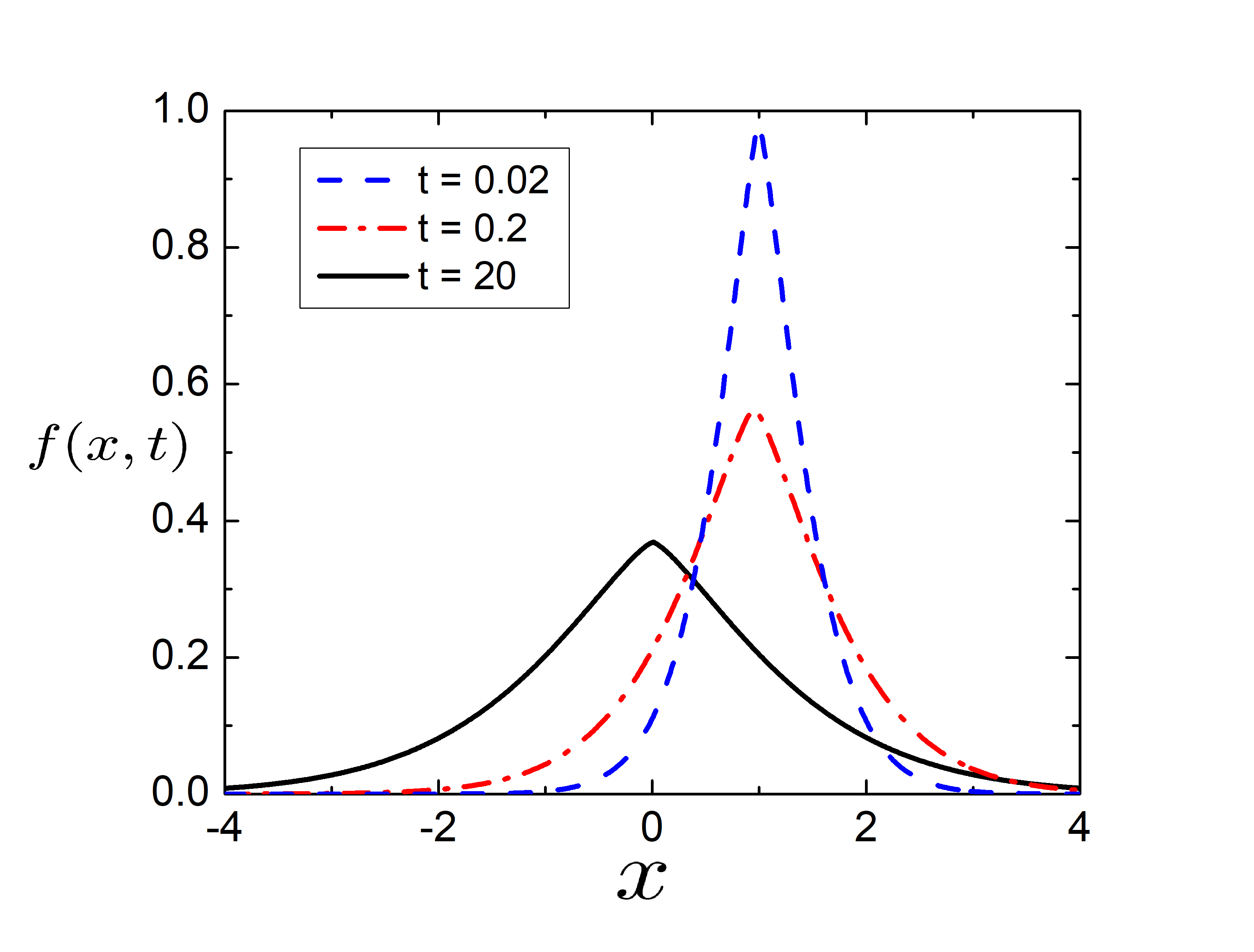
Figure 1: The evolution of PDF (Eq. 16) for $\mu=\frac{4}{3}$, $\nu=4$, $\varkappa=\frac{1}{2}$, $\kappa=\frac{1}{4}$, $x_{0}=1$.

Onsager and Machlup introduced functional representation of the corresponding probability density function [48]

$$f(x,t)=f_{0}\exp\left(-\frac{\psi}{2\varkappa}\right),$$ (6)

or

$$f(x,t)=\sqrt{\frac{\kappa}{2\pi\varkappa(1-e^{-2\kappa t})}}\exp\left\{-\frac{\kappa(x-x_{0}e^{-\kappa t})^{2}}{2{\varkappa}(1-e^{-2\kappa t})}\right\}.$$ (7)

This function describes evolution of the non-equilibrium system to equilibrium or steady state ($t\to\infty$), where the PDF, (7) reduces to

$$f(x)=\sqrt{\frac{\kappa}{2\pi\varkappa}}\exp\left(-\frac{{\kappa}x^{2}}{2{\varkappa}}\right).$$ (8)

Here, $\varkappa$ is the diffusion coefficient. At $\kappa\to 0$ we obtain the second limiting case of (7):

$$f(x,t)=\frac{1}{2\sqrt{\pi\varkappa t}}\exp\left\{-\frac{(x-x_{0})^{2}}{4\varkappa t}\right\}.$$ (9)

The PDF, (7) is solution of the well-known Fokker-Planck equation

$$\frac{\partial f}{\partial t}=\kappa\frac{\partial}{\partial x}(xf)+\varkappa\frac{\partial^{2}f}{\partial x^{2}}\,.$$ (10)

Here, $\kappa$ corresponds to the potential strength. At $\kappa=0$ Eq. (10) reduces to heat (diffusion) equation

$$\frac{\partial f}{\partial t}=\varkappa\frac{\partial^{2}f}{\partial x^{2}}.$$ (11)

The theory of Onsager and Machlup was generalized in [46]. There, we wrote down the Lagrangian in the form

$${\cal L}(\varphi,\dot{\varphi})=\frac{1}{\mu}|\dot{\varphi}+\kappa\varphi|^{\mu},$$ (12)

From the condition $\delta\phi=\int_{0}^{t}\delta{\cal L}\,d\tau=0$ we obtain the Euler-Lagrange Eq.(3), which leads to the second-order equation $(\mu-1)\ddot{\varphi}+(\mu-2)\kappa\dot{\varphi}-\kappa^{2}\varphi=0$. This permits us to derive the generalized Lagrangian ${\cal L}(\tau,t,x)$ and functional minimum $\psi(t,x)$:

$${\cal L}(\tau,t,x)=\frac{(\nu\kappa)^{\mu}e^{\nu\kappa\tau}|x-x_{0}e^{-\kappa t}|^{\mu}}{\mu e^{\nu\kappa t}(1-e^{-\nu\kappa t})^{\mu}}$$ (13)

$$\psi(t,x)=\int_{0}^{t}{\cal L}(\tau,t,x)\,d\tau=\frac{(\nu\kappa)^{\mu-1}|x-x_{0}e^{-\kappa t}|^{\mu}}{\mu(1-e^{-\nu\kappa t})^{\mu-1}}\,.$$

Here, the shape parameters $\nu$ and $\mu$ are related by

$$\frac{1}{\mu}+\frac{1}{\nu}=1\,,\;\>\mu>1\,,\;\>\nu>1\,.$$ (14)

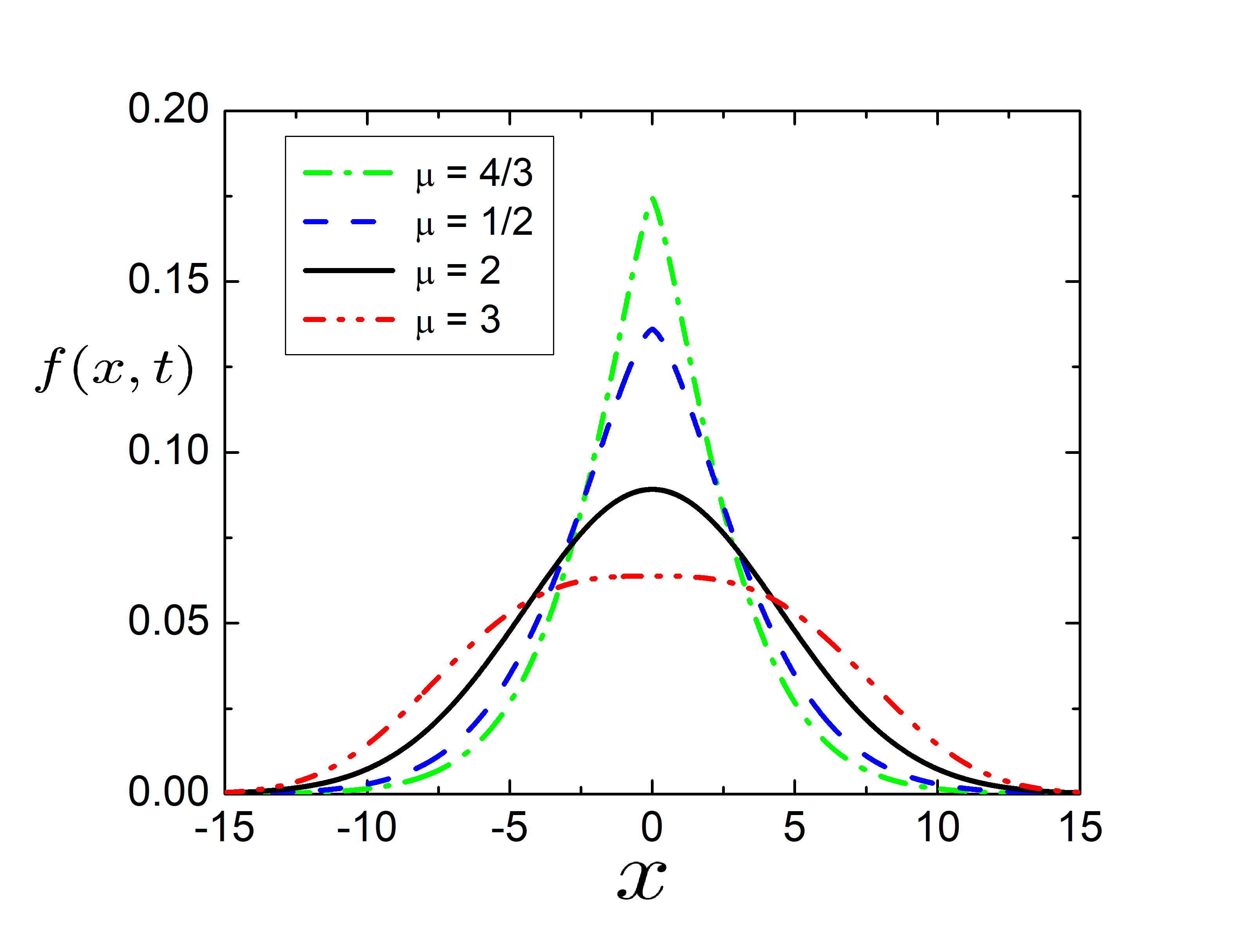
Figure 2: The evolution of PDF (Eq. 23) for $\mu=\frac{4}{3},\frac{3}{2},2,3$, $\varkappa=\frac{1}{2}$.

II.2 Probability density function

We assume the generalized representation of the PDF:

$$f(x,t)=f_{0}\exp\left\{-\frac{\psi}{(\nu\varkappa)^{\mu-1}}\right\}.$$ (15)

Introducing (13) into (15) we get

$$f(x,t)=\frac{\left(\mu\kappa\right)^{\frac{1}{\nu}}}{2\Gamma\left(\frac{1}{\mu}\right)\varkappa^{\frac{1}{\nu}}\left(1-e^{-\nu\kappa t}\right)^{\frac{1}{\nu}}}\times$$

$$\times\exp\left(-\frac{\kappa^{\mu-1}|x-x_{0}e^{-\kappa t}|^{\mu}}{\mu\varkappa^{\mu-1}\left(1-e^{-\nu\kappa t}\right)^{\mu-1}}\right)\,.$$ (16)

This function has the form of the well-studied generalized normal distribution [49]. At $\mu=\nu=2$ we get the case considered in the theory of Onsager and Machlup [48]. The evolution of PDF (16) for these parameter values is plotted at Fig. 1. It roughly resembles the behavior of PDF, described within the fractional derivatives approach [50, 51]. But there are also some discrepancies: the PDF (16) obeys symmetrical shape and has no cusp. Setting $x_{0}=0$ yields

$$f(x,t)=\frac{\left(\mu\kappa\right)^{\frac{1}{\nu}}}{2\Gamma\left(\frac{1}{\mu}\right)\varkappa^{\frac{1}{\nu}}\left(1-e^{-\nu\kappa t}\right)^{\frac{1}{\nu}}}\times$$

$$\times\exp\left(-\frac{\kappa^{\mu-1}|x|^{\mu}}{\mu\varkappa^{\mu-1}\left(1-e^{-\nu\kappa t}\right)^{\mu-1}}\right)\,.$$ (17)

Let us consider discrete form parameters: $\mu=\frac{n+1}{n}$, $\nu=n+1$, $n=1,2,\dots$ and represent time-dependent generalized normal distribution (16) as

$$f(x,t)=\frac{\left(1+\frac{1}{n}\right)^{\frac{1}{n+1}}}{2\Gamma(\frac{n}{n+1})}\left(\frac{\kappa}{\varkappa(1-e^{-(n+1)\kappa t})}\right)^{\frac{1}{n+1}}$$

$$\times\exp\left\{-\left(\frac{\kappa}{\varkappa(1-e^{-(n+1)\kappa t})}\right)^{\frac{1}{n}}\frac{|x|^{1+\frac{1}{n}}}{\mu}\right\}\,.$$ (18)

In this case, the PDF may be considered as the solution of the differential equation

$$\frac{\partial f(x,t)}{\partial t}=\kappa\frac{\partial}{\partial x}(xf(t,x))+(-1)^{n+1}\varkappa\times$$

$$\times\left(\frac{\partial}{\partial x}\frac{a_{1}}{x^{n}}+\dots+\frac{\partial^{n}}{\partial x^{n}}\frac{a_{n}}{x}+\frac{\partial^{n+1}}{\partial x^{n+1}}\right)f(t,x)\,,$$ (19)

at $x\geq 0$.

In the particular case $n=3$, $\mu=\frac{4}{3}$, $\nu=4$ Eq. (19) reduces to the fourth order equation:

$$\frac{\partial f}{\partial t} = \kappa\frac{\partial}{\partial x}\left(xf(x,t)\right)+\varkappa\times$$

$$\times \left(\frac{\partial}{\partial x}\frac{a_{1}}{x^{3}}+\frac{\partial^{2}}{\partial x^{2}}\frac{a_{2}}{x^{2}}+\frac{\partial^{3}}{\partial x^{3}}\frac{a_{3}}{x}+\frac{\partial^{4}}{\partial x^{4}}\right)f(x,t)$$

with

$$a_{1}=-\frac{8}{9}\,;\;\;a_{2}=-\frac{13}{9};\;\;a_{3}=-1\,.$$ (21)

At $t\to\infty$ the PDF (17) tends to the stationary state:

$$f(x,t)=\frac{\left(\mu\kappa\right)^{\frac{1}{\nu}}}{2\Gamma\left(\frac{1}{\mu}\right)\varkappa^{\frac{1}{\nu}}}\exp\left(-\frac{\kappa^{\mu-1}|x|^{\mu}}{\mu\varkappa^{\mu-1}}\right)\,.$$ (22)

At $\kappa\to 0$, corresponding to free motion without confinement, the PDF (17) becomes

$$f(x,t)=\frac{\mu^{\frac{1}{\nu}}}{2\Gamma\left(\frac{1}{\mu}\right)\left(\nu\varkappa t\right)^{\frac{1}{\nu}}}\exp\left(-\frac{|x|^{\mu}}{\mu\left(\nu\varkappa t\right)^{\mu-1}}\right)\,.$$ (23)

The evolution of PDF, given by Eq. (23), is presented at Fig. 2 for different values of the parameter $\mu$. $\mu=2$ corresponds to standard Brownian diffusion, with decreasing of the parameter $\mu$ the distribution becomes more sharp. In the case $\mu=3$ the distribution is more flat as for the Brownian motion.

II.3 Mean-squared displacement

Performing the integration of Eq. (17),

$$\left<x^{2}(t)\right>=\int_{-\infty}^{\infty}x^{2}f(x,t)dx\,,$$ (24)

one gets the mean squared displacement (MSD) [46]

$$\left<x^{2}(t)\right>=\frac{\Gamma\left(\frac{3}{\mu}\right)\mu^{\frac{2}{\mu}}\varkappa^{\frac{2}{\nu}}}{\Gamma\left(\frac{1}{\mu}\right)}\left(\frac{1-e^{-\nu\kappa t}}{\kappa}\right)^{\frac{2}{\nu}}\,.$$ (25)

At $t\to\infty$ the MSD tends to the constant value

$$\left<x^{2}(t)\right>=\frac{\Gamma\left(\frac{3}{\mu}\right)\mu^{\frac{2}{\mu}}\varkappa^{\frac{2}{\nu}}}{\Gamma\left(\frac{1}{\mu}\right)\kappa^{\frac{2}{\nu}}}\,.$$ (26)

In the approximation $\kappa\to 0$ Eq. (25) can be written in the form

$$\left<x^{2}(t)\right>=K_{\alpha}t^{\alpha},$$ (27)

with

$$K_{\alpha} = \frac{\Gamma\left(\frac{3}{\mu}\right)}{\Gamma\left(\frac{1}{\mu}\right)}\mu^{\frac{2}{\mu}}\left(\nu\varkappa\right)^{\frac{2}{\nu}}$$ (28)

$$\alpha = \frac{2}{\nu}=\frac{2\left(\mu-1\right)}{\mu}\,.$$ (29)

In such a way, we obtain the anomalous diffusion processes with non-linear dependence of the MSD on time [50, 51]. The power law constant of the MSD depends on the shape parameters of the generalized normal distribution. At $\mu=2$ again the normal diffusion is obtained:

$$\left<x^{2}(t)\right>=2\varkappa t\,.$$ (30)

II.4 Higher order moments

The fourth moment can be expressed as

$$\left<x^{4}(t)\right>=\int_{-\infty}^{\infty}x^{4}f(x,t)dx\,.$$ (31)

The integration yields

$$\left<x^{4}(t)\right>=\frac{\Gamma\left(\frac{5}{\mu}\right)\mu^{\frac{4}{\mu}}\varkappa^{\frac{4}{\nu}}}{\Gamma\left(\frac{1}{\mu}\right)}\left(\frac{1-e^{-\nu\kappa t}}{\kappa}\right)^{\frac{4}{\nu}}\,.$$ (32)

At $\kappa\to 0$ it becomes

$$\left<x^{4}(t)\right>=\frac{\Gamma\left(\frac{5}{\mu}\right)\mu^{\frac{4}{\mu}}\left(\nu\varkappa\right)^{\frac{4}{\nu}}}{\Gamma\left(\frac{1}{\mu}\right)}t^{\frac{4}{\nu}}\,.$$ (33)

The kurtosis is equal to

$$K=\frac{\left<x^{4}(t)\right>}{\left(\left<x^{2}(t)\right>\right)^{2}}=\frac{\Gamma\left(\frac{5}{\mu}\right)\Gamma\left(\frac{1}{\mu}\right)}{\left(\Gamma\left(\frac{3}{\mu}\right)\right)^{2}}\,.$$ (34)

For $\mu=\frac{4}{3}$ the kurtosis is equal to 4.22, which corresponds to more sharp distribution than a normal distribution.

Odd moments of the symmetrical generalized distribution (17) are equal to zero:

$$\left<x^{2k+1}(t)\right>=0\,,\;\;\text{for}\quad k=0,1,...$$ (35)

The generalized equation for even moments reads:

$$\left<x^{2k}(t)\right>=\int_{-\infty}^{\infty}x^{2k}f(x,t)dx=$$ (36)

$$=\frac{\Gamma\left(\frac{2k+1}{\mu}\right)\mu^{\frac{2k}{\mu}}\varkappa^{\frac{2k}{\nu}}}{\Gamma\left(\frac{1}{\mu}\right)}\left(\frac{1-e^{-\nu\kappa t}}{\kappa}\right)^{\frac{2k}{\nu}},$$ (37)

$$\text{for}\quad k=0,1,...$$

III Resetting

Let us consider the particle returning to the initial position $x=0$ at random times. We denote by $\psi(t)$ the PDF of waiting times between two consecutive resetting events. We consider exponential resetting, corresponding to a Poissonian process:

$$\psi(t)=r{e^{-rt}}$$ (38)

with $r$ being the constant rate of resetting events. The survival probability $\Psi(t)$ is defined as the probability that no resetting event occurs between 0 and $t$,

$$\Psi(t)=1-\int\limits_{0}^{t}{\psi(t^{\prime})dt^{\prime}}={e^{-rt}}\,.$$ (39)

Figure 3: The PDF with resetting for $r=1$, $\mu=\frac{4}{3}$, $\nu=4$, $\varkappa=\frac{1}{2}$ with confinement ($\kappa=\frac{1}{4}$, blue line) and without confinement ($\kappa=0$) at $t=50$. Black dashed line shows PDF calculated according to Eq. (53), while red line corresponds to numerical integration of Eq. (43). In the confinement the distribution becomes more narrow.

III.1 Probability density function under resetting

The probability density to find the particle at location $x$ at time $t$ with rate $r$ is given by

$$p(x,t)=\Psi(t)f(x,t)+\int\limits_{0}^{t}dt^{\prime}r\Psi(t-t^{\prime})f(x,t-t^{\prime})\,.$$ (40)

Here the first term accounts for the realizations where no resetting took place up to the observation time $t$. The second term accounts for the case, when the resetting event occurs at the time $t^{\prime}$, no resetting occurs between $t^{\prime}$ and $t$, and the particle moves freely between these two instants of time. Introducing the survival probability, Eq. (39) into Eq. (40) and using a new variable $\tau=t-t^{\prime}$, we get

$$p(x,t)=e^{-rt}f(x,t)+r\int\limits_{0}^{t}d\tau e^{-r\tau}f(x,\tau)$$ (41)

. The first term may be safely neglected at long times $t\to\infty$

$$p(x,t)=r\int\limits_{0}^{t}d\tau e^{-r\tau}f(x,\tau)\,.$$ (42)

Introducing the PDF, given by Eq. (23) into Eq. (40), we get

$$p(x,t)=\frac{r\mu^{\frac{1}{\nu}}}{2\Gamma\left(\frac{1}{\mu}\right)\left(\nu\varkappa\right)^{\frac{1}{\nu}}}\int_{0}^{t}\tau^{-\frac{1}{\nu}}e^{-\varphi\left(\tau\right)}d\tau$$ (43)

Here we use the function

$$\varphi(\tau)=r\tau+\frac{\tau^{1-\mu}|x|^{\mu}}{\mu\left(\nu\varkappa\right)^{\mu-1}}\,.$$ (44)

Now we find its derivatives

$$\varphi^{\prime}(\tau)=r+\left(1-\mu\right)\frac{\tau^{-\mu}|x|^{\mu}}{\mu\left(\nu\varkappa\right)^{\mu-1}}\,,$$ (45)

$$\varphi^{\prime\prime}(\tau)=\left(\mu-1\right)\frac{\tau^{-\mu-1}|x|^{\mu}}{\left(\nu\varkappa\right)^{\mu-1}}\geq 0\,.$$ (46)

The function $\varphi(\tau)$ attains the minimum at $\tau=\tau_{0}$, which can be found from the condition

$$\varphi^{\prime}(\tau_{0})=0$$ (47)

and equal to

$$\tau_{0}=\frac{|x|}{\nu\varkappa^{\frac{1}{\nu}}r^{\frac{1}{\mu}}}\,.$$ (48)

The extreme value of this function at $\tau=\tau_{0}$ is

$$\varphi(\tau_{0})=\left(\frac{r}{\varkappa}\right)^{\frac{1}{\nu}}|x|\,.$$ (49)

The second derivative of $\varphi(\tau)$ at $\tau=\tau_{0}$ can be calculated as

$$\varphi^{\prime\prime}(\tau_{0})=\frac{\mu\nu r^{1+\frac{1}{\mu}}\varkappa^{\frac{1}{\nu}}}{|x|}\,.$$ (50)

Now let us apply the saddle-point approximation. We perform the Taylor expansion of $\varphi(\tau)$

$$\varphi(\tau)=\varphi\left(\tau_{0}\right)+\frac{1}{2}\left(\tau-\tau_{0}\right)^{2}\varphi^{\prime\prime}(\tau_{0})+...$$ (51)

and introduce it into the PDF (Eq. 43). Let us assume that $1\ll\tau_{0}\ll t$ or

$$|x|\gg\nu\varkappa^{\frac{1}{\nu}}r^{\frac{1}{\mu}}\;;\;\;\;\;t\gg\frac{|x|}{\nu\varkappa^{\frac{1}{\nu}}r^{\frac{1}{\mu}}}\,.$$

In this case the upper and lower integration limits tend to $\pm\infty$ and the PDF can be written as

$$p(x,t)=\frac{r\mu^{\frac{1}{\nu}}}{2\Gamma\left(\frac{1}{\mu}\right)\left(\nu\varkappa\tau_{0}\right)^{\frac{1}{\nu}}}\int_{-\infty}^{\infty}e^{-\varphi(\tau_{0})-\frac{\left(\tau-\tau_{0}\right)^{2}}{2}\varphi^{\prime\prime}(\tau_{0})}d\tau=$$

$$=\frac{\sqrt{2\pi}r\mu^{\frac{1}{\nu}}}{2\Gamma\left(\frac{1}{\mu}\right)\sqrt{\varphi^{\prime\prime}(\tau_{0})}\left(\nu\varkappa\tau_{0}\right)^{\frac{1}{\nu}}}\exp\left(-\varphi\left(\tau_{0}\right)\right)$$ (52)

Introducing Eqs. (49-50) into Eq. (52) we get steady state value of PDF

$$p(x)=\frac{\sqrt{2\pi}r^{\frac{1}{2\nu}}|x|^{\frac{1}{2}-\frac{1}{\nu}}\varkappa^{\frac{1}{\nu^{2}}-\frac{3}{2\nu}}}{2\Gamma\left(\frac{1}{\mu}\right)\nu^{\frac{1}{2}}\mu^{\frac{1}{2}-\frac{1}{\nu}}}\exp\left(-\left(\frac{r}{\varkappa}\right)^{\frac{1}{\nu}}|x|\right).\qquad$$ (53)

This analytical estimation is shown at Fig. 3 as black dashed line. It can be compared with numerical derivation of PDF, obtained by inserting (Eq. 23) into (Eq. 41) and performing numerical integration using Mathematica. The result corresponds to red solid line at Fig. 3. It may be seen that the analytical estimation practically coincide with the result of numerical integration at $t=50$.

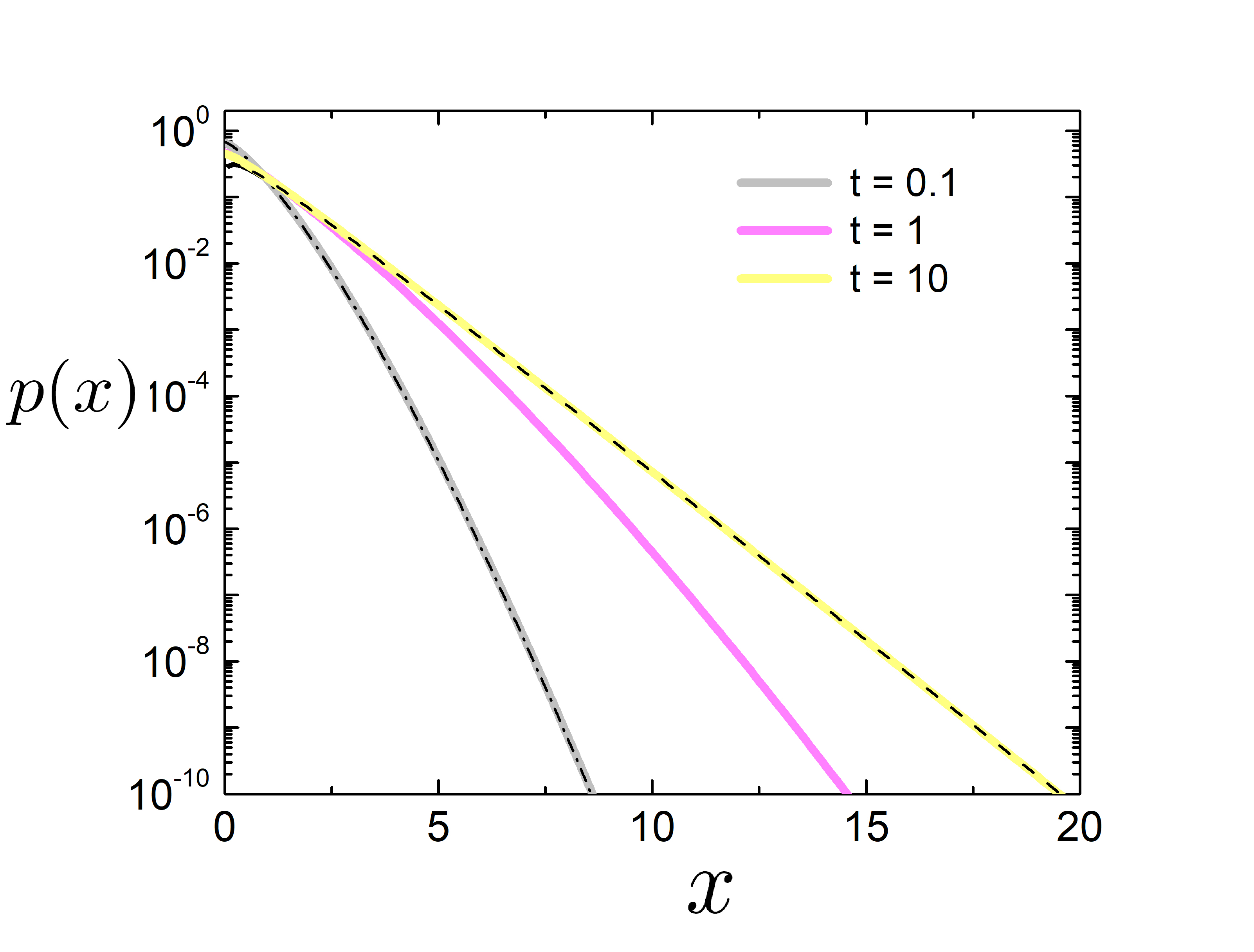
Figure 4: The PDF with resetting for $r=1$, $\mu=\frac{4}{3}$, $\nu=4$, $\varkappa=\frac{1}{2}$, $\kappa=0$ at $t=0.1,\,1,\,10$. Black dashed line shows PDF calculated according to Eq. (53). Black dashed-dotted line depicts PDF free motion without resetting (Eq. 23). Solid yellow, grey and magenta lines corresponds to numerical integration of Eq. (43).

At $t<\tau_{0}$ the minimum is not attained during the observation time. Then the most important impact to the integrand occurs at $\tau\approx t$. In this case the PDF attains the form

$$f(x,t)\sim\left(1+r\right)\frac{\mu^{\frac{1}{\nu}}}{2\Gamma\left(\frac{1}{\mu}\right)\left(\nu\varkappa t\right)^{\frac{1}{\nu}}}\exp\left(-rt-\frac{|x|^{\mu}}{\mu\left(\nu\varkappa t\right)^{\mu-1}}\right)$$ (54)

It corresponds to trajectories, which have undergone no resettings up to time $t$ [18].

The PDF at different time moments is depicted at Fig. 4. At short times the amount of resetting events is negligible, and the PDF is practically the same as without resetting (Eq. 23). At long times it tends to the NESS, given by Eq. (53). At intermediate time the NESS is established in a core region around the resetting center, while outside the core region the system is transient. This phenomena has at first been observed by Majumdar et al. for Brownian motion, fractional Brownian motion and fluctuating interfaces [18].

The PDF for particles in confinement can be obtained numerically by inserting (Eq. 17) into (Eq. 41) and is shown as solid blue line at Fig. 3.

III.2 Mean-squared displacement under resetting

Multiplying Eq. (40) by $x^{2}$ and performing the integration over $x$, we get the equation for the MSD of particles:

$$\left\langle x^{2}(t)\right\rangle=\left\langle x^{2}(t)\right\rangle\Psi(t)+\int_{0}^{t}dt^{\prime}r\Psi(t-t^{\prime})\left\langle x^{2}(t-t^{\prime})\right\rangle\,.$$

(55)

At long times $t\to\infty$ the first term may be neglected and the MSD becomes

$$\left\langle x^{2}(t)\right\rangle=\int_{0}^{t}dt^{\prime}r\Psi(t-t^{\prime})\left\langle x^{2}(t-t^{\prime})\right\rangle\,.$$ (56)

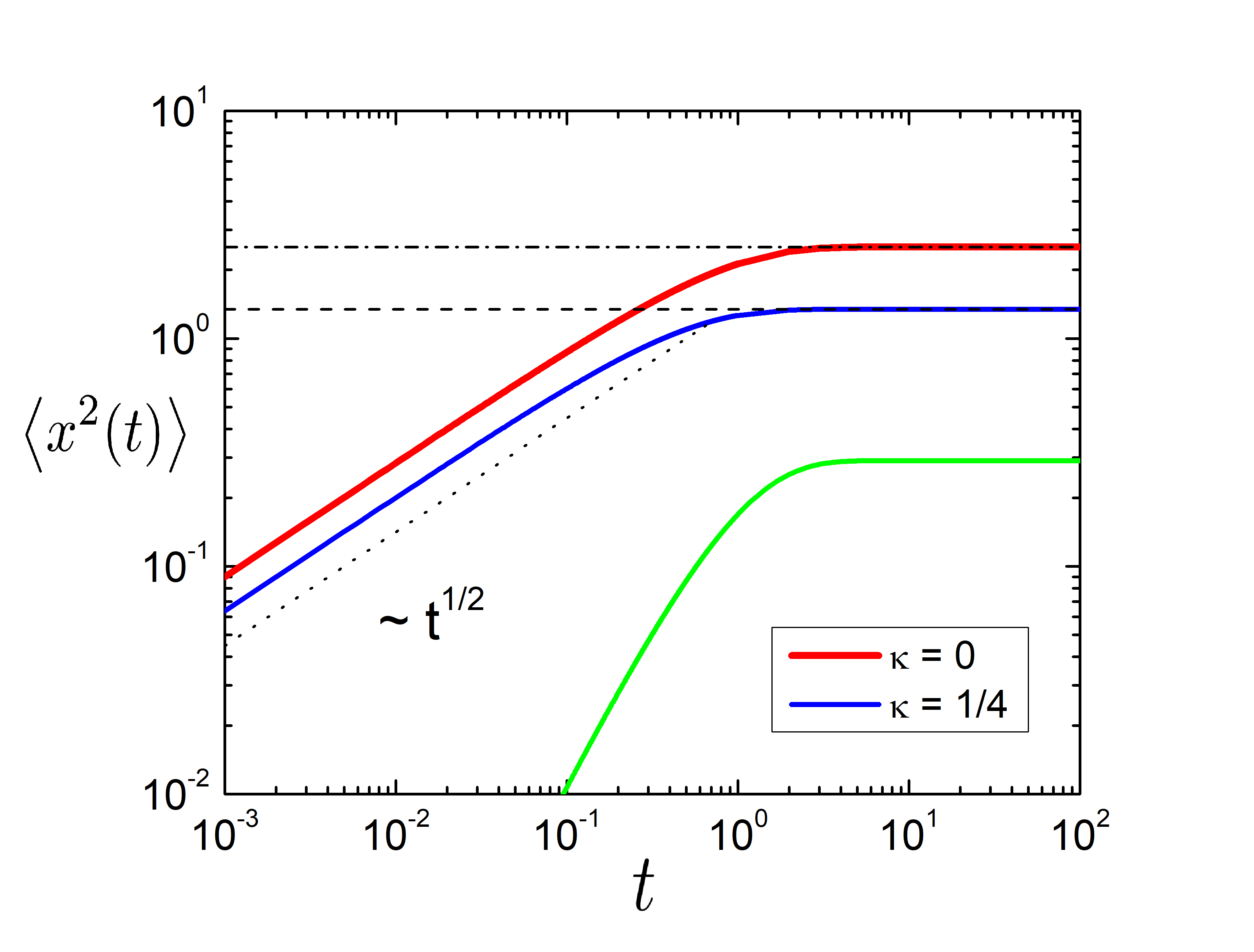
Figure 5: The evolution of MSD with resetting for $r=1$, $\mu=\frac{4}{3}$, $\nu=4$, $\varkappa=\frac{1}{2}$, with and without confinement, $\kappa=\frac{1}{4}$ (Eq. 61) and $\kappa=0$ (Eq. 57), respectively. At short time it evolves according to $\sqrt{t}$ as in the free state. At $t\to\infty$ the MSD tends to the stationary values, given by Eqs. (59) and (64) for $\kappa=0$ (dashed dotted line) and $\kappa=\frac{1}{4}$ (dashed line), respectively.

III.2.1 Free MSD

Introducing Eq. (27) and Eq. (39) into Eq. (55), we obtain

$$\left\langle x^{2}(t)\right\rangle=K_{\alpha}e^{-rt}t^{\alpha}+K_{\alpha}\int_{0}^{t}dt^{\prime}re^{-r(t-t^{\prime})}\left(t-t^{\prime}\right)^{\alpha}$$ (57)

This integral can be calculated numerically, and the result is shown as red line at Fig. 5. Let us now provide some analytical estimations. The integration in the limit $t\to\infty$ yields

$$\left\langle x^{2}(t)\right\rangle=K_{\alpha}r^{-\alpha}\gamma\left(\alpha+1,rt\right)\,.$$

Here $\gamma(a,z)$ is the lower incomplete Gamma function. The MSD rapidly tends to the steady state

$$\left\langle x^{2}(t)\right\rangle_{s}=K_{\alpha}r^{-\alpha}\Gamma\left(\alpha+1\right)\,.$$ (58)

Introducing of Eqs. (28-29) into this expression yields

$$\left\langle x^{2}(t)\right\rangle_{s}=\frac{\Gamma\left(\frac{3}{\mu}\right)}{\Gamma\left(\frac{1}{\mu}\right)}\frac{\mu^{\frac{2}{\mu}}\left(\nu\varkappa\right)^{\frac{2}{\nu}}}{r^{\frac{2}{\nu}}}\Gamma\left(\frac{2}{\nu}+1\right)\,.$$ (59)

This value of stationary MSD is depicted as dashed dotted line at Fig. 5. The case $\mu=2$ corresponds to resetting of standard free Brownian motion, and the MSD attains the value

$$\left\langle x^{2}(t)\right\rangle_{s}=\frac{2\varkappa}{r}\,.$$ (60)

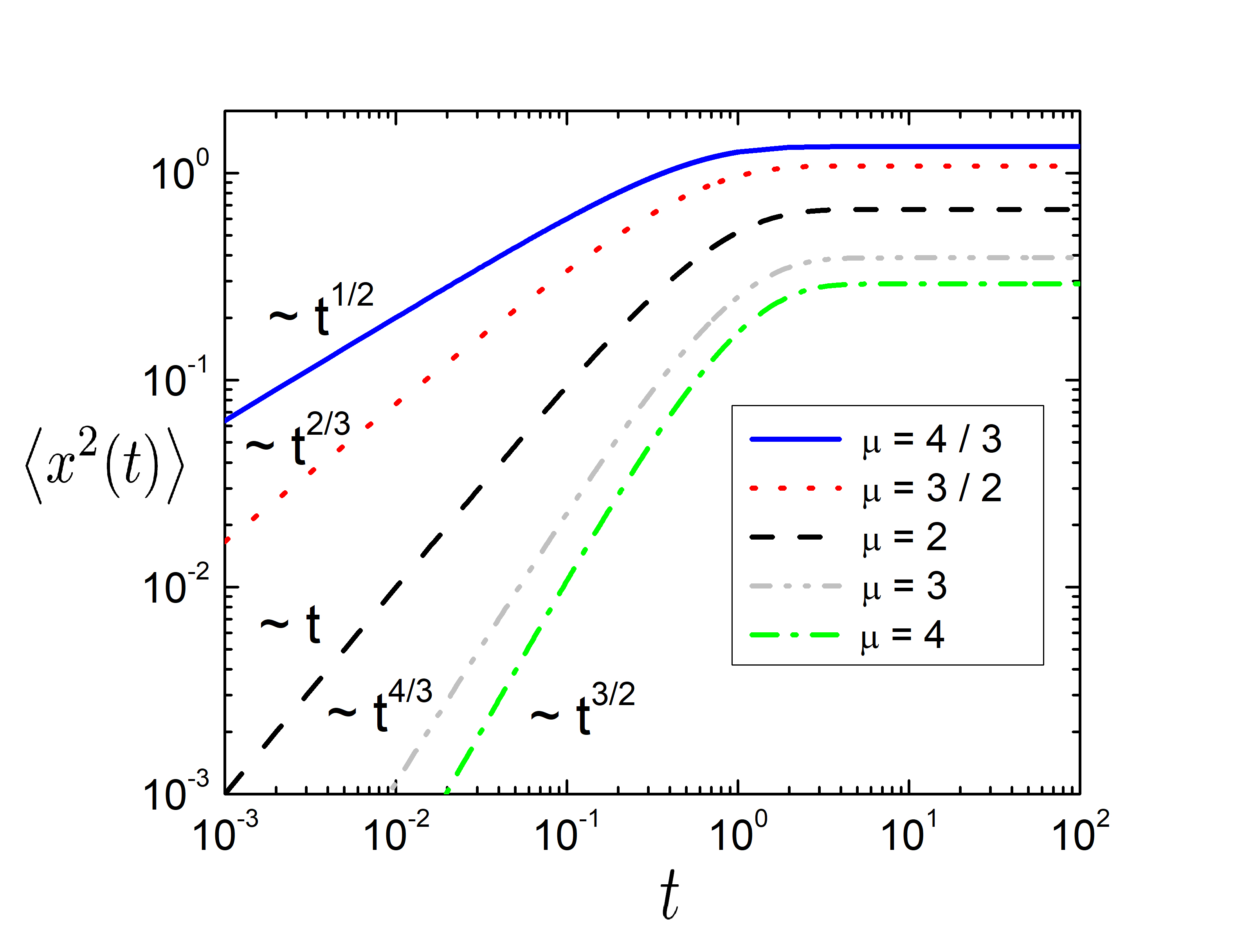
Figure 6: The evolution of MSD with resetting for $r=1$, $\mu=\frac{4}{3},\,\frac{3}{2},\,2,\,3,\,4$, $\varkappa=\frac{1}{2}$, $\kappa=\frac{1}{4}$ (Eq. 61). The time-dependence at short times corresponds to free diffusion without resetting, given by Eqs. (27-29). The case $\mu=2$ corresponds to ordinary Brownian motion in confinement.

III.2.2 MSD in confinement

Introducing Eq. (25) into Eq. (55) leads to

$$\left\langle x^{2}(t)\right\rangle=\frac{\Gamma\left(\frac{3}{\mu}\right)\mu^{\frac{2}{\mu}}\varkappa^{\frac{2}{\nu}}}{\Gamma\left(\frac{1}{\mu}\right)}\left(\frac{1-e^{-\nu\kappa t}}{\kappa}\right)^{\frac{2}{\nu}}e^{-rt}+$$

$$+r\frac{\Gamma\left(\frac{3}{\mu}\right)\mu^{\frac{2}{\mu}}\varkappa^{\frac{2}{\nu}}}{\Gamma\left(\frac{1}{\mu}\right)\kappa^{\frac{2}{\nu}}}\int_{0}^{t}\left(1-e^{-\nu\kappa\tau}\right)^{\frac{2}{\nu}}e^{-r\tau}d\tau\,.$$ (61)

Here $\tau=t-t^{\prime}$. The numerical integration of this expression is given as solid blue line at Fig. 5. Fig. 6 displays the evolution of MSD for values of $\mu$. With increasing of $\mu$ the slope at earlier times becomes more abrupt, the stationary state is obtained earlier and becomes located closer to zero. The behavior of MSD at short times $rt\ll 1$ is the same as motion without resetting, because the amount of resetting event at short times is negligible. The value $\mu=2$ corresponds to resetting of standard Brownian motion in confinement. In this case at short times the MSD has the linear time-dependence.

Let us find the stationary value of MSD. Substituting $\xi=e^{-r\tau}$ into Eq. (61) and neglecting the first term yield

$$\left\langle x^{2}(t)\right\rangle=\frac{\Gamma\left(\frac{3}{\mu}\right)\mu^{\frac{2}{\mu}}\varkappa^{\frac{2}{\nu}}}{\Gamma\left(\frac{1}{\mu}\right)\kappa^{\frac{2}{\nu}}}\int_{e^{-rt}}^{1}d\xi\left(1-\xi^{\frac{\nu\kappa}{r}}\right)^{\frac{2}{\nu}}\,.$$ (62)

In the limit $t\to\infty$ the lower integration limit tends to zero. Using

$$\int_{0}^{1}\left(1-x^{b}\right)^{a}dx=\frac{\Gamma(1+a)\Gamma\left(1+\frac{1}{b}\right)}{\Gamma\left(1+a+\frac{1}{b}\right)}$$ (63)

we obtain

$$\left\langle x^{2}(t)\right\rangle_{s}=\frac{\Gamma\left(\frac{3}{\mu}\right)\mu^{\frac{2}{\mu}}\varkappa^{\frac{2}{\nu}}}{\Gamma\left(\frac{1}{\mu}\right)\kappa^{\frac{2}{\nu}}}\frac{\Gamma\left(1+\frac{2}{\nu}\right)\Gamma\left(1+\frac{r}{\nu\kappa}\right)}{\Gamma\left(1+\frac{2}{\nu}+\frac{r}{\nu\kappa}\right)}\,.$$ (64)

This steady state MSD is depicted as dashed line at Fig. 5. The particle in confinement becomes located closer to the origin compared to the free particle.

For $\mu=2$ the MSD, given by Eq. (64), becomes

$$\left\langle x^{2}(t)\right\rangle_{s}=\frac{\varkappa}{\kappa+\frac{r}{2}}\,.$$ (65)

In this case both presence of external potential and the resetting affect the behavior of MSD in a similar way: the MSD has the same functional dependence on the resetting rate and the potential strength.

IV Conclusion

We have investigated the PDF and MSD of the generalized Ornstein-Uhlenbeck distribution with resetting. Both free diffusive motion and motion in confinement have been considered, while the most studies, concerning resetting, deal with free motion without external potential. The resulting PDF and MSD become stationary in both cases at long times. At first the NESS is established in the core region of the PDF. The MSD increases with increasing of diffusion coefficient and decreases with potential strength and resetting rate. The PDF has exponential dependence on the coordinates and becomes more narrow in the presence of the confinement.

References

- [1] M. R Evans, S. N. Majumdar, and G. Schehr, J. Phys. A 53, 193001 (2020).
- [2] S. Gupta and A. M. Jayannavar, Front. Phys. 10, 789097 (2022).
- [3] A.V. Chechkin, I.M. Sokolov, Phys. Rev. Lett. 121, 050601 (2018).
- [4] A. Pal and S. Reuveni, Phys. Rev. Lett. 118, 030603 (2017).
- [5] A. Pal, Ł. Kuśmierz, S. Reuveni, Phys. Rev. Research 2, 043174 (2020).
- [6] A. Montanari and R. Zecchina, Phys. Rev. Lett. 88, 178701 (2002).
- [7] J. H. Lorenz, PLoS One, 11 043202 (2016).
- [8] S. Reuveni, M. Urbach, and J. Klafter, Proc. Natl. Akad. Sci. U.S.A. 111, 4391 (2014).
- [9] T. Rotbart, S. Reuveni, M. Urbakh, Phys. Rev. E 92, 060101(R) (2015).
- [10] T. Robin, S. Reuveni, M. Urbakh, Nat. Commun. 9, 779 (2018).
- [11] É. Roldán, A. Lisica, D. Sánchez-Taltavull, and S.W. Grill, Phys. Rev. E 93, 062411 (2016).
- [12] D. Boyer, C. Solis-Salas, Phys. Rev. Lett. 112, 240601 (2014).
- [13] D. Noton, L. Stark, Vis Res 11 929 (1971).
- [14] M.P. Eckstein J. Vis. 11 14 (2011).
- [15] W. Cheng and S. Zhang, Journal of Derivatives, 8, 59 (2000)
- [16] S.F. Gray, R.E. Whaley, S.P. Valuing, Journal of Derivatives, 5, 99 (1997)
- [17] M. R. Evans and S. N. Majumdar, Phys. Rev. Lett. 106, 160601 (2011).
- [18] S. N. Majumdar, S. Sabhapandit, G. Schehr Phys. Rev. E 91, 052131 (2015).
- [19] I.M. Sokolov. Phys. Rev. Lett. 130, 067101 (2023).
- [20] A.S. Bodrova, I.M. Sokolov. Phys. Rev. E 101, 062117 (2020).
- [21] M. Montero and J. Villarroel, Phys. Rev. E 87, 012116 (2013).
- [22] V. Méndez and D. Campos, Phys. Rev. E 93, 022106 (2016).
- [23] V.P. Shkilev, Phys. Rev. E 96, 012126 (2017).
- [24] M. Montero, A. Mas-Puigdellósas, J. Villarroel. Eur. Phys. J. B 90, 176 (2017).
- [25] Ł. Kuśmierz, E. Gudowska-Nowak, Phys. Rev. E 99, 052116 (2019).
- [26] L. Kuśmierz, S. N. Majumdar, S. Sabhapandit, and G. Schehr, Phys. Rev. Lett. 113, 220602 (2014).
- [27] L. Kuśmierz, E. Gudowska-Nowak. Phys. Rev. E 92, 052127 (2015).
- [28] T. Zhou, P. Xu, W. Deng. Phys. Rev. Research 2, 013103.
- [29] T. Sandev, V. Domazetoski, L. Kocarev, R. Metzler, and A. Chechkin J. Phys. A: Math. Theor. 55 074003 (2022)
- [30] W. Wang, A.G. Cherstvy, H. Kantz, R. Metzler, and I.M. Sokolov Phys. Rev. E 104 024105 (2021)
- [31] D. Vinod, A.G. Cherstvy, W. Wang, R. Metzler, and I.M. Sokolov, Phys. Rev. E 105 L012106 (2022)
- [32] A.S. Bodrova, A.V. Chechkin, I.M. Sokolov. Phys. Rev. E 100, 012120 (2019).
- [33] A.S. Bodrova, A.V. Chechkin, I.M. Sokolov. Phys. Rev. E 100, 012119 (2019).
- [34] A. P. Riascos, D. Boyer, P. Herringer, and J. L. Mateos, Phys. Rev. E 101 062147 (2020)
- [35] M. Dahlenburg, A. V. Chechkin, R. Schumer, and R. Metzler Phys. Rev. E 103 052123 (2021)
- [36] A.S. Bodrova, I.M. Sokolov. Phys. Rev. E 101, 052130 (2020).
- [37] A.S. Bodrova, I.M. Sokolov. Phys. Rev. E 102, 032129 (2020).
- [38] A. Pal, Ł. Kuśmierz, S. Reuveni, New J. Phys. 21, 113024 (2019).
- [39] A. Pal, Ł. Kuśmierz, S. Reuveni, Phys. Rev. E 100, 040101(R) (2019).
- [40] A. Mas-Puigdellosas, D. Campos, and V. Mendez, Phys. Rev. E 100, 042104 (2019).
- [41] D. Gupta, C.A. Plata, A. Kundu, and A. Pal, J. Phys. A: Math. Theor. 54, 025003 (2020).
- [42] D. Gupta, C.A. Plata, A. Pal, and A. Kundu, J. Stat. Mech., 043202 (2021).
- [43] O. Tal-Friedman, A. Pal, A. Sekhon, S. Reuveni, and Y. Roichman, J. Phys. Chem. Lett. 11, 7350 (2020).
- [44] B. Besga, A. Bovon, A. Petrosyan, S. N. Majumdar, and S. Ciliberto, Phys. Rev. Res. 2, 032029(R) (2020).
- [45] F. Faisant, B. Besga, A. Petrosyan, S. Ciliberto, and S. N. Majumdar, J. Stat. Mech. 2021, 113203 (2021).
- [46] S.I. Serdyukov, Journal of Non-Equilibrium Thermodynamics 48, 243 (2023).
- [47] S.I. Serdyukov, Partial Differ. Equ. Appl. Math. 6, 100453 (2022).
- [48] L. Onsager and S. Machlup, Phys. Rev. 91 1505 (1953).
- [49] S. Nadarajah, J. Appl. Statist. 32, 685 (2005).
- [50] R. Metzler and J. Klafter, Phys. Rep., 339, 1 (2000).
- [51] R. Metzler and J. Klafter, J. Phys. A: Math. Gen., 37, R161 (2004).