PPFL: A Personalized Federated Learning Framework for Heterogeneous Population

Abstract

Personalization aims to characterize individual preferences and is widely applied across many fields. However, conventional personalized methods operate in a centralized manner and potentially expose the raw data when pooling individual information. In this paper, with privacy considerations, we develop a flexible and interpretable personalized framework within the paradigm of federated learning, called PPFL (Population Personalized Federated Learning). By leveraging “canonical models" to capture fundamental characteristics among the heterogeneous population and employing “membership vectors” to reveal clients’ preferences, it models the heterogeneity as clients’ varying preferences for these characteristics and provides substantial insights into client characteristics, which is lacking in existing Personalized Federated Learning (PFL) methods. Furthermore, we explore the relationship between our method and three main branches of PFL methods: clustered FL, multi-task PFL, and decoupling PFL, and demonstrate the advantages of PPFL. To solve PPFL (a non-convex constrained optimization problem), we propose a novel random block coordinate descent algorithm and present the convergence property. We conduct experiments on both pathological and practical datasets, and the results validate the effectiveness of PPFL.

1 Introduction

Personalization is based on customizing models or algorithms to fit individuals’ traits and preferences. It has been extensively considered in various fields such as marketing strategies (Yoganarasimhan, 2020; Smith et al., 2023), precision medicine (Fröhlich et al., 2018; Bonkhoff and Grefkes, 2022), and engineering processes (Lin et al., 2017), to provide differentiated products or services to heterogeneous clients based on the information collected from them.

An intuitive approach to achieve personalization for heterogeneous clients is to estimate the model individually, which requires sufficient data. However, in real-world scenarios, data may be unevenly distributed among clients, with some having a large volume of data while others may have only scarce data. As a result, it is challenging to build an accurate model based on measurements from a single client alone. Hence, conventional personalization methods, like the Mixed-Effect Model (MEM) (Verbeke and Lesaffre, 1996; Bryk and Raudenbush, 1987), Mixture of Experts (MoE) (Feffer et al., 2018), are initiated in a centralized manner, where data are centrally collected, stored, and processed.

However, in most industries, data exist as isolated islands (Zhou and Tang, 2020; Tan et al., 2022). A lack of interconnection between different data owners makes the collection and centralized storage of data time-consuming and expensive. Besides, these data are often deemed sensitive and regarded as a source of confidential and proprietary information (Yang et al., 2020), making data aggregation less feasible in practice. From a legal perspective, enforcing relevant laws and regulations, such as the General Data Protection Regulation (GDPR) in the European Union, sets rules restricting data sharing and storage. Therefore, how to learn personalized models while keeping the training data decentralized (i.e., remaining on the local client device) becomes a crucial problem.

To enable collaborative training of machine learning models among distributed clients without exchanging or centralizing their raw data, a new learning paradigm named Federated Learning (FL) is introduced by McMahan et al. (2017). Instead of transmitting raw data from clients to the central server, in the FL framework, the central server collects the model learned by each client and broadcasts a global model for clients. However, real-world applications are usually faced with a rather heterogeneous population, where each client has diverse underlying patterns (Lin et al., 2017; Yan et al., 2023). Therefore, the distribution of data in different clients can vary greatly, and learning a single global model might result in a significant bias to serve all clients simultaneously (Hanzely et al., 2023). To fill this gap, researchers extensively investigate the incorporation of personalization within the FL framework called personalized federated learning (PFL) and consider it a viable solution for addressing the heterogeneous population challenges in FL (Li et al., 2020; Kairouz et al., 2021). In the typical PFL paradigm, as illustrated in Figure 1, each client maintains a personalized model locally, and the central server orchestras the collaboration amongst clients following the same steps as the vanilla FL: a) At the beginning of each round, the central server broadcasts information (e.g., the global model) for clients to guide their personalized model locally; b) Clients utilize the stored local data and the received information to update their local models; c) Until completing the local update iteration, clients transmit the updated models back to the central server; d) The central server aggregates these updated models to generate the information broadcast in the next round.

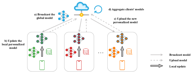
Figure 1: A typical personalized federated learning diagram.

1.1 Related Work

Assuming there are $M$ clients in the system, the vanilla FL approach (McMahan et al., 2017) aims to minimize the weighted sum of each client’s empirical loss:

$$\min_{\theta}\sum_{i=1}^{M}p_{i}f_{i}(\theta),$$

where $f_{i}(\theta)$ represents the empirical loss in the $i$-th client, $\theta$ is the model parameter, and $p_{i}$ corresponds to the importance assigned to the $i$-th client’s loss. To construct personalized models and mitigate the heterogeneous population challenge in FL (Kairouz et al., 2021; Li et al., 2020; Sattler et al., 2020), there are three main streams of the PFL method related to this work.

Clustered FL. Clustered FL is a widely discussed approach that assumes that clients belong to different clusters according to their underlying behavior patterns. Hence, it classifies clients into different clusters and provides personalized models at the group level. The process mainly comprises two primary steps: client identification and personalized model optimization. Client identification aims to find the most suitable cluster for each client. Then, personalized model optimization provides the optimal solution for each cluster. In general, the objective function of clustered FL is given as follows:

$$\min_{\theta_{1},\dots,\theta_{K}}\sum_{k=1}^{K}\sum_{i\in\mathcal{S}_{k}}p_{i}f_{i}(\theta_{k}),$$ (1)

where $\theta_{k}$ represents the personalized model for the $k$-th cluster, and $\mathcal{S}_{k}$ denotes the collection of clients belonging to the $k$-th cluster. In the literature, the client identification step receives more attention. For instance, grouping clients by inspecting the variance of uploaded gradients (Sattler et al., 2020), clustering clients based on the similarity of clients’ feature maps (Liu et al., 2021), and identifying clients by the empirical loss (Ghosh et al., 2020) or the parameter distance (Long et al., 2022). Furthermore, some researchers (Marfoq et al., 2021) propose to classify each local data point instead of each client.

The main superiority of clustered FL is that it explicitly indicates the group information and enhances the interpretability of the population’s heterogeneous behaviors. Although clustered FL can represent the clients’ underlying groups, it ignores the heterogeneity within the group. Due to the complexity of the identification step, the convergence of clustered FL is not guaranteed. Moreover, if all clusters’ models are transmitted to clients for identification, the communication cost is $K$ times that of the vanilla FL. Besides, the separated steps of client identification and personalized model optimization might result in bias and slow the training process.

Multi-task PFL. In this method, clients’ models are trained based on their local datasets, and the server transmits information to clients to guide the development of their personalized models. Consequently, this approach gives rise to the following optimization problem:

$$\min_{\theta_{1},\dots,\theta_{M},{\mathbf{W}}}\sum_{i=1}^{M}p_{i}f_{i}(\theta_{i})+\mathcal{R}(\Theta,{\mathbf{W}}),$$ (2)

where $\theta_{i}$ represents the personalized model in the $i$-th client, $\Theta:=\{\theta_{i}\}_{i=1}^{M}$ denotes the collection of all personalized models, ${\mathbf{W}}$ measures the relationships amongst clients, and $\mathcal{R}$ is a regularization function which plays a crucial role in establishing collaboration mechanisms. For example, T Dinh et al. (2020); Li et al. (2021) employ the $\ell_{2}$ regularization and set ${\mathbf{W}}$ as an identical matrix, $\mathcal{R}(\Theta,{\mathbf{W}}):=\sum_{i=1}^{M}\|\theta_{i}-\theta\|^{2}$, to encourage local personalized models to approach the global model $\theta$ ($\theta:=\sum_{i=1}^{M}p_{i}\theta_{i}$). Besides, the Laplacian regularization, $\mathcal{R}(\Theta,{\mathbf{W}}):=\sum_{i=1}^{M}\sum_{j=1}^{M}w_{ij}\|\theta_{i}-\theta_{j}\|^{2},{\mathbf{W}}=(w_{ij})\in\mathbb{R}^{M\times M}$, is also widely adopted in several works (Smith et al., 2017; Huang et al., 2021; Dinh et al., 2021; Zhang et al., 2021), which promotes pairwise collaboration among clients with similar local distributions.

Although the multi-task PFL is straightforward as it adds regularization to refine the update of local models, the method provides few insights into the heterogeneous behaviors of clients compared with the Clustered FL. Moreover, since inadequate local data will lead to performance degradation (Kamp et al., 2023), the method is less effective when substantial clients have small local datasets.

Decoupling PFL. Decoupling PFL is usually applied to deep models, which generates clients’ private components by partitioning some specific layers from the whole model, and the client-reserved component is intended to specialize in the local distribution. Thus, each client contains both global model parameters and local reserved parameters, and the objective function is represented as follows:

$$\min_{\theta,v_{1},\dots,v_{M}}\sum_{i=1}^{M}p_{i}f_{i}(\theta,v_{i}),$$ (3)

where $v_{i}$ corresponds to the private component in the $i$-th client, and $\theta$ refers to the rest shared model. In the decoupling PFL, researchers propose different strategies for segmenting local private layers and the common global module, such as the local representation module with a global classification layer (Liang et al., 2020), the local head layers with a global representation module (Collins et al., 2021), the local private adapter (Pillutla et al., 2022), and the client-specific embedding layer (Zhang et al., 2023).

Since the personalized component is not engaged in the communication, the decoupling PFL only transmits the rest of the global component and thus takes less communication cost. However, the isolation hinders the post hoc analysis (Murdoch et al., 2019), and the decoupling method also provides less insight into the population. Besides, the lack of collaboration in the personalized component may impair its generalization performance (Xie et al., 2023).

Overall, according to the above discussions, an appropriate PFL framework should probably have the following three properties:

• Its interpretability can reveal clients’ similarities and differences (e.g., clustered FL) for further understanding the underlying patterns of heterogeneous populations.

• Its flexibility can involve standard machine learning models in this framework (e.g., the multi-task PFL for classical personalized models and the decoupling PFL for deep models).

• Its theoretical guarantee can provide an efficient algorithm, at least with a sub-linear convergence rate compared with the multi-task and decoupling PFL under a non-convex optimization setting.

1.2 Contribution

We propose a novel personalized federated learning framework called PPFL (Population Personalized Federated Learning) to achieve the above goals. PPFL is built upon a critical assumption that several underlying mechanisms could represent heterogeneous behavior patterns of populations. Then, the basic idea of PPFL is to use a set of canonical models to represent the heterogeneous population characteristics, and each canonical model corresponds to one mechanism or behavior pattern. It is commonly known that clients may exhibit a mix of those patterns. Thus, we introduce a membership vector ${\mathbf{c}}_{i}=(c_{i1},c_{i2},\dots,c_{iK})^{\top}$ to the $i$-th client, whose element $c_{ik}$ quantifies the degree to which the $k$-th canonical models can represent the $i$-th client’s characteristics. Mathematically, these membership vectors and canonical models can be considered coefficients and a basis system for spanning the modeling space for heterogeneous populations.

Although introducing the membership vectors can bring convenience to building personalized models, it also paves the way for the difficulty of solving PPFL. The reason is that all membership vectors in different clients have a normalization restriction $\sum_{k=1}^{K}c_{ik}=1,\,c_{ik}\geq 0$, which leads to a constrained optimization for PPFL. Solving constrained optimization in a FL framework is a rare setting. Besides, including the additional variable can result in the nonexistence of the convex property (Smith et al., 2017), making it difficult to optimize all variables simultaneously. We also enforce the Laplacian regularization on the membership vectors to facilitate the collaboration between clients with similar data distributions and improve the generalization ability. Additionally, the non-separable Laplacian regularization couples the membership vectors together and impedes the local update of it. To overcome the above hurdles, a federated version of the random block coordinate descent algorithm and its convergence analysis in the non-convex setting are conducted to estimate the membership vectors and canonical models efficiently. Finally, to validate the convergence property and showcase the advantages of our method, we perform experiments on synthetic and real-world datasets, encompassing pathological and practical scenarios.

Our contributions can be summarized as follows:

• Interpretability: The PPFL framework learns the membership vectors and canonical models simultaneously. Compared with the clustered FL methods, PPFL does not need the client identification step, significantly reducing computational complexity. The estimated membership vectors enhance the model-based interpretability. Because it can reveal more of the population’s heterogeneous (within-cluster and between-cluster) behaviors.

• Flexibility: The PPFL framework allows a flexible implementation that can include clustered FL, multi-task PFL, and decoupling PFL (see Section 2.1). Additionally, the proposed method effectively extends the widely used MEM and MoE in the FL setting (see Section 2.2), further demonstrating the proposed model’s versatility.

• Algorithms with Theoretical Guarantees: We propose a novel random block coordinate descent algorithm to solve the constrained non-convex optimization problem of PPFL. The convergence property is provided, and it can achieve the sub-linear $\mathcal{O}(\frac{1}{\sqrt{T}})$ if using full gradient information. To our knowledge, this is the first result of the random block coordinate descent algorithm in the FL framework for the non-convex constrained optimization problem.

The organization of the paper is as follows. In Section 2, we provide the formulation of PPFL, along with implementation details and connections between PPFL and other personalization methods. Section 3 proposes a random block coordinate descent algorithm to solve the PPFL and discusses the convergence property of the proposed algorithm. In Section 4, we evaluate the performance of our approach with other PFL methods on pathological and practical datasets. Section 5 concludes this paper.

2 Population Personalized Federated Learning

This section introduces the formulation of the proposed method, namely PPFL. Then, we investigate the connections between our method and clustered FL, multi-task PFL, and decoupling PFL. Finally, PPFL’s applications with various canonical models demonstrate the framework’s flexibility.

2.1 Formulation of PPFL

We consider a federated learning system with $M$ clients indexed by $i$ and $[M]$ denotes an index set $\{1,2,\dots,M\}$. Assuming there are $K$ distinct behavior patterns among clients, then we introduce the following PPFL framework:

$$\min_{\theta_{\text{com}},\{\theta_{k}\}_{k=1}^{K},\{{\mathbf{c}}_{i}\}_{i=1}^{M}}\quad \sum_{i=1}^{M}p_{i}f_{i}(\theta_{\text{com}},\{\theta_{k}\}_{k=1}^{K},{\mathbf{c}}_{i})+\frac{\lambda}{2}\sum_{i=1}^{M}\sum_{j=1}^{M}w_{ij}\|{\mathbf{c}}_{i}-{\mathbf{c}}_{j}\|^{2},$$ (4)

s.t. $$\mathbf{1}^{\top}{\mathbf{c}}_{i}=1,\;\forall i\in[M],$$ (5)

$${\mathbf{c}}_{i}\geq 0,\;\forall i\in[M],$$ (6)

where $w_{ij}$ is an element of the affinity matrix ${\mathbf{W}}\in\mathbb{R}^{M\times M}$, and $\lambda\geq 0$ serves as a hyperparameter. In Eq.(4), the objective function contains three distinct model parameters: $\theta_{\text{com}}$, $\{\theta_{k}\}_{k=1}^{K}$ and $\{{\mathbf{c}}_{i}\}_{i=1}^{M}$. We will elucidate each of them individually.

• The PPFL framework introduces $K$ canonical models denoted as $\{\theta_{k}\}_{k=1}^{K}$ and expect $\theta_{k}$ to capture inherent characteristics of the $k$-th behavior pattern.

• The PPFL framework utilizes $\theta_{\text{com}}$ to represent the shared global parameter. The shared parameter $\theta_{\text{com}}$ is designed to carry out similar tasks as in the decoupling PFL, such as extracting common representation.

• The PPFL framework employs a $K$-dimension membership vector, ${\mathbf{c}}_{i}=(c_{i1},c_{i2},\dots,c_{iK})^{\top}\in\mathbb{R}^{K}$ assigned to the $i$-th client, whose elements reflect the degree to which canonical models can represent a client. Moreover, considering the interpretability, we require the membership vector ${\mathbf{c}}_{i}$ to fall into a simplex space (see Eq.(5) and (6)).

According to this framework, we can assess the characteristics of each client and derive insights into the heterogeneous population through the membership vector, where the element with a higher value indicates the more significant similarity between the client’s behavior and the corresponding captured characteristics. Meanwhile, based on Chen et al. (2022), canonical models can capture the intrinsic structure and avoid collapse (Chen et al., 2023) in the presence of the underlying cluster structure. Besides, since clients share most parts of the model, PPFL can alleviate the lack of local data and be used in clients with limited local data (Liang et al., 2020). Moreover, since the size of the canonical model is small, the communication cost increases slightly than the linear growth in clustered FL. The application of Laplacian regularization encourages the membership vectors of clients with similar local distributions to be close to each other and captures the intrinsic relationships among clients.

The proposed PPFL allows flexibility in its implementation. As shown in Figure 2a and 2b, using the feature extractor $\theta_{\text{com}}$ as an illustrative example, we present two potential architectures of PPFL. In the first architecture shown in Figure 2a, the output of the $k$-th canonical model is multiplied by $c_{ik}$, and the weighted sum of these outputs is passed into the next layer, i.e., $\sum_{k=1}^{K}{\mathbf{c}}_{ik}r(\theta_{k})$, where $r$ is a function of $\theta_{k}$. Instead of manipulating the outputs, the second architecture in Figure 2b operates on the parameter space, where the personalized model ${\theta}_{i}$ is a linear combination of the canonical models $\{\theta_{k}\}_{k=1}^{K}$ with the weight ${\mathbf{c}}_{i}$, i.e., ${\theta}_{i}=\sum_{k=1}^{K}c_{ik}\theta_{k}$, and the output is generated by $r(\theta_{i})$. With an appropriate value of the hyperparameter $\lambda$ and different architectures, the proposed method is capable of establishing connections with existing PFL methods.

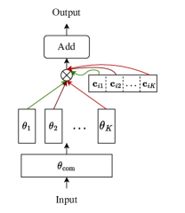
(a)

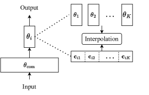
(b)

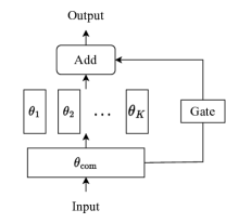
(c)

Figure 2: Two possible structures of PPFL and the structure of MoE. (a) The extracted feature by $\theta_{\text{com}}$ is passed to $K$ parallel canonical models, and the weighted sum of canonical models’ outputs are fed into the next module to give the final prediction; (b) The personalized module is the linear combination of $K$ canonical models with the weight vector $\mathbf{c}_{i}$ and substitutes for the parallel structure to process the extracted feature; (c) The typical MoE structure. The gate module receives the input feature and generates a probability vector to choose which expert to activate.

Connections with clustered FL. With an appropriate model structure, we will show that the clustered FL methods are included in the PPFL framework. Specifically, as shown in Figure 3a, we create a virtual structure by incorporating a replica of $\theta_{\text{com}}$ into each canonical model, and the combination can be considered as the cluster-specific model in clustered FL. If $\lambda=0$ and the max rule (i.e., $\arg\max_{k}c_{ik}$) is further applied to find the best cluster for each client, then the original objective function in (4) becomes as follows:

$$\min_{\{\theta_{k}\}_{k=1}^{K},\{{\mathbf{c}}_{i}\}_{i=1}^{M}}\sum_{k=1}^{K}\sum_{i\in\mathcal{S}_{k}}p_{i}f_{i}(\theta_{k}),$$ (7)

where, with a slight abuse of notation, $\theta_{k}$ represents the combination of the $k$-th canonical model and $\theta_{\text{com}}$, and the set $\mathcal{S}_{k}:=\{i|\arg\max_{k}c_{ik}=k,i\in[M]\}$.

Furthermore, if the constraints on ${\mathbf{c}}_{i}$ are omitted and $c_{ik}$ is directly calculated as the reciprocal of the loss $f_{i}(\theta_{k})$, (i.e., $c_{ik}\propto 1/f_{i}(\theta_{k})$), the above formulation reduces to the basic form of clustered FL (Ghosh et al., 2020). However, with the parameter ${\mathbf{c}}_{i}$, we can parameterize the client identification process and discard the step of similarity calculation in clustered FL, which preserves the continuity of the optimization process and leads to less time for convergence. Meanwhile, the proposed PPFL allows us to capture the within-cluster heterogeneity and customize each client’s model.

Connections with multi-task PFL. With the second architecture in Figure 2b, let the personalized model $\theta_{i}$ in client $i$ comprise $\theta_{\text{com}}$ and the interpolated term $\sum_{k=1}^{K}c_{ik}\theta_{k}$, i.e., $\theta_{i}=[\theta_{\text{com}};\sum_{k=1}^{K}c_{ik}\theta_{k}]$. Plugging $\theta_{i}$ into the objective function in (4) leads to:

$$\min_{\{\theta_{i}\}_{i=1}^{M}} \sum_{i=1}^{M}p_{i}f_{i}(\theta_{i})+\frac{\lambda}{2}\sum_{i=1}^{M}\sum_{j=1}^{M}w_{ij}\|{\mathbf{c}}_{i}-{\mathbf{c}}_{j}\|^{2}.$$ (8)

Compared to the problem (2) with Laplacian regularization, PPFL imposes regularization on ${\mathbf{c}}_{i}$ instead of $\theta_{i}$. Since the values of $\theta_{\text{com}}$ are consistent across clients as well as $\{\theta_{k}\}_{k=1}^{K}$, it is reasonable to conduct the pairwise comparison of the various membership vectors. While, if plugging $\theta_{i}=[\theta_{\text{com}};\sum_{k=1}^{K}c_{ik}\theta_{k}]$ into the objective function (2), we can still derive the similar formulation as (8), which demonstrates the equivalence between these two objective functions. Moreover, instead of a similar objective function, PPFL can alleviate the flaws of multi-task PFL. Since the $K$-dimension vector has a relatively smaller size than $\theta_{i}$, the reduced regularization of PPFL in (8) can alleviate the mismatch problem during the calculation of client similarity (Jeong and Hwang, 2022). Besides, the model parameter-sharing mechanism and the low-dimension client-specific vector in PPFL can reduce the data requirement for local training and mitigate the issue of insufficient local data (Liang et al., 2020).

Connections with decoupling PFL Since both $\theta_{\text{com}}$ and $\{\theta_{k}\}_{k=1}^{K}$ are shared among clients, as depicted in Figure 3b, we can use $\theta$ to represent the collection of them, regardless which architecture is applied. Then, we reformulate the original objective function (4) as:

$$\min_{\theta,\{\mathbf{c}_{i}\}_{i=1}^{M}} \sum_{i=1}^{M}p_{i}f_{i}(\theta,\mathbf{c}_{i})+\frac{\lambda}{2}\sum_{i=1}\sum_{j=1}w_{ij}\|{\mathbf{c}}_{i}-{\mathbf{c}}_{j}\|^{2},$$ (9)

which matches the objective function in the decoupling PFL (3) when $\lambda=0$.

Despite the similar objective function, PPFL and the decoupling PFL are guided by distinct underlying principles. The decoupling PFL emphasizes that the local-reserved module can specialize in the local data distribution without communication. Moreover, by incorporating Laplacian regularization, clients can utilize other clients’ membership vector information, which promotes collaboration among clients and enhances the generalization performance.

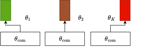
(a)

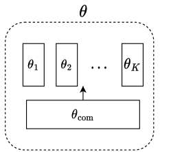
(b)

Figure 3: Virtual structures. (a) The replica of $\theta_{\text{com}}$ and the $k$-th canonical model constitute the $k$-th group-specific model in clustered FL, and any modification to any one of these replicas will be synchronized to others; (b) $\theta_{\text{com}}$ and $\{\theta_{k}\}_{K}$ remain consistent across clients and packed together to serve as the shared global module in the decoupling PFL.

2.2 Implementation of PPFL with Different Canonical Models

In the following paragraphs, we implement the PPFL for two widely used models: Generalized Linear Model (GLM) and the Deep Neural Networks (DNNs). Subsequently, we discuss the connections with some prominent centralized personalized methods specific to these two models, demonstrating our method’s flexibility.

2.2.1 Generalized Linear Model

In the GLM, the response variable $y$ is assumed to follow a specific distribution from the exponential family and related to the feature vector ${\mathbf{x}}\in\mathbb{R}^{d}$ through a link function $g$, and the expectation of $y$ is

$$\mathbb{E}[y]=g^{-1}({\mathbf{x}}^{\top}\mathbf{b}).$$ (10)

Due to the simple formulation of GLM, the parameter $\theta_{\text{com}}$ is dispensable when adopting the PPLF to develop personalized GLM. Following the architectures in Figure 2a and 2b, given the membership vector and $\{\theta_{k}\}_{k=1}^{K}$, we can obtain two potential formulations of the prediction for the $l$-th data point in client $i$ as

$$\hat{y}_{il}=\sum_{k=1}^{K}c_{ik}g^{-1}({\mathbf{x}}_{il}^{\top}\theta_{k}),$$ (11)

and

$$\hat{y}_{il}=g^{-1}({\mathbf{x}}_{il}^{\top}\theta{\mathbf{c}}_{i}),$$ (12)

respectively, where $\theta=[\theta_{1},\theta_{2},\dots,\theta_{K}]\in\mathbb{R}^{d\times K}$ is a stacked matrix of all canonical models.

Specifically, we present the detailed prediction formulas for the standard linear regression and logistic regression as follows:

• Linear Regression: In the linear regression model, the link function $g$ is the identity function. Then, Eq.(11) and (12) lead to the same prediction $\hat{y}_{il}=\sum_{k=1}^{K}c_{ik}{\mathbf{x}}_{il}^{\top}\theta_{k}={\mathbf{x}}^{\top}_{il}\theta{\mathbf{c}}_{i}$ for the $l$-th data point in client $i$.

• Logistic Regression: For a binary classification problem, the link function $g$ is the logit function. In this instance, the predictions $\hat{y}_{il}$ obtained from Eq.(11) and (12) are different, denoted as $\hat{y}_{il}=\sum_{k=1}^{K}c_{ik}\frac{1}{1+\exp(-{\mathbf{x}}_{il}^{\top}\theta_{k})}$ and $\hat{y}_{il}=\frac{1}{1+\exp(-{\mathbf{x}}_{il}^{\top}\theta{\mathbf{c}}_{i})}$ respectively.

Typically, Eq.(11) and (12) yield different outcomes with their own implications. In Eq.(11), the client membership vector ${\mathbf{c}}_{i}$ scores the predictions of these canonical models, and the weighted sum is yielded as the final prediction. In contrast, Eq.(12) first constructs the personalized model spanned by $\{\theta_{k}\}_{k=1}^{K}$ and then plugs it into the formulation of GLM (10).

Through either Eq.(11) or (12), we can apply PPFL to the personalization for GLM. Moreover, PPFL also connects with other personalized GLM variants, such as collaborative learning (Lin et al., 2017; Feng et al., 2020) and the widely used General Linear Mixed Model (GLMM).

For the collaborative method, Lin et al. (2017) propose a collaborative model to deal with the linear regression problem, and the objective function is

$$\min_{\theta,\{{\mathbf{c}}_{i}\}_{i=1}^{M}}\quad \sum_{i=1}^{M}\sum_{l=1}^{n_{i}}\|y_{il}-\mathbf{x}_{il}^{\top}\theta\mathbf{c}_{i}\|_{2}^{2}+\frac{\lambda}{2}\sum_{i,j}w_{ij}\|\mathbf{c}_{i}-\mathbf{c}_{j}\|_{2}^{2},$$ (13)

s.t. $$\mathbf{1}^{\top}{\mathbf{c}}_{i}=1,\;\forall i\in[M],$$

$${\mathbf{c}}_{i}\geq 0,\;\forall i\in[M].$$

Feng et al. (2020) also propose a similar collaborative logistic regression model that has the following objective function

$$\min_{\theta,\{{\mathbf{c}}_{i}\}_{i=1}^{M}}\quad \sum_{i=1}^{M}\sum_{l=1}^{n_{i}}\Big{\{}y_{il}\log(\frac{1}{1+\exp(-\mathbf{x}_{il}^{\top}\theta\mathbf{c}_{i})})+(1-y_{il})\log(\frac{1}{1+\exp(\mathbf{x}_{il}^{\top}\theta\mathbf{c}_{i})})\Big{\}}+$$

$$\quad\frac{\lambda}{2}\sum_{i,j}w_{ij}\|\mathbf{c}_{i}-\mathbf{c}_{j}\|_{2}^{2},$$ (14)

s.t. $$\mathbf{1}^{\top}{\mathbf{c}}_{i}=1,\;\forall i\in[M],$$

$${\mathbf{c}}_{i}\geq 0,\;\forall i\in[M].$$

Compared with the objective function (4), the above two formulations are special cases of proposed PPFL. By utilizing the Eq.(12) while omitting $\theta_{\text{com}}$, we can obtain the same formulations when $f_{i}$ corresponds to the negative log-likelihood of GLM. Besides, instead of the particular regression problems, PPFL extends its method into the more general GLM problem and provides more personalized implementations. Moreover, PPFL is designed in a decentralized manner and can deal with more complicated models by incorporating $\theta_{\text{com}}$. Furthermore, we demonstrate that PPFL can achieve the same objective function as GLMM in Theorem 3, which is provided in Appendix A.2.

2.2.2 Deep Neural Networks

Due to its ability to automatically extract features and deliver impressive performance, DNNs play a pivotal role in multiple industries (Khan and Yairi, 2018; Qi et al., 2023; Gabel and Timoshenko, 2022). Based on the architectures presented in Figure 2a and 2b, it is natural to adopt PPFL to DNNs, and we can use various types of layers/modules as canonical models. In particular, the architecture of MoE (Shazeer et al., 2017), shown in Figure 2c, is similar to the proposed model structure in Figure 2a. The following part will discuss the connection between these two structures.

Notably, both the experts in MoE and the canonical models in PPFL are purposefully designed to specialize in different underlying subgroups among the data. Furthermore, the membership vector ${\mathbf{c}}_{i}$ performs the same function as the weight vector generated by the gating function in MoE (Shazeer et al., 2017). However, the weight vector calculation differs between the MoE model and PPFL, reflecting different cores behind these two methods. In the MoE, the weight vector is calculated from the input data through the gate function to find the best expert for each data point, e.g., $\text{Softmax}(\theta_{g}\mathbf{x})$, where the matrix $\theta_{g}$ is the parameter of the gate function. In contrast, in PPFL, the membership vector is independent of the input data and captures the client’s characteristics. Although the less detailed guide for each data point may reduce the accuracy, PPFL can directly reveal clients’ preferences, enhancing interpretability.

3 Algorithm for PPFL

This section will design an efficient algorithm to solve PPFL and analyze its convergence property.

3.1 Algorithms Design

Adopting the structure in Figure 3b, we use $\theta$ to represent the combination of the shared parameters $\theta_{\text{com}}$ and $\{\theta_{k}\}_{k=1}^{K}$. Let ${\mathbf{C}}=[{\mathbf{c}}_{1}^{\top},\dots,{\mathbf{c}}_{M}^{\top}]^{\top}\in\mathbb{R}^{KM}$ be the concatenated vector of all membership vectors, ${\mathbf{L}}=({\mathbf{D}}-{\mathbf{W}})\otimes{\mathbf{I}}\in\mathbb{R}^{KM\times KM}$ be a Laplacian matrix, $\otimes$ is the Kronecker product, and ${\mathbf{D}}$ be a diagonal matrix with the element $d_{ii}=\sum_{j=1}^{M}w_{ij}$. We reformulate the PPFL framework (4) as

$$\min_{\theta,{\mathbf{C}}} F(\theta,{\mathbf{C}})=\sum_{i=1}^{M}\,p_{i}f_{i}(\theta,{\mathbf{c}}_{i})+\lambda{\mathbf{C}}^{\top}{\mathbf{L}}{\mathbf{C}},$$ (15)

s.t. $${\mathbf{C}}\in\mathcal{C},$$

where the feasible set $\mathcal{C}\subset\mathbb{R}^{KM}$ corresponds to the Cartesian product of $M$ simplex spaces. In the reformulated optimization problem (15), let ${\mathbf{z}}=\{\theta,{\mathbf{C}}\}$ represent the collection of these two model parameters with elements indexed by $h\in\{1,2\}$ (i.e., ${\mathbf{z}}_{1}=\theta$ and ${\mathbf{z}}_{2}={\mathbf{C}}$).

Based on the above reformulation, we can find that designing an FL algorithm to solve (15) has the following three challenges. First, the jointly convex property of $F$ (i.e., $F$ is both convex in $\theta$ and ${\mathbf{C}}$) is a strong condition and hardly guaranteed even for the commonly used basic models (e.g., GLM in Section 2.2). Thus, solving these parameters $\theta$ and ${\mathbf{C}}$ simultaneously is impractical (Smith et al., 2017). Second, the local loss function $f_{i}$ with $i\in[M]$ contains its membership vector ${\mathbf{c}}_{i}$ with a normalization restriction $\sum_{k=1}^{K}c_{ik}=1,c_{ik}\geq 0$, which leads to a constrained optimization in an FL setting. Third, the non-separable Laplacian regularization usually complicates the process since it involves dependency on other membership vectors.

To cope with these issues, we propose a Randomized Block Coordinate Descent (RBCD) algorithm under the FL setting, outlined in Algorithm 1. Instead of updating variables jointly, RBCD-based algorithms decouple variables and optimize only one block of variables by fixing the others (Bertsekas, 1999). Thus, the proposed algorithm can efficiently solve the optimization problem with multiple variables without the jointly convex property (Qin et al., 2013).

Input: the initial state ${\mathbf{z}}^{0}$, the number of canonical models $K$, the number of communication rounds $T$, the number of local steps $E$, the step sizes $\{\eta_{t}\}_{T}$, $\eta_{1,t}=\eta_{t}/E$, $\eta_{2,t}=\eta_{t}$, the Laplacian matrix ${\mathbf{L}}$ with its hyperparameter $\lambda$, the smoothness parameter $L_{1}$ and $L_{2}$ (see Assumption 1), and probabilities $\rho_{h}$ with $\sum_{h}\rho_{h}=1$

Set the initial state ${\mathbf{z}}^{0}$ for each client;

for $t=0,1,\dots,T-1$ do

       The server randomly selects a block ${\mathbf{z}}_{h}^{t}$ with the probability $\rho_{h}$;

       $G({\mathbf{z}}_{h}^{t},\xi)\leftarrow$ Local Gradient$({\mathbf{z}}_{h}^{t},\eta_{h,t})$ based on Algorithm 2;

      The server computes ${\mathbf{z}}_{h}^{t+1}$ based on Eq.(19) or (24);

       The server synchronizes clients with the updated block ${\mathbf{z}}_{h}^{t+1}$;

      

end for

Output: Set $\bar{{\mathbf{z}}}={\mathbf{z}}^{t^{\prime}}$ according to the probability distribution

$$\mathbb{P}(t^{\prime}=t)=\frac{\eta_{t}\min\limits_{h\in\{1,2\}}\rho_{h}(1-\gamma_{h,t}L_{h})}{\sum_{t=1}^{T}\eta_{t}\min_{h=1,2}\rho_{h}(1-\gamma_{h,t}L_{h})},$$ (16)

where $\gamma_{1,t}=4\eta_{t}$ and $\gamma_{2,t}=\frac{\eta_{t}}{2}$.

Algorithm 1 RBCD-based PPFL algorithm.

Besides, since not all variables in our problem are unconstrained, we utilize the mirror descent method to develop a unified optimization framework to deal with them all. More specifically, given ${\mathbf{z}}_{h}^{t}$ in the feasible set $\mathcal{Z}_{h}$, the descent direction $G$, and the distance-generating function $\omega_{h}$, the updated point ${\mathbf{z}}_{h}^{t+1}$ is obtained as follows:

$${\mathbf{z}}_{h}^{t+1}=P_{h}({\mathbf{z}}_{h}^{t},G,\eta)=\mathop{\rm argmin}_{{\mathbf{z}}_{h}\in\mathcal{Z}_{h}}\langle G,{\mathbf{z}}_{h}-{\mathbf{z}}_{h}^{t}\rangle+\frac{1}{\eta}D_{h}({\mathbf{z}}_{h},{\mathbf{z}}_{h}^{t}),$$ (17)

where $D_{h}({\mathbf{z}}_{h},{\mathbf{z}}_{h}^{t})=\omega_{h}({\mathbf{z}}_{h})-\omega_{h}({\mathbf{z}}_{h}^{t})-\langle\nabla\omega_{h}({\mathbf{z}}_{h}^{t}),{\mathbf{z}}_{h}-{\mathbf{z}}_{h}^{t}\rangle$ is the Bregman distance (Bregman, 1967), and $P_{h}$ represents the prox-mapping. Note that the distance-generating function $\omega_{h}$ is required to be $1$-strongly convex for the norm $\|\cdot\|$.

For the first block (i.e., the parameter $\theta$), we employ the $\ell_{2}$ norm as the distance generating function (i.e., $\omega_{1}(\theta)=\frac{1}{2}\|\theta\|_{2}^{2}$). Since the size of the parameter $\theta$ is usually large, considering the communication cost, we require clients to carry out multiple local steps for optimizing $\theta$ before transmitting it to the server. Thus, given the stochastic gradient descent at $\tau$-th local step in the $i$-th client $\nabla_{\theta}f_{i}(\theta_{i,\tau}^{t};{\mathbf{c}}_{i},\xi_{i,\tau}^{t})$, we derive $\theta_{i,\tau+1}^{t}$ as follows:

$$\theta_{i,\tau+1}^{t} =\arg\min_{\theta}\langle\nabla_{\theta}f_{i}(\theta_{i,\tau}^{t};{\mathbf{c}}_{i},\xi_{i,\tau}^{t}),\theta-\theta_{i,\tau}^{t}\rangle+\frac{1}{2\eta_{1,t}}(\|\theta\|_{2}^{2}-\|\theta_{i,\tau}^{t}\|_{2}^{2}-\langle\theta_{i,\tau}^{t},\theta-\theta_{i,\tau}^{t}\rangle),$$ (18)

where ${\mathbf{c}}_{i}$ is fixed and $\xi_{i,\tau}^{t}$ is the data point randomly selected with the uniform distribution from the local dataset in client $i$ at the current step.

With the first-order optimality condition for the unconstrained problem, the Eq.(18) reduces to

$$\theta_{i,\tau+1}^{t}=\theta_{i,\tau}^{t}-\eta_{1,t}\nabla_{\theta}f_{i}(\theta_{i,\tau}^{t};{\mathbf{c}}_{i},\xi_{i,\tau}^{t}),$$

which is the same as the stochastic gradient descent. Hence, updating the parameter based on (18) is equivalent to the local update in the FedAvg method (McMahan et al., 2017). We achieve the $\theta^{t+1}$ as:

$$\theta^{t+1}=P_{1}(\theta^{t},G(\theta^{t},\xi),\eta)=\theta^{t}-\eta_{1,t}\sum_{i=1}^{M}p_{i}\sum_{\tau=0}^{E-1}\nabla_{\theta}f_{i}(\theta_{i,\tau}^{t};{\mathbf{c}}_{i},\xi_{i,\tau}^{t}),$$ (19)

where $G(\theta^{t},\xi^{t})=\sum_{i=1}^{M}p_{i}\sum_{\tau=0}^{E-1}\nabla_{\theta}f_{i}(\theta_{i,\tau}^{t};{\mathbf{c}}_{i},\xi_{i,\tau}^{t})$ is the accumulated stochastic gradient.

For the membership vector ${\mathbf{c}}_{i}$ restricted in the unit simplex region, the entropy function, i.e., $\omega_{2}({\mathbf{c}})={\mathbf{c}}^{\top}\log{\mathbf{c}}$, is usually adopted as the distance-generating function (Beck and Teboulle, 2003). We utilize the Majorization-Minimization (MM) method (Tuck et al., 2019; Sun et al., 2016) to further deal with the non-separable Laplacian regularization. Concretely, since the affinity matrix ${\mathbf{W}}$ is usually positive semi-definite (Nader et al., 2019), at time $t$, an upper bound of the objective function (Ziko et al., 2020) in (15) is given by

$$\sum_{i=1}^{M}p_{i}f_{i}(\theta,{\mathbf{c}}_{i})+\lambda{\mathbf{C}}^{\top}({\mathbf{D}}\otimes{\mathbf{I}}){\mathbf{C}}-\lambda[({\mathbf{C}}^{t})^{\top}({\mathbf{W}}\otimes{\mathbf{I}}){\mathbf{C}}^{t}+2(({\mathbf{W}}\otimes{\mathbf{I}}){\mathbf{C}}^{t})^{\top}({\mathbf{C}}-{\mathbf{C}}^{t})].$$ (20)

Let $S_{t}(\mathbf{C};\theta)$ denote the above surrogate function. Note that given any feasible $\mathbf{C}\in\mathcal{C}$, the surrogate function $S_{t}(\mathbf{C};\theta)\geq F(\mathbf{C};\theta)$ conditioned on $\theta$ and $S_{t}(\mathbf{C}^{t};\theta)=F(\mathbf{C}^{t};\theta)$. Then, let $\Delta^{K}$ denote the unit simplex space, and we can solve each client’s problem in parallel with

$$\min_{{\mathbf{c}}_{i}\in\Delta^{K}}p_{i}f_{i}(\theta,{\mathbf{c}}_{i})+\lambda d_{ii}\langle{\mathbf{c}}_{i},{\mathbf{c}}_{i}\rangle-2\lambda\langle\sum_{j=1}^{M}w_{ij}{\mathbf{c}}_{j}^{t},{\mathbf{c}}_{i}-{\mathbf{c}}_{i}^{t}\rangle.$$

Since the size of the $K$-dimensional vector is relatively small, we conduct only one mirror descent step for ${\mathbf{c}}$ in the above problem, i.e.,

$${\mathbf{c}}_{i}^{t+1}=\arg\min_{{\mathbf{c}}_{i}\in\Delta^{K}}\langle p_{i}\nabla_{{\mathbf{c}}}f_{i}({\mathbf{c}}_{i}^{t};\theta,\xi_{i}^{t})+2\lambda({\mathbf{L}}{\mathbf{C}}^{t})_{i},{\mathbf{c}}_{i}-{\mathbf{c}}_{i}^{t}\rangle+\frac{1}{\eta}D_{2}({\mathbf{c}}_{i},{\mathbf{c}}_{i}^{t}),$$ (21)

where $({\mathbf{L}}{\mathbf{C}}^{t})_{i}=d_{ii}{\mathbf{c}}_{i}^{t}-\sum_{j=1}^{M}w_{ij}{\mathbf{c}}_{j}^{t}$ is a slice of the vector ${\mathbf{L}}{\mathbf{C}}^{t}$ from index $(i-1)*K$ to $i*K-1$. Through the Eq.(21) and the function $\omega_{2}$, we have

$${\mathbf{c}}_{i}^{t+1}={\mathbf{c}}_{i}^{t}\cdot\frac{\exp(-\eta(\nabla_{{\mathbf{c}}}f_{i}({\mathbf{c}}_{i}^{t};\theta,\xi_{i}^{t})+2\lambda({\mathbf{L}}{\mathbf{C}}^{t})_{i}))}{\langle{\mathbf{c}}_{i}^{t},\exp(-\eta(\nabla_{{\mathbf{c}}}f_{i}({\mathbf{c}}_{i}^{t};\theta,\xi_{i}^{t})+2\lambda({\mathbf{L}}{\mathbf{C}}^{t})_{i}))\rangle},$$

where ${\mathbf{c}}_{i}^{t+1}$ is guaranteed to be in the unit simplex $\Delta^{K}$.

Hence, for the vector ${\mathbf{C}}$, we update all membership vectors simultaneously by Eq.(21), i.e.,

$${\mathbf{C}}^{t+1}=\begin{bmatrix}{\mathbf{c}}_{1}^{t+1}\\ \vdots\\ {\mathbf{c}}_{M}^{t+1}\end{bmatrix}=\begin{bmatrix}\mathop{\rm argmin}\limits_{{\mathbf{c}}_{1}\in\Delta^{K}}\langle G_{{\mathbf{c}}_{1}}({\mathbf{C}}^{t},\xi_{1}^{t}),{\mathbf{c}}_{1}-{\mathbf{c}}_{1}^{t}\rangle+\frac{1}{\eta}D_{2}({\mathbf{c}}_{1},{\mathbf{c}}_{1}^{t})\\ \vdots\\ \mathop{\rm argmin}\limits_{{\mathbf{c}}_{M}\in\Delta^{K}}\langle G_{{\mathbf{c}}_{M}}({\mathbf{C}}^{t},\xi_{M}^{t}),{\mathbf{c}}_{M}-{\mathbf{c}}_{M}^{t}\rangle+\frac{1}{\eta}D_{2}({\mathbf{c}}_{M},{\mathbf{c}}_{M}^{t})\end{bmatrix},$$ (22)

with the stochastic gradient $G({\mathbf{C}}^{t},\xi)$,

$$G({\mathbf{C}}^{t},\xi^{t})=\begin{bmatrix}G_{{\mathbf{c}}_{1}}({\mathbf{C}}^{t},\xi_{1}^{t})\\ \vdots\\ G_{{\mathbf{c}}_{M}}({\mathbf{C}}^{t},\xi_{M}^{t})\end{bmatrix}=\begin{bmatrix}p_{1}\nabla_{{\mathbf{c}}}f_{1}({\mathbf{c}}_{1}^{t};\theta,\xi_{1}^{t})\\ \vdots\\ p_{M}\nabla_{{\mathbf{c}}}f_{M}({\mathbf{c}}_{M}^{t};\theta,\xi_{M}^{t})\end{bmatrix}+2\lambda{\mathbf{L}}{\mathbf{C}}^{t}.$$ (23)

Finally, we have ${\mathbf{C}}^{t+1}$ as follows

$${\mathbf{C}}^{t+1}=P_{2}({\mathbf{C}}^{t},G({\mathbf{C}}^{t},\xi),\eta)=\begin{bmatrix}{\mathbf{c}}_{1}^{t}\cdot\exp(-\eta G_{{\mathbf{c}}_{1}}({\mathbf{C}}^{t},\xi_{1}^{t}))/\langle\exp(-\eta G_{{\mathbf{c}}_{1}}({\mathbf{C}}^{t},\xi_{1}^{t})),{\mathbf{c}}_{1}^{t}\rangle\\ \vdots\\ {\mathbf{c}}_{M}^{t}\cdot\exp(-\eta G_{{\mathbf{c}}_{M}}({\mathbf{C}}^{t},\xi_{M}^{t}))/\langle\exp(-\eta G_{{\mathbf{c}}_{M}}({\mathbf{C}}^{t},\xi_{M}^{t})),{\mathbf{c}}_{M}^{t}\rangle\\ \end{bmatrix}.$$ (24)

In summary, in Algorithm 1, at time $t\in[0,T]$, the server randomly picks a block ${\mathbf{z}}_{h}^{t}$ with the probability $\rho_{h}$ and broadcasts it to clients. Then, based on Algorithm 2, clients carry out the corresponding local update process and upload the accumulated gradient to the server. Subsequently, the server updates the selected block with this gradient using Eq.(19) or (24) and then synchronizes it with clients. Finally, the server outputs the value ${\mathbf{z}}^{t^{\prime}}$ from the trajectory $\{{\mathbf{z}}^{t}\}_{t=1}^{T}$ based on the probability in Eq.(16).

Local Gradient$(\theta^{t},\eta_{1,t})$

       for $i=1,2,\dots,M$ do

             Set $\theta_{i,0}^{t}=\theta^{t}$;

             for $\tau=0,\dots,E-1$ do

                   $\theta_{i,\tau+1}^{t}=\theta_{i,\tau}^{t}-\eta_{1,t}\nabla_{\theta}f_{i}(\theta_{i,\tau}^{t};{\mathbf{c}}_{i},\xi_{i,\tau}^{t})$;

                  

             end for

            Upload the local accumulated gradient $\theta_{i,E}^{t}-\theta^{t}$ to the server;

       end for

      

Return: the weighted sum of local accumulated gradients $\sum_{i=1}^{M}p_{i}(\theta_{i,E}^{t}-\theta^{t})$.

Local Gradient$({\mathbf{C}}^{t},\eta_{2,t})$

       for $i=1,2,\dots,M$ do

             Compute the stochastic gradient $p_{i}\nabla_{{\mathbf{c}}}f_{i}({\mathbf{c}}_{i}^{t};\theta,\xi_{i}^{t})$;

             Upload the stochastic gradient $p_{i}\nabla_{{\mathbf{c}}}f_{i}({\mathbf{c}}_{i}^{t};\theta,\xi_{i}^{t})$ to the server;

            

       end for

      The server concatenates the upload gradient as

$$g({\mathbf{C}}^{t})=[p_{1}\nabla_{{\mathbf{c}}}f_{1}({\mathbf{c}}_{1}^{t};\theta,\xi_{1}^{t})^{T},\cdots,p_{M}\nabla_{{\mathbf{c}}}f_{M}({\mathbf{c}}_{M}^{t};\theta,\xi_{M}^{t})^{T}]^{T};$$

Return: $g({\mathbf{C}}^{t})+2\lambda{\mathbf{L}}{\mathbf{C}}^{t}$.

Algorithm 2 The local gradient computation

Remark 1.

Dang and Lan (2015) propose an RBCD algorithm to solve non-convex problems in a centralized manner. In the FL framework, Wu et al. (2021) treat each local model as a block, and Hanzely et al. (2023) investigate an accelerated BCD algorithm for a jointly convex objective function. Compared with the previous study, the proposed algorithm differs from them in FL, designed to deal with non-convex objective functions with constraints. Furthermore, it considers the communication efficiency in the decentralized setting and incorporates the non-separable regularization term, which is more applicable to general problems.

3.2 Convergence Analysis

In this section, we will demonstrate the convergence properties of the proposed algorithm for the framework (15). Throughout the rest of this paper, $\|\cdot\|$ denotes the $\ell_{2}$ norm if not specified.

Without loss of generality, we assume the objective function $F$ is well-bounded by $F^{*}$ and make the following assumptions:

Assumption 1 (Smoothness).

For the $i$-th client, $i\in[M]$, there exists constants $L_{1}$ and $L_{2}$ such that:

• Given any ${\mathbf{c}}_{i}\in\Delta^{K}$, $\|\nabla_{\theta}f_{i}(\theta^{\prime},{\mathbf{c}}_{i})-\nabla_{\theta}f_{i}(\theta,{\mathbf{c}}_{i})\|\leq L_{1}\|\theta^{\prime}-\theta\|$ for any feasible $\theta^{\prime}$ and $\theta$;

• Given any $\theta$, $\|p_{i}\nabla_{{\mathbf{c}}}f_{i}(\theta,{\mathbf{c}}_{i}^{\prime})-p_{i}\nabla_{{\mathbf{c}}}f_{i}(\theta,{\mathbf{c}}_{i})+2\lambda d_{ii}({\mathbf{c}}_{i}^{\prime}-{\mathbf{c}}_{i})-2\lambda w_{ii}({\mathbf{c}}_{i}^{\prime}-{\mathbf{c}}_{i})\|_{\infty}\leq L_{2}\|{\mathbf{c}}_{i}^{\prime}-{\mathbf{c}}_{i}\|_{1}$ for any $\mathbf{c}$, $\mathbf{c}^{\prime}\in\Delta^{K}$.

Assumption 2 (Unbiased Stochastic Gradient $\&$ Bounded Variance).

For any $\tau\in[0,E-1]$, $i\in[M]$, and $t\in[0,T-1]$, we assume that the stochastic gradient estimated at the random data point $\xi_{i,\tau}^{t}$ is unbiased, i.e.,

• $\mathbb{E}_{\xi_{i,\tau}^{t}}[\nabla_{\theta}f_{i}(\theta;{\mathbf{c}}_{i},\xi_{i,\tau}^{t})]=\nabla_{\theta}f_{i}(\theta;{\mathbf{c}}_{i})$, for any given ${\mathbf{c}}_{i}\in\Delta^{K}$ and any feasible $\theta$;

• $\mathbb{E}_{\xi_{i}^{t}}[\nabla_{{\mathbf{c}}}f_{i}({\mathbf{c}}_{i};\theta,\xi_{i}^{t})]=\nabla_{{\mathbf{c}}}f_{i}({\mathbf{c}}_{i};\theta)$, for any given $\theta$ and any ${\mathbf{c}}_{i}\in\Delta^{K}$.

Furthermore, there exist constants $\sigma_{1}^{2}$ and $\sigma_{2}^{2}$ such that

• $\mathbb{E}_{\xi_{i,\tau}^{t}}\|\nabla_{\theta}f_{i}(\theta;{\mathbf{c}}_{i},\xi_{i,\tau}^{t})-\nabla_{\theta}f_{i}(\theta;{\mathbf{c}}_{i})\|^{2}\leq\sigma_{1}^{2}$, for any given ${\mathbf{c}}_{i}\in\Delta^{K}$ and any feasible $\theta$;

• $\mathbb{E}_{\xi_{i}^{t}}\|\nabla_{{\mathbf{c}}}f_{i}({\mathbf{c}}_{i};\theta,\xi_{i}^{t})-\nabla_{{\mathbf{c}}}f_{i}({\mathbf{c}}_{i};\theta)\|^{2}\leq\sigma_{2}^{2}$, for any given $\theta$ and any ${\mathbf{c}}_{i}\in\Delta^{K}$.

Assumption 3 (Bounded Gradient Diversity).

There exists a constant $\delta^{2}$ such that for any given ${\mathbf{C}}\in\mathcal{C}$ and any feasible $\theta$, we have

$$\sum_{i=1}^{M}p_{i}\|\nabla_{\theta}f_{i}(\theta;{\mathbf{c}}_{i})-\nabla_{\theta}F(\theta,{\mathbf{C}})\|^{2}\leq\delta^{2}.$$

Note that Assumptions 1 and 2 are commonly applied in the optimization field. From Assumption 1, we can further infer that the function $F$ is also $L_{1}$-smooth in $\theta$ for any given ${\mathbf{C}}\in\mathcal{C}$, and the surrogate function defined in Eq.(20) is $L_{2}$-smooth in ${\mathbf{C}}$ for any given feasible $\theta$. Assumption 3 is widely accepted in the FL framework (Pillutla et al., 2022) and controls the heterogeneity across clients by ensuring that the client’s gradient $\nabla_{\theta}f_{i}(\theta,{\mathbf{c}}_{i})$ cannot significantly deviate from the weighted gradient $\nabla_{\theta}F(\theta,{\mathbf{C}})$.

For nonconvex optimization problems, the gradient norm is commonly utilized as a convergence criterion, whereby a gradient norm being $0$ implies a stationary point is obtained. Hence, for the unconstrained parameter $\theta$, we use the gradient norm $\|\nabla_{\theta}F(\theta,{\mathbf{C}})\|$ to indicate whether $\theta$ is converged with a fixed ${\mathbf{C}}$. For the constrained parameter, as suggested by Dang and Lan (2015), the distance between the current parameter and the updated one, $\|\mathcal{G}({\mathbf{z}}_{h}^{t},{\mathbf{z}}_{h}^{t+1},\eta)\|=\frac{1}{\eta}\|({\mathbf{z}}^{t}_{h}-{\mathbf{z}}^{t+1}_{h})\|$, is usually utilized instead of the gradient norm. Hence, for the parameter ${\mathbf{C}}\in\mathcal{C}$, we utilize the criterion

$$\|\mathcal{G}({\mathbf{C}}^{t},{\mathbf{C}}^{t+1}_{+},\eta)\|_{1} =\frac{1}{\eta}\|({\mathbf{C}}^{t}-{\mathbf{C}}^{t+1}_{+})\|_{1},$$

where ${\mathbf{C}}_{+}^{t+1}$ is composed by

$${\mathbf{c}}_{i,+}^{t+1}:=\arg\min_{{\mathbf{c}}_{i}\in\Delta^{K}}\langle p_{i}\nabla_{{\mathbf{c}}}f_{i}({\mathbf{c}}_{i}^{t};\theta)+2\lambda({\mathbf{L}}{\mathbf{C}}^{t})_{i},{\mathbf{c}}_{i}-{\mathbf{c}}_{i}^{t}\rangle+\frac{1}{\eta}D_{2}({\mathbf{c}}_{i},{\mathbf{c}}_{i}^{t}),$$ (25)

i.e., the full gradient $\nabla_{{\mathbf{c}}}f_{i}({\mathbf{c}}_{i}^{t};\theta)$ is employed instead of $\nabla_{{\mathbf{c}}}f_{i}({\mathbf{c}}_{i}^{t};\theta,\xi_{i}^{t})$ in Eq.(21). Furthermore, we define

$$G^{t}=\begin{bmatrix}\nabla_{\theta}F(\theta^{t},{\mathbf{C}}^{t})\\ \mathcal{G}({\mathbf{C}}^{t},{\mathbf{C}}^{t+1}_{+},\eta)\end{bmatrix},$$ (26)

and $\|G^{t}\|^{2}=\|\nabla_{\theta}F(\theta^{t},{\mathbf{C}}^{t})\|^{2}+\|\mathcal{G}({\mathbf{C}}^{t},{\mathbf{C}}^{t+1}_{+},\eta)\|_{1}^{2}$ gives the norm at the current point ${\mathbf{z}}^{t}$.

Remark 2.

In Dang and Lan (2015), the smoothness property of the distance generating function $\omega$ is required to ensure the validity of $\|\mathcal{G}({\mathbf{z}}_{h}^{t},{\mathbf{z}}_{h}^{t+1},\eta)\|$. For the distance generating function $\omega_{2}(\mathbf{c}_{i})=\mathbf{c}_{i}^{\top}\log(\mathbf{c}_{i})$ employed for the parameter $\mathbf{c}_{i}$, the smoothness property does not hold if any element $c_{ik}=0$. To remedy this problem and maintain the validity of $\|\mathcal{G}({\mathbf{z}}_{h}^{t},{\mathbf{z}}_{h}^{t+1},\eta)\|$, we add a some constant term such as $10^{-6}$, to prevent any element of $\mathbf{c}_{i}$ becoming $0$.

With the previously stated assumptions and the defined convergence criterion, we now present the convergence properties of Algorithm 1 in Theorem 1. The detailed proof is provided in Appendix A.1.

Theorem 1.

Under Assumptions 1, 2 and 3, if the learning rate $\eta_{t}$ with $t\in[0,T]$ satisfies $\eta_{t}=\min\{\frac{1}{32EL_{1}},\frac{2}{L_{2}}\}$ and $\eta_{t}=E\eta_{1,t}=\eta_{2,t}$, and $\bar{\mathbf{z}}:={\mathbf{z}}^{t^{\prime}}$ with the probability given in (16), then we have

$$\mathbb{E}[\|\bar{G}\|^{2}]\leq\frac{2(F({\mathbf{z}}^{0})-F^{*})+2\rho_{2}(M+1)\sum_{t=0}^{T-1}\eta_{t}\sigma_{2}^{2}+\rho_{1}\sum_{t=0}^{T}\eta_{t}^{2}(\sigma_{1}^{2}+\delta^{2})}{\sum_{t=0}^{T-1}\eta_{t}\min_{h\in\{1,2\}}\rho_{h}(1-\gamma_{h,t}L_{h})},$$ (27)

where $\gamma_{1,t}=4\eta_{t}$, and $\gamma_{2,t}=\frac{\eta_{t}}{2}$.

The numerator in inequality (27) contains two distinct error terms. The first error term $2\rho_{2}(M+1)\sum_{t=0}^{T-1}\eta_{t}\sigma_{2}^{2}$ arises from the sampling error during gradient computation for $\mathbf{c}$, while the second term $\rho_{1}\sum_{t=0}^{T}\eta_{t}^{2}(\sigma_{1}^{2}+\delta^{2})$ incorporates both the sampling error and divergence parameter $\delta^{2}$. In the following Corollary 1, we demonstrate that the convergence property with a constant learning rate.

Corollary 1.

With the same assumptions in Theorem 1, considering the constant learning rate $\eta_{t}=\frac{1}{\sqrt{T}}$, $T\geq\max\{1024E^{2}L_{1}^{2},\frac{L_{2}^{2}}{4}\}$, we obtain that

$$\mathbb{E}[\|\bar{G}\|^{2}]=\mathcal{O}\Big{(}\frac{2(F({\mathbf{z}}^{0})-F^{*})+\rho_{1}(\sigma_{1}^{2}+\delta^{2})}{\sqrt{T}}+2\rho_{2}(M+1)\sigma_{2}^{2}\Big{)}.$$ (28)

From (28), if $\sigma_{2}^{2}=0$, with a constant learning rate $\eta_{t}=\frac{1}{\sqrt{T}}$, Algorithm 1 achieves the $\mathcal{O}(\frac{1}{\sqrt{T}})$ converge rate. To this end, we can calculate the full gradient for $\mathbf{c}$, which avoids the error derived from the random sampling step. Thus, a new communication efficient algorithm, Algorithm 3 (see Appendix B), is proposed, which updates $\mathbf{c}_{i}$ and $\theta$ alternatively and saves some synchronization cost. Employing the same lemmas, we can drive the same sub-linear convergence rate $\mathcal{O}(\frac{1}{\sqrt{T}})$. This can be verified by the following Theorem 2.

Theorem 2.

Under Assumptions 1, 2 and 3, when taking Algorithm 3 and calculating the full gradient for $\mathbf{c}_{i}$, $i\in[M]$, i.e., $\sigma_{2}^{2}=0$, if the learning rate $\eta$ satisfies:

$$\eta=\min\{\frac{1}{16L_{1}},\frac{1}{L_{2}},(\frac{4\Delta_{F}}{\sigma_{1,1}T})^{1/2},(\frac{4\Delta_{F}}{\sigma_{1,2}T})^{1/3}\},$$ (29)

then we have

$$\frac{1}{T}\sum_{t=0}^{T-1}\mathbb{E}[\|G({\mathbf{z}}^{t})\|^{2}]\leq\frac{(4\Delta_{F}\sigma_{1,1})^{1/2}}{\sqrt{T}}+\frac{(16\Delta_{F}^{2}\sigma_{1,2}^{2})^{1/3}}{T^{2/3}}+\frac{4\Delta_{F}}{(16L_{1}+L_{2})T},$$ (30)

where $\|G({\mathbf{z}}^{t})\|^{2}=\|\nabla_{\theta}F(\theta^{t},{\mathbf{C}}^{t+1})\|^{2}+\|\mathcal{G}({\mathbf{z}}^{t},{\mathbf{z}}^{t+1},\eta)\|_{1}^{2}$, $\Delta_{F}=F({\mathbf{z}}^{0})-F^{*}$, $\sigma_{1,1}=4L_{1}\sigma_{1}^{2}$, and $\sigma_{1,2}=128L_{1}^{2}\delta^{2}$.

Remark 3.

Comparing the proposed RBCD-based PFL algorithm and the alternating minimization variant with the state-of-the-art result presented by Pillutla et al. (2022), where they employ the decoupling method and demonstrate the sub-linear rate for an alternating minimization algorithm for the non-convex unconstrained problem, we achieve an equivalent sub-linear convergence rate for the non-convex constrained problem if taking the full gradient for the constrained variable. To the best of our knowledge, it is the first result of this problem in the FL setting.

4 Experiment

In this section, we evaluate the empirical performance of PPFL both on pathological and practical datasets compared with several baselines, including clustered Fl, multi-task PFL, and decoupling PFL methods.

4.1 Pathological Datasets

In the pathological setting, we split all data into several pre-specified groups based on their labels, and the client’s local datasets are generated based on these groups. Then, we demonstrate the effectiveness and interpretability of the proposed method on these manipulated datasets.

4.1.1 Setup.

In this setting, we generate a domain-heterogeneous version of the MNIST (LeCun et al., 1998) and CIFAR-10 (Krizhevsky, 2009) datasets as suggested by Jeong and Hwang (2022). They stimulate the presence of distinct subgroups among the population, where clients are only allowed to hold one kind of group-specific data. Besides, we also create a synthetic dataset according to Marfoq et al. (2021), where the distribution of the client’s local data is a mixture of group-specific distributions.

Concretely, for domain-heterogenous datasets, we randomly divide $10$ labels into $4$ groups in the MNIST dataset (see Figure 4a, and, e.g., the digital numbers “3" and “0”, are in the first group) and $3$ groups in CIFAR-10 dataset. There are 100 and 80 clients in the MNIST dataset and the CIFAR-10 dataset, respectively, and the number of clients is equally distributed across these groups in both datasets (e.g., clients with ID numbers in the top 25$\%$ are assigned to the first group in MNIST dataset). Additionally, based on the predefined segmentation, samples with the corresponding labels are pooled together and then are equally split for clients within this same group. In the synthetic data set, there are $3$ underlying groups, and the local dataset of each client is a mixed distribution of these groups instead of only one source in domain-heterogeneous datasets. (see Figure 4b, the sample proportion of $k$-th group in client $i$ is $\alpha_{ik}$, $\alpha_{ik}>0$, and $\sum_{k=1}^{K}\alpha_{ik}=1$.) For all data sets, we utilize $80\%$ of each local dataset for training and test the performance on the remaining $20\%$. Further details about experiment setup are provided in Appendix C.

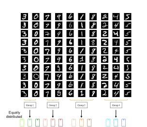
(a) Domain Heterogeneous

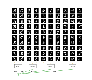
(b) Synthetic

Figure 4: The illustration of the pathological datasets generation process. (a) Digits labels are firstly divided, and samples in each client come from only one group; (b) Digits labels are also categorized, and the sample within each client follows a mixed distribution of these groups.

We implement PPFL with the two proposed structures in Figure 2a and 2b, named PPFL1 and PPFL2, respectively. Then, we consider the purely local training approach and the well-known FedAvg (McMahan et al., 2017) as our baselines. The proposed method is also compared to several multi-task PFL methods, including pFedMe (T Dinh et al., 2020), FedEM (Marfoq et al., 2021), the clustered FL method (Sattler et al., 2020), and the decoupling PFL, FedLG (Liang et al., 2020). Furthermore, we utilize a two-layer perceptron for all methods on the MNIST dataset, MobileNet-v2 (Sandler et al., 2018) for the CIFAR-10 dataset, and a logistic regression model for the synthetic dataset. The code is publicly available.

4.1.2 Performance Evaluation.

For the pathological data sets, all methods’ average test accuracy results over five independent trials are reported as shown in Table 1. We can find that the proposed method achieves the best accuracy on MNIST and CIFAR-10 datasets. Also, it attains comparable accuracy to the best one among baselines on the Synthetic dataset. Note that in the domain-heterogeneous scenario, FedEM, Clustered FL, and PPFL significantly outperform others by taking full advantage of the underlying subgroup structure. However, PPFL has a lower variance than FedEM and clustered FL. This implies our method has stable performance and is less sensitive to the initial parameter value in complicated neural networks. For the synthetic dataset, PPFL has the suboptimal accuracy. Also, the interpolated version of our method is just inferior to FedEM since the latter classifies each data point and thus accords more with the data generation process.

Furthermore, we plot the average accuracy along with the communication round in Figure 5. In domain-heterogeneous datasets, PPFL takes fewer communication rounds to converge than all other methods, implying less communication cost. In the synthetic dataset, PPFL has a similar convergence speed as FedEM. However, we spend less time in each round. As shown in Table 3, FedEM takes more time for local computation, which takes $K$ times as long as the baseline FedAvg method. In contrast, the time consumption of PPFL is slightly increased than FedAvg by taking advantage of the shared parameter $\theta_{\text{com}}$. Based on these two facts, the proposed method can reduce the computation time as well as the communication cost.

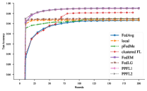
(a) MNIST

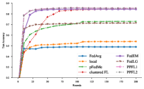
(b) CIFAR-10

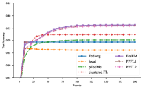
(c) Synthetic

Figure 5: Average Test Accuracy $\&$ Coummunication Cost. The average test accuracy on (a) MNIST dataset, (b) CIFAR-10 dataset, and (c) Synthetic dataset. For (c), FedLG reduces to the FedAvg method and is omitted for clarity.

Table 1: Comparison of PPFL with other methods on pathological datasets. The average test accuracy ($\%$) over five independent trials and the standard deviation ($\%$) are reported.

	Local	FedAvg	pFedMe	FedEM	Clustered FL	FedLG	PPFL1	PPFL2
MNIST	$96.71_{0.05}$	$96.64_{0.05}$	$96.93_{0.06}$	$\bm{99.04}_{0.03}$	$98.19_{0.36}$	$96.95_{0.07}$	$\bm{99.01}_{0.03}$	$99.00_{0.03}$
CIFAR10	$54.10_{1.27}$	$48.98_{0.13}$	$72.96_{0.28}$	$84.93_{2.48}$	$84.73_{0.58}$	$71.30_{1.31}$	$\bm{85.33}_{0.29}$	$85.29_{0.16}$
Synthetic	$66.13_{0.08}$	$69.34_{0.00}$	$70.21_{0.02}$	$\bm{76.25}_{0.73}$	$72.32_{0.29}$	$69.34_{0.00}$	$75.91_{0.59}$	$75.91_{0.59}$

To demonstrate the interpretability of the proposed method, we analyze the values of the matrix ${\mathbf{C}}\in\mathbb{R}^{M\times K}$ (i.e., ${\mathbf{C}}:=[{\mathbf{c}}_{1},\dots,{\mathbf{c}}_{m}]^{\top}$) throughout the training process. This enables us to evaluate its effectiveness in identifying each client’s subgroup and capturing the dataset’s underlying structure. As shown in Figure 6, we present the heatmap of matrix ${\mathbf{C}}$ during the training process on the MNIST dataset. Initially, all elements of ${\mathbf{C}}$ are set to $0.25$. After $20$ communication rounds, our method approximately recognizes the subgroup of each client. Then, the membership vector converges to a unit vector along with the increase of communication rounds. Furthermore, clients within the same group have similar membership vectors, and the directions of membership vectors of clients from different groups are disparate. This result implies the one-to-one correspondence between canonical models and subgroups, and canonical models can specialize in learning the characteristics of each subgroup. In summary, this highlights the proposed method’s effectiveness in capturing clients’ characteristics. The phenomenon in which membership vectors gradually approximate to the underlying structure also exists both on CIFAR-10 and synthetic datasets (see Figure 9 and 11 in Appendix C.5). Thus, with these membership vectors on hand, we can effectively infer the characteristics of subgroups and clients, which can further support business decisions such as the market segmentation strategy.

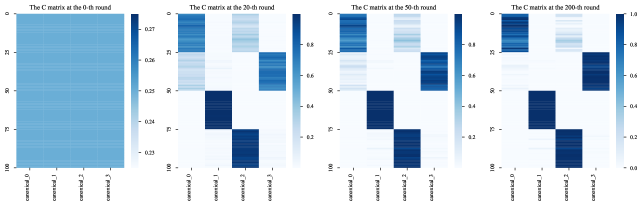
Figure 6: Heatmaps of the matrix ${\mathbf{C}}$ during training on the MNIST dataset. Each row of the matrix denotes the vector ${\mathbf{c}}_{i}$ for a specific client. Darker-colored elements have values closed to $1$.

4.1.3 Effect of the number of canonical models.

In practice, the number of underlying groups among the population is usually unknown. Thus, we examine the influence of the number of canonical models on the group identification performance for clients. Specifically, we vary the value of $N$ on the MNIST data set whose ground-truth number of underlying groups is $4$ and investigate the heatmaps of the final ${\mathbf{C}}$ matrices. As represented in Figure 7, when $N<K$, for example, when $N=3$, clients from different groups employ the same canonical model. When $N\geq K$, canonical models used by clients from different groups are distinct from each other, the complete results on other datasets can be found in the Appendix.

Furthermore, we also investigate the impact of $N$ on the average accuracy. As illustrated in Figure 8, we plot the average accuracy along with $N$ on the synthetic dataset, where the ground-truth number of the underlying group is $3$. We find that when $N<K$, increasing the number of canonical models leads to an improvement in accuracy. However, when $N\geq K$, further increasing $N$ does not guarantee a continuous improvement in accuracy.

In conclusion, when the ground-truth number of underlying groups is unknown, the above results imply that we can use a relatively large number of canonical models to obtain acceptable performance and give us some clues to infer the value of $K$.

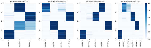
Figure 7: Heatmaps of the final ${\mathbf{C}}$ matrix for different values of $N$ on the MNIST dataset. The assignment of subgroups to specific canonical models varies randomly with different values of $N$. For instance, the first canonical model for $N=3$ may learn a distinct subgroup that differs from its assignment when $N=4$.

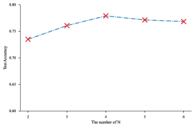
Figure 8: Average test accuracy across different values of $N$ on the Synthetic dataset.

4.2 Practical datasets

Different from pathological settings, in practical scenarios, the clients’ local data are generated by themselves, such as the content of their posts on the Internet. Thus, we conduct experiments on several practical datasets to verify the effectiveness of the proposed method on real-world applications.

4.2.1 Setup

Here, we use two practical datasets: Federated EMNIST (Caldas et al., 2018) and StackOverflow, which focus on character recognition and next-word prediction tasks, respectively. In both datasets, the ground-truth number of underlying groups among the population is unknown, and the size of the local dataset varies across clients. The Federated EMNIST dataset contains 1114 clients, and clients’ local datasets are composed of characters written by themselves. The StackOverflow dataset comprises the textual information of clients’ questions and answers. For this dataset, we select the same 1000 clients as in Pillutla et al. (2022) and the top 10000 most frequent words used by them. For both datasets, $80\%$ of the local data serves as the training set, and the rest is utilized to evaluate model performance.

We utilize the ResNet-18 (He et al., 2016) for the EMNIST dataset and a 4-layer transformer for the StackOverflow dataset. Besides, we adopt local fine-tuning as a baseline alongside FedAvg. In this experiment, clustered FL and FedEM are not considered since they require a substantial amount of graphics memory and are unacceptable in practice. Additionally, we compare our method with the following approaches: 1) Ditto (Li et al., 2021), a multi-task PFL method using the $\ell_{2}$ penalty; 2) pFedMe (T Dinh et al., 2020), a multi-task PFL method using Moreau Envelope; 3) Partial FL (Pillutla et al., 2022) which is a decoupling method. We adopt the same training process as Pillutla et al. (2022) and select the number of canonical models $N$ from an arbitrary set $\{2,5,10,30\}$. Detailed information about experiment setup is provided in Appendix C.

4.2.2 Performance

Table 2 presents the accuracy of all PFL methods over five independent trials. Specifically, on the EMNIST dataset, PPFL achieves the best accuracy over all other methods, demonstrating the proposed method’s effectiveness in practical recognition tasks. While on the StackOverflow dataset, PPFL exhibits lower predictive accuracy than others. The inferior performance may be caused by two reasons: 1) As shown in (Chen et al., 2022), the absence of the underlying fundamental properties(group structure) in this dataset results in a worse performance than the baselines; 2) the other possible reason is the improper structure and the limited number of the canonical model: In the next-word prediction task, suggested by Pillutla et al. (2022), we employ the output layer as the canonical model, which contains about $10^{6}$ parameters. With the limitation of graphics memory, the large number of parameters restricts the number of canonical models (usually at most $50$ in practice). Hence, using a much smaller number of canonical models to represent the large parameter space may lead to deteriorated performance.

Table 2: Comparison of PPFL with other methods on practical datasets. The average test accuracy ($\%$) over five trials and the standard deviation ($\%$) are reported.

	FedAvg	Fintune	Ditto	pFedMe	Partial FL	PPFL1	PPFL2
EMNIST	$93.16$	$94.14_{0.06}$	$94.13_{0.06}$	$94.14_{0.06}$	$94.07_{0.05}$	$\bm{94.19}_{0.02}$	$94.16_{0.02}$
StackOverflow	$23.78$	$25.15_{0.06}$	$\bm{25.16}_{0.06}$	$25.08_{0.06}$	$25.06_{0.03}$	$23.31_{0.01}$	$23.50_{0.01}$

5 Conclusion

This paper presents a novel PFL framework, PPFL, which provides model-based interpretability over existing PFL methods. Assuming the existence of intrinsic characteristics within the heterogeneous population, we contend that the diverse clients cause the heterogeneity exhibited preferences of these characteristics. The proposed method is designed to capture them by canonical models and membership vectors, respectively, which can directly reveal each client’s underlying characteristics and aid in understanding the population. Apart from the interpretability, the flexibility of PPFL enables it to leverage the advantages of existing PFL methods and address their respective limitations. The presented algorithm can handle the constrained problem with non-separable regularization, and the convergence is guaranteed in the non-convex setting. The results in the pathological datasets validate the interpretability and stability of our model, and we also demonstrate comparable accuracy performance in the practical setting, where the underlying characteristics are unknown.

However, as shown in our experiments, if there are no underlying structures in the dataset, the prediction accuracy of our method decreases. Meanwhile, the structures of the backbone model and canonical model should be carefully designed to effectively extract the representation and specialize in disparate underlying characteristics. Besides, the given algorithm requires a full participant, which may cause a high communication cost when dealing with a large number of clients. The algorithm with partial participant and multiple local update steps for all blocks and the corresponding convergence property should be considered in future work.

Supplementary Material to PPFL: A Personalized Federated Learning Framework for Heterogeneous Population

Appendix A Proof of the Theorems

A.1 Proof of the Theorem 1

Let $\Delta_{{\mathbf{z}}_{h}}^{t}(F)=F({\mathbf{z}}_{h}^{t+1},{\mathbf{z}}_{\setminus,h}^{t})-F({\mathbf{z}}_{h}^{t},{\mathbf{z}}_{\setminus,h}^{t})$ denote the loss decrease resulting from the update of block $h$, where ${\mathbf{z}}_{\setminus,h}^{t}$ denotes all other blocks at time $t$ except for the $h$-th block ${\mathbf{z}}_{h}$. The proof is derived as follows: First, we derive an upper bound on $\Delta_{{\mathbf{z}}_{h}}^{t}(F)$ for each block. Next, we take the expectation w.r.t. to the block selection process to induce the overall convergence properties of Algorithm 1. Before presenting the proof of Theorem 1, we will delineate how to obtain upper bounds on $\Delta_{\theta}^{t}(F)$ and $\Delta_{{\mathbf{C}}}^{t}(F)$ respectively in the following lemmas.

Lemma 1.

Holding Assumption 1 $\sim$ 3, for any ${\mathbf{C}}\in\mathcal{C}$, if $\eta_{1,t}\leq\frac{1}{2EL_{1}}$, $0\leq t\leq T$, we have

$$\mathbb{E}_{\xi^{t}}[\Delta_{\theta}^{t}(F)] \leq-\frac{E\eta_{1,t}}{2}(1-2E\eta_{1,t}L_{1}-64E^{2}\eta_{1,t}^{2}L_{1}^{2})\|\nabla_{\theta}F(\theta^{t},C^{t})\|^{2}+32E^{3}\eta_{1,t}^{3}L_{1}^{2}\delta^{2}+$$

$$\quad(8E\eta_{1,t}L_{1}+\frac{1}{2})E^{2}\eta_{1,t}^{2}L_{1}\sigma_{1}^{2}.$$

Proof.

Proof of Lemma 1 Let $G(\theta^{t})=\sum_{i=1}^{M}p_{i}\sum_{\tau=0}^{E-1}\nabla_{\theta}f_{i}(\theta^{t}_{i,\tau};{\mathbf{c}}_{i}^{t})$. According to Assumption 1, we have

$$\Delta_{\theta}^{t}(F) \leq\langle\nabla_{\theta}F(\theta^{t},{\mathbf{C}}^{t}),\theta^{t+1}-\theta^{t}\rangle+\frac{L_{1}}{2}\|\theta^{t+1}-\theta^{t}\|^{2}$$

$$=-\eta_{1,t}\langle\nabla_{\theta}F(\theta^{t},{\mathbf{C}}^{t}),G(\theta^{t})\rangle+\frac{L_{1}}{2}\|\theta^{t+1}-\theta^{t}\|^{2}-\eta_{1,t}\langle\nabla_{\theta}F(\theta^{t},{\mathbf{C}}^{t}),G(\theta^{t},\xi^{t})-G(\theta^{t})\rangle$$

$$=-\eta_{1,t}\langle\nabla_{\theta}F(\theta^{t},{\mathbf{C}}^{t}),\sum_{i=1}^{M}p_{i}\sum_{\tau=0}^{E-1}\nabla_{\theta}f_{i}(\theta_{i,\tau}^{t};{\mathbf{c}}_{i}^{t})-\nabla_{\theta}f_{i}(\theta^{t};{\mathbf{c}}_{i}^{t})+\nabla_{\theta}f_{i}(\theta^{t};{\mathbf{c}}_{i}^{t})\rangle+A_{1}+A_{2}$$

$$=-E\eta_{1,t}\|\nabla_{\theta}F(\theta^{t},{\mathbf{C}}^{t})\|^{2}-\eta_{1,t}\langle\nabla_{\theta}F(\theta^{t},{\mathbf{C}}^{t}),\sum_{i=1}^{M}p_{i}\sum_{\tau=0}^{E-1}\nabla_{\theta}f_{i}(\theta_{i,\tau}^{t};{\mathbf{c}}_{i}^{t})-\nabla_{\theta}f_{i}(\theta^{t};{\mathbf{c}}_{i}^{t})\rangle+A_{1}+A_{2}$$

$$\overset{(a)}{\leq}-\frac{E\eta_{1,t}}{2}\|\nabla_{\theta}F(\theta^{t},{\mathbf{C}}^{t})\|^{2}+\frac{\eta_{1,t}}{2E}\|\sum_{i=1}^{M}p_{i}\sum_{\tau=0}^{E-1}\nabla_{\theta}f_{i}(\theta_{i,\tau}^{t};{\mathbf{c}}_{i}^{t})-\nabla_{\theta}f_{i}(\theta^{t};{\mathbf{c}}_{i}^{t})\|^{2}+A_{1}+A_{2}$$

$$\leq-\frac{E\eta_{1,t}}{2}\|\nabla_{\theta}F(\theta^{t},{\mathbf{C}}^{t})\|^{2}+\frac{\eta_{1,t}}{2E}\sum_{i=1}^{M}p_{i}\|\sum_{\tau=0}^{E-1}\nabla_{\theta}f_{i}(\theta_{i,\tau}^{t};{\mathbf{c}}_{i}^{t})-\nabla_{\theta}f_{i}(\theta^{t};{\mathbf{c}}_{i}^{t})\|^{2}+A_{1}+A_{2}$$

$$\leq-\frac{E\eta_{1,t}}{2}\|\nabla_{\theta}F(\theta^{t},{\mathbf{C}}^{t})\|^{2}+\frac{L_{1}^{2}\eta_{1,t}}{2}\sum_{i=1}^{M}p_{i}\sum_{\tau=0}^{E-1}\|\theta_{i,\tau}^{t}-\theta^{t}\|^{2}+A_{1}+A_{2},$$ (31)

where we utilize $-ab\leq\frac{E}{2}a^{2}+\frac{1}{2E}b^{2}$ in the inequality $(a)$, employ the Jensen’s inequality and convexity property of the $\ell_{2}$ norm in the third inequality, and

$$A_{1} :=\frac{L_{1}}{2}\|\theta^{t+1}-\theta^{t}\|^{2},$$

$$A_{2} :=-\eta_{1,t}\langle\nabla_{\theta}F(\theta^{t},{\mathbf{C}}^{t}),G(\theta^{t},\xi^{t})-G(\theta^{t})\rangle.$$

Let $\xi_{i,[\tau]}^{t}=\{\xi_{i,0}^{t},\dots,\xi_{i,\tau}^{t}\}$ and $\xi_{[\tau]}^{t}=\{\xi_{i,[\tau]}^{t}\}_{M}$. Since

$$\mathbb{E}_{\xi^{t}}[G(\theta^{t},\xi^{t})-G(\theta^{t})] =\sum_{\tau=0}^{E-1}\mathbb{E}_{\xi_{[\tau-1]}^{t}}\left[\mathbb{E}_{\xi_{\tau}^{t}}\left[\sum_{i=1}^{M}p_{i}\nabla_{\theta}f_{i}(\theta^{t}_{i,\tau};{\mathbf{c}}_{i}^{t},\xi_{i,\tau}^{t})-p_{i}\nabla_{\theta}f_{i}(\theta^{t}_{i,\tau};{\mathbf{c}}_{i}^{t})|\xi_{[\tau-1]}^{t}\right]\right]$$

$$=0,$$

and $\nabla_{\theta}F(\theta^{t},{\mathbf{C}}^{t})$ is independent on $\xi^{t}$, taking the expectation w.r.t. $\xi_{t}$ on both sides in (31), we obtain

$$\mathbb{E}_{\xi^{t}}[\Delta_{\theta}^{t}(F)]\leq-\frac{E\eta_{1,t}}{2}\|\nabla_{\theta}F(\theta^{t},{\mathbf{C}}^{t})\|^{2}+\frac{L_{1}^{2}\eta_{1,t}}{2}\sum_{i=1}^{M}p_{i}\sum_{\tau=0}^{E-1}\mathbb{E}_{\xi_{i,[\tau-1]}^{t}}[\|\theta_{i,\tau}^{t}-\theta^{t}\|^{2}]+\mathbb{E}_{\xi^{t}}[A_{1}].$$

Invoking Lemma 3 and replacing $\mathbb{E}_{\xi^{t}}[A_{1}]$ in the above inequality, we derive

$$\mathbb{E}_{\xi^{t}}[\Delta_{\theta}^{t}(F)] \leq-\frac{E\eta_{1,t}}{2}(1-2E\eta_{1,t}L_{1})\|\nabla_{\theta}F(\theta^{t},{\mathbf{C}}^{t})\|^{2}+(\frac{L_{1}^{2}\eta_{1,t}}{2}+E\eta_{1,t}^{2}L_{1}^{3})\sum_{i=1}^{M}p_{i}\sum_{\tau=0}^{E-1}\mathbb{E}_{\xi_{i,[\tau-1]}^{t}}[\|\theta_{i,\tau}^{t}-\theta^{t}\|^{2}]+$$

$$\quad\frac{E^{2}\eta_{1,t}^{2}L_{1}\sigma_{1}^{2}}{2}$$

$$\leq-\frac{E\eta_{1,t}}{2}(1-2E\eta_{1,t}L_{1})\|\nabla_{\theta}F(\theta^{t},{\mathbf{C}}^{t})\|^{2}+\eta_{1,t}L_{1}^{2}\sum_{i=1}^{M}p_{i}\underbrace{\sum_{\tau=0}^{E-1}\mathbb{E}_{\xi_{i,[\tau-1]}^{t}}[\|\theta_{i,\tau}^{t}-\theta^{t}\|^{2}]}_{B_{1}}+\frac{E^{2}\eta_{1,t}^{2}L_{1}\sigma_{1}^{2}}{2},$$ (32)

where the last inequality arises from $\eta_{1,t}\leq\frac{1}{2EL_{1}}$.

For the term $B_{1}$ in the inequality (32), using Lemma 4, we have

$$\mathbb{E}_{\xi^{t}}[\Delta_{\theta}^{t}(F)] \leq-\frac{E\eta_{1,t}}{2}(1-2E\eta_{1,t}L_{1})\|\nabla_{\theta}F(\theta^{t},{\mathbf{C}}^{t})\|^{2}+16E^{3}\eta_{1,t}^{3}L_{1}^{2}\sum_{i=1}^{M}p_{i}\|\nabla_{\theta}f_{i}(\theta^{t};{\mathbf{c}}_{i}^{t})\|^{2}+$$

$$\quad(8E\eta_{1,t}L_{1}+\frac{1}{2})E^{2}\eta_{1,t}^{2}L_{1}\sigma_{1}^{2}$$

$$\leq-\frac{E\eta_{1,t}}{2}(1-2E\eta_{1,t}L_{1}-64E^{2}\eta_{1,t}^{2}L_{1}^{2})\|\nabla_{\theta}F(\theta^{t},{\mathbf{C}}^{t})\|^{2}+32E^{3}\eta_{1,t}^{3}L_{1}^{2}\delta^{2}+$$

$$\quad(8E\eta_{1,t}L_{1}+\frac{1}{2})E^{2}\eta_{1,t}^{2}L_{1}\sigma_{1}^{2},$$

where we replace $\nabla_{\theta}f_{i}(\theta^{t};{\mathbf{c}}_{i}^{t})$ with $\nabla_{\theta}f_{i}(\theta^{t};{\mathbf{c}}_{i}^{t})-\nabla_{\theta}F(\theta^{t},{\mathbf{C}}^{t})+\nabla_{\theta}F(\theta^{t},{\mathbf{C}}^{t})$ and employ Assumption 3 to generate the last inequality. $\square$∎

Lemma 2.

Holding Assumptions 1 and 2, if the learning rate $\eta_{2,t}$ satisfies $0<\eta_{2,t}<\frac{2}{L_{2}}$ for $0\leq t\leq T$, we have

$$\mathbb{E}_{\xi^{t}}[\Delta_{{\mathbf{C}}}^{t}(F)]\leq-\frac{\eta_{2,t}}{2}(1-\frac{L_{2}}{2}\eta_{2,t})\|\mathcal{G}_{2}({\mathbf{C}}^{t},{\mathbf{C}}^{t+1}_{+},\eta_{2,t})\|^{2}_{1}+\eta_{2,t}(M+1)\sigma_{2}^{2}.$$ (33)

Proof.

Proof of Lemma 2 Based on the property of the surrogate function $S_{t}(\mathbf{C};\theta)$ in Eq.20 and Assumption 1, we start with

$$\Delta_{{\mathbf{C}}}^{t}(F) \leq S_{t}(\mathbf{C^{t+1};\theta^{t}})-S_{t}(\mathbf{C^{t};\theta^{t}})$$

$$\leq\sum_{i=1}^{M}\langle p_{i}\nabla_{\mathbf{c}}f_{i}(\theta^{t},{\mathbf{c}}_{i}^{t})+2\lambda({\mathbf{L}}{\mathbf{C}}^{T})_{i},{\mathbf{c}}_{i}^{t+1}-\mathbf{c}_{i}^{t}\rangle+\frac{L_{2}}{2}\|{\mathbf{c}}_{i}^{t+1}-{\mathbf{c}}_{i}^{t}\|_{1}^{2}$$

$$=\sum_{i=1}^{M}-\eta_{2,t}\langle p_{i}\nabla_{\mathbf{c}}f_{i}({\mathbf{c}}_{i}^{t};\theta^{t})+2\lambda({\mathbf{L}}{\mathbf{C}}^{t})_{i},\mathcal{G}({\mathbf{c}}_{i}^{t},{\mathbf{c}}_{i}^{t+1},\eta_{2,t})\rangle+\frac{L_{2}\eta_{2,t}^{2}}{2}\|\mathcal{G}({\mathbf{c}}_{i}^{t},{\mathbf{c}}_{i}^{t+1},\eta_{2,t})\|_{1}^{2}.$$

Let $\nabla_{{\mathbf{c}}}g_{i}({\mathbf{c}}_{i}^{t};\theta_{i}^{t},\xi_{i}^{t})=p_{i}\nabla_{\mathbf{c}}f_{i}({\mathbf{c}}_{i}^{t};\theta^{t},\xi_{i}^{t})+2\lambda({\mathbf{L}}{\mathbf{C}}^{t})_{i}$ and ${\mathbf{s}}_{i}^{t}=p_{i}\nabla_{\mathbf{c}}f_{i}({\mathbf{c}}_{i}^{t};\theta^{t},\xi_{i}^{t})-p_{i}\nabla_{\mathbf{c}}f_{i}({\mathbf{c}}_{i}^{t};\theta^{t})$. Plugging $\nabla_{{\mathbf{c}}}g_{i}({\mathbf{c}}_{i}^{t};\theta_{i}^{t},\xi_{i}^{t})$ and ${\mathbf{s}}_{i}^{t}$ into the above inequality, we obtain

$$\Delta_{{\mathbf{C}}}^{t}(F)\leq\sum_{i=1}^{M}-\eta_{2,t}\langle\nabla_{{\mathbf{c}}}g_{i}({\mathbf{c}}_{i}^{t};\theta_{i}^{t},\xi_{i}^{t}),\mathcal{G}({\mathbf{c}}_{i}^{t},{\mathbf{c}}_{i}^{t+1},\eta_{2,t})\rangle+\frac{L_{2}}{2}\eta_{2,t}^{2}\|\mathcal{G}({\mathbf{c}}_{i}^{t},{\mathbf{c}}_{i}^{t+1},\eta_{2,t})\|_{1}^{2}+\eta_{2,t}\langle{\mathbf{s}}_{i}^{t},\mathcal{G}({\mathbf{c}}_{i}^{t},{\mathbf{c}}_{i}^{t+1},\eta_{2,t})\rangle.$$ (34)

According to Dang and Lan [2015, Lemma 4.2] and (21), for $i\in[M]$, $0\leq t\leq T$, we have

$$\langle\nabla_{{\mathbf{c}}}g_{i}({\mathbf{c}}_{i}^{t};\theta^{t},\xi_{i}^{t}),\mathcal{G}({\mathbf{c}}_{i}^{t},{\mathbf{c}}_{i}^{t+1},\eta_{2,t})\rangle \geq\|\mathcal{G}({\mathbf{c}}_{i}^{t},{\mathbf{c}}_{i}^{t+1},\eta_{2,t})\|^{2}_{1},$$ (35)

$$\|\mathcal{G}({\mathbf{c}}_{i}^{t},{\mathbf{c}}_{i}^{t+1},\eta_{2,t})-\mathcal{G}({\mathbf{c}}_{i}^{t},{\mathbf{c}}_{i,+}^{t+1},\eta_{2,t})\|^{2}_{1} \leq\|p_{i}\nabla_{{\mathbf{c}}}f_{i}({\mathbf{c}}_{i}^{t};\theta^{t},\xi_{i}^{t})-p_{i}\nabla_{{\mathbf{c}}}f_{i}({\mathbf{c}}_{i}^{t};\theta^{t})\|^{2}_{\infty}.$$ (36)

Combining (34) and (35), we derive that

$$\Delta_{{\mathbf{C}}}^{t}(F)\leq\sum_{i=1}^{M}-\eta_{2,t}(1-\frac{L_{2}}{2}\eta_{2,t})\|\mathcal{G}({\mathbf{c}}_{i}^{t},{\mathbf{c}}_{i}^{t+1},\eta_{2,t})\|^{2}_{1}+\eta_{2,t}\langle{\mathbf{s}}_{i}^{t},\mathcal{G}({\mathbf{c}}_{i}^{t},{\mathbf{c}}_{i}^{t+1},\eta_{2,t})\rangle.$$ (37)

Using the fact that $a^{2}-2b^{2}\leq 2(a-b)^{2}$ and (36), the first term in the above is bounded by

$$\|\mathcal{G}({\mathbf{c}}_{i}^{t},{\mathbf{c}}_{i}^{t+1},\eta_{2,t})\|_{1}^{2} \geq\frac{1}{2}\|\mathcal{G}({\mathbf{c}}_{i}^{t},{\mathbf{c}}_{i,+}^{t+1},\eta_{2,t})\|^{2}_{1}-\|\mathcal{G}({\mathbf{c}}_{i}^{t},{\mathbf{c}}_{i}^{t+1},\eta_{2,t})-\mathcal{G}({\mathbf{c}}_{i}^{t},{\mathbf{C}}^{t+1}_{i,+},\eta_{2,t})\|^{2}_{\infty}$$

$$\geq\frac{1}{2}\|\mathcal{G}({\mathbf{c}}_{i}^{t},{\mathbf{c}}^{t+1}_{i,+},\eta_{2,t})\|^{2}_{1}-\|p_{i}\nabla_{{\mathbf{c}}}f_{i}({\mathbf{c}}_{i}^{t};\theta^{t},\xi^{t})-p_{i}\nabla_{{\mathbf{c}}}f_{i}({\mathbf{c}}_{i}^{t};\theta^{t})\|^{2}_{1}$$

$$=\frac{1}{2}\|\mathcal{G}({\mathbf{c}}_{i}^{t},{\mathbf{c}}^{t+1}_{i,+},\eta_{2,t})\|^{2}_{1}-p_{i}^{2}\|{\mathbf{s}}_{i}\|^{2}_{\infty}.$$

Besides, for the last term in (37), we have

$$\langle{\mathbf{s}}^{t}_{i},\mathcal{G}({\mathbf{c}}_{i}^{t},{\mathbf{c}}_{i}^{t+1},\eta_{2,t})\rangle =\langle{\mathbf{s}}_{i}^{t},\mathcal{G}({\mathbf{c}}_{i}^{t},{\mathbf{c}}_{i}^{t+1},\eta_{2,t})-\mathcal{G}({\mathbf{c}}_{i}^{t},{\mathbf{c}}_{i,+}^{t+1},\eta_{2,t})+\mathcal{G}({\mathbf{c}}_{i}^{t},{\mathbf{c}}^{t+1}_{i,+},\eta_{2,t})\rangle$$

$$\leq\|{\mathbf{s}}_{t}\|\|_{\infty}\mathcal{G}({\mathbf{c}}_{i}^{t},{\mathbf{c}}^{t+1}_{i,+},\eta_{2,t})-\mathcal{G}({\mathbf{c}}_{i}^{t},{\mathbf{C}}^{t+1}_{i},\eta_{2,t})\|_{1}+\langle{\mathbf{s}}_{i}^{t},\mathcal{G}({\mathbf{c}}_{i}^{t},{\mathbf{C}}^{t+1}_{i,+},\eta_{2,t})\rangle$$

$$\leq\langle{\mathbf{s}}_{i}^{t},\mathcal{G}({\mathbf{c}}_{i}^{t},{\mathbf{c}}^{t+1}_{i,+},\eta_{2,t})\rangle+\|{\mathbf{s}}_{i}^{t}\|^{2}_{\infty},$$

where the second inequality is utilized (36) again.

Hence, plugging above inequality into (37), we have

$$\Delta_{{\mathbf{C}}}^{t}(F) \leq\sum_{i=1}^{M}-\eta_{2,t}(1-\frac{L_{2}}{2}\eta_{2,t})[\frac{1}{2}\|\mathcal{G}({\mathbf{c}}_{i}^{t},{\mathbf{c}}_{i,+}^{t+1},\eta_{2,t})\|_{1}^{2}-p_{i}^{2}\|{\mathbf{s}}_{i}^{t}\|_{\infty}^{2}]+\eta_{2,t}\langle{\mathbf{s}}_{i}^{t},\mathcal{G}({\mathbf{c}}_{i}^{t},{\mathbf{c}}_{i,+}^{t+1},\eta_{2,t})\rangle+\eta_{2,t}\|{\mathbf{s}}_{i}^{t}\|^{2}_{\infty}$$

$$=-\frac{\eta_{2,t}}{2}(1-\frac{L_{2}}{2}\eta_{2,t})\|\mathcal{G}({\mathbf{C}}^{t},{\mathbf{C}}^{t+1}_{+},\eta_{2,t})\|_{1}^{2}+\eta_{2,t}\sum_{i=1}^{M}((p_{i}^{2}(1-\frac{L_{2}}{2}\eta_{2,t})+1))\|{\mathbf{s}}_{i}^{t}\|_{\infty}^{2}+$$

$$\quad\eta_{2,t}\langle{\mathbf{s}}^{t},\mathcal{G}({\mathbf{C}}^{t},{\mathbf{C}}_{+}^{t+1},\eta_{2,t})\rangle$$

which implies the inequality (33) by the taking the expectation w.r.t. $\xi^{t}$. $\square$∎

Now, with the upper bounds $\Delta_{\theta}^{t}(F)$ and $\Delta_{{\mathbf{C}}}^{t}(F)$ on hand, we present the proof of Theorem 1 as follows.

Proof.

Proof of Theorem 1:

According to Algorithm 1, at the time $t\in[0,T]$, let $h^{t}\in\{1,2\}$ denote the current selected block and $\Psi^{t}$ represent the $\sigma$-algebra of $\xi^{t}$ and $h^{t}$, i.e, $\Psi^{t}=\{\xi^{s},h^{t}\}_{t}$. When $h^{t}=1$ at the time $t$, based on Lemma 1, we have

$$\mathbb{E}_{\xi^{t}}[\Delta_{\theta}^{t}(F)] \leq-\frac{E\eta_{1,t}}{2}(1-2E\eta_{1,t}L_{1}-64E^{2}\eta_{1,t}^{2}L_{1}^{2})\|\nabla_{\theta}F(\theta^{t},C^{t})\|^{2}+32E^{3}\eta_{1,t}^{3}L_{1}^{2}\delta^{2}$$

$$\quad+(8E\eta_{1,t}L_{1}+\frac{1}{2})E^{2}\eta_{1,t}^{2}L_{1}\sigma_{1}^{2}.$$

Due to $\eta_{1,t}\leq\frac{1}{32EL_{1}}$, we can simplify the above inequality as

$$\mathbb{E}_{\xi^{t}}[\Delta_{\theta}^{t}(F)] \leq-\frac{E\eta_{1,t}}{2}(1-\gamma_{1,t}L_{1})\|\nabla_{\theta}F(\theta^{t},{\mathbf{C}}^{t})\|^{2}+(\delta^{2}+\sigma_{1}^{2})E^{2}\eta_{1,t}^{2}L_{1},$$

which yields

$$\frac{E\eta_{1,t}}{2}(1-\gamma_{1,t}L_{1})\|\nabla_{\theta}F(\theta^{t},{\mathbf{C}}^{t})\|^{2}\leq-\mathbb{E}_{\xi^{t}}[\Delta_{\theta}^{t}(F)]+(\delta^{2}+\sigma_{1}^{2})E\eta_{1,t},$$ (38)

where $\gamma_{1,t}=4E\eta_{1,t}$.

When $h^{t}=2$, following Lemma 2, we have

$$\frac{\eta_{2,t}}{2}(1-\gamma_{2,t}L_{2})\|\mathcal{G}({\mathbf{C}}^{t},{\mathbf{C}}^{t+1},\eta_{2,t})\|^{2}_{1}\leq-\mathbb{E}_{\xi^{t}}[\Delta_{{\mathbf{C}}}^{t}(F)]+(M+1)\eta_{2,t}\sigma_{2}^{2},$$ (39)

where $\gamma_{2,t}=\frac{\eta_{2,t}}{2}.$

Note that we omit the expectation conditional on $\Psi^{t-1}$ in both (38) and (39). Let $\eta_{t}=E\eta_{1,t}=\eta_{2,t}$. Multiplying $\rho_{1}$ and $\rho_{2}$ in (38) and (39) respectively and then summing them up, we have

$$\rho_{1}\eta_{t}(1-\gamma_{1,t}L_{1})\|\nabla F(\theta^{t},C^{t})\|^{2}+\rho_{2}\eta_{t}(1-\gamma_{2,t}L_{2})\|\mathcal{G}({\mathbf{C}}^{t},{\mathbf{C}}^{t+1},\eta)\|^{2}_{1}\leq-2\mathbb{E}_{\Psi^{t}}[\Delta^{t}(F)]+2\eta_{t}\sigma^{2},$$ (40)

where $\sigma^{2}=\rho_{1}(\delta^{2}+\sigma_{1}^{2})+\rho_{2}(M+1)\sigma_{2}^{2}$.

Taking the minimum value between $\rho_{1}\eta_{t}(1-\gamma_{1,t}L_{1})$ and $\rho_{2}\eta_{t}(1-\gamma_{2,t}L_{2})$ in (40), with the definition of $\mathcal{G}^{t}$ in (26), we obtain

$$\mathbb{E}_{\Psi^{t-1}}\|\mathcal{G}^{t}\|^{2}\min_{h\in\{1,2\}}\rho_{h}\eta_{t}(1-\gamma_{h,t}L_{h})\leq-2\mathbb{E}_{\Psi^{t}}[F({\mathbf{z}}^{t+1})-F({\mathbf{z}}^{t})]+2\eta_{t}\sigma^{2}.$$ (41)

Summing the above inequality up for $t$ from $0$ to $T-1$, we have

$$\sum_{t=0}^{T-1}\min_{h\in\{1,2\}}\rho_{h}\eta_{t}(1-\gamma_{h,t}L_{h})\mathbb{E}_{\Psi^{T-1}}\|\mathcal{G}^{t}\|^{2}\leq 2(F({\mathbf{z}}^{0})-F^{*})+2\sum_{t=0}^{T-1}\eta_{t}\sigma^{2}.$$ (42)

Then, we can conclude Theorem 1 by taking the expectation of (42) w.r.t. $t^{\prime}$.  $\square$∎

Proof.

Proof of the Theorem 2 With Algorithm 3, we have

$$F(\theta^{t+1},{\mathbf{C}}^{t+1})-F(\theta^{t},{\mathbf{C}}^{t})=\underbrace{F(\theta^{t+1},{\mathbf{C}}^{t+1})-F(\theta^{t},{\mathbf{C}}^{t+1})}_{D_{\theta}}+\underbrace{F(\theta^{t},{\mathbf{C}}^{t+1})-F(\theta^{t},{\mathbf{C}}^{t})}_{D_{{\mathbf{C}}}}.$$

By Lemma 1, then

$$\mathbb{E}[D_{\theta}] \leq-\frac{\eta}{2}(1-2\eta L_{1}-64\eta^{2}L_{1})\|\nabla_{\theta}F(\theta^{t},{\mathbf{C}}^{t+1})\|^{2}+32\eta^{3}L_{1}^{2}\delta^{2}+(8\eta L_{1}+\frac{1}{2})\eta^{2}L_{1}\sigma_{1}^{2}$$

$$\leq\frac{1}{4}\|\nabla_{\theta}F(\theta^{t},{\mathbf{C}}^{t+1})\|^{2}+32\eta^{3}L_{1}^{2}\delta^{2}+\eta^{2}L_{1}\sigma_{1}^{2},$$ (43)

where the last inequality is caused by the range of $\eta$, i.e., $\eta\leq\frac{1}{16L_{1}}$.

For $D_{{\mathbf{C}}}$, using Lemma 2 and $\sigma^{2}=0$, we have

$$\mathbb{E}[D_{{\mathbf{C}}}] \leq-\frac{\eta}{2}(1-\frac{\eta}{2}L_{2})\|\mathcal{G}({\mathbf{C}}^{t},{\mathbf{C}}_{+}^{t+1},\eta)\|_{1}^{2}$$

$$\leq-\frac{1}{4}\|\mathcal{G}({\mathbf{C}}^{t},{\mathbf{C}}_{+}^{t+1},\eta)\|_{1}^{2},$$ (44)

where $\eta\leq\frac{1}{L_{2}}$ leads to the last inequality.

Summing (43) and (44), we obtain

$$\mathbb{E}_{\Psi^{t}}[\|\nabla_{\theta}F(\theta^{t},{\mathbf{C}}^{t+1})\|^{2}+\|\mathcal{G}({\mathbf{C}}^{t},{\mathbf{C}}_{+}^{t+1},\eta)\|_{1}^{2}]\leq\frac{4\mathbb{E}_{\Psi^{t}}[F({\mathbf{z}}^{t+1})}{\eta}-F({\mathbf{z}}^{t})]+128\eta^{2}L_{1}^{2}\delta^{2}+4\eta L_{1}\sigma_{1}^{2}.$$

Summing the above inequality over $t$ from $0$ to $T-1$ and then dividing $T$, we have

$$\frac{1}{T}\sum_{t=0}^{T-1}\mathbb{E}_{\Psi^{T-1}}[\|\nabla_{\theta}F(\theta^{t},{\mathbf{C}}^{t+1})\|^{2}+\|\mathcal{G}({\mathbf{C}}^{t},{\mathbf{C}}_{+}^{t+1},\eta)\|_{1}^{2}]\leq\frac{4(F({\mathbf{z}}^{0})-F^{*})}{\eta T}+128\eta^{2}L_{1}^{2}\delta^{2}+4\eta L_{1}\sigma_{1}^{2},$$

which implies Theorem 2 with the learning rate $\eta$ defined in (29).  $\square$∎

Lemma 3.

Holding Assumption 1 and 2, following the equation in (19), the difference between $\theta^{t+1}$ and $\theta^{t}$ is bounded by

$$\begin{aligned} \mathbb{E}_{\xi}[\|\theta^{t+1}-\theta^{t}\|^{2}]\end{aligned}\leq E^{2}\eta_{1,t}^{2}\sigma_{1}^{2}+2E\eta_{1,t}^{2}L_{1}^{2}\sum_{i=1}^{M}p_{i}\sum_{\tau=0}^{E-1}\mathbb{E}_{\xi_{i,[\tau-1]}^{t}}\left[\|\theta_{i,\tau}^{t}-\theta^{t}\|^{2}\right]+2E^{2}\eta_{1,t}^{2}\|\nabla_{\theta}F(\theta^{t},{\mathbf{C}}^{t})\|^{2}.$$

Proof.

Proof of Lemma 3: With (19), we get

$$\|\theta^{t+1}-\theta^{t}\|^{2} =\eta_{1,t}^{2}\|\sum_{i=1}^{M}p_{i}\sum_{\tau=0}^{E-1}\nabla_{\theta}f_{i}(\theta_{i,\tau}^{t},{\mathbf{c}}_{i}^{t},\xi_{i,\tau})\|^{2}$$

$$\leq E\eta_{1,t}^{t}\sum_{\tau=0}^{E-1}\|\sum_{i=1}^{M}p_{i}\nabla_{\theta}f_{i}(\theta_{i,\tau}^{t};{\mathbf{c}}_{i}^{t},\xi_{i,\tau}^{t})\|^{2}.$$

Taking the expectation w.r.t. $\xi^{t}$ on both sizes in the above inequality, we have

$$\mathbb{E}_{\xi^{t}}[\|\theta^{t+1}-\theta^{t}\|^{2}] \leq E\eta_{1,t}^{2}\sum_{\tau=0}^{E-1}\mathbb{E}_{\xi_{[\tau-1]}^{t}}\left[\mathbb{E}_{\xi_{\tau}^{t}}[\|\sum_{i=1}^{M}p_{i}\nabla_{\theta}f_{i}(\theta_{i,\tau}^{t};{\mathbf{c}}_{i}^{t},\xi_{i,\tau}^{t})\|^{2}|\xi_{[\tau-1]}^{t}]\right]$$

$$\overset{(a)}{=}E^{2}\eta_{1,t}^{2}\sigma_{1}^{2}+E\eta_{1,t}^{2}\sum_{\tau=0}^{E-1}\mathbb{E}_{\xi_{[\tau-1]}^{t}}\left[\|\sum_{i=1}^{M}p_{i}\nabla_{\theta}f_{i}(\theta_{i,\tau}^{t};{\mathbf{c}}_{i}^{t})\|^{2}\right]$$

$$=E^{2}\eta_{1,t}^{2}\sigma_{1}^{2}+E\eta_{1,t}^{2}\sum_{\tau=0}^{E-1}\mathbb{E}_{\xi_{[\tau-1]}^{t}}\left[\|\sum_{i=1}^{M}p_{i}\left(\nabla_{\theta}f_{i}(\theta_{i,\tau}^{t};{\mathbf{c}}_{i}^{t})-\nabla_{\theta}f_{i}(\theta^{t};{\mathbf{c}}_{i}^{t})+\nabla_{\theta}f_{i}(\theta^{t};{\mathbf{c}}_{i}^{t})\right)\|^{2}\right]$$

$$\leq E^{2}\eta_{1,t}^{2}\sigma_{1}^{2}+2E\eta_{1,t}^{2}\sum_{\tau=0}^{E-1}\mathbb{E}_{\xi_{[\tau-1]}^{t}}[\|\sum_{i=1}^{M}p_{i}\nabla_{\theta}f_{i}(\theta_{i,\tau}^{t};{\mathbf{c}}_{i}^{t})-\nabla_{\theta}f_{i}(\theta^{t};{\mathbf{c}}_{i}^{t})\|^{2}]$$

$$\quad+2E^{2}\eta_{1,t}^{2}\|\nabla_{\theta}F(\theta^{t},{\mathbf{C}}^{t})\|^{2}$$

$$\overset{(b)}{\leq}E^{2}\eta_{1,t}^{2}\sigma_{1}^{2}+2E\eta_{1,t}^{2}L_{1}^{2}\sum_{i=1}^{M}p_{i}\sum_{\tau=0}^{E-1}\mathbb{E}_{\xi_{i,[\tau-1]}^{t}}\left[\|\theta_{i,\tau}^{t}-\theta^{t}\|^{2}\right]+2E^{2}\eta_{1,t}^{2}\|\nabla_{\theta}F(\theta^{t},{\mathbf{C}}^{t})\|^{2},$$ (45)

where we use the fact that $\mathbb{E}\|{\mathbf{x}}\|^{2}=\|\mathbb{E}[{\mathbf{x}}]\|^{2}+E\|{\mathbf{x}}-\mathbb{E}[{\mathbf{x}}]\|^{2}$ in (a), and $(b)$ is caused by the convexity of $\ell_{2}$ norm, Jensen’s inequality, and Assumption 1.  $\square$∎

Lemma 4.

Holding Assumptions 1 $\sim$ 3, for the sequence $\{\theta_{i,\tau}^{t}\}$ generated based on the local stochastic gradient method (19), with a fixed learning rate $\eta_{1,t}$, $\eta_{1,t}\leq\frac{1}{2EL_{1}}$, we have

$$\sum_{\tau=0}^{E-1}\mathbb{E}_{\xi_{i,\tau-1}}[\|\theta^{t}_{i,\tau}-\theta^{t}\|^{2}]\leq 16E^{3}\eta_{1,t}^{2}\|\nabla_{\theta}f_{i}(\theta^{t},{\mathbf{c}}_{i}^{t})\|^{2}+8E^{3}\eta_{1,t}^{2}\sigma_{1}^{2}.$$

Proof.

Proof of Lemma 4 Given the current local step $\tau$, $0\leq\tau<E$, we start with

$$\|\theta^{t}_{i,\tau}-\theta^{t}\|^{2} =\|\theta^{t}_{i,\tau-1}-\theta^{t}-\eta_{1,t}\nabla_{\theta}f_{i}(\theta_{i,\tau-1}^{t};{\mathbf{c}}_{i}^{t},\xi_{i,\tau-1}^{t})\|^{2}$$

$$=\|\theta^{t}_{i,\tau-1}-\theta^{t}\|^{2}-2\langle\theta^{t}_{i,\tau-1}-\theta^{t},\eta_{1,t}\nabla_{\theta}f_{i}(\theta_{i,\tau-1}^{t};{\mathbf{c}}_{i}^{t},\xi_{i,\tau-1}^{t})\rangle+\eta_{1,t}^{2}\|\nabla_{\theta}f_{i}(\theta_{i,\tau-1}^{t};{\mathbf{c}}_{i}^{t},\xi_{i,\tau-1}^{t})\|^{2}$$

$$\leq(1+\frac{1}{2E-1})\|\theta^{t}_{i,\tau-1}-\theta^{t}\|^{2}+2E\eta_{1,t}^{2}\|\nabla_{\theta}f_{i}(\theta_{i,\tau-1}^{t};{\mathbf{c}}_{i}^{t},\xi_{i,\tau-1}^{t})\|^{2},$$ (46)

where we utilize $-2ab\leq\frac{1}{2E-1}a^{2}+(2E-1)b^{2}$ in the last inequality.

Taking the expectation w.r.t. $\xi^{t}_{i,[\tau-1]}$ on both sides in (46), we get

$$\mathbb{E}_{\xi_{i,\tau-1}}[\|\theta^{t}_{i,\tau}-\theta^{t}\|^{2}] \leq 2E\eta_{1,t}^{2}\mathbb{E}_{\xi_{i,[\tau-2]}^{t}}\left[\mathbb{E}_{\xi_{i,\tau-1}^{t}}[\|\nabla_{\theta}f_{i}(\theta_{i,\tau-1}^{t};{\mathbf{c}}_{i}^{t},\xi_{i,\tau-1}^{t})\|^{2}|\xi_{i,[\tau-2]}^{t}]\right]$$

$$\quad+(1+\frac{1}{2E-1})\mathbb{E}_{\xi_{i,\tau-2}}[\|\theta^{t}_{i,\tau-1}-\theta^{t}\|^{2}]$$

$$\overset{(a)}{=}(1+\frac{1}{2E-1})\mathbb{E}_{\xi_{i,\tau-2}}[\|\theta^{t}_{i,\tau-1}-\theta^{t}\|^{2}]+2E\eta_{1,t}^{2}\mathbb{E}_{\xi^{t}_{i,[\tau-2]}}[\|\nabla_{\theta}f_{i}(\theta_{i,\tau-1}^{t};{\mathbf{c}}_{i}^{t})\|^{2}]+2E\eta_{1,t}^{2}\sigma_{1}^{2}$$

$$\leq(1+\frac{1}{2E-1}+4E\eta_{1,t}^{2}L_{1}^{2})\mathbb{E}_{\xi_{i,\tau-2}}[\|\theta^{t}_{i,\tau-1}-\theta^{t}\|^{2}]+4E\eta_{1,t}^{2}\|\nabla_{\theta}f_{i}(\theta^{t};{\mathbf{c}}_{i}^{t})\|^{2}+2E\eta_{1,t}^{2}\sigma_{1}^{2}$$

$$\leq(1+\frac{2}{E})\mathbb{E}_{\xi_{i,\tau-2}}[\|\theta^{t}_{i,\tau-1}-\theta^{t}\|^{2}]+4E\eta_{1,t}^{2}\|\nabla_{\theta}f_{i}(\theta^{t};{\mathbf{c}}_{i}^{t})\|^{2}+2E\eta_{1,t}^{2}\sigma_{1}^{2},$$

where we use the $\mathbb{E}[\|{\mathbf{x}}\|^{2}]=\mathbb{E}[\|{\mathbf{x}}-\mathbb{E}[x]\|^{2}]+\|\mathbb{E}[{\mathbf{x}}]\|^{2}$ in the equality $(a)$, and the last inequality is induced by $2E-1\geq E$ and $\eta_{1,t}\leq\frac{1}{2EL_{1}}$.

Let $\mu:=4E\eta_{1,t}^{2}\|\nabla_{\theta}f_{i}(\theta^{t};{\mathbf{c}}_{i}^{t})\|^{2}+2E\eta_{1,t}^{2}\sigma_{1}^{2}$. Unrolling the above inequality with the fact that $\theta_{i,0}^{t}=\theta^{t}$, we obtain

$$\mathbb{E}_{\xi_{i,\tau-1}}[\|\theta^{t}_{i,\tau}-\theta^{t}\|^{2}] \leq\mu\sum_{s=0}^{\tau-1}(1+\frac{2}{E})^{s}$$

$$=\frac{E}{2}\mu(1+\frac{2}{E})^{\tau}$$

$$\leq\frac{E}{2}\mu(1+\frac{2}{E})^{E}$$

$$\leq 4E\mu,$$ (47)

where the last inequality uses $(1+a/b)^{t}\leq e^{a}$ and $e^{2}\leq 8$. Hence, with (47), we can conclude the result by summing over $\tau$. $\square$∎

A.2 Connection with General Linear Mixed Model

General Linear Mixed Model (GLMM), as a famous personalized variant of GLM includes both fixed effects $\mathbf{b}_{f}$ and random effects $\mathbf{b}_{r}$ in the predictor as shown in

$$\mathbb{E}[y]=g^{-1}({\mathbf{x}}^{\top}{\mathbf{b}}_{f}+{\mathbf{x}}^{\top}{\mathbf{b}}_{r}).$$ (48)

The fixed effects $b_{f}$ are inherited from GLM to capture the tendency among the population. While the random effects $\mathbf{b}_{r}$ follows a multivariate Gaussian distribution with the mean of $0$, varies across clients, and models the heterogeneity among individuals.

As another personalized implementation of GLM, PPFL has a connection with GLMM. In Theorem 3, we demonstrate that the equivalent between PPFL can achieve the same objective function as GLMM.

Theorem 3.

Suppose that the random effects are generated from a normal distribution with variance $G$ satisfying $G=\theta\theta^{\top}$ in the GLMM. Let all elements of ${\mathbf{W}}$ be equal to $1$ and $p_{i}=\frac{n_{i}}{n}$ in the problem (4), where $n_{i}$ is the size of local dataset and $n=\sum_{i=1}^{M}n_{i}$. Then, adopting the equation (12), the objective function in problem (4) is equivalent to the objective function of GLMM.

Proof.

Proof of Theorem 3: Following (48), the vector of random effect ${\mathbf{b}}_{r}$ is generated from a normal distribution $\mathcal{N}(0,G)$. For the GLMM problem, the objective function combines the negative log-likelihood and the log prior to random effects. Using $f_{i}$ as the negative log-likelihood function of the linear predictor, the objective function is:

$$\sum_{i=1}^{M}\frac{n_{i}}{n}f_{i}({\mathbf{x}}^{\top}{\mathbf{b}}_{f}+{\mathbf{x}}^{\top}{\mathbf{b}}_{ir})+\sum_{i=1}^{M}{\mathbf{b}}_{ir}^{\top}G^{-1}{\mathbf{b}}_{ir}.$$

Let ${\mathbf{b}}_{i}={\mathbf{b}}_{f}+{\mathbf{b}}_{ir}$. Rearranging the above formula as

$$\sum_{i=1}^{M}\frac{n_{i}}{n}f_{i}({\mathbf{x}}_{i}^{\top}{\mathbf{b}}_{i})+\sum_{i=1}^{M}({\mathbf{b}}_{i}-{\mathbf{b}}_{f})^{\top}G^{-1}({\mathbf{b}}_{i}-{\mathbf{b}}_{f}).$$ (49)

According to (11), the linear predictor is ${\mathbf{x}}^{\top}\theta{\mathbf{c}}$ and let $\theta{\mathbf{c}}_{i}={\mathbf{b}}_{i}^{\prime}$. Plugging ${\mathbf{c}}_{i}=\theta^{+}{\mathbf{b}}_{i}^{\prime}$ into the origin formula (4), we obtain

$$\sum_{i=1}^{M}\frac{n_{i}}{n}f_{i}({\mathbf{x}}_{i}^{\top}{\mathbf{b}}_{i}^{\prime})+\frac{\lambda}{2}\sum_{i=1}^{M}\sum_{j=1}^{M}\|\theta^{+}{\mathbf{b}}_{i}^{\prime}-\theta^{+}{\mathbf{b}}_{j}^{\prime}\|^{2}.$$

where $\theta^{+}$ denote the pseudo-inverse of $\theta$, $\theta^{+}{\mathbf{b}}_{i}^{\prime}=(\theta^{\top}\theta)^{-1}\theta^{\top}{\mathbf{b}}_{i}^{\prime}$.

Rearranging the regularization term, we have

$$\sum_{i=1}^{M}\frac{n_{i}}{N}f_{i}({\mathbf{x}}_{i}^{\top}{\mathbf{b}}_{i}^{\prime})+\lambda M\sum_{i=1}^{M}[({\mathbf{b}}_{i}^{\prime}-{\mathbf{b}}_{0}^{\prime})^{\top}\Lambda^{-1}({\mathbf{b}}_{i}^{\prime}-{\mathbf{b}}_{0}^{\prime})],$$ (50)

where ${\mathbf{b}}_{0}^{\prime}=\frac{\sum_{i=1}^{M}{\mathbf{b}}_{i}^{\prime}}{M}$ and $\Lambda^{-1}=(\theta^{+})^{\top}\theta^{+}$. Comparing (49) and (50), when $\lambda=\frac{1}{M}$, the objective function of GLMM is equivalent to the objective function of the proposed method. $\square$∎

In Theorem 3, the identical values of $w_{ij}$, $\forall i,j\in[M]$, matches the assumption in GLMM: the clients’ random coefficients are drawn from a common distribution [Lin et al., 2017]. While, in PPFL, the unlimited value of $w_{ij}$ enables it to model realistic relationships among clients, demonstrating the generality and flexibility of our method than the personalized variant GLMM.

Note that the equation of GLMM (48) has been simplified, and we have $\mathbb{E}[y]=g^{-1}(\mathbf{x}_{b}^{\top}\mathbf{b}_{f}+\mathbf{x}_{r}^{\top}\mathbf{b}_{r})$ in the most case, where $\mathbf{x}_{f}$ and $\mathbf{x}_{r}$ are distinct fixed and random features respectively. For this case, let $\mathbf{x}=[\mathbf{x}_{b};\mathbf{x}_{r}]$ and $\mathbf{b_{i}}=[\mathbf{b}_{f};\mathbf{b_{r}}]$, and we can still obtain the same form as (49) by expanding and padding the corresponding matrices. Accordingly, since the coefficient of $\mathbf{x}_{f}$ is same for all clients, we can use the consistent constraint in the part of components of the membership vectors (i.e., $\mathbf{c}_{ik}=\mathbf{c}_{jk},\,\forall i,j\in[M]$), where the number of fixed components is the same as the dimension of $\mathbf{x}_{f}$. Hence, the equivalence still holds and this simplification does not affect the final result.

In Lin et al. [2017] and Feng et al. [2020], they demonstrate the equivalence between their methods and linear mixed model and logistic mixed model respectively, if taking the same condition as Theorem 3. We expand the result into the general GLMM problem and explain the equivalence in the common GLMM setting (i.e., $\mathbf{x}_{b}$ and $\mathbf{x}_{r}$ are different).

Appendix B The variant of PPFL’s algorithm

In Algorithm 3, we introduce a communication-efficient variant of Algorithm 1 when the full gradient $\nabla f_{i}(\mathbf{c}_{i}^{t};\theta)$ is utilized. Instead of performing the random block update in each round in Algorithm 1, we place the update of $\mathbf{c}_{i}$ in client $i$, prescribe the sequential updating order for these two blocks, and update blocks alternatively in each round in Algorithm 3.

Specifically, at the beginning of each round $t$, the server broadcasts the $\lambda(\mathbf{LC}^{t})_{i}$ as well as $\theta^{t}$ to client $i$, where $(\mathbf{LC}^{t})_{i}$ is the $i$-th row of the matrix $\mathbf{LC}^{t}$. With $(\mathbf{LC}^{t})_{i}$ and the full gradient $\nabla f_{i}(\mathbf{c}_{i}^{t};\theta)$, the client firstly gets $\mathbf{c}_{i}^{t+1}$ based on Eq.(25). Then, conditioned on $\mathbf{c}_{i}^{t+1}$, the client executes the same local update of $\theta$ as in Algorithm 1. Finally, clients transmit the accumulated gradient $\theta_{i,E}^{t}-\theta^{t}$, along with the updated $\mathbf{c}_{i}^{t+1}$, to the server to generate $\theta^{t+1}$ and $\mathbf{C}^{t+1}$. By prescribing the order of updates and alternately updating these blocks, the final synchronization step at the end of each round in Algorithm 1 can be discarded, which improves communication efficiency.

Input: the initial state ${\mathbf{z}}^{0}$, the number of canonical models $K$, the number of the communication rounds $T$, the number of local step $E$, the step sizes $\eta$, $\eta_{1}=\eta/E$, $\eta_{2}=\eta$, and the Laplacian penalty ${\mathbf{L}}$ with its hyperparameter $\lambda$.

for $t=0,1,\dots,T$ do

       The server broadcasts $\theta^{t}$ and the vector $\lambda({\mathbf{L}}{\mathbf{C}}^{t})_{i}$ to client $i$, $i\in[M]$;

       for $i=1,\dots,M$ do

             The client updates the membership vector ${\mathbf{c}}_{i}^{t+1}$ with the step size $\eta_{2}$ and $\lambda({\mathbf{L}}{\mathbf{C}}^{t})_{i}$ based on (25);

             for $\tau=0,\dots,E-1$ do

                   Set $\theta_{i,0}^{t}=\theta^{t}$;

                   $\theta_{i,\tau+1}^{t}=\theta_{i,\tau}^{t}-\eta_{1}\nabla_{\theta}f_{i}(\theta^{t};{\mathbf{c}}_{i}^{t+1},\xi_{i,\tau}^{t})$;

                  

             end for

            The client uploads the accumulated gradient $\theta_{i,E}^{t}-\theta^{t}$ and ${\mathbf{c}}_{i}^{t+1}$ to the server;

            

       end for

      The server updates $\theta^{t+1}$ based on (19) and substitute ${\mathbf{C}}^{t}$ with ${\mathbf{C}}^{t+1}$;

      

end for

Output: $\theta^{T},{\mathbf{C}}^{T}$

Algorithm 3 The variant of PPFL algorithm: alternate the update of two blocks.

Appendix C Experiments: Detailed Setup and Additional Results

In this section, we present the setup of our experiments, including the details of datasets and models, the experimental pipeline, and the selection of hyperparameters. Moreover, the additional results of our experiment are also exhibited.

C.1 Datasets

Here, we elaborate on the details of all used datasets in the experiment.

• MNIST. We randomly divide $10$ digital classes into $4$ groups in the MNIST dataset, where two groups contain $3$ digital classes and the other has $2$ digital classes. We collect all samples for each group with the contained digital classes as the group-specific dataset. Besides, each group-specific dataset is randomly and evenly partitioned into $25$ parts as clients’ local datasets;

• CIFAR-10. To simulate the domain-heterogeneous scenario, classes with similar types are grouped in the CIFAR-10 dataset. There are $3$ groups: the first group contains $6$ animal classes, the second group contains automobile and truck classes, and the last group contains the others. Similarly, each group-specific dataset is also created by collecting all samples with the contained labels and is randomly and evenly partitioned into $26$ parts as clients’ local datasets (the first group is divided into $27$ parts);

• Synthetic. Firstly, we generate three regression coefficients whose each element follows the same uniform distribution. Thus, there are three group-specific datasets in the synthetic dataset, and the number of data points is the same. Secondly, for each group-specific dataset, we generate a prior of the number of data points among clients’ datasets from a Dirichlet distribution. Finally, based on the prior, we generate the actual number of data points in clients’ local datasets from each group-specific dataset following a multinomial distribution. The generation process of the synthetic dataset is in accord with Marfoq et al. [2021];

• EMNIST. The dataset is created by Caldas et al. [2018] and can be found in the Tensorflow Federated package. With the same selection criterion as Pillutla et al. [2022], we select $1114$ clients and clients’ local dataset contains digits/characters written by themselves;

• StackOverflow. The dataset is a collection of the answers and questions content of users in Stackoverflow and is provided by the Tensorflow Federated package. Similarly, we evaluate the performance of the same clients as Pillutla et al. [2022]. Besides, the vocabulary only contains the top 10,000 most frequent words in the datasets.

C.2 Models

About the employed models, we adopt the same models in Marfoq et al. [2021] and Pillutla et al. [2022] for pathological datasets and practical datasets, respectively. Moreover, we use the personalized output layer [Pillutla et al., 2022] for the decoupling method in practical datasets. Based on these models, we implement the canonical models as follows:

• For the MNIST dataset, the canonical model is the two-layer perception;

• For the CIFAR-10 dataset, the canonical model is the last fully connected layer;

• For the synthetic dataset, the canonical model corresponds to different regression coefficients;

• For the EMNIST dataset, the canonical model is the last fully connected layer;

• For the StackOverflow dataset, the canonical model is the last decoder layer, which is the vocabulary table to give the predictive words.

C.3 Experimental pipeline

Firstly, with a fixed random seed, we generate the dataset following the instruction in Section C.1. After that, we generate the parameter $\theta$ for the server with the same seed in all methods and broadcast it to all clients. Meanwhile, the parameter ${\mathbf{c}}_{i}$ is initialized as $[\frac{1}{K},\dots,\frac{1}{K}]\in\mathbb{R}^{K}$, $i\in[M]$. Besides, for the decoupling method, the parameters of personalized layers are randomly generated across clients. Additionally, we collect the frequency of different labels in clients’ local datasets and then calculate the pairwise cosine similarity to generate the matrix ${\mathbf{W}}$. Finally, we repeat the experiment $5$ times with different initial values of $\theta$ given the random seeds, and then the average accuracy is reported.

In pathological datasets, our method uses the same training pipeline as Marfoq et al. [2021]. While, in practical datasets, we omit the personalized federated training process [Pillutla et al., 2022] and directly train the shared parameter $\theta$ and the membership vectors ${\mathbf{c}}_{i}$ together to ensure the consistency between $\theta$ and ${\mathbf{c}}_{i}$.

C.4 Hyperparameters

For each dataset, the number of communication rounds, the batch size, the learning rate for $\theta$, the number of selected clients per round, the number of local steps, and the learning rate scheduler are the same for all methods. Moreover, we set these hyperparameters to be identical with Marfoq et al. [2021] and Pillutla et al. [2022].

The hyperparameter $\lambda$ in our methods is selected from the set $\{10^{-5},10^{-4},10^{-3},10^{-2},10^{-1}\}$ in all datasets, and we tune the number of canonical models $N$ from the set $\{2,5,7,10\}$ in practical datasets. The selected values are the following:

• For all pathological datasets, we set the number of canonical models $N$ to be equal to the underlying groups and the coefficient $\lambda=10^{-5}$;

• For EMNIST dataset, the coefficient $\lambda=10^{-4}$ and $N=10$;

• For Stackoverflow dataset, the coefficient $\lambda=10^{-5}$ and $N=5$.

C.5 Additional Figures and results

We carry out the experiment on 2080Ti GPUs and report the average time consumption of each method on practical datasets. As shown in 3, for CIFAR10 and Synthetic datasets, the time taken by our method is a little more than the Fedavg method and is much less than the FedEM method. For Mnist, due to the absence of $\theta_{\text{com}}$, our method needs about twice more time than the FedAvg method. However, compared with FedEM, our method is still efficient. Besides, cutting down the copy of a large model may lead to less execution time of the local method at the CIFAR10 dataset.

Table 3: The averaged execution time for all methods on practical datasets.

	Local	FedAvg	pFedMe	FedEM	Clustered FL	FedLG	PPFL
Mnist	1h10min	1h7min	1h8min	4h50min	1h10min	1h3min	2h20min
CIFAR10	1h5min	2h6min	2h7min	7h33min	2h20min	2h	2h33min
Synthetic	16min	17min	17min	40min	18min	17min	22min

Similarly, Figure 9 and 10 present the variation of the matrix ${\mathbf{C}}$ during training when $N=K$ and the final heatmap of ${\mathbf{C}}$ with different $N$ respectively. These results demonstrate the effectiveness and interpretability of our method again.

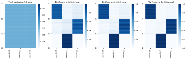
Figure 9: Heatmaps of the matrix ${\mathbf{C}}$ during training on the CIFAR10 dataset. Each row of the matrix denotes the vector ${\mathbf{c}}_{i}$ for a specific client. Darker-colored elements have values closed to $1$.

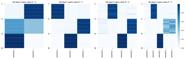
Figure 10: Heatmaps of the final ${\mathbf{C}}$ matrix for different values of $N$ on CIFAR10 dataset. The assignment of subgroups to specific canonical models varies randomly with different values of $N$. For instance, the first canonical model for $N=3$ may learn a distinct subgroup that differs from its assignment when $N=4$.

For the Synthetic dataset, let the vector $\bm{\alpha}_{i}$ represent the ground-truth mixture weight in client $i$ and $\hat{{\mathbf{c}}}_{i}$ be the estimated membership vector. Generally, we hope $\hat{{\mathbf{c}}_{i}}$ be close to the mixture weight $\bm{\alpha}_{i}$ (e.g., if client $i$ has a significant proportion of samples from the $k$-th source, we expect the value of $\hat{c}_{ik}$ to be large). Then, we employ the difference $\frac{\sum_{k=1}^{K}|\alpha_{ik}-\hat{c}_{ik}|}{2}$ to evaluate the gap between the ground-truth mixture weight $\bm{\alpha}_{i}$ and the learned vector $\hat{\mathbf{c}}_{i}$. As shown in Figure 11, the estimated $\hat{\mathbf{c}}_{i}$ gradually approaches the ground-truth mixture weight $\bm{\alpha}_{i}$ along with the increasing of communication round, which demonstrates that PPFL can learn the client’s underlying preference in the mixture distribution scenario.

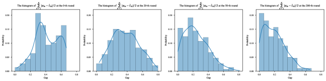
Figure 11: The histogram of $\frac{\sum_{k=1}^{K}|\alpha_{ik}-\hat{c}_{ik}|}{2}$ at different communication rounds for Synthetic dataset. The closer the value is to $0$, the more closely the estimated vector $\hat{\mathbf{c}}_{i}$ approaches the ground-truth mixture weight $\bm{\alpha}_{i}$.

References

- Beck and Teboulle (2003) Amir Beck and Marc Teboulle. Mirror descent and nonlinear projected subgradient methods for convex optimization. Operations Research Letters, 31(3):167–175, 2003.
- Bertsekas (1999) Dimitri P Bertsekas. Nonlinear Programming: 2nd Edition. Athena Scientific, 1999.
- Bonkhoff and Grefkes (2022) Anna K Bonkhoff and Christian Grefkes. Precision medicine in stroke: towards personalized outcome predictions using artificial intelligence. Brain, 145(2):457–475, 2022.
- Bregman (1967) Lev M Bregman. The relaxation method of finding the common point of convex sets and its application to the solution of problems in convex programming. USSR Computational Mathematics and Mathematical Physics, 7(3):200–217, 1967.
- Bryk and Raudenbush (1987) Anthony S Bryk and Stephen W Raudenbush. Application of hierarchical linear models to assessing change. Psychological Bulletin, 101(1):147, 1987.
- Caldas et al. (2018) Sebastian Caldas, Sai Meher Karthik Duddu, Peter Wu, Tian Li, Jakub Konevcnỳ, H Brendan McMahan, Virginia Smith, and Ameet Talwalkar. Leaf: A benchmark for federated settings. arXiv preprint arXiv:1812.01097, 2018.
- Chen et al. (2023) Hong-You Chen, Jike Zhong, Mingda Zhang, Xuhui Jia, Hang Qi, Boqing Gong, Wei-Lun Chao, and Li Zhang. Federated learning of shareable bases for personalization-friendly image classification. arXiv preprint arXiv:2304.07882, 2023.
- Chen et al. (2022) Zixiang Chen, Yihe Deng, Yue Wu, Quanquan Gu, and Yuanzhi Li. Towards understanding the mixture-of-experts layer in deep learning. In Advances in Neural Information Processing Systems, pages 23049–23062, 2022.
- Collins et al. (2021) Liam Collins, Hamed Hassani, Aryan Mokhtari, and Sanjay Shakkottai. Exploiting shared representations for personalized federated learning. In International Conference on Machine Learning, pages 2089–2099, 2021.
- Dang and Lan (2015) Cong D Dang and Guanghui Lan. Stochastic block mirror descent methods for nonsmooth and stochastic optimization. SIAM Journal on Optimization, 25(2):856–881, 2015.
- Dinh et al. (2021) Canh T Dinh, Tung T Vu, Nguyen H Tran, Minh N Dao, and Hongyu Zhang. Fedu: A unified framework for federated multi-task learning with laplacian regularization. arXiv preprint arXiv:2102.07148, 2021.
- Feffer et al. (2018) Michael Feffer, Ognjen Rudovic, and Rosalind W Picard. A mixture of personalized experts for human affect estimation. In Machine Learning and Data Mining in Pattern Recognition, pages 316–330, 2018.
- Feng et al. (2020) Jingshuo Feng, Xi Zhu, Feilong Wang, Shuai Huang, and Cynthia Chen. A learning framework for personalized random utility maximization (rum) modeling of user behavior. IEEE Transactions on Automation Science and Engineering, 19(1):510–521, 2020.
- Fröhlich et al. (2018) Holger Fröhlich, Rudi Balling, Niko Beerenwinkel, Oliver Kohlbacher, Santosh Kumar, Thomas Lengauer, Marloes H Maathuis, Yves Moreau, Susan A Murphy, Teresa M Przytycka, et al. From hype to reality: Data science enabling personalized medicine. BMC Medicine, 16(1):1–15, 2018.
- Gabel and Timoshenko (2022) Sebastian Gabel and Artem Timoshenko. Product choice with large assortments: A scalable deep-learning model. Management Science, 68(3):1808–1827, 2022.
- Ghosh et al. (2020) Avishek Ghosh, Jichan Chung, Dong Yin, and Kannan Ramchandran. An efficient framework for clustered federated learning. In Advances in Neural Information Processing Systems, pages 19586–19597, 2020.
- Hanzely et al. (2023) Filip Hanzely, Boxin Zhao, and mladen kolar. Personalized federated learning: A unified framework and universal optimization techniques. Transactions on Machine Learning Research, 2023.
- He et al. (2016) Kaiming He, Xiangyu Zhang, Shaoqing Ren, and Jian Sun. Deep residual learning for image recognition. In Proceedings of the IEEE Conference on Computer Vision and Pattern Recognition, pages 770–778, 2016.
- Huang et al. (2021) Yutao Huang, Lingyang Chu, Zirui Zhou, Lanjun Wang, Jiangchuan Liu, Jian Pei, and Yong Zhang. Personalized cross-silo federated learning on non-iid data. In AAAI Conference on Artificial Intelligence, pages 7865–7873, 2021.
- Jeong and Hwang (2022) Wonyong Jeong and Sung Ju Hwang. Factorized-fl: Personalized federated learning with parameter factorization & similarity matching. In Advances in Neural Information Processing Systems, pages 35684–35695, 2022.
- Kairouz et al. (2021) Peter Kairouz, H Brendan McMahan, Brendan Avent, Aurélien Bellet, Mehdi Bennis, Arjun Nitin Bhagoji, Kallista Bonawitz, Zachary Charles, Graham Cormode, Rachel Cummings, et al. Advances and open problems in federated learning. Foundations and Trends® in Machine Learning, 14(1–2):1–210, 2021.
- Kamp et al. (2023) Michael Kamp, Jonas Fischer, and Jilles Vreeken. Federated learning from small datasets. In International Conference on Learning Representations, 2023.
- Khan and Yairi (2018) Samir Khan and Takehisa Yairi. A review on the application of deep learning in system health management. Mechanical Systems and Signal Processing, 107:241–265, 2018.
- Krizhevsky (2009) Alex Krizhevsky. Learning multiple layers of features from tiny images. Technical report, University of Toronto, 2009.
- LeCun et al. (1998) Yann LeCun, Léon Bottou, Yoshua Bengio, and Patrick Haffner. Gradient-based learning applied to document recognition. Proceedings of the IEEE, 86(11):2278–2324, 1998.
- Li et al. (2020) Tian Li, Anit Kumar Sahu, Ameet Talwalkar, and Virginia Smith. Federated learning: Challenges, methods, and future directions. IEEE Signal Processing Magazine, 37(3):50–60, 2020.
- Li et al. (2021) Tian Li, Shengyuan Hu, Ahmad Beirami, and Virginia Smith. Ditto: Fair and robust federated learning through personalization. In International Conference on Machine Learning, pages 6357–6368, 2021.
- Liang et al. (2020) P. P. Liang, Terrance Liu, Liu Ziyin, R. Salakhutdinov, and Louis-Philippe Morency. Think locally, act globally: Federated learning with local and global representations. arXiv preprint arXiv:2001.01523, 2020.
- Lin et al. (2017) Ying Lin, Kaibo Liu, Eunshin Byon, Xiaoning Qian, Shan Liu, and Shuai Huang. A collaborative learning framework for estimating many individualized regression models in a heterogeneous population. IEEE Transactions on Reliability, 67(1):328–341, 2017.
- Liu et al. (2021) Bingyan Liu, Yao Guo, and Xiangqun Chen. Pfa: Privacy-preserving federated adaptation for effective model personalization. In Web Conference, pages 923–934, 2021.
- Long et al. (2022) Guodong Long, Ming Xie, Tao Shen, Tianyi Zhou, Xianzhi Wang, and Jing Jiang. Multi-center federated learning: clients clustering for better personalization. World Wide Web, 26:481–500, 2022.
- Marfoq et al. (2021) Othmane Marfoq, Giovanni Neglia, Aurélien Bellet, Laetitia Kameni, and Richard Vidal. Federated multi-task learning under a mixture of distributions. In Advances in Neural Information Processing Systems, pages 15434–15447, 2021.
- McMahan et al. (2017) Brendan McMahan, Eider Moore, Daniel Ramage, Seth Hampson, and Blaise Aguera y Arcas. Communication-efficient learning of deep networks from decentralized data. In Artificial Intelligence and Statistics, pages 1273–1282, 2017.
- Murdoch et al. (2019) W James Murdoch, Chandan Singh, Karl Kumbier, Reza Abbasi-Asl, and Bin Yu. Definitions, methods, and applications in interpretable machine learning. Proceedings of the National Academy of Sciences, 116(44):22071–22080, 2019.
- Nader et al. (2019) Rafic Nader, Alain Bretto, Bassam Mourad, and Hassan Abbas. On the positive semi-definite property of similarity matrices. Theoretical Computer Science, 755:13–28, 2019.
- Pillutla et al. (2022) Krishna Pillutla, Kshitiz Malik, Abdel-Rahman Mohamed, Mike Rabbat, Maziar Sanjabi, and Lin Xiao. Federated learning with partial model personalization. In International Conference on Machine Learning, pages 17716–17758, 2022.
- Qi et al. (2023) Meng Qi, Yuanyuan Shi, Yongzhi Qi, Chenxin Ma, Rong Yuan, Di Wu, and Zuo-Jun Shen. A practical end-to-end inventory management model with deep learning. Management Science, 69(2):759–773, 2023.
- Qin et al. (2013) Zhiwei Qin, Katya Scheinberg, and Donald Goldfarb. Efficient block-coordinate descent algorithms for the group lasso. Mathematical Programming Computation, 5(2):143–169, 2013.
- Sandler et al. (2018) Mark Sandler, Andrew Howard, Menglong Zhu, Andrey Zhmoginov, and Liang-Chieh Chen. Mobilenetv2: Inverted residuals and linear bottlenecks. In IEEE/CVF Conference on Computer Vision and Pattern Recognition, pages 4510–4520, 2018.
- Sattler et al. (2020) Felix Sattler, Klaus-Robert Müller, and Wojciech Samek. Clustered federated learning: Model-agnostic distributed multitask optimization under privacy constraints. IEEE Transactions on Neural Networks and Learning Systems, 32(8):3710–3722, 2020.
- Shazeer et al. (2017) Noam Shazeer, Azalia Mirhoseini, Krzysztof Maziarz, Andy Davis, Quoc V. Le, Geoffrey E. Hinton, and Jeff Dean. Outrageously large neural networks: The sparsely-gated mixture-of-experts layer. In International Conference on Learning Representations, pages 1–19, 2017.
- Smith et al. (2023) Adam N Smith, Stephan Seiler, and Ishant Aggarwal. Optimal price targeting. Marketing Science, 42(3):476–499, 2023.
- Smith et al. (2017) Virginia Smith, Chao-Kai Chiang, Maziar Sanjabi, and Ameet S Talwalkar. Federated multi-task learning. In Advances in Neural Information Processing Systems, pages 4424–4434, 2017.
- Sun et al. (2016) Ying Sun, Prabhu Babu, and Daniel P Palomar. Majorization-minimization algorithms in signal processing, communications, and machine learning. IEEE Transactions on Signal Processing, 65(3):794–816, 2016.
- T Dinh et al. (2020) Canh T Dinh, Nguyen Tran, and Josh Nguyen. Personalized federated learning with moreau envelopes. In Advances in Neural Information Processing Systems, pages 21394–21405, 2020.
- Tan et al. (2022) Alysa Ziying Tan, Han Yu, Lizhen Cui, and Qiang Yang. Towards personalized federated learning. IEEE Transactions on Neural Networks and Learning Systems, (Early Access):1–17, 2022.
- Tuck et al. (2019) Jonathan Tuck, David Hallac, and Stephen Boyd. Distributed majorization-minimization for laplacian regularized problems. IEEE/CAA Journal of Automatica Sinica, 6(1):45–52, 2019.
- Verbeke and Lesaffre (1996) Geert Verbeke and Emmanuel Lesaffre. A linear mixed-effects model with heterogeneity in the random-effects population. Journal of the American Statistical Association, 91(433):217–221, 1996.
- Wu et al. (2021) Ruiyuan Wu, Anna Scaglione, Hoi-To Wai, Nurullah Karakoc, Kari Hreinsson, and Wing-Kin Ma. Federated block coordinate descent scheme for learning global and personalized models. In AAAI Conference on Artificial Intelligence, pages 10355–10362, 2021.
- Xie et al. (2023) Chulin Xie, De-An Huang, Wenda Chu, Daguang Xu, Chaowei Xiao, Bo Li, and Anima Anandkumar. Perada: Parameter-efficient and generalizable federated learning personalization with guarantees. arXiv preprint arXiv:2302.06637, 2023.
- Yan et al. (2023) Yikai Yan, Chaoyue Niu, Yucheng Ding, Zhenzhe Zheng, Shaojie Tang, Qinya Li, Fan Wu, Chengfei Lyu, Yanghe Feng, and Guihai Chen. Federated optimization under intermittent client availability. INFORMS Journal on Computing, (Early Access), 2023.
- Yang et al. (2020) Yi Yang, Shuai Huang, Wei Huang, and Xiangyu Chang. Privacy-preserving cost-sensitive learning. IEEE Transactions on Neural Networks and Learning Systems, 32(5):2105–2116, 2020.
- Yoganarasimhan (2020) Hema Yoganarasimhan. Search personalization using machine learning. Management Science, 66(3):1045–1070, 2020.
- Zhang et al. (2023) Chunxu Zhang, Guodong Long, Tianyi Zhou, Peng Yan, Zijian Zhang, Chengqi Zhang, and Bo Yang. Dual personalization on federated recommendation. In International Joint Conference on Artificial Intelligence, pages 4558–4566, 2023.
- Zhang et al. (2021) Jie Zhang, Song Guo, Xiaosong Ma, Haozhao Wang, Wenchao Xu, and Feijie Wu. Parameterized knowledge transfer for personalized federated learning. In Advances in Neural Information Processing Systems, pages 10092–10104, 2021.
- Zhou and Tang (2020) Yaqin Zhou and Shaojie Tang. Differentially private distributed learning. INFORMS Journal on Computing, 32(3):779–789, 2020.
- Ziko et al. (2020) Imtiaz Ziko, Jose Dolz, Eric Granger, and Ismail Ben Ayed. Laplacian regularized few-shot learning. In International Conference on Machine Learning, pages 11660–11670, 2020.