Analysis of the RMM-01 Market Maker

Abstract

Constant Function Market Makers (CFMMs)are a popular market design for Decentralized Exchanges (DEXs). Liquidity Providers (LPs)supply the CFMMwith assets to enable trades. In exchange for providing this liquidity, an LPreceives a token that replicates a payoff determined by the trading function used by the CFMM. In this paper, we study a time-dependent CFMMcalled RMM-01. The trading function for RMM-01is chosen such that LPsrecover the payoff of a Black–Scholes priced covered call. First, we introduce the general framework for CFMMs. After, we analyze the pricing properties of RMM-01. This includes the cost of price manipulation and the corresponding implications on arbitrage. Our first primary contribution is from examining the time-varying price properties of RMM-01and determining parameter bounds when RMM-01has a more stable price than Uniswap V2. Finally, we discuss combining lending protocols with RMM-01to achieve other option payoffs which is our other primary contribution.

1 Introduction

Blockchains are distributed computing environments that enable the construction of permissionless censorship-resistant systems such as Decentralized Exchanges (DEXs) [1, 2, 3, 4]. Decentralized financial instruments mitigate undesirable power distributions in existing traditional financial markets  [5]. Currently, there are billions of dollars worth of value in Decentralized Finance (DeFi)protocols .

DEXsare programs that run in a decentralized computing environment that automate the function of market makers in traditional financial exchanges  [6]. Distributed computation has a monetary cost quantified on the Ethereum network in units of gas. This constraint provides incentive for simpler market design. One such design is a Constant Function Market Maker (CFMM)which is characterized by it’s unique trading function  [7, 8]. The trading function defines which trades are valid and assigns a price based on the current supply of reserves.

It was proven in  [9] that for any concave, non-negative, non-decreasing payoff function, there exists a corresponding CFMMreplicating that payoff to Liquidity Providers (LPs). These correspondents are called Replicating Market Makers (RMMs). One such example of an RMMis the Black–Scholes covered call RMM, currently implemented as RMM-01by Primitive  [10]. This work will analyze RMM-01.

In section 2, we introduce a formal framework for CFMMsand examine the trading functions of Uniswap V2and RMM-01. Much of this background summarizes work done in  [8]. We present our main results in Section 3. In Section 3.1, we compute the price impact of a swap. Subsequently, in Section 3.2 we derive the cost of price manipulation and examine the implications on arbitrage. In Section 3.3, we evaluate and identify parameter bounds where RMM-01has less price impact than Uniswap V2. Lastly, in Section 3.4, we examine a methodology for composing the RMM-01LPtokens with other DeFimechanisms to achieve the payoffs of other Black–Scholes priced options.

2 Background

First, we will define a CFMMand show how the trading function is used to determine valid trades. This leads to discussion of LPsand how they earn rewards. Since order books are a familiar concept in finance, we describe a CFMMsthat acts as an order book as a means of comparison. Options are another familiar concept which we introduce briefly before defining the CFMMcalled RMM-01that allows LPsto achieve a payoff of a Black–Scholes Covered Call (CC).

2.1 Constant Function Market Makers

In Traditional Finance (TradFi), market makers facilitate the buy-and-sell orders that make up an order book and the two key actors are buyers and sellers. In DeFi, trades are facilitated against the reserves of assets of a CFMMs. For example, suppose we have a collection of $n$ assets (e.g., tokens) that can be exchanged for another. The reserves of $n$ assets $\boldsymbol{R}\in\mathbb{R}^{n}_{+}$ is called an $n$-asset liquidity pool where for every $i\in\{1,\dots,n\}$, the quantity $R_{i}$ represents the quantity of asset $i$ in the pool. Reserves change when trades are executed.

Let $\boldsymbol{\Delta},\boldsymbol{\Lambda}\in\mathbb{R}^{n}_{+}$ be the tendered basket and received basket, respectively. We refer to the tuple, $(\boldsymbol{\Delta}\,,\boldsymbol{\Lambda})\in\mathbb{R}^{n}_{+}\times\mathbb{R}^{n}_{+}$, as a proposed trade. Specifically, $\Delta_{i}$ and $\Lambda_{i}$ denote the amount of asset $i$ tendered. Fees are typically applied to the tendered basket and they are a means of incentivizing users to provide liquidity. We define the fee as a parameter $\gamma\in(0,1]$.

Definition 2.1.

A Constant Function Market Maker (CFMM) is an $n$-asset pool $\mathbb{R}^{n}_{+}$, and a trading function $\varphi$

$$\varphi\colon\mathbb{R}^{n}_{+}\to\mathbb{R}.$$ (1)

Given any $\mathbf{R}$, the value $\varphi(\mathbf{R})=k$ is called the invariant.

CFMMshave two independent actors. Actors who tender a basket of assets $\boldsymbol{\Delta}$ in order to receive a nonzero basket $\boldsymbol{\Lambda}$ are swappers. Actors who provide those assets that can be swapped are called the LPs. Let us first discuss swappers.

Definition 2.2.

Let $(\boldsymbol{\Delta},\boldsymbol{\Lambda})\neq 0$, then this trade is a valid swap if

$$\varphi(\boldsymbol{R}+\gamma\boldsymbol{\Delta}-\boldsymbol{\Lambda})=\varphi(\boldsymbol{R}).$$ (2)

Graphically, definition 2.2 dictates that valid swaps move reserves along the invariant curves where $\varphi=k$. An illustration of these curves is given in Figure 3 for both Uniswap V2and RMM-01. If $\gamma=1$, we see that a swapper is simply paying $\boldsymbol{\Delta}$ in order to receive $\boldsymbol{\Lambda}$. In the case that $\gamma<1$ (which is typical), the trade is accepted based on the discounted tendered basket, $\gamma\boldsymbol{\Delta}$, but the reserves are still increased by the full $\boldsymbol{\Delta}$. This remainder $(1-\gamma)\boldsymbol{\Delta}$ serves to increase the value the LP’s share of the pool which we call a Liquidity Provider Token (LPT). We discuss LPsfurther in Section 2.3.

Suppose that we have only two assets: Token1 and Token2. In TradFi, an order book will provide the last market price for which a trade was executed. This can be thought of as the exchange ratio $S=\frac{\Lambda_{1}}{\Delta_{2}}$. Here, we will assume that asset $i=n$ is the numeraire and that it is some stable reference such as USDC.

Definition 2.3.

Given a CFMMthe price vector is

$$\boldsymbol{P}\coloneqq\nabla\varphi,$$ (3)

the reported price of asset $i$ is

$$p_{i}\coloneqq\frac{P_{i}}{P_{n}},$$ (4)

and the value of the reserves is

$$V\coloneqq\frac{1}{P_{n}}\boldsymbol{P}^{T}\boldsymbol{R}.$$ (5)

Note that since $\varphi$ is a function of the reserves, so is the reported price $p$. In  [7, Section 2.4] the authors compute examples of pricing with two DEXs: Balancer and Curve  [1, 11]. Uniswap V2has the trading function $\varphi_{\textrm{Uni}}(\boldsymbol{R})\coloneqq R_{1}R_{2}$. The associated price is the ratio of the reserves $p_{1}=\frac{R_{2}}{R_{1}}$. For 2-asset pools we will put $p\coloneqq p_{1}$. For more on Uniswap, see  [12].

When a swap occurs on a CFMM, the reserves change. If the invariant curve for a CFMMshas nonzero curvature, the change in reserves necessarily results in a change in price. For a 2-asset pool, we can define the following.

Definition 2.4.

Fix reserves $\boldsymbol{R}=(R_{1},R_{2})$ and (without loss of generality) a valid swap $\Delta_{1}$ for $\Lambda_{2}$, then the price impact due to $\Delta_{1}$ is

$$g(\Delta_{1})=\frac{d\Lambda_{2}}{d\Delta_{1}}.$$ (6)

The above definition appears in  [13] and more recently in  [14]. For example, take $\varphi_{\textrm{Uni}}$ and suppose that $\Delta_{1}>0$, $\Delta_{2}=0$, and that we require $\Lambda_{1}=0$. This is reasonable since round trip trades are never profitable  [8, Section 2.5]. Following Definition 2.2, a valid swap for $\varphi_{\textrm{Uni}}$ satisfies

$$\varphi_{\textrm{Uni}}(\boldsymbol{R})=R_{1}R_{2}=(R_{1}+\gamma\Delta_{1})(R_{2}-\Lambda_{2})=\varphi_{\textrm{Uni}}(\boldsymbol{R}+\gamma\boldsymbol{\Delta}-\boldsymbol{\Lambda})$$ (7)

which implies

$$\Lambda_{2}=\frac{\Delta_{1}R_{2}}{R_{1}+\Delta_{1}}.$$ (8)

Given that the price $p=\frac{R_{2}}{R_{1}}$, we have that the price impact due to $\Delta_{1}$ is

$$g(\Delta_{1})=\frac{\gamma R_{1}R_{2}}{(R_{1}+\gamma\Delta_{1})^{2}}.$$ (9)

One can define a price impact for arbitrary $n$-asset CFMMs, but note that there is not always a unique received basket $\boldsymbol{\Lambda}$ for a given tendered basket $\boldsymbol{\Delta}$.

It has been shown that depending on a price oracle can introduce centralization risk. If a price oracle is manipulated or malfunctions in any way, the financial consequences can be drastic  [15]. Note that the results of  [7] show that arbitrageurs increase market efficiency and can be utilized to mitigate oracle dependencies.

2.2 Order Book Comparison

In TradFi, a common market architecture is an order book. In the order book design, buyers and sellers provide their liquidity in the form of limit orders at a specific price. Here we will examine the collection of CFMMs that describe an order book and see why they have not been used in the design of decentralized exchanges on the Ethereum network.

An order book can be built as a collection of 2-asset CFMMswith a trading function called a constant sum trading function. We define a generic constant sum trading function by

$$\varphi_{\textrm{cs}}(\mathbf{R})=P_{1}R_{1}+P_{2}R_{2}=\boldsymbol{P}^{T}\boldsymbol{R},$$ (10)

such that $P_{1},P_{2}\in\mathbb{R}_{+}$. The constant sum trading function dictates that valid swaps only execute at a single reported price which is akin to a limit order. The constants $P_{1}$ and $P_{2}$ define the price by

$$p_{\textrm{cs}}=\frac{\partial_{1}\varphi_{\textrm{cs}}}{\partial_{2}\varphi_{\textrm{cs}}}=\frac{P_{1}}{P_{2}}$$ (11)

where $\partial_{i}$ is the partial derivative with respect to the $i^{\textrm{th}}$ reserve. A visual is provided in Figure 2.

When building applications on the blockchain, there is a monetary cost of computation. Thus, an on-chain order book becomes prohibitively expensive since it requires an enormous collection of constant sum markets. Instead, a CFMMallows for a continuous range of prices using a single continuous nonlinear trading function. The dominant market architecture for DEXsis nonlinear CFMMs.

2.3 Liquidity Providers

LPstender assets to a pool in exchange they receive a quantity of LPTsrepresenting their share of pool ownership. The LPTcan always be exchanged for reserve assets if an LPwishes to exit their position. Upon exiting, an LPreceives a basket $\boldsymbol{\Lambda}$ for their LPT. Their share is defined by their initial tendered basket $\boldsymbol{\Delta}$ and the accumulated swap fees. For more detail, see [8]. We refer to the actions an LPperforms as liquidity changes.

Swappers and LPshave a symbiotic relationship so long as $\gamma\neq 1$. For any swap $(\boldsymbol{\Delta},\boldsymbol{\Lambda})$ there will be $(1-\gamma)\boldsymbol{\Delta}$ placed into the pool. Hence, swaps increase the amount of the underlying tokens that an LPTis worth. More detail about the change in value for an LPTis given in  [8, Section 2.6].

In CFMMs, the reported price is updated through arbitrage. To capitalize on an arbitrage opportunity, the arbitrageurs must execute swaps on two exchanges and each swap executed by the arbitrageur on a CFMMgenerates fee paid to LPs. This mechanism drives RMM-01to replicate the payoff of a CC. We do not go into the exact detail here, but instead we refer the reader to the original papers  [16, 4] that describes this trading function and its implementation.

A LPexecutes a trade of the form $(\boldsymbol{\Delta},0)$ or $(0,\boldsymbol{\Lambda})$ that modifies the invariant $k$ but not the reported price. Specifically, LPsmust provide or remove liquidity along directions that preserve the gradient of the trading function.

Definition 2.5.

A valid liquidity change is a trade $(\boldsymbol{\Delta}\,,0)$ or $(0,\boldsymbol{\Lambda})$ such that

$$p(\boldsymbol{R})=p(\boldsymbol{R}+\boldsymbol{\Delta})=p(\boldsymbol{R}-\boldsymbol{\Lambda})$$ (12)

The liquidity changes occur along the constant price curves that can be seen in Figure 3 for both Uniswap V2and RMM-01.

2.4 Black-Scholes Option Pricing

The price of a Black–Scholes option depends on the chosen strike price, $K$, and the time until expiration $\tau$ [17]. Once these parameters are chosen, the option’s price changes due to changes in market price $S$ of the underlying asset, the implied volatility $\sigma$ of the underlying , and the time to expiry $\tau$ of the contract.

The value of an option can be given in terms of the variables $d_{1}$ and $d_{2}$ defined as

$$d_{1}(S,\tau)=\frac{\ln(\frac{S}{K})+\frac{1}{2}\sigma^{2}\tau}{\sigma\sqrt{\tau}}\qquad\textrm{and}\qquad d_{2}(S,\tau)=d_{1}-\sigma\sqrt{\tau}.$$ (13)

Note that throughout this paper, we denote the zero-mean unit-variance Gaussian probability density function (PDF), cumulative distribution function (CDF), and quantile functions by $\phi$, $\Phi$, and $\Phi^{-1}$, respectively.

Definition 2.6.

The value of a long call is

$$V_{\textrm{C}}(S,\tau)=S\Phi(d_{1})-K\Phi(d_{2})$$ (14)

and the value of a covered call is

$$V_{\textrm{CC}}(S,\tau)=S\Phi(-d_{1})+K\Phi(d_{2}).$$ (15)

Black–Scholes priced options satisfy a put-call parity  [18] that allows for a put to be priced immediately. The value of a long put is

$$V_{\textrm{P}}(S,\tau)=V_{\textrm{C}}-S+K=K\Phi(-d_{2})-S\Phi(-d_{1}).$$ (16)

2.5 RMM-01

In the paper Replicating Market Makers [16], the authors provide an example of a CFMMthat approximates the payoff of a Black–Scholes CCoption. This trading function was deployed on the Ethereum main-net under the name RMM-01 [4]. At the time of writing, the average total value locked on RMM-01is $550,965.38 and the average daily swap volume is $11,058.58  [19].

The behavior of RMM-01is unlike options in TradFi. Specifically, it is not a means to buy or sell options contracts as it does not act as a market counterparty. An RMM-01pool is initialized when the LPchooses a strike price $K$ (of ETH in USDC), an implied volatility $\sigma$, the time to expiry $\tau$, and adds liquidity to the pool.

Once a pool is created, other LPsare free to provide liquidity to existing pools. Swappers (commonly arbitrageurs) enticed by profit opportunities from pricing discrepancies between RMM-01and another market. Since LPsgrow their position through swap fees, arbitrage is a necessary ingredient for accurate replication of the Black–Scholes CCpayoff that RMM-01claims. As an added benefit, this methodology eliminates the dependence upon an options market counterparty.

Consider the 2-asset pool with the RMM-01trading function given by

$$\varphi_{\textrm{RMM-01}}\coloneqq-K\Phi(\Phi^{-1}(1-R_{1})-\sigma\sqrt{\tau})+R_{2}.$$ (17)

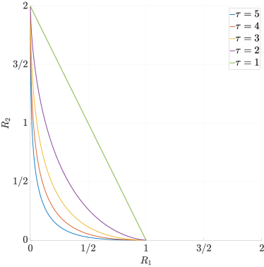
Figure 4: The change in the RMM-01trading curve as $\tau$ varies. We have otherwise fixed $K=2$ and $\sigma=1$.

Token1 is typically called the risky asset (or the underlying in TradFiliterature). Token2 is called the stable asset and is our numéraire. Note that $\varphi_{\textrm{RMM-01}}$ is evaluated on a per-LPTbasis and the invariant $k$ is not a measure of total liquidity as in Uniswap V2. Instead, $k$ measures how accurate the replication of the payoff of a CCis being achieved. We say that there is perfect replication if $k=0$. The pool is over replicating if $k>0$ and under-replicating if $k<0$. We can see how the invariant curves for perfect replication change over time in Figure 4.

3 Properties of RMM-01

Here, we apply some of the definitions from Section 2 to perform analysis on the RMM-01trading function. We first compute the price impact and find the cost of manipulation and associated arbitrage implications. Furthermore, we compare our results to Uniswap V2and introduce a bound on $\sigma\sqrt{\tau}$ in which the trading is preferable on RMM-01. Lastly, we introduce a mechanism to construct additional Black–Scholes priced payoffs.

Equation 17 implies that $R_{1}\in(0,1)$ and if we assume perfect replication it must be that $R_{2}\in(0,K)$ when $\tau>0$. Applying Definition 2.3 to the trading function in Equation 17, the reported price of Token1 in terms of Token2 for an RMM-01pool

$$p=Ke^{\Phi^{-1}(1-R_{1})\sigma\sqrt{\tau}-\frac{1}{2}\sigma^{2}\tau}.$$ (18)

An LPdeposits a collection of Token1 and Token2 in proportional quantities so that the reporting price $p$ from Equation 18 matches the market price $S$. For instance, suppose a user has 1 ETH (Token1) and that the market price for ETH in USDC (Token2) is $S=1000$. Then the reserves of ETH per LPTare given by

$$R_{1}=1-\Phi\left(\frac{\ln\left(\frac{S}{K}\right)+\frac{1}{2}\sigma^{2}\tau}{\sigma\sqrt{\tau}}\right),$$ (19)

which implies that the user will deposit $R_{1}$ ETH. The user can always purchase more or fractional amounts of LPTs. Given the user’s chosen $K$, $\sigma$, and $\tau$, the number of USDC tokens to be deposited is

$$R_{2}=K\Phi\left(\frac{\ln\left(\frac{S}{K}\right)-\frac{1}{2}\sigma^{2}\tau}{\sigma\sqrt{\tau}}\right).$$ (20)

As long as $\sigma\sqrt{\tau}>0$, it follows that $KR_{1}+R_{2}<K$. This means the user may have remaining funds and can choose to purchase more LPTs.

Applying eq. 5 to eq. 17 and assuming $p=S$, we can see the value of RMM-01sLPT$V_{\textrm{{LPT}}}$ in terms of the numeraire $(n=2)$ matches that value of a CC

$$V_{\textrm{{LPT}}} =S\Phi(-d_{1})+K\Phi(d_{2})=V_{\textrm{CC}}.$$ (21)

Briefly, note that when $\tau=0$ (i.e., the pool expired), the trading function becomes a constant sum market

$$KR_{1}+R_{2}=K$$ (22)

and the reported price is

$$p|_{\tau=0}=K.$$ (23)

Recall that a constant sum market is equivalent to a limit order and the geometry is seen in Figure 2.

3.1 Price Impact

Since RMM-01’s trading function changes over time, it follows that the price impact does as well. Also, as RMM-01is not symmetric, we must consider price impacts of both Token1 and Token2 separately. We write $g(\Delta_{1}\,,0)$ and $g(0\,,\Delta_{2})$ to denote the price impacts due to tendering $\Delta_{1}$ and $\Delta_{2}$, respectively.

First, if the swapper tenders $\Delta_{1}$ then Equation 18 implies that the new price $g(\Delta_{1},0)$ is

$$g(\Delta_{1},0)=Ke^{\Phi^{-1}(1-R_{1}-\gamma\Delta_{1})\sigma\sqrt{\tau}-\frac{1}{2}\sigma^{2}\tau}.$$ (24)

At expiry (when $\tau=0$), we have

$$\Lambda_{2}=\frac{\gamma\Delta_{1}}{K},$$ (25)

which implies that swappers can only exchange assets at the strike price when the pool expires. If $S>K$, then all traders are incentivized to convert the pool into Token2, so an LPrecovers their LPTpayoff in Token2. The opposite is also valid, so if $S<K$, the pool expires with only Token1.

If instead, a swapper tenders $\Delta_{2}$, then we can find that the new price is

$$g(0,\Delta_{2})=Ke^{\Phi^{-1}\left(\frac{R_{2}+\gamma\Delta_{2}}{K}\right)+\frac{1}{2}\sigma^{2}\tau}.$$ (26)

Once again, at expiry $p^{\prime}|_{\tau=0}=p|_{\tau=0}$ and we find

$$\Lambda_{1}=\gamma K\Delta_{2}.$$ (27)

3.2 Manipulation and Arbitrage

Suppose that we want to manipulate the reported price from $p\mapsto(1+\epsilon)p$, then we need to find a corresponding $\Delta_{1}$ or $\Delta_{2}$ that would lead to this price change. If the swapper wants to tender $\Delta_{1}$ we use Equations 18 and 24 to see

$$\Delta_{1}=\gamma^{-1}\left(1-R_{1}-\Phi\left(\Phi^{-1}(1-R_{1})+\frac{\ln(1+\epsilon)}{\sigma\sqrt{\tau}}\right)\right).$$ (28)

If $\Delta_{2}$ is tendered then we use Equations 18 and 26 to get

$$\Delta_{2}=\gamma^{-1}K\Phi\left(\Phi^{-1}(1-R_{1})-\sigma\sqrt{\tau}+\frac{\ln(1+\epsilon)}{\sigma\sqrt{\tau}}\right)-\gamma^{-1}R_{2}.$$ (29)

Note that $\Delta_{1}$ and $\Delta_{2}$ are per LPT, thus this cost increases linearly with liquidity. Arbitrageurs also need to execute a swap in order to have the reported price $p$ match an external market price $S$ to maximize their profits. In order for an arbitrageur to initiate a profitable swap, the reported price $p$ must satisfy the following bounds that depend on the fee:

$$\gamma S\leq p\leq\gamma^{-1}S.$$ (30)

These bounds are true for all CFMMs. Given $p$ satisfies the bounds in Equation 30, they can supply $\Delta_{1}$ or $\Delta_{2}$ from Equations 24 and 26 by letting $\epsilon=\gamma^{-1}-1$ if the reported price needs to increase and $\epsilon=\gamma-1$ if the price needs to decrease.

If the invariant curves for a 2-asset trading function have small curvature, then the price impact is also small. More detail on the relationship of curvature to capital efficiency is shown in  [20, 7].

3.3 Compare with Uniswap V2

By comparing RMM-01with Uniswap V2, we can identify explicit bounds for $\sigma\sqrt{\tau}$ such that the price impact for a swap on RMM-01is less than on Uniswap V2. This proves to be useful for users wanting to trade large quantities of assets who don’t want to be exposed to a large price tolerance commonly known as slippage. Existence of these bounds is due to the fact that the curvature of the invariant curves approaches zero for RMM-01as the pool approaches expiry (see Figure fig. 4). We studied price impact in Section 3.2 and in this subsection we examine the price impact with respect to an infinitesimal swap. RMM-01and Uniswap V2have different trading function and consequently price assets differently. Furthermore, RMM-01considers reserves on a per LPTbasis. Suppose that RMM-01and Uniswap V2both report price $p$ for Token1. How do the infinitesimal changes in price for each CFMMrelate to one another? In particular, for what choices of $\sigma$ and $\tau$ can RMM-01achieve less price impact?

Recall that the reported price for Uniswap V2is $p_{\textrm{uni}}=\frac{R_{2}}{R_{1}}$. For any swap tendering either asset, the reserves must be a point along the same invariant curve (see Figure 3). Hence, we can compute a directional derivative of the price along invariant curves to get an infinitesimal price impact. Assuming normalized reserves, $\boldsymbol{P}_{\textrm{Uni}}=\begin{pmatrix}R_{2}&R_{1}\end{pmatrix}^{T}$ which is orthogonal to the invariant curves. We can apply a rotation by $\pi/2$ via a linear transformation $J$ to $\boldsymbol{P}_{\textrm{Uni}}$ yields a vector tangent to the invariant curves $J\boldsymbol{P}_{\textrm{Uni}}=\begin{pmatrix}-R_{1}&R_{2}\end{pmatrix}^{T}$. Computing the directional derivative along $J\boldsymbol{P}_{\textrm{Uni}}$ yields

$$\nabla_{J\boldsymbol{P}_{\textrm{Uni}}}p_{\textrm{uni}}=-R_{1}\frac{\partial p_{\textrm{Uni}}}{\partial R_{1}}+R_{2}\frac{\partial p_{\textrm{Uni}}}{\partial R_{2}}=2p_{\textrm{Uni}}.$$ (31)

By the same argument for RMM-01, we get

$$\nabla_{J\boldsymbol{P}_{\textrm{RMM-01}}}p_{\textrm{RMM-01}}=\frac{p_{\textrm{RMM-01}}\sigma\sqrt{\tau}}{\phi(\Phi^{-1}(1-R_{1}))}.$$ (32)

If we assume $p_{\textrm{Uni}}=p_{\textrm{RMM-01}}$, then we can compare Equations 31 and 32 and determine that for the infinitesimal price impact for RMM-01to be less than that of Uniswap at the same price, it must be that

$$\sigma\sqrt{\tau}<2\phi(\Phi^{-1}(1-R_{1})),$$ (33)

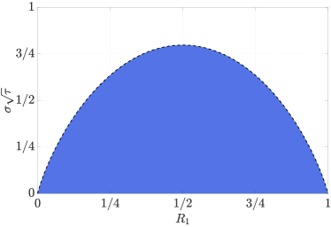
Figure 5: The values for $\sigma\sqrt{\tau}$ where RMM-01’s price impact is less than Uniswap V2.

where $R_{1}$ is the reserves for RMM-01given by Equation 19 and $\phi$ is the standard normal PDF. We can visualize eq. 33 in Figure 5.

3.4 Composability

A natural question is: given the RMM-01LPTcan replicate the payoff of a CC, can one obtain other Black–Scholes priced options from this LPT? We examine the composition of assets and mechanisms that result in the payoff of a long call $V_{\textrm{C}}(S,\tau)$ and consequently a long put. This work expands on some of the results in  [21] which introduces additional composability results from RMM-01.

We propose a basic borrowing and lending mechanism that can achieve the payoff of a long call or put using RMM-01. First, we outline the approach and then we analyze the inherent risk and maximal downsides. Our results illustrate the differences between a traditional call and one built by composing borrowing with RMM-01LPTs. This is a type of trade that can be implemented on blockchains today with no need for a new lending protocol.

In TradFi, put and call options are commonly used to mitigate risk  [22] and they can play a similar role in DeFi. As of March 2022, the derivative market on centralized exchanges for cypto assets represents 62.8% of trading volume [23] expressing an apparent demand.

Assuming perfect replication of RMM-01, the value of an RMM-01LPTis given by $V_{\textrm{CC}}$ found in Equation 15. Since a CCis equivalent to a long position in the underlying and short a call, we get the relationships between $V_{\textrm{CC}}$ and $V_{\textrm{C}}$ seen in Definition 2.6. Using the same relationship, we can achieve the payoff of a call $V_{\textrm{C}}$ by shorting a CCand adding a long position on the underlying. In terms of RMM-01, we must have a method to short the LPTand hold one unit of Token1.

To short an asset in DeFi, one can borrow the asset with collateral and sell it. This sale can be done on a DEXfor either Token1 or Token2. Note that the borrowed asset can be bought back at a later time or the borrowing position can be liquidated. Decentralized lending protocols also ensure at least a one-to-one loan-to-value ratio for collateral and dipping below this ratio causes liquidation. Each of these steps will be called a transaction (labeled $\mathbf{tx}$) and are executed atomically. On a blockchain, collections of transactions are listed onblocks.

For the remainder of this section, assume that $p=S$. Let $\tau_{\textrm{start}}$ be the time of entering the position and $\tau_{\textrm{end}}$ be time of exiting the position such that $\tau_{\textrm{start}}>\tau_{\textrm{end}}\geq 0$. Suppose that a user provides Token1 (e.g., ETH) as collateral in order to borrow an LPT. The user can then immediately sell the LPTfor Token1. Because of atomic execution of transactions, we can assume both transactions occur at $\tau_{\textrm{start}}$. At $\tau_{\textrm{end}}$, the user can buy back the LPTand repay their debt for their original collateral and exit the position unless they have already experienced liquidation. We refer to this position as a RMM-01synthetic call and denote the payoff by $V_{\textrm{RMMC}}$. Thus the steps to construct the $V_{\textrm{RMMC}}$ from the RMM-01LPTare summarized as follows:

Figure 1: Entering the position of a $V_{\textrm{RMMC}}$ at Block: $\tau_{\textrm{start}}$ and exiting it at block Block: $\tau_{\textrm{end}}$.

Note that the position $V_{\textrm{RMMC}}$ described above is built under the assumptions of a one-to-one loan to value ratio. In Table 1 below, the first column denotes $x$ as the sale price of $V_{\textrm{{LPT}}}$ in terms of Token1 at $\tau_{\textrm{start}}$, the second column is the chosen collateral $y\geq x$ provided to borrow the LPT, the third column is the total amount of Token1 the user is exposed to, the fourth column is the value of $V_{\textrm{RMMC}}$ given a market price $S$, and the final column represents the differences between a $V_{\textrm{RMMC}}$ and a $V_{\textrm{C}}$.

Table 1: The positions depending on the CCparameters.

Sale	Col.	Token1	$V_{\textrm{RMMC}}$	$V_{\textrm{C}}-V_{\textrm{RMMC}}$
$x$	$y$	$x+y$	$(x+y)S-V_{\textrm{{LPT}}}$	$(x+y-1)S$

At $\tau_{\textrm{start}}$ it is very possible that $x+y-1\neq 0$. One such case is if the user over-collateralize ($y>x$). However, the user can still achieve the long call payoff by adjusting their exposure to Token1. Specifically, the user needs to find an amount $z$ of Token1 such that $x+y+z-1=0$. The key assumptions are that there is sufficient liquidity of LPTson a lending market and a DEX. The cost of entering the position is the collateral $y$ equal in value to $V_{\textrm{{LPT}}}$ at $\tau_{\textrm{start}}$.

To achieve the payoff of a put, the user replaces all instances of Token1 in Figure fig. 1 with Token2. This is a consequence of put-call parity. Using eq. 16 we can see that $V_{\textrm{P}}=-V_{\textrm{CC}}+K$. In this case, the user may not achieve the correct $+K$ term need due to the value of LPTat $\tau_{\textrm{start}}$.

A loan must have at least a loan-to-value ratio of one which is why it must be that $y\geq x$. The user may provide $y>x$ to ensure that their loan-to-value ratio does not dip below one even with adverse price action of Token1. In essence, the difference $y-x$ can be thought of as a choice of stop-loss. By providing $y=1$, the user can ensure they will never face liquidation since the LPTcan trade for at most one of Token1.

Suppose that the price of Token1 decreases to the point where the LPTexpires containing one of Token1. This is the worst case scenario for the user long $V_{\textrm{RMMC}}$. Then, along the way, the user may find that their loan to value ratio drops below one and they will be liquidated. That is, they will necessarily forfeit their $y$ Token1. They will, however, still keep their $x$ Token1 and can decide what to do from there. At any rate, the maximal loss the user experiences is $yS_{\tau_{\textrm{start}}}$ where $S_{\tau_{\textrm{start}}}$ is the initial price of Token1 in terms of Token2. Once again, this implies the worst possible risk is $S_{\tau_{\textrm{start}}}$ if the user collateralizes using $y=1$.

When an actor borrows assets from a DeFiprotocol, they pay an interest rate on their loan for the time they are borrowing the assets. This means that there is an additional payoff to the lender and an additional cost to the borrower that we do not consider here.

4 Conclusion

In this work, we studied the time-dependent CFMMcalled RMM-01which replicates the payoff of a Black–Scholes CC. Specifically, we computed the price impact due to swaps, discussed price manipulation and arbitrage, and we compared these to known bounds for another CFMMcalled Uniswap V2. Finally, we describe how to achieve the payoff of a long call using an external lending protocol. We do, however, have further open questions to answer.

Optimal Fees for RMM-01.

It has been shown that fixed fees in the RMM-01protocol do not yield perfect replication of a CCpayoff [24]. Since RMM-01has decreasing price impact over time, we believe that the optimal fee mechanism should also decrease over time to allow for larger swaps. Preliminary work has been done here [25].

Symmetric Asset Pools.

Currently RMM-01supports ETH and USDC but it can interact with all ERC20tokens. One potentially interesting research question is to examine the behavior of RMM-01when the pool consists of two stable tokens. The trading function used by Curve  [26] is often used for stable-stable swapping since there is less price impact. Does RMM-01’s time-dependent replication of a CCadd any benefit for a stable-stable pool? Similar to the previous thought, what are the economic implications of a pool consisting of two volatile assets such as ETH and BTC pool?

Appendix A CFMM Geometry

Let us describe the geometry of CFMMtrading curves briefly. First, we can see a visual for the invariant curves for different values of $k$ in the constant sum market trading function $\varphi_{\textrm{cs}}$ described by Equation 10. Alongside this, the price vector $\boldsymbol{P}_{\textrm{cs}}$ is visualized as a vector field. Since the price vector is just a normalized gradient of the trading function $\varphi_{\textrm{cs}}$, $\boldsymbol{P}_{\textrm{cs}}$, it is necessarily orthogonal to the invariant curves. All of this can be seen in Figure 2.

Figure 2: Limit Order as a Constant Sum Market.

We can now look at the invariant curves and the constant price curves for Uniswap V2and RMM-01. The invariant curves consist of the attainable prices for a swapper assuming no fees. By trading a swap with no fees, the values of the reserves are required to change so that the invariant remains constant in Uniswap V2and so that the number of LPTsremain constant for RMM-01. The constant price curves are the curves that an LPwill follow. The amount of reserves tendered or received must maintain the price of the CFMM, hence the name of constant price curves. Moreover, valid liquidity changes will only change the invariant in Uniswap V2and the amount of (or value of) LPTsin RMM-01. Please see the curves in Figure 3.

When there is an included fee $\gamma$, a swapper will swap $\gamma\boldsymbol{\Delta}$ and provide $(1-\gamma)\boldsymbol{\Delta}$ as a liquidity change. That is, $(1-\gamma)\boldsymbol{\Delta}$ will be added by following the constant price curves while $\gamma\boldsymbol{\Delta}$ will be swapped along the invariant curves. This fee will necessarily increase the invariant in Uniswap V2, while in RMM-01the fee will increase the amount of reserves that an LPreceives when they cash-out their LPT.

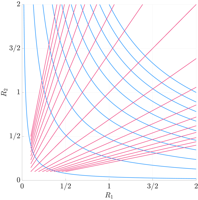
((a)) Curves for Uniswap V2.

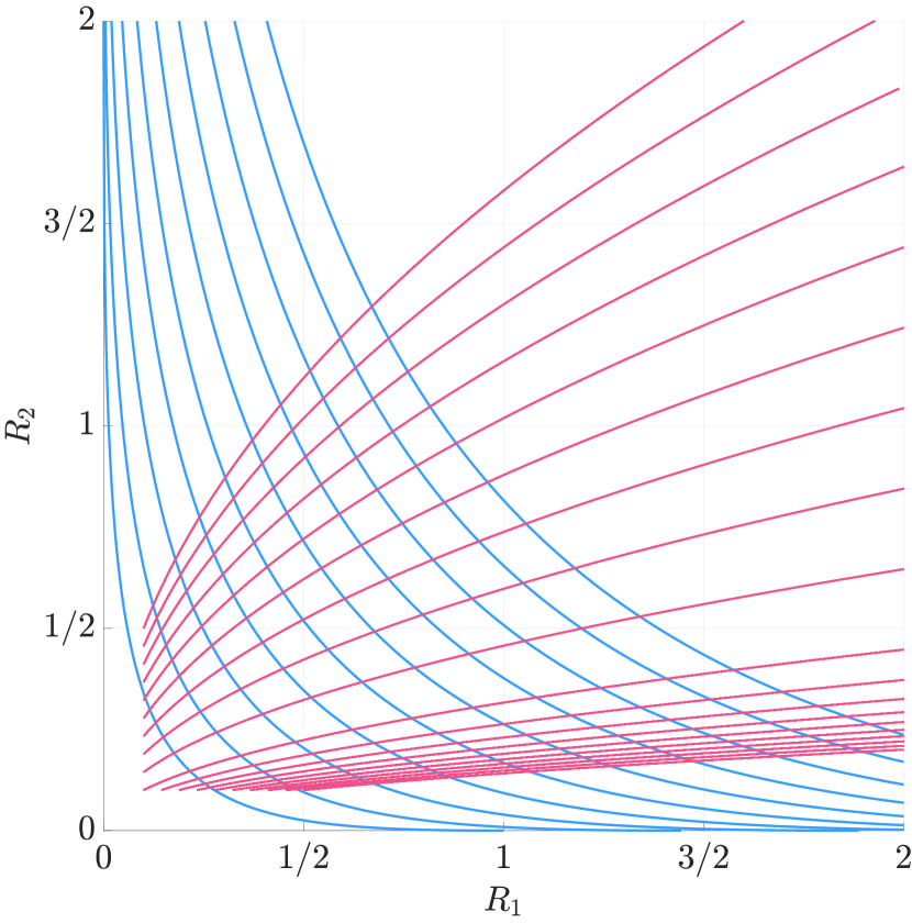
((b)) Curves for RMM-01with $K=2$, $\sigma=1$, and $\tau=5$.

Figure 3: The invariant and constant price curves for two CFMMs.

Appendix B Price Impact and Comparison

The price impact of trades on RMM-01depend heavily on the choice of $\sigma$ and $\tau$. For example, we will always see that as $\tau\to 0$, the price impact approaches zero as well. We can see this algebraically, but visually we have

References

- [1] Ben Hauser. Curvefi/curve-contract: Vyper contracts used in Curve.fi exchange pools. https://github.com/curvefi/curve-contract, May 2021.
- [2] Michael Egorov. StableSwap - efficient mechanism for Stablecoin liquidity. Berkly University, page 6, 2019.
- [3] Noah Zinsmeister and Dan Robinson. Hayden Adams hayden@uniswap.org. Uniswap, page 10, 2020.
- [4] Estelle Sterrett, Alexander Angel, and Matt Czernik. Whitepaper-rmm-01.pdf. https://primitive.xyz/whitepaper-rmm-01.pdf, June 2022.
- [5] Campbell R Harvey, Ashwin Ramachandran, and Joey Santoro. DeFi and the Future of Finance. John Wiley & Sons, 2021.
- [6] Massimo Bartoletti, James Hsin-yu Chiang, and Alberto Lluch-Lafuente. A theory of Automated Market Makers in DeFi, February 2022.
- [7] Guillermo Angeris and Tarun Chitra. Improved Price Oracles: Constant Function Market Makers. In Proceedings of the 2nd ACM Conference on Advances in Financial Technologies, pages 80–91, October 2020.
- [8] Guillermo Angeris, Akshay Agrawal, Alex Evans, Tarun Chitra, and Stephen Boyd. Constant Function Market Makers: Multi-Asset Trades via Convex Optimization. ArXiv, page 31, July 2021.
- [9] Guillermo Angeris, Alex Evans, and Tarun Chitra. Replicating market makers. arXiv q-fin arXiv:2103.14769, 2021.
- [10] Estelle Sterrett, Alexander Angel, Matt Czernik, and experience. Primitive whitepaper. PrimitiveXYZ, 2021.
- [11] Guillermo Angeris, Tarun Chitra, Alex Evans, and Stephen Boyd. Optimal Routing for Constant Function Market Makers, April 2022.
- [12] Guillermo Angeris, Hsien-Tang Kao, Rei Chiang, Charlie Noyes, and Tarun Chitra. An analysis of Uniswap markets, February 2021.
- [13] Guillermo Angeris, Alex Evans, and Tarun Chitra. When does the tail wag the dog? Curvature and market making. ArXiv, page 42, 2022.
- [14] Kshitij Kulkarni, Theo Diamandis, and Tarun Chitra. Towards a Theory of Maximal Extractable Value I: Constant Function Market Makers. ArXiv, page 57, 2022.
- [15] Kevin Tjiam, Rui Wang, Huanhuan Chen, and Kaitai Liang. Your smart contracts are not secure: Investigating arbitrageurs and oracle manipulators in ethereum. In Proceedings of the 3rd Workshop on Cyber-Security Arms Race, pages 25–35, 2021.
- [16] Guillermo Angeris, Alex Evans, and Tarun Chitra. Replicating Monotonic Payoffs Without Oracles, November 2021.
- [17] Fischer Black and Myron Scholes. The pricing of options and corporate liabilities. In World Scientific Reference on Contingent Claims Analysis in Corporate Finance: Volume 1: Foundations of CCA and Equity Valuation, pages 3–21. World Scientific, 2019.
- [18] Robert C. Klemkosky and Bruce G. Resnick. Put-Call Parity and Market Efficiency. The Journal of Finance, 34(5):1141–1155, 1979.
- [19] Kim Evan. Primitivefinance/pool-analytics. https://github.com/primitivefinance/pool-analytics, July 2022.
- [20] Tarun Chitra, Guillermo Angeris, and Hsien-Tang Kao. A Note on Borrowing Constant Function Market Maker Shares. ArXiv, page 16, 2021.
- [21] Estelle Sterrett, Waylon Jepsen, and Evan Kim. Replicating Portfolios: Constructing Permissionless Derivatives, June 2022.
- [22] Kenneth A. Froot, David S. Scharfstein, and Jeremy C. Stein. Risk Management: Coordinating Corporate Investment and Financing Policies. The Journal of Finance, 48(5):1629, December 1993.
- [23] James Webb. Cryptocompare_exchange_review_2022_03_vf-2.pdf. https://www.cryptocompare.com/media/40061772/ cryptocompare_exchange_review_2022_03_vf-2.pdf, 2022.
- [24] The Graph. The GraphiQL. https://api.studio.thegraph.com/query/20803/ primitive-subgraph/v0.0.2-rc0/graphql, January 2022.
- [25] Jason Milionis, Ciamac C Moallemi, Tim Roughgarden, and Anthony Lee Zhang. Automated Market Making and Loss-Versus-Rebalancing. ArXiv, page 21, 2022.
- [26] curve. Curve Documentation. Curve, page 161, June 2022.
- [27] Hayden Adams, Noah Zinsmeister, Moody Salem, River Keefer, and Dan Robinson. Uniswap V3 Core, 2021.