Progress in two-loop electroweak corrections to $gg\to HH$ and $gg\to gH$

Abstract

In these proceedings, we summarise our recent calculations of next-to-leading order electroweak corrections to Higgs boson pair and Higgs boson plus jet production [1, 2]. The calculations are divided into different regions. In the high-energy region, we analytically calculate the Higgs boson contribution to the leading two-loop Yukawa corrections for $gg\to HH$. These corrections are generated by a single virtual Higgs boson exchange within the top quark loop. Our high-energy expansion yields precise predictions for the region where the Higgs boson transverse momenta $p_{T}>120$ GeV. In the low-energy region, we compute the complete two-loop electroweak corrections to $gg\to HH$ and $gg\to gH$. We obtain analytic results through the large top quark mass expansion, covering all sectors of the Standard Model.

1 Introduction

The precise study of spontaneously electroweak (EW) symmetry breaking mechanism of the Standard Model (SM) is one of the primary targets of the Large Hadron Collider (LHC) programme at CERN. In this context, Higgs boson pair and Higgs boson plus jet production are two key processes at the LHC, which have the further potential to reveal new physics effects beyond the SM (BSM). One important feature of the $2\to 2$ Higgs boson production processes is the access to the Higgs boson transverse momenta ($p_{T}$) spectrum, which is known to be sensitive to new physics effects [3]. Moreover, Higgs boson pair production enjoys an additional feature in probing the Higgs self-coupling, which controls the shape of the Higgs potential for the EW symmetry breaking. The determination of the Higgs self-coupling is one of the most important tasks in the upcoming high-luminosity (HL) phase of the LHC. Precise predictions for Higgs boson pair production within the SM is the crucial ingredient for the examination of the EW symmetry breaking mechanism and the detection of subtle effects from BSM scenarios [4, 5].

For Higgs boson pair production at the LHC, the gluon-fusion $gg\to HH$ process represents the major production channel. For this process, the next-to-leading order (NLO) QCD corrections with full top quark mass $m_{t}$ dependence have been calculated in [6, 7, 8, 9, 10]. These QCD calculations involving virtual top quarks are difficult. The successful approaches for tackling this problem are numerical approaches [6, 8, 7] and analytic approximations in complementary regions [9, 11, 12, 10, 13, 14]. However, the calculations of NLO EW corrections are even more involved due to more internal mass scales appearing in the loop integrals, the Higgs self-coupling corrections have been computed in [15], leading Yukawa-top corrections have been computed in high energy expansion [1] and large-$m_{t}$ limit [16], and recently we have computed the first full EW corrections in the large-$m_{t}$ expansion [2].

For Higgs boson plus jet production at the LHC, we consider the dominant gluon-fusion $gg\to gH$ process. For this process, the NLO QCD corrections with full $m_{t}$ dependence are known in [17, 18, 19, 20]. The NLO electroweak corrections via massless bottom quark loops have been computed in [21], the corrections induced by a trilinear Higgs coupling in the large-$m_{t}$ expansion have been calculated in [22], and we have computed the first full EW corrections in the large-$m_{t}$ expansion [2].

In these proceedings, we summarise our progress towards the full NLO EW calculations for $gg\to HH$ and $gg\to gH$ [1, 2].

2 Form factors for $gg\to HH$ and $gg\to gH$

The amplitude for the process $g(q_{1})g(q_{2})\to H(q_{3})H(q_{4})$ can be decomposed into two Lorentz structures

$$A_{1}^{\mu\nu}=g^{\mu\nu}-{\frac{1}{q_{12}}q_{1}^{\nu}q_{2}^{\mu}}\,,\quad A_{2}^{\mu\nu}=g^{\mu\nu}+\frac{1}{{p_{T}^{2}}q_{12}}\left(q_{33}q_{1}^{\nu}q_{2}^{\mu}-2q_{23}q_{1}^{\nu}q_{3}^{\mu}-2q_{13}q_{3}^{\nu}q_{2}^{\mu}+2q_{12}q_{3}^{\mu}q_{3}^{\nu}\right)\,,$$

where $q_{ij}=q_{i}\cdot q_{j}$ with $q_{1}^{2}=q_{2}^{2}=0$ and $q_{3}^{2}=q_{4}^{2}=m_{H}^{2}$, and $p_{T}=\sqrt{(u\,t-m_{H}^{4})/s}\,$ is the Higgs boson transverse momentum. The Mandelstam variables are $s=(q_{1}+q_{2})^{2}\,,t=(q_{1}+q_{3})^{2}\,,u=(q_{1}+q_{4})^{2}\,.$ We introduce the form factors $F_{1}$ and $F_{2}$ as

$${\cal M}^{ab} = \varepsilon_{1,\mu}\varepsilon_{2,\nu}{\cal M}^{\mu\nu,ab}\,\,=\,\,\varepsilon_{1,\mu}\varepsilon_{2,\nu}\delta^{ab}X_{0}^{\rm ggHH}s\left(F_{1}A_{1}^{\mu\nu}+F_{2}A_{2}^{\mu\nu}\right)\,,$$ (1)

where $a,b$ are adjoint colour indices, $X_{0}^{\rm ggHH}=G_{F}\alpha_{s}(\mu)T_{F}/(2\sqrt{2}\pi)$, $T_{F}=1/2$, $G_{F}$ is Fermi’s constant and $\alpha_{s}(\mu)$ is the strong coupling constant evaluated at the renormalization scale $\mu$. In Fig. 1 we show sample two-loop diagrams contributing to $gg\to HH$.

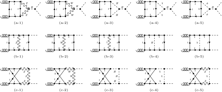
Figure 1: Two-loop Feynman diagrams contributing to $gg\to HH$. Dashed, solid, wavy and curly lines correspond to scalar particles, fermions, electroweak gauge bosons and gluons, respectively.

The amplitude for the process $g(q_{1})g(q_{2})\to g(q_{3})H(q_{4})$ can be decomposed into four physical Lorentz structures

$$A_{1}^{\mu\nu\rho}=g^{\mu\nu}q_{2}^{\rho}\,,\qquad A_{2}^{\mu\nu\rho}=g^{\mu\rho}q_{1}^{\nu}\,,\qquad A_{3}^{\mu\nu\rho}=g^{\nu\rho}q_{3}^{\mu}\,,\qquad A_{4}^{\mu\nu\rho}=\frac{1}{s}q_{3}^{\mu}q_{1}^{\nu}q_{2}^{\rho}\,.$$

The corresponding four form factors are defined through

$${\cal M}^{abc} = f^{abc}X_{0}^{\rm gggH}\varepsilon_{1,\mu}\varepsilon_{2,\nu}\varepsilon_{3,\rho}\sum_{i=1}^{4}F_{i}A_{i}^{\mu\nu\rho}\,,$$ (2)

where $X_{0}^{\rm gggH}=2^{1/4}\sqrt{4\pi\alpha_{s}(\mu)G_{F}}\,\frac{\alpha_{s}(\mu)}{4\pi}\,$, and $c$ is the adjoint colour index of the final-state gluon. The Mandelstam variables are defined as in $gg\to HH$, apart from here we have $q_{3}^{2}=0$ and $p_{T}=\sqrt{u\,t/s}$. Sample Feynman diagrams for $gg\to gH$ are given in Fig. 2.

Figure 2: Two-loop Feynman diagrams contributing to $gg\to gH$. Dashed, solid, wavy and curly lines correspond to scalar particles, fermions, electroweak gauge bosons and gluons, respectively.

We define the perturbative expansion of the form factors as

$$F = F^{(0)}+\frac{\alpha_{s}(\mu)}{\pi}F^{(1,0)}+\frac{\alpha}{\pi}F^{(0,1)}+\cdots\,,$$ (3)

where $\alpha$ is the fine structure constant and the ellipses indicate higher-order QCD and EW corrections.

3 Leading Yukawa corrections to $gg\to HH$ in high energy expansion

As a concrete example, we present the details for the calculation of the leading Yukawa corrections to the Higgs-exchange two-loop box diagram (b-4) shown in Fig. 1. For this diagram, we consider two expansion approaches with the following hierarchies:

$$({\rm A})\,\;s,t\gg m_{t}^{2}\gg(m_{H}^{\rm int})^{2},(m_{H}^{\rm ext})^{2}\quad\mbox{and}\quad({\rm B})\,\;s,t\gg m_{t}^{2}\approx(m_{H}^{\rm int})^{2}\gg(m_{H}^{\rm ext})^{2}\,,$$ (4)

where $m_{H}^{\rm int}$ and $m_{H}^{\rm ext}$ are internal and external Higgs masses respectively. In approach (A) we first treat the hierarchy $m_{t}^{2}\gg(m_{H}^{\rm int})^{2}$ at the level of the integrand by applying the hard-mass expansion procedure using exp [23, 24], and further perform a Taylor expansion in the $m_{H}^{\rm ext}\to 0$ limit. For approach (B) we perform simple Taylor expansions for the hierarchy $m_{t}^{2}\approx(m_{H}^{\rm int})^{2}\gg(m_{H}^{\rm ext})^{2}$. At this stage, the problem is reduced to simpler massive two-loop four-point integrals with massless external lines that only depend on the variables $s$, $t$ and $m_{t}$. We then perform integration-by-parts reductions and derive the system of differential equations for master integrals. To treat the final hierarchy $s,t\gg m_{t}^{2}$, we construct the asymptotic expansion at the level of the master integrals by inserting a power-log ansatz

$$I_{n} = \sum\limits_{i=-3}^{i_{max}}\sum\limits_{j=-4}^{j^{+}}\sum\limits_{k=0}^{i+4}c_{ijk}^{(n)}(s,t)\,\epsilon^{i}\,{m}_{t}^{2j}\,\log^{k}({m}_{t}^{2})\,,$$ (5)

into the system of differential equations w.r.t. $m_{t}$. We then solve the expanded differential equations to a high order in $m_{t}$ in terms of unknown boundary conditions. The boundary conditions need to be calculated analytically from the corresponding master integrals in the limit ${m}_{t}\to 0$. We employ the asymptotic expansion method [25] using asy.m [26] to obtain integral representations for the required boundary conditions. These integrals are subsequently solved using Mellin-Barnes techniques together with our in-house package AsyInt. Finally we obtain analytic results for the amplitudes expanded up to order $m_{t}^{120}$. For the numerical evaluation, we employ the Padé improved approximation to enlarge the radius of convergence of our results.

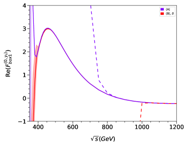
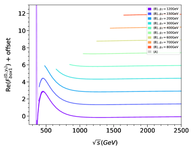
Figure 3: Real part of $F_{\rm box1}$ for fixed scattering angle $\theta=\pi/2$ (left) and different fixed $p_{T}$ values (right). For the fixed $p_{T}$ plot, an offset is applied such that the curves for the different $p_{T}$ values are separated. No offset is used for the lowest $p_{T}$ value. For $p_{T}\geq 120$ GeV the central values of approach (A) and (B) agree.

Here we show results for the real part of box-type form factor of $F_{1}$ for fixed transverse momentum $p_{T}$ and fixed scattering angle in Fig. 3. For the fixed scattering angle plot, the solid curves represent Padé results with uncertainty bands and the dashed curves show naive expansions. We observe that the naive expansions start to diverge for $\sqrt{s}\approx 800$ GeV for approach (A) and for $\sqrt{s}\approx 1000$ GeV for approach (B), while the central value of Padé results agree between both approaches down to $\sqrt{s}\approx 400$ GeV. For the fixed $p_{T}$ plot, the coloured curves correspond to the results from approach (B), and the results from approach (A) are only shown as faint uncertainty bands. These curves show that both expansion approaches yield equivalent physical results.

4 Full EW corrections to $gg\to HH$ and $gg\to gH$ in large-$m_{t}$ expansion

We perform calculations for the full EW corrections to $gg\to HH$ and $gg\to gH$ through the large-$m_{t}$ expansion. To this end, we assume the following hierarchy

$$m_{t}^{2}\gg\xi_{W}m_{W}^{2},\xi_{Z}m_{Z}^{2}\gg s,t,m_{W}^{2},m_{Z}^{2},m_{H}^{2}\,,$$ (6)

where $\xi_{Z}$, $\xi_{W}$ are the general gauge parameters for the $Z$ and $W$ bosons, and perform the large-$m_{t}$ expansion with exp. Through this procedure, we obtain analytic results for the bare two-loop amplitudes up to order $1/m_{t}^{4}$ in the $R_{\xi}$ gauge and order $1/m_{t}^{10}$ $(1/m_{t}^{8})$ in the Feynman gauge for $gg\to HH$ $(gg\to gH)$. For the renormalisation, we express our one-loop amplitudes in terms of independent parameters $\{e,m_{W},m_{Z},m_{t},m_{H}\}$ with $e=\sqrt{4\pi\alpha}$, and introduce one-loop on-shell counterterms. We also renormalise the wave function of the external Higgs boson in the on-shell scheme. Note that tadpole contributions are included in all parts of our calculations. After renormalisation, $\xi_{W}$ and $\xi_{Z}$ drop out for both $gg\to HH$ and $gg\to gH$ amplitudes.

For the numerical evaluation, we adopt the $G_{\mu}$ scheme and use the input values $m_{t}=172~{}\mbox{GeV}\,,m_{H}=125~{}\mbox{GeV}\,,m_{W}=80~{}\mbox{GeV}\,,m_{Z}=91~{}\mbox{GeV}\,,$ and introduce the ratio parameter $\rho_{p_{T}}=\frac{p_{T}}{\sqrt{s}}$. In the following we choose $\rho_{p_{T}}=0.1$ and consider the squared matrix element ${\cal U}_{\rm ggHH}=\frac{1}{8^{2}}\sum_{\rm col}\frac{1}{2^{2}}\sum_{\rm pol}|{\cal M}^{ab}|^{2}=\frac{1}{16}\big{(}X_{0}^{\rm ggHH}s\big{)}^{2}\tilde{{\cal U}}_{\rm ggHH}$ for $gg\to HH$ and ${\cal U}_{\rm gggH}=\frac{1}{8^{2}}\sum_{\rm col}\frac{1}{2^{2}}\sum_{\rm pol}|{\cal M}^{abc}|^{2}=\frac{3}{32}{\big{(}X_{0}^{\rm gggH}\big{)}^{2}s\,\,\tilde{{\cal U}}_{\rm gggH}}$ for $gg\to gH$. The LO and NLO EW numerical results are shown in Fig. 4 for $gg\to HH$ and Fig. 5 for $gg\to gH$ with different expansion order in $m_{t}$. For both processes, our large-$m_{t}$ expansions yield reasonable predictions for the $\sqrt{s}\;\hbox to0.0pt{\lower 3.5pt\hbox{$\mathchar 0\relax\sim$}\hss}\raise 1.0pt\hbox{$<$}\;290$ GeV region. We observe that the NLO EW corrections for $gg\to HH$ can be sizeable, potentially reaching $\mathcal{O}(10\%)$ compared to the LO, while they are small for $gg\to gH$. The analytic NLO QCD results for $gg\to gH$ are also available in [2].

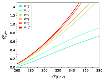
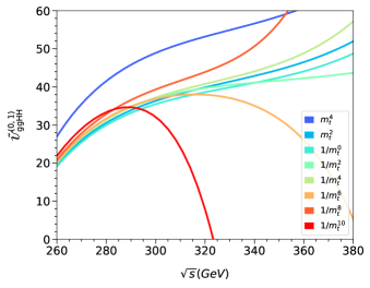
Figure 4: LO $\tilde{{\cal U}}_{\rm ggHH}^{(0)}$ (left) and NLO EW $\tilde{{\cal U}}_{\rm ggHH}^{(0,1)}$ (right) matrix elements plotted as a function of $\sqrt{s}$ for $gg\to HH$. Results are shown up to order $1/m_{t}^{10}$.

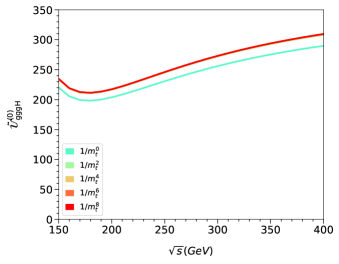
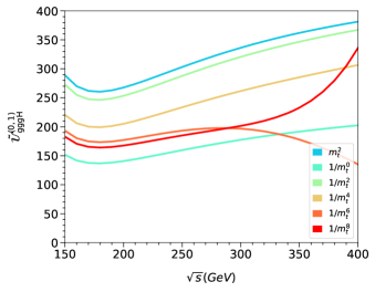
Figure 5: LO $\tilde{{\cal U}}_{\rm gggH}^{(0)}$ (left) and NLO EW $\tilde{{\cal U}}_{\rm gggH}^{(0,1)}$ (right) matrix elements plotted as a function of $\sqrt{s}$ for $gg\to gH$. Results are shown up to order $1/m_{t}^{8}$.

5 Conclusion

In these proceedings, we have summarised our recent analytic calculations of two-loop EW corrections to $gg\to HH$ and $gg\to gH$. We have presented the first NLO leading Yukawa corrections to $gg\to HH$ in the high energy limit. We have proposed two different expansion approaches to tackle this problem and shown that they yield physically equivalent and precise predictions even for Higgs boson $p_{T}$ as small as 120 GeV. We have also presented the first full NLO EW corrections to both $gg\to HH$ and $gg\to gH$ in the large-$m_{t}$ expansion, including all sectors of the SM. Our results also shown that the NLO EW corrections to the $gg\to HH$ can potentially be sizeable.

References

- [1] J. Davies, G. Mishima, K. Schönwald, M. Steinhauser and H. Zhang, JHEP 08 (2022) 259 [2207.02587].
- [2] J. Davies, K. Schönwald, M. Steinhauser and H. Zhang, JHEP 10 (2023) 033 [2308.01355].
- [3] A. Greljo, G. Isidori, J. M. Lindert, D. Marzocca and H. Zhang, Eur. Phys. J. C 77 (2017) 838 [1710.04143].
- [4] H. Abouabid, A. Arhrib, D. Azevedo, J. E. Falaki, P. M. Ferreira, M. Mühlleitner et al., JHEP 09 (2022) 011 [2112.12515].
- [5] S. Iguro, T. Kitahara, Y. Omura and H. Zhang, Phys. Rev. D 107 (2023) 075017 [2211.00011].
- [6] S. Borowka, N. Greiner, G. Heinrich, S. P. Jones, M. Kerner, J. Schlenk et al., Phys. Rev. Lett. 117 (2016) 012001 [1604.06447].
- [7] S. Borowka, N. Greiner, G. Heinrich, S. P. Jones, M. Kerner, J. Schlenk et al., JHEP 10 (2016) 107 [1608.04798].
- [8] J. Baglio, F. Campanario, S. Glaus, M. Mühlleitner, M. Spira and J. Streicher, Eur. Phys. J. C 79 (2019) 459 [1811.05692].
- [9] R. Bonciani, G. Degrassi, P. P. Giardino and R. Gröber, Phys. Rev. Lett. 121 (2018) 162003 [1806.11564].
- [10] J. Davies, G. Heinrich, S. P. Jones, M. Kerner, G. Mishima, M. Steinhauser et al., JHEP 11 (2019) 024 [1907.06408].
- [11] J. Davies, G. Mishima, M. Steinhauser and D. Wellmann, JHEP 03 (2018) 048 [1801.09696].
- [12] J. Davies, G. Mishima, M. Steinhauser and D. Wellmann, JHEP 01 (2019) 176 [1811.05489].
- [13] L. Bellafronte, G. Degrassi, P. P. Giardino, R. Gröber and M. Vitti, JHEP 07 (2022) 069 [2202.12157].
- [14] J. Davies, G. Mishima, K. Schönwald and M. Steinhauser, JHEP 06 (2023) 063 [2302.01356].
- [15] S. Borowka, C. Duhr, F. Maltoni, D. Pagani, A. Shivaji and X. Zhao, JHEP 04 (2019) 016 [1811.12366].
- [16] M. Mühlleitner, J. Schlenk and M. Spira, JHEP 10 (2022) 185 [2207.02524].
- [17] J. M. Lindert, K. Kudashkin, K. Melnikov and C. Wever, Phys. Lett. B 782 (2018) 210 [1801.08226].
- [18] S. P. Jones, M. Kerner and G. Luisoni, Phys. Rev. Lett. 120 (2018) 162001 [1802.00349].
- [19] X. Chen, A. Huss, S. P. Jones, M. Kerner, J. N. Lang, J. M. Lindert and H. Zhang, JHEP 03 (2022) 096 [2110.06953].
- [20] R. Bonciani, V. Del Duca, H. Frellesvig, M. Hidding, V. Hirschi, F. Moriello et al., Phys. Lett. B 843 (2023) 137995 [2206.10490].
- [21] M. Bonetti, E. Panzer, V. A. Smirnov and L. Tancredi, JHEP 11 (2020) 045 [2007.09813].
- [22] J. Gao, X.-M. Shen, G. Wang, L. L. Yang and B. Zhou, Phys. Rev. D 107 (2023) 115017 [2302.04160].
- [23] R. Harlander, T. Seidensticker and M. Steinhauser, Phys. Lett. B 426 (1998) 125 [hep-ph/9712228].
- [24] T. Seidensticker, in 6th International Workshop on New Computing Techniques in Physics Research: Software Engineering, Artificial Intelligence Neural Nets, Genetic Algorithms, Symbolic Algebra, Automatic Calculation, 5, 1999 [hep-ph/9905298].
- [25] M. Beneke and V. A. Smirnov, Nucl. Phys. B 522 (1998) 321 [hep-ph/9711391].
- [26] A. Pak and A. Smirnov, Eur. Phys. J. C 71 (2011) 1626 [1011.4863].
- [27] J. Davies, G. Mishima, M. Steinhauser and D. Wellmann, JHEP 04 (2020) 024 [2002.05558].