Multi-band analyses of the bright GRB 230812B and the associated SN2023pel

Abstract

GRB 230812B is a bright and relatively nearby ($z=0.36$) long gamma-ray burst that has generated significant interest in the community and therefore has been subsequently observed over the entire electromagnetic spectrum. We report over 80 observations in X-ray, ultraviolet, optical, infrared, and sub-millimeter bands from the GRANDMA (Global Rapid Advanced Network for Multi-messenger Addicts) network of observatories and from observational partners. Adding complementary data from the literature, we then derive essential physical parameters associated with the ejecta and external properties (i.e. the geometry and environment) and compare with other analyses of this event (e.g. Srinivasaragavan et al. 2023). We spectroscopically confirm the presence of an associated supernova, SN2023pel, and we derive a photospheric expansion velocity of v $\sim$ 17$\times 10^{3}$ km $s^{-1}$. We analyze the photometric data first using empirical fits of the flux and then with full Bayesian Inference. We again strongly establish the presence of a supernova in the data, with an absolute peak r-band magnitude $M_{r}=-19.41\pm 0.10$. We find a flux-stretching factor or relative brightness $k_{\rm SN}=1.04\pm 0.09$ and a time-stretching factor $s_{\rm SN}=0.68\pm 0.05$, both compared to SN1998bw. Therefore, GRB 230812B appears to have a clear long GRB-supernova association, as expected in the standard collapsar model. However, as sometimes found in the afterglow modelling of such long GRBs, our best fit model favours a very low density environment ($\log_{10}({n_{\rm ISM}/{\rm cm}^{-3}})=-2.16^{+1.21}_{-1.30}$). We also find small values for the jet’s core angle $\theta_{\rm core}={1.70^{+1.00}_{-0.71}}\ \rm{deg}$ and viewing angle. GRB 230812B/SN2023pel is one of the best characterized afterglows with a distinctive supernova bump.

1 Introduction

Gamma-ray bursts (GRBs) are energetic explosions that, with their afterglows, emit over the entire range of electromagnetic radiation. Typically, they are classified in two categories: "long" (duration), lasting more than 2 seconds in the gamma/X-ray bands, and "short", lasting less than 2 seconds. Long GRBs are widely believed to result from the collapse and explosion of a very massive star, hence they are often referred to as "collapsar" and hypernova. Short GRBs are thought to result from the merger of a neutron star with another neutron star or with a black hole (compact objects). In both categories, GRBs produce bipolar jets emerging from the newly formed compact object. The jets interact with the surrounding matter and, through shocks, producing "afterglow" emission, first in the X-ray band, then, as the jet slows and weaker shocks occur, UV, optical, IR, and radio emissions. The luminosity of GRB afterglows is moderately correlated with the isotropic prompt-emission (mostly $\gamma$-ray) energy released, $E_{\rm iso}$ (Gehrels et al., 2008; Nysewander et al., 2009; Kann et al., 2010, 2011).

Core-collapse GRBs are also associated with an optical/near-infrared supernova (SN), which represents the more isotropic outburst (in addition to the jet) from the central explosive process (more below). GRB 980425/SN 1998bw was the first well-documented example of a GRB associated with a supernova, a core-collapse event strongly associated with a (long-duration) burst (Galama et al., 1998; Patat et al., 2001). The association between SN 1998bw and GRB 980425 was first made from the coincidence between the SN’s explosion time and the GRB trigger time (Li & Chevalier, 1999). Moreover, observations of such cases strengthen the fact that galaxies with strong star formation have greater potential for the occurrence of long gamma-ray bursts (Bloom et al., 2002).

In addition to this seminal case, a number of similar associations have been observed since then, such as GRB 030329 with SN 2003dh (Hjorth et al. 2003; Stanek et al. 2003). Spectral features of SN 2003dh indicated a very massive star origin (Deng et al., 2005), reinforcing the notion that the GRB resulted from a core-collapse process. These breakthrough observations opened the door for the collection of a significant number of GRB-SN associations, now a well-identified class of astrophysical events. Other thoroughly studied examples include GRB 031203/SN 2003lw (Malesani et al. 2004), GRB 060218/SN 2006aj (Ferrero et al. 2006; Pian et al. 2006), GRB 100316D/SN 2010bh (Cano et al. 2011), GRB 120422A/SN 2012bz (Melandri et al. 2012; Schulze et al. 2014), GRB 130702A/SN 2013dx (D’Elia et al. 2015), GRB 161219B/SN 2016jca (Ashall et al. 2019), GRB 171010A/SN 2017htp (Melandri et al. 2019), and GRB 200826A (Rossi et al. 2022).

Important elements which strengthen the association of supernovae with gamma-ray bursts (such as the above cases) include the broad lines in the object’s emission spectrum, which are strongly typical of Type Ic supernova lines, and the association with star-forming galaxies; such indicators provide a coherent scenario for the GRB-SN association. Still, important issues remain to be resolved, including: in which cases does a process (collapsar, merger) produce a long or short GRB, and what are their counterpart (r-process or not?); what powers the central engine in each case (magnetar, radioactive heating, etc.); what kinds of jets are produced, etc. To address such key questions, we need a large sample of GRB events exhibiting multi-band emission with a (supernova/kilonova) bump in the light curve, characteristic lines in the spectrum, rich enough data to give us constraints on the current models (radioactive heating, millisecond magnetar central engine, etc.).

Important parameters that characterize the SNe associated with GRBs include their relative brightness $k$ (compared to SN 1998bw), the time of the peak emission (in optical or infra-red), and their "stretch factor" $s$ (or "width") (Cano et al., 2017). A grading system, introduced by (Hjorth & Bloom, 2012) in 2012, became widely adopted for characterizing the strength of a GRB-SN association. The grading ranges from (A), very strong (conclusive spectroscopic evidence), to (E), the weakest associations. In the last 25 years, there have been a dozen cases rated A or A/B (Cano et al., 2017). For those, the average peak time (in the observer frame) is $\sim 13.2$ days (computed from Table 3 of Cano et al. 2017). For these (A or A/B) cases, the relative brightness $k$ ranges from $0.53\pm 0.13$ to $1.81\pm 0.19$, with an average of $1.14\pm 0.21$. The stretch factor $s$ ranges from $0.53\pm 0.11$ to $1.10\pm 0.24$, with an average of $0.84\pm 0.28$ (also computed from Table 3 of Cano et al. 2017).

However, the massive star origin for all long GRBs has recently been challenged by the discovery of a few long GRBs (GRB 211211A, GRB 230307A) associated with a kilonova, normally the signature of a binary compact object merger (Rastinejad et al., 2022; Troja et al., 2022; Yang et al., 2022; Bulla et al., 2023; Levan et al., 2023). In addition to these recent associations with kilonovae, there are also nearby long GRBs without a detected bright SN (Fynbo et al., 2006; Gal-Yam et al., 2006; Valle et al., 2006; Gehrels et al., 2006; Jin et al., 2015). This evidence then produces a much more nuanced picture: while most long GRBs originate in massive star explosions, few may have a different origin. It is thus crucial to obtain a revised census of the collapsar/merger origin for long GRBs. Events at low redshift ($z\lesssim 0.5$) offer an excellent opportunity to carry out this measurement, as the associated SNe, if present, can be easily detected in photometry and even confirmed spectroscopically with 10m-class telescopes. GRB 230812B provided us with an opportunity to further explore these GRB-Supernova/Kilonova associations.

GRB-SN associations may also be found serendipitously with optical wide-field survey programs (Soderberg et al., 2007) rather than by following bursts and their afterglows. GRB 230812B was initially detected by the Fermi Gamma-ray Burst Monitor (GBM - Meegan et al. 2009), the Gravitational wave high-energy Electromagnetic Counterpart All sky Monitor (GECAM), the AGILE/MCAL instrument (Casentini et al. 2023), and the Konus-Wind instrument (Frederiks et al. 2023). This GRB is the most recent event to exhibit a clear SN feature.

Triggered at $T_{0}=$ 18:58:12 UT on 12 August 2023 (GBM trigger 713559497/230812790 - Fermi GBM Team 2023), the GRB’s light curve in the [10 - 10 000] keV band showed a very bright short pulse with a $T_{90}$ duration (90% of its fluence at [50, 300] keV) equal to 3.264 $\pm$ 0.091 s (Roberts et al., 2023). The GECAM light curve reported a value of $T_{90}$ = 4 s in the [6-1000] keV range (Xiong et al., 2023), and Konus $T_{90}$ = 20 s in the [20-1200] keV range (Frederiks et al., 2023), consistent with GBM’s value.The Fermi Large Area Telescope (LAT) independently detected high energy photons with a maximum of 72 GeV ($T_{0}+30$ s) (Scotton et al., 2023).

With the sky localization probability area provided by GBM or LAT (Lesage et al., 2023; Scotton et al., 2023), a series of tiled observations were obtained by the Neil Gehrels Swift observatory X-ray telescope (XRT) (Gehrels et al., 2004), the Zwicky Transient Facility (Salgundi et al., 2023), and the Global MASTER-Net (Lipunov et al., 2023a). The X-ray and UV counterpart of GRB 230812B was discovered 7.1 hours after $T_{0}$ by Swift/XRT (Page & Swift-XRT Team, 2023) and Swift/UVOT (Kuin & Swift/UVOT Team, 2023). The optical counterpart of GRB 230812B was found by the Zwicky Transient Facility on 2023-08-13 at 03:34:56, 8.5 hours after the GRB trigger time T₀ (Salgundi et al., 2023), and also by KAIT (the Katzman Automatic Imaging Telescope - Zheng et al. 2023), which provided localization with arcsecond accuracy. Simultaneously, the Global MASTER-Net robotic telescopes network reported the optical counterpart at the same location (Lipunov et al., 2023b).

A series of photometric observations across the full electromagnetic spectrum were conducted and are still ongoing (at the time of submission of our paper). Among them, we can cite as an example the Multi-purpose InSTRument for Astronomy at Low-resolution spectra-imager (MISTRAL) in optical (Adami et al., 2023a, b; Amram et al., 2023), the Italian 3.6m TNG telescope in near-infrared, and the Northern extended millimeter array (NOEMA) in radio (de Ugarte Postigo et al., 2023b). Spectroscopic observations were also conducted in parallel. It led to the measurements of the transient’s redshift: $z=0.360$ (de Ugarte Postigo et al., 2023a). Twelve days later, observations using OSIRIS+ mounted on the Gran Telescopio Canarias (GTC) showed features in the spectrum characteristic of a GRB-SN event and matched with the spectrum of SN1998bw, indicating, rather conclusively, the presence of a supernova (Agüí Fernández et al., 2023b, a).

Observations with GRANDMA (Global Rapid Advanced Network for Multi-messenger Addicts: Antier et al. 2020a, b; Aivazyan et al. 2022; Kann et al. 2023) observatories started on 2023-08-13T13:34:22, 0.77 days after $T_{0}$, and lasted for 38 days (Mao et al., 2023; Pyshna et al., 2023). In total, more than 20 professional telescopes and several amateur telescopes imaged the source.

GRB 230812B is a high-luminosity and (relatively) close-by burst ($z=0.36$), making it a very worthwhile target of investigation, enabling the study of the correlations between the GRB and SN luminosities, the energy mechanism powering the supernova, etc. Indeed, with a fluence of $3.27\times 10^{-4}$ erg cm^-2 given by Fermi/GBM (Roberts et al., 2023) and the redshift mentioned above, the GRB has a total isotropic gamma energy $E_{\gamma,\rm iso}=8.3\times 10^{52}$ erg; and with the duration ($T_{90}=3.26$ s), one can determine the mean gamma-ray isotropic luminosity $L_{\gamma,\rm iso}=(1+z)E_{\gamma,\rm iso}/T_{90}=3.5\times 10^{52}$ erg s^-1 (Srinivasaragavan et al., 2023), which makes it one of the most luminous GRB-SN events ever recorded.

In this paper, we report observations by the GRANDMA network and its partners of the bright GRB 230812B and the supernova (named SN 2023pel) that emerged in the light curve about five days after the burst onset. In §2, we present the observational data from more than two dozen instruments and the photometric methods we use. We also explore properties from the host galaxy (brightness, line of sight extinction). In §3, we analyse our multi-epoch spectra from the GRB afterglow to the confirmation of the presence of SN2023pel. In §4, we present the methods we applied in the analysis of the afterglow light curves, using both empirical fits and Bayesian inference. We then present our results on the astrophysical scenarios and processes that best describe the data. In §5, we present some general discussion and conclusions.

2 Observational data

2.1 Swift XRT, UVOT

The X-ray light curve ($0.3-10$ keV) of GRB 230812B was acquired from the UK Swift Science Data Centre (Evans et al., 2007, 2009). The data were extracted from the Burst Analyser (Evans et al., 2010), which provides the light curves and spectra of the [0.3-10] keV apparent flux, as well as the unabsorbed flux density at 10 keV in Jansky units. For the spectral energy distribution (SED) fitting to measure the dust from the galaxy (see sections below), the [0.3-10 keV] XRT data were grouped by 10 counts/bin using grppha, a subpackage from HEASoft (version 6.31.1), for statistical purposes. For the other analyses, we performed a re-binning of the unabsorbed light curve at 10 keV by dividing the observations into eight non-continuous time windows. Among these, four windows contained a cluster of observations occurring within an hour or less, while the remaining four had a single data point each. For each cluster, we computed the mean value and standard deviation to produce data points in the light curve for the analysis. These values are reported in Table 6.

We retrieved images taken by the Ultraviolet/Optical Telescope (UVOT, Roming et al. 2005) from the Swift archive. The source was imaged using the broadband white filter from 0.3 days to 8.2 days. In all the images, we checked the effectiveness of the aspect correction. To address the excess broadening induced by pointing jitter from the aging attitude control system (Cenko, 2023), a meticulous assessment of an early image was conducted to determine where the source counts merge into the background. To accommodate this, a slightly larger aperture of 7.5 arcseconds was used for the source. All further images show that the source is contained in this aperture. Background measurements were obtained by analyzing an annular region extending from 10 to 22 arcseconds (after a careful background region positioning). The later images were summed to get a good signal-to-noise ratio in the usual way using the Ftool uvotmaghist. We then transformed the Vega magnitudes to AB magnitudes by adding 0.8 mag as is appropriate in white (Breeveld et al., 2011).

The late-time magnitude upper limits suggest that the host galaxy magnitude is faint, white $>23.2$. We tried deriving a near-UV magnitude for the host galaxy from earlier observations from the Galex gPhoton database, but were unsuccessful in avoiding contamination by nearby stars. We eventually chose the magnitude $23.54\pm 0.84$ in $u$-band from the Sloan Digital Sky Survey DR7 (Abazajian et al., 2009) as an approximation of the white contribution, making sure we propagated properly its very conservative error bars through flux subtraction. The UVOT values, corrected from this constant galaxy flux contribution and from Milky way extinction (see below), are reported in Table 7.

2.2 Optical data set

We conducted simultaneous observations with GRANDMA (Antier et al., 2020a), thanks to its operational platform SkyPortal (Coughlin et al., 2023), and with associated partners, from less than a day after the trigger time $T_{0}$ up to 38 days (see Figure 1). Details on the observational campaign in the various networks can be found in the Appendix. From the images taken, we successfully extracted the photometry of the source and corrected it from the constant flux contribution of the host galaxy and from absorption by dust along the line of sight. The data set can be found in Table 7. Our preliminary analysis of the GRANDMA observations has been reported publicly in the General Coordinates Network (GCN) (Mao et al., 2023; Pyshna et al., 2023).

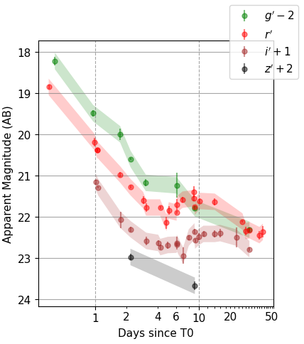
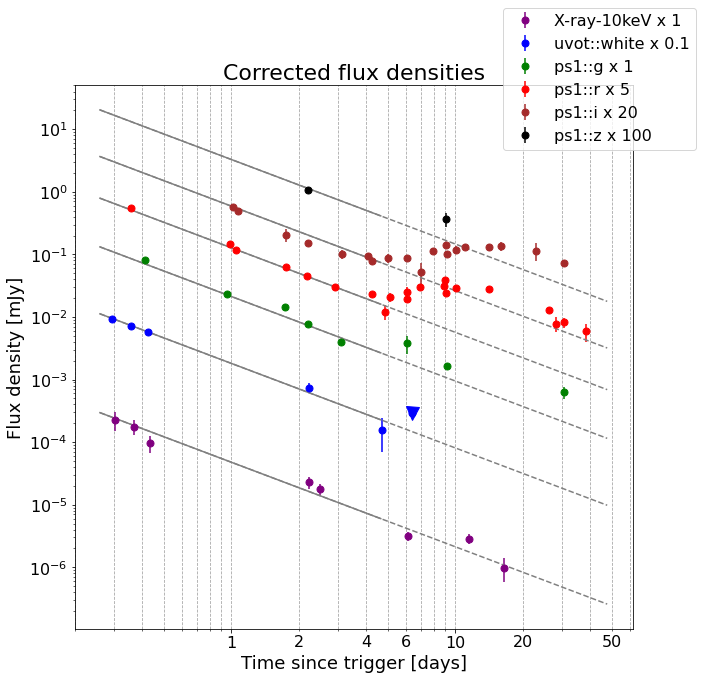
Figure 1: Top: Observations from this work in $g$-, $r$-, $i$-, and $z$-band. Apparent magnitudes before correction by host galaxy flux or for the Milky Way foreground extinction; colored filled regions with arbitrary errorbars 0.2 mag wide have been added to ease the visualization of the light curves. Bottom: Multi-band (X-ray to IR) light curves, corrected from host galaxy flux and the Milky Way foreground extinction. In grey are power-laws fit to the data points up to $T_{0}+5$ days (see section 4.1).

2.2.1 Photometry

Prior to photometry, all images were pre-processed in a telescope-specific way with bias and dark subtraction and flat-fielding. We manually masked the regions of the images containing significant imaging artefacts or regions not fully corrected by the pre-processing. Also, we derived astrometric solutions for the images where telescope pipelines did not provide them by using the Astrometry.net service (Lang et al., 2010).

In order to increase the signal-to-noise ratio of the images, we resampled and coadded individual frames using the Swarp software (Bertin, 2010) for sequences of images acquired on the same telescope within a short interval of time. Then, we performed the forced photometry at the transient position using STDPipe (Karpov, 2021), a set of Python codes for performing astrometry, photometry, and transient detection tasks on optical images, in the same way as Kann et al. (2023).

In order to simplify the analysis and quality checking of the heterogeneous set of images from different telescopes, and to keep track of the results, we created a dedicated web-based application, STDWeb, which acts as a web interface to the STDPipe library and provides a user-friendly way to perform all steps of its data processing, from masking bad regions to image subtraction, with thorough checking of the intermediate results of every step, and then adjusting the settings in order to acquire optimal photometry results. It also contains some heuristics for the selection of an optimal aperture radius and an optimal selection of reference photometric catalogue, refining the astrometric solution as needed, etc.

Specifically, for the photometry on all images, we used an aperture radius equal to the mean FWHM value estimated over all point-like sources in each image. For photometric calibration, we used the Pan-STARRS DR1 catalogue (Flewelling et al., 2016) for processing the images acquired in filters close to the Sloan system. We used a spatially variable photometric zero-point model represented as a second-order spatial polynomial in order to compensate for the effects of improper flat-fielding, image vignetting, and positionally-dependent aperture correction (e.g. due to PSF shape variations). We first performed the analysis taking into account the linear color term (using $g-r$ for Sloan-like filters) in order to assess how much the individual photometric system of the image deviates from the catalogue one. Then, if the color term is negligible (e.g. smaller than $0.1$), we re-run the analysis of the image without the color term, thus directly deriving the measurement in catalogue photometric system. If the color term is significant, we kept it in the analysis and corrected the measurement using the known color of the transient.

When the signal-to-noise ratio obtained with the forced photometry is below 5, we derive an upper limit for it by multiplying the background noise inside the aperture by 5, and converting this flux value to magnitudes. For images taken too close to each other (on a logarithmic timescale), we only selected the one with the best signal-to-noise ratio. Images with a sensitivity too low ($>$ 1.5 apparent magnitude brighter than nearby measurements) were excluded from the data analysis. Images which, after subtraction of the galaxy’s constant flux, give a larger error bar than 0.5, were also excluded from our data set for this analysis.

In parallel, the image reduction for $J$ and $K$ bands was carried out using the jitter task of the ESO-eclipse package. Astrometry was performed using the 2MASS catalogue. Aperture photometry was performed using the Starlink PHOTOM package. To minimize any systematic effect, we performed differential photometry with respect to a selection of local isolated and non-saturated reference stars from the UKIDSS survey.

2.2.2 Host galaxy properties

The host galaxy of GRB 230812B is SDSS J163631.47+475131.8, with measurements available in SDSS DR16 (Ahumada et al., 2020), but its photometry there is marked as unreliable. The host galaxy’s redshift $z=0.36$ was determined through GTC spectroscopic observations of emission lines (de Ugarte Postigo et al., 2023a). We studied its brightness, both for host flux subtraction and spectral analysis.

Constant flux from the host at the location of GRB 230812B – To better characterize the host galaxy flux, we acquired the data for the GRB position from archival Pan-STARRS DR1 (Waters et al., 2020) images in $i^{\prime}$ filters, and from the DESI Legacy Surveys DR10 (Dey et al., 2019) stacked image in $g^{\prime}$, $r^{\prime}$ and $z^{\prime}$ filters. We then performed forced photometry on these images, on the same apertures and with the same parameters as used above for the reduction of the dataset. To convert Legacy Survey measurements to the Pan-STARRS photometric system, we estimated the color term while calibrating these images. For the $g^{\prime}$ filter, this happened to be negligible, but for $r^{\prime}$ and $z^{\prime}$, we used the following equations:

$$r^{\prime}-0.11*(g^{\prime}-r^{\prime})=22.73\pm 0.07$$

$$z^{\prime}-0.11*(r^{\prime}-i^{\prime})=22.31\pm 0.11$$

where the magnitudes $g^{\prime},r^{\prime},i^{\prime},z^{\prime}$ correspond to the Pan-STARRS system. To extract $r^{\prime}$ and $z^{\prime}$, we used the $g^{\prime}$ values estimated from the Legacy Survey image, and $i^{\prime}$ values from Pan-STARRS image. The results are summarized in Table 1. These host flux contributions were then subtracted from the apparent flux to obtain the transient flux, combining the flux errors from the apparent magnitude and the host contribution to obtain the errors on the host-subtracted flux.

In $J$ and $K$ filters, there are to our knowledge no NIR detections of the host in available survey catalogues. We obtained a deep late-time $J$-band observation at $T_{0}+60$ days using the TNG telescope, finding a magnitude of $20.91\pm 0.32$ (Vega), i.e. $21.82$ (AB). This approximate host galaxy contribution could then be subtracted from the other TNG $J$ images. Unfortunately, no late-time imaging in $K$-band could be performed, so no host contribution could be estimated in this filter.

Table 1: Apparent magnitudes of the host galaxy used for flux subtraction and the Milky Way (MW) extinction in the line of sight in different filters.

10 - Filter Host galaxy contribution MW Extinction Magnitude error $u:white$ 23.54 (AB) 0.84 0.099 $g^{\prime}$ 23.78 (AB) 0.12 0.077 $r^{\prime}$ 22.83 (AB) 0.10 0.053 $i^{\prime}$ 22.54 (AB) 0.12 0.040 $z^{\prime}$ 22.34 (AB) 0.12 0.029 $J$ 21.82 (AB) 0.32 0.017 $K$ - 0.007

Star formation rate from the host galaxy – Using these host flux contributions as approximations for the observed magnitude of the galaxy as a whole, we apply the CIGALE code (Boquien et al., 2019) to study the spectral energy distribution (SED) of the galaxy. This analysis constrains the model parameter space to a mass $M=(1.99\pm 0.54)\times 10^{9}M_{\odot}$, a star formation rate (on the last 10 Myr) $SFR=0.17\pm 0.07~{}M_{\odot}\text{yr}^{-1}$, and an attenuation $A_{V}=0.09\pm 0.06$ mag. We show the best-fit spectrum in figure 2. However, one should keep in mind that we are effectively considering the flux of the host galaxy within the aperture size of the transient (a few arcseconds because of point spread of the instruments; to be compared with the $~{}5$ kpc/arcsec scale at $z\simeq 0.36$), and are thus missing a fraction of the galaxy, underestimating the flux by an unknown amount that may bias these galaxy parameters. The SFR is especially hard to constrain without more UV data, so its uncertainty provided here is likely underestimated.

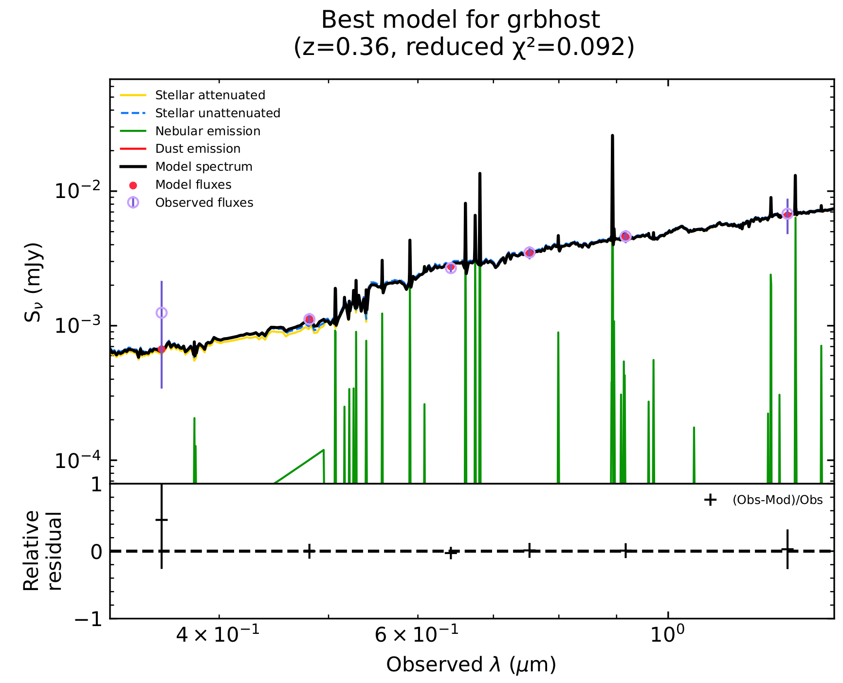
Figure 2: Spectrum of the best-fit host galaxy model in CIGALE, constrained by our estimations in $ugriz$ and $J$ bands.

2.2.3 Line of sight extinction

Milky Way (MW) extinction – We corrected the UV, $griz$, $J$ and $K$ bands from the MW extinction values from Schlafly & Finkbeiner (2011), computed along the line of sight by the NED calculator. These corrections are reported in Table 1.

Host galaxy dust extinction – To estimate the extinction suffered by the afterglow due to the host galaxy dust, we created a spectral energy distribution (SED) from X-ray to optical at two epochs: $T_{0}$ + 2.2 days, corresponding to the quasi-simultaneity of the whitegriz bands, and at $T_{0}$ + 4 days, to include observations from the J, K bands; as no quasi-simultaneous observation was available at this epoch for griJ, the photometric points were estimated through interpolations. We considered the typical extinction curves of MW, Large Magellanic Cloud and Small Magellanic Cloud of Pei (1992), which gave similar results.

We report the results obtained with the average SMC dust extinction law. For each epoch, the intrinsic spectrum was modeled with a single or broken power law using the afterglow theory outlined in Sari et al. (1998). For the broken power law, the difference in slope between X-ray and NIR wavelengths was set to $\Delta\beta$ = $\beta_{X}$ - $\beta_{o}$ = 0.5, which corresponds to the change in slope due to the cooling break. For both epochs, the best fit of the X-ray/NIR SED is obtained with a single power law, and the measured dust extinction $A_{V}$ is compatible with zero (See Table 2). The higher uncertainty in $A_{V}$ for $T{{}_{0}}$ + 4 days is due to higher uncertainties in the $J$- and $K$-band observed fluxes. The best fits of the SED at both epochs are shown in Figure 3.

The $T_{0}$ + 2.2 days SED constrains best the host galaxy dust extinction as $A_{V}=0.0\pm 0.075$ mag, corresponding to a reddening of $E(B-V)=0.0\pm 0.026$ mag for the average SMC model with $R_{V}=2.93$ (this constraint is tighter than but compatible with the upper limit $E(B-V)<0.07$ mag $(3\sigma)$ in Srinivasaragavan et al. 2023). This is consistent with the CIGALE analysis finding a very low global attenuation. We thus chose not to apply any additional extinction correction to the photometric points in Table 7.

Epoch	$A_{V}$ (mag)	$\beta$	$\chi^{2}$ (dof)
$T_{0}$ + 2.2 days	0.0 $\pm$ 0.075	0.710 $\pm$ 0.027	19.269 (7)
$T_{0}$ + 4 days	0.0 $\pm$ 0.185	0.712 $\pm$ 0.036	4.773 (7)

Table 2: Results of the spectral analysis for both epochs.

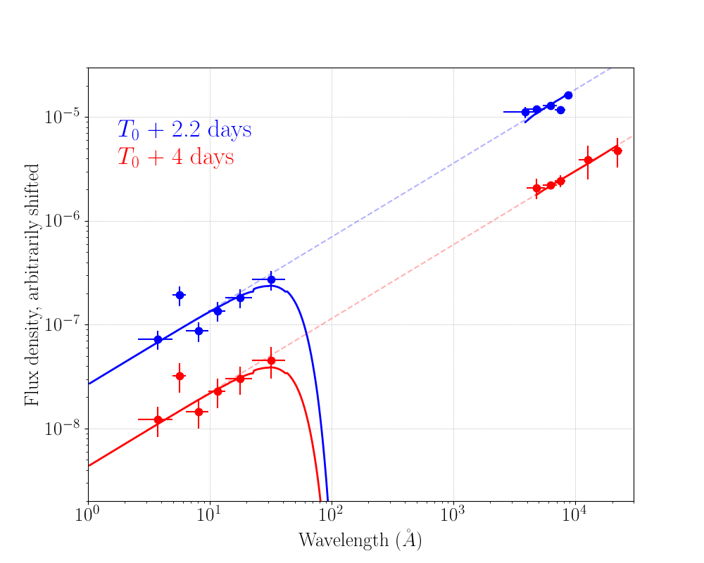
Figure 3: X-ray to NIR SED of the afterglow of GRB 230812B at $T{{}_{0}}$ + 2.2 days and $T{{}_{0}}$ + 4 days. The dashed lines correspond to the best fit intrinsic model (single power law). The solid lines illustrate the best fit to the data, including the absorption in the X-ray. The 0.3-10 keV XRT spectrum extracted around $T{{}_{0}}$ + 2.2 days has been rescaled and used for the SED at $T{{}_{0}}$ + 4 days

2.3 Radio

We also added to our data set two unique submillimeter measurements from NOEMA, takend 3.8 days post $T_{0}$ : see a brief description of the analysis in de Ugarte Postigo et al. (2023b). To complete our multi-wavelength dataset at lower energies, we gathered the published results of radio observations of GRB230812B starting two days after $T_{0}$ and covering different radio bands from 1 to 15.5 GHz. We use the data from the Arcminute Microkelvin Imager Large-Array (Rhodes et al., 2023), the Karl G. Jansky Very Large Array (Giarratana et al., 2023; Chandra et al., 2023), and the upgraded Giant Meterwave Radio Telescope (Mohnani et al., 2023). These data are summarized in Table 6. No correction from the host constant flux and extinction were applied to these measurements.

3 Spectral analysis

We performed spectroscopy of the optical counterpart of GRB 230812B on 3 epochs using OSIRIS+ (Cepa et al., 2000) on the 10.4 m Gran Telescopio Canarias (GTC) (see details in the appendix). These spectra, together with the host galaxy model derived from the SED fit are shown in Fig 4.

The first epoch was obtained 1.1 day after the GRB, when the strong continuum was dominated by the powerlaw, synchrotron emission of the afterglow. As already mentioned by (de Ugarte Postigo et al., 2023a), the spectrum shows a strong trace with both emission and absorption lines which we identify as MgII, MgI, CaII, CaI in absorption, and [OII] and [OIII] in emission, at an average redshift of 0.3602$\pm$0.0006, which we identified as the refined redshift of the GRB. The spectral features and their equivalent widths (EW) are displayed in Table 3. The emission line EWs do not carry much information due to the varying continuum, but the absorption features tell us about the line of sight to the GRB within its own host galaxy. We can calculate the line strength parameter as proposed by de Ugarte Postigo et al. (2012), which determines the strength of the features as compared to the a large sample of afterglows. The line of sight towards GRB 230812B displays a line strength parameter of LSP=0.15$\pm$0.16, indicating that the features are just slightly stronger than the average of the sample (percentile 60 of the sample). The only significant difference with respect to the typical GRB spectrum is the relative strength of MgI with respect to MgII. In our case MgI, is relatively strong, implying that the host galaxy of GRB 230812B is likely to have a low-ionized interstellar environment.

Feature	Obs. wavelength	EW
	Å	Å
MgII	3801.0059	2.55$\pm$0.34
MgII	3811.3960	1.76$\pm$0.27
MgI	3878.7609	2.40$\pm$0.29
$[$OII$]$/$[$OII$]$	5073.5349	-2.26$\pm$0.15
CaII	5353.0027	1.70$\pm$0.16
CaII	5400.9983	1.52$\pm$0.15
CaI	5753.4268	1.23$\pm$0.15
H-beta	6614.7271	-0.93$\pm$0.17
$[$OIII$]$	6750.7251	-0.74$\pm$0.16
$[$OIII$]$	6813.9939	-1.83$\pm$0.15

Table 3: Identification and equivalent width of the spectral features observed in the afterglow spectrum.

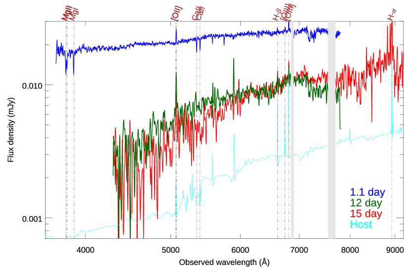
Figure 4: Spectra of GRB 230812B obtained with OSIRIS+. At 1.1 day the emission was dominated by the afterglow, with a simple powerlaw continuum with absorption lines from the line of sight and emission lines from the host. At 12 and 15 days the supernova component is responsible for most of the emission, with little evolution between the two epochs. We have plotted the host galaxy spectrum derived from the SED fit to understand its contribution to the observations.

The other two epochs (12.12 and 15.12 days post $T_{0}$) show similar, broad features typical of broad line Ic supernovae. The second epoch has a slightly redder continuum, that could be due to the cooling of the ejecta.

To analyze the clean SN spectra, we subtracted the contribution from the host galaxy using the host spectrum template that was fit to the host photometry in section 2.2.2. The host subtracted spectra resemble well the ones obtained for SN1998bw at similar rest-frame observing epochs as was earlier noted by Agüí Fernández et al. (2023b), who identify SN2023pel as a broad line type Ic supernova.

Furthermore, we use NGSF (Goldwasser et al., 2022) on the host-subtracted spectra to determine the type of SN associated to the burst. For the spectra taken Aug. 27, the best match was indeed SN 1998bw, at phase 2 days, with a reduced $\chi^{2}=1.79$. We note our second best fit ($\chi^{2}=1.77$) is SN 2002ap, the same found in Srinivasaragavan et al. (2023).

Additionally, we measured the photospheric velocity of SN 2023pel using host-subtracted spectra from GTC. Narrow emission lines and artifacts were first clipped using the IRAF-based routine WOMBAT, and then smoothed the spectra using the the open-source code SESNspectraPCA. We measure the velocity of the Fe II line near the SN peak, a proxy for the photospheric velocity of the SN, using SESNspectraLib (Liu et al., 2016; Modjaz et al., 2016). We measure $v_{ph}=19379\pm 4118$ km s^-1 for the spectrum taken on 2023-08-24 and $v_{ph}=17114\pm 2993$ km s^-1 for the spectrum taken on 2023-08-27. As the latter measurement is closer to the SN peak, we suggest that it is a better proxy for the photospheric velocity of the SN. The velocity we measure is broadly consistent with Srinivasaragavan et al. (2023) and with that of the larger population of GRB-SNe at a similar phase Cano et al. (2017), for which the average velocity at peak is $v=20000\pm 8000$ km/s.

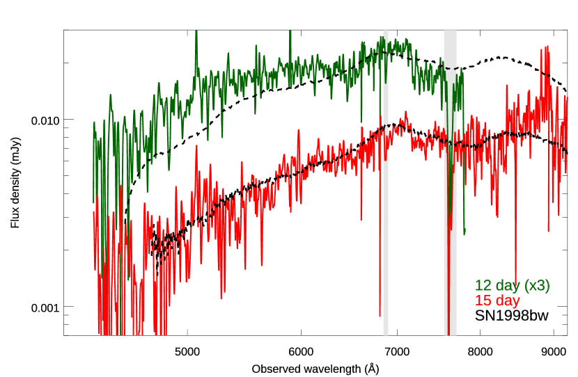
Figure 5: Comparison of the host subtracted spectra of GRB 230812B at times close to the peak of SN2023pel with spectra of SN1998bw at similar rest frame epochs.

4 Multi-wavelength photometric analysis of GRB 230812B and SN 2023pel

4.1 Empirical Light-Curve Analysis

As a first empirical analysis of the afterglow, we perform a multi-band fit of our data up to 5 days (Figure 1, bottom), to avoid including the contribution from the emerging supernova. Assuming a power-law function of the form $F_{\nu}\propto t^{-\alpha}\nu^{-\beta}$, we derive a decay slope of $\alpha=1.35\pm 0.02$ and a spectral slope $\beta=0.74\pm 0.01$ (Figure 6). We note that these values are almost identical to those obtained by Srinivasaragavan et al. (2023) for this GRB: in their work, $\alpha_{o}=1.31\pm 0.02$ and $\beta_{o}=0.74\pm 0.02$. These slopes give an indication of the physical conditions in the GRB’s jet (which produces the afterglow through shocks), particularly the electron distribution’s index $p$ ($N_{e}(E)\propto E^{-p}$).

Using the forward shock model, different assumptions about the afterglow environment lead to different analytical equations $F_{\nu}\propto t^{-\alpha}~{}\nu^{-\beta}$ and relations between $p$ and $\alpha$ and $\beta$ (Sari et al., 1998; Panaitescu & Kumar, 2000). For instance, a fast-cooling scenario describes a spectral index $\beta=p/2$ leading to an unusual $p=1.48\pm 0.03$, but for a slow-cooling scenario, $\beta=(p-1)/2$, which would give a more reasonable $p=2.48\pm 0.03$. For the time-decay slope $\alpha$, a uniform external medium gives $\alpha=(3/4)(p-1)$, which means $p=2.80\pm 0.04$, while a wind medium gives $\alpha=(3p-1)/4$, $p=2.14\pm 0.04$. The temporal and spectral indices are not satisfied by the same value of $p$, thus, a more sophisticated model (e.g. jet with structure) is needed, and that is what the NMMA Bayesian inference analysis will undertake.

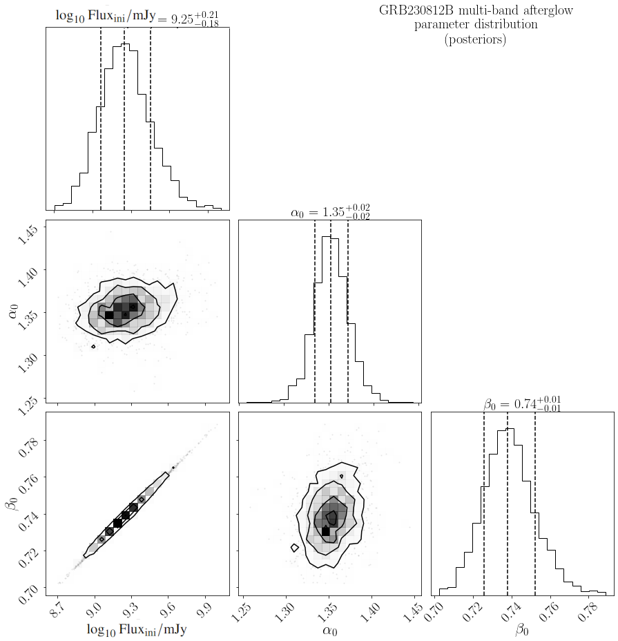
Figure 6: Posteriors of multiband fit of optical afterglow (emission up to 5 days): log of the zero-point flux (at 1 day, 1 Hz, in mJy), temporal decay slope and spectral slope.

4.2 Bayesian Inference using NMMA, investigation of the jet structure and SN contribution

For a physical interpretation of GRB 230812B, we use the Nuclear physics and Multi-Messenger Astronomy framework NMMA (Dietrich et al., 2020; Pang et al., 2022), which is able to perform joint Bayesian inference of multi-messenger events containing gravitational waves, GRB afterglows, SNe, or kilonovae.

Bayesian inference allows us to quantify which theoretical model $\mathbf{M}$ fits the observational dataset $d$ best by computing posterior probability distributions $\mathcal{P}(\vec{\theta})=p(\vec{\theta}|d,\mathbf{M})$. Here $\vec{\theta}$ denotes the model’s parameters. These posteriors are computed via Bayes’ theorem:

$$\mathcal{P}(\vec{\theta})=\frac{p(d|\vec{\theta},\mathbf{M})p(\vec{\theta}|\mathbf{M})}{p(d|\mathbf{M})}=\frac{\mathcal{L}(\vec{\theta})\pi(\vec{\theta})}{\mathcal{Z}(d)}\,,$$ (1)

where $\mathcal{L}(\vec{\theta})$, $\pi(\vec{\theta})$ and $\mathcal{Z}(d)$ are called the likelihood, the prior, and the evidence, respectively. The nested sampling algorithm implemented in pymultinest (Buchner, 2016) is used for obtaining the posterior samples and the evidence.

Assuming a priori that the different scenarios considered are equally likely to explain the data, the plausibility of $\mathbf{M}_{1}$ over $\mathbf{M}_{2}$ is quantified by the Bayes factor

$$\mathcal{B}=\frac{p(d|\mathbf{M}_{1})}{p(d|\mathbf{M}_{2})}\,,$$ (2)

with $\mathcal{B}>1(\ln\mathcal{B}>0)$ indicating a preference for $\mathbf{M}_{1}$, and vice versa. We have analyzed our full data set (X-ray, UV, optical, IR, and radio) with NMMA. All the values quoted in this section are medians with a $95\%$ credible interval as uncertainty.

4.2.1 Confirmation of the GRB+SN scenario

We first establish the statistical significance of the supernova component among other scenarios. Given a set of AB magnitude measurements $\{m^{j}_{i}(t_{i})\}$ (and the associated statistical uncertainties $\sigma^{j}_{i}$) across different times $\{t_{i}\}$ and filters $\{j\}$, the likelihood is given by

$$\mathcal{L}(\vec{\theta})$$ (3)

$$=\prod_{ij}\frac{1}{\sqrt{2\pi((\sigma^{j}_{i})^{2}+(\sigma_{\rm sys})^{2})}}\exp\left(-\frac{1}{2}\frac{\left(m^{j}_{i}-m^{j,{\rm est}}_{i}(\vec{\theta})\right)^{2}}{(\sigma^{j}_{i})^{2}+(\sigma_{\rm sys})^{2}}\right),$$

where $m^{j,\rm{est}}_{i}(\vec{\theta})$ is the estimated AB magnitude for the parameters $\vec{\theta}$ given different models. Moreover, as an improvement over Kunert et al. (2023) and Kann et al. (2023), the systematic uncertainty $\sigma_{\rm sys}$ is treated as a free parameter and sampled over during the nested sampling and not kept fixed at a particular value. Therefore, the resulting posterior of $\sigma_{\rm sys}$ can also be interpreted as the goodness of fit. The lower the $\sigma_{\rm sys}$, the better the fit, and vice versa.

Similar to Kunert et al. (2023) and Kann et al. (2023), we used the semi-analytic code afterglowpy (van Eerten et al., 2010; Ryan et al., 2020) for the GRB afterglow contribution. In this model, the thin-shell approximation is used for handling the dynamics of the relativistic ejecta propagating through the interstellar medium, and the angular structure is introduced by dissecting the blast wave into angular elements, each of which evolves independently, including lateral expansion. The analytical descriptions in Sari et al. (1998) are used for the magnetic-field amplification, electron acceleration, and synchrotron emission from the forward shock. The observed radiation is then computed by performing equal-time arrival surface integration. It should be noted that the model does not account for the presence of a reverse shock or an early coasting phase and does not include inverse Compton radiation. This limits its applicability to the early afterglow of very bright GRBs. In addition, it does not allow to explore a wind-like medium, which may be relevant in a case like GRB230812B with strong evidence for a massive stellar progenitor.

To establish the statistical significance for the presence of the SN component, we compare two models, namely, a GRB with a top-hat jet (Top-hat) and the same GRB with an additional SN component (Top-hat+SN). For the SN component, we use the nugent-hyper model from sncosmo (Levan et al., 2005) with the flux-stretching factor $k_{\rm{SN}}$ and the time-stretching factor $s_{\rm{SN}}$ as the two free parameters. This model is a template constructed from observations of the supernova SN1998bw associated with the long GRB 980425. The resulting log Bayes factor $\ln\mathcal{B}$ of Top-hat+SN against Top-hat is found to be $38.011\pm 0.275$. Based on Jeffreys (1961) and Kass & Raftery (1995), the presence of the SN component is decisively favored against the absence of it.

To verify that the excess power is indeed due to a supernova, rather than some other astrophysical phenomenon, we considered other models. In particular, we considered two kilonova models, Bu2023Ye (Anand et al., 2023) and Ka2017 (Kasen et al., 2017), to accompany the Top-hat model. All of these show similar Bayesian evidence as compared to the Top-hat model, with log Bayes factor $\ln\mathcal{B}<0$. We conclude that none of these models can account for the excess power observed, and the presence of a supernova component is thus statistically supported.

The log Bayes factor $\ln\mathcal{B}$ of various models relative to the Power-law+SN, which is the best-performing model to be introduced shortly, can be found in Table 4. The posterior of $\sigma_{\rm sys}$ is also shown in Table 4. The Power-law+SN has the lowest value of $\sigma_{\rm sys}$, thus signifying a better fit compared to other models.

Scenario	log Bayes factor $\ln\mathcal{B}$	$\sigma_{\rm sys}\ \rm[mag]$
Power-law+SN	ref	$0.140^{+0.062}_{-0.051}$
Top-hat	$-55.388\pm 0.300$	$0.704^{+0.137}_{-0.121}$
Top-hat+SN	$-17.377\pm 0.330$	$0.283^{+0.089}_{-0.079}$
Top-hat+Bu2023Ye	$-55.655\pm 0.300$	$0.708^{+0.136}_{-0.113}$
Top-hat+Ka2017	$-55.490\pm 0.300$	$0.706^{+0.128}_{-0.115}$
Gauss	$-54.888\pm 0.299$	$0.700^{+0.133}_{-0.110}$
Gauss+SN	$-16.615\pm 0.333$	$0.282^{+0.084}_{-0.073}$
Power-law	$-55.064\pm 0.297$	$0.704^{+0.128}_{-0.118}$

Table 4: The log Bayes factor $\ln\mathcal{B}$ and $\sigma_{\rm sys}$ value (median with $95\%$ credible interval) inferred for different models.

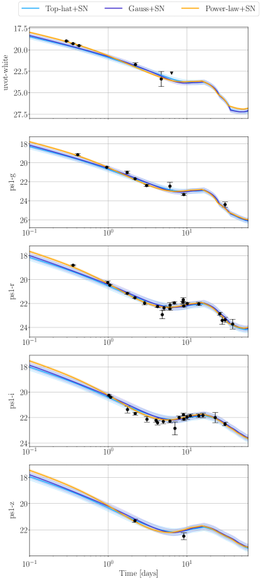
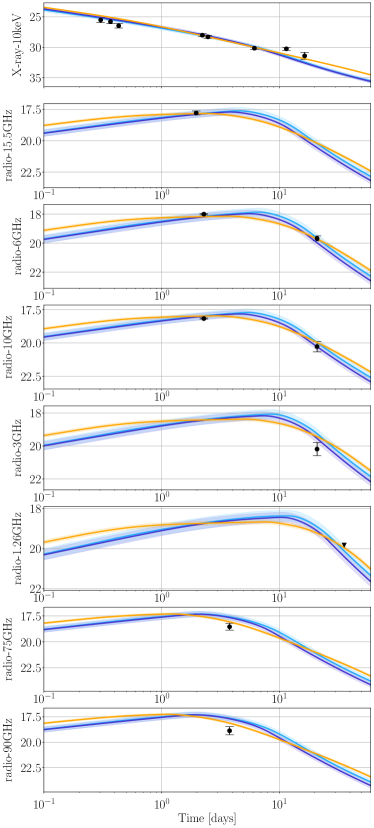
Figure 9: Best-fit light curves for of the GRB + SN models with top-hat, Gaussian and power-law jet structures.

The light curve fits of our best-performing model, i.e. Power-law+SN, are shown in Figure 7. The posterior distributions of the GRB+SN models for all jet structures considered in this work are shown in Figure 8 (corresponding priors in Table 5). The corresponding best-fit light curves are shown in Figure 9 (in the Appendix).

4.2.2 Investigation of the jet structure

We now vary the jet structure of the GRB to try to characterize or to constrain the jet. To do this, we additionally considered Gaussian (Gauss) and power-law (Power-law) jet structures. Gaussian jets feature an angular dependence $E(\theta_{\rm obs})\propto\exp(-\theta_{\rm obs}^{2}/(2\theta_{c}^{2}))$ for $\theta_{\rm obs}\leq\theta_{w}$, with $\theta_{w}$ being an additional free parameter. A power-law jet features an angular dependence $E(\theta_{\rm obs})\propto(1+(\theta_{\rm obs}/\theta_{c})^{2}/b)^{-b/2}$ for $\theta_{\rm obs}\leq\theta_{w}$, with $\theta_{w}$ and $b$ being additional parameters. The resulting log Bayes factor $\ln\mathcal{B}$ of Power-law+SN relative to Tophat+SN and Gauss+SN is found to be $17.377\pm 0.330$ and $16.615\pm 0.333$, respectively.

Given the Bayes factors with the interpretation of Jeffreys (1961) and Kass & Raftery (1995), one will conclude that the power-law jet is decisively favored against the Gaussian and the top-hat jets. Yet, as previously explained, the models presented in afterglowpy have limitations for early-time GRB afterglow, and the early-time data is also the main source of discriminatory power between different jet structures (as seen in Figure 9). Thus one can only conclude that there is a preference for power-law jet structure over top-hat and Gaussian jet structures, but it is not a confirmation for detecting such a structure.

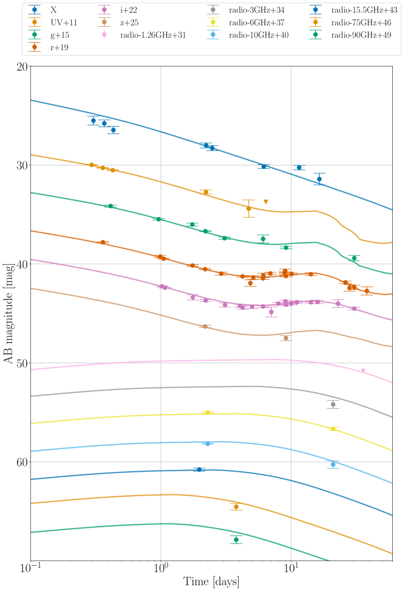
Figure 7: Best-fit light curves of the Power-law+SN model.

In Figure 8, we present the NMMA posteriors for the source parameters, namely the isotropic energy $E_{0}$, the interstellar medium density $n_{\rm ISM}$, the viewing angle $\theta_{\rm obs}$, the half-opening angle of the jet core $\theta_{\rm core}$, and the microphysical parameters $\{p,\epsilon_{e},\epsilon_{B}\}$ (the power-law index of the electron energy distribution, the fraction of energy in electrons, the fraction of energy in the magnetic field, respectively) using the different jet structure models with SN.

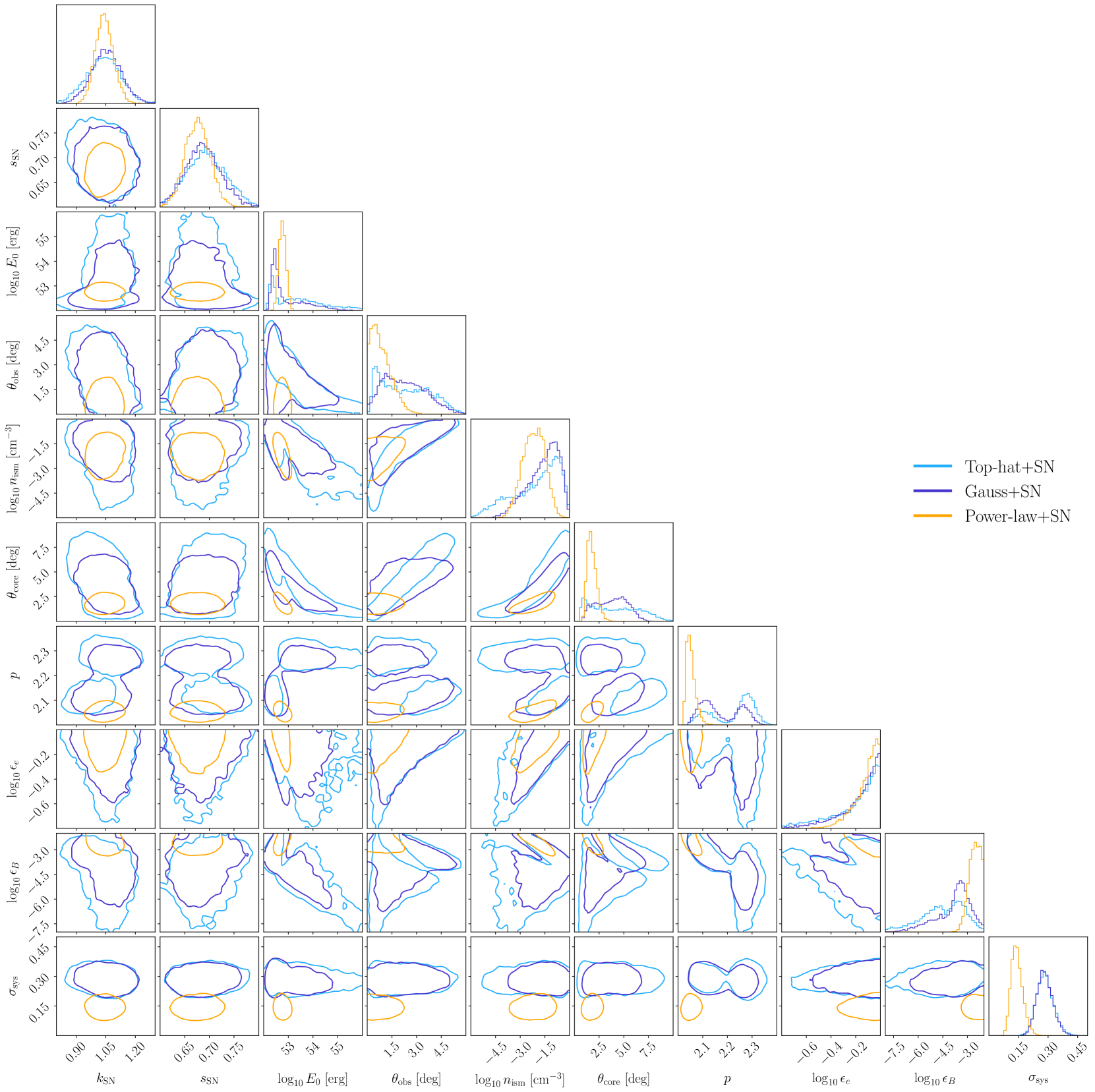
Figure 8: Posterior distribution using different jet models of afterglowpy and nugent-hyper for the supernova component.

The numerical results for the posteriors and the associated priors can be found in Table 5. For the best-fitting model, namely Power-law+SN, the posterior of $p$ gives $p=2.05^{+0.04}_{-0.02}$. Moreover, we find $\log_{10}({E_{0}/{\rm erg}})=52.76^{+0.28}_{-0.26}$ and $\log_{10}({n_{\rm ISM}/{\rm cm}^{-3}})=-2.16^{+1.21}_{-1.30}$ which is rather low. If such an inferred low-density is not uncommon in long GRBs (GRB 990123 - Granot & Taylor 2005; GRB 090510 - Corsi et al. 2010; Joshi & Razzaque 2021; GRB 140515A - Melandri et al. 2015; GRB 160509A - Fraija et al. 2020), it remains surprising in this case where the supernova association is strong evidence for a massive progenitor. This may reflect a strong reduction of the progenitor mass loss in the last centuries before the collapse or that the environment had likely been blown away before the jet’s interaction with it. The fractions of energy in the electrons and in the magnetic field are $\epsilon_{e}=10^{-0.09^{+0.09}_{-0.23}}$ and $\epsilon_{B}=10^{-2.44^{+0.83}_{-0.83}}$; and the jet’s core angle $\theta_{\rm core}={1.70^{+1.00}_{-0.71}}\ \rm{deg}$ and viewing angle $\theta_{\rm obs}={0.75^{+1.27}_{-0.75}}\ \rm{deg}$.

4.2.3 Investigation on the X-ray residual

Figure 7 shows that the best-fitting model has substantial residuals in the X-ray band, especially at earlier times. To further understand this phenomenon, we have performed additional analyses considering data up to 5 days after trigger time, all with the Power-law model, the best-performing GRB model considered. The analyses consider either only the X-ray data or only the UV, optical, and IR (UVOIR) data. The results vary in significance, as demonstrated for instance by the electron energy distribution index $p$. The analysis with the UVOIR dataset gives $p=2.38^{+0.13}_{-0.15}$, whereas the analysis with only X-ray data gives $p=2.27^{+0.22}_{-0.21}$. We should, however, note the limitations of this restricted analysis as it results in posterior distributions that are less constrained due to the lower amount of data considered, in the X-ray band, in particular. Moreover, afterglowpy does not include early-time components such as a reverse shock or inverse Compton radiation. The UVOIR data have a higher weight in the Bayesian analysis due to the higher number of data points in those bands, and since the SN model used here does not support the X-ray band, we can ascribe the high residuals in the X-ray band to a combined effect of the different sizes of the datasets in different filters and a limitation of the models considered in this work.

4.2.4 Comparison of SN1998bw and SN2023pel

Finally, we explore the supernova properties compared to SN1998bw. SN2023pel’s brightness factor $k_{\rm SN}$ and time-stretching factor $s_{\rm SN}$ are found to be, $k_{\rm SN}=1.04^{+0.09}_{-0.09}$ and $s_{\rm SN}=0.68^{+0.05}_{-0.05}$, respectively. For comparison, Srinivasaragavan et al. (2023) find $k_{\rm SN}\approx 0.92$ and $s_{\rm SN}\approx 0.76$. The difference between the inferred stretching factors can be attributed to the difference in the GRB afterglow models being used. The peak apparent (absolute) magnitudes in $r^{\prime}$-band and $i^{\prime}$-band are $21.98^{+0.09}_{-0.10}\ (-19.41^{+0.10}_{-0.09})$ and $21.78^{+0.10}_{-0.29}\ (-18.65^{+0.86}_{-0.67})$, respectively. The corresponding peak time is $15.76^{+0.81}_{-1.21}$ after the trigger for both $r^{\prime}$-band and $i^{\prime}$-band, also consistent with Srinivasaragavan et al. (2023).

Table 5: NMMA - Parameters and prior bounds employed in our Bayesian inferences. We report median posterior values at 95 % credibility for various physical scenarios and jet structures for the GRB. “Uniform” refers to an uniform distribution, and “LogUniform” refers to an uniform distribution for the $\log$ of the parameter. $\mathcal{N}(\mu,\sigma^{2})$ refers to a Gaussian distribution with mean $\mu$ and variance $\sigma^{2}$.

			Top-hat
Parameter	Prior	Prior range		+SN	+Bu2023Ye	+Ka2017	Gauss	Gauss+SN	Power-law	Power-law+SN
(log-) Isotropic afterglow energy $E_{0}$ [erg]	$\rm Uniform$	$[47,57]$	$52.40^{+0.42}_{-0.46}$	$53.28^{+2.39}_{-1.16}$	$52.36^{+0.42}_{-0.41}$	$52.41^{+0.41}_{-0.42}$	$52.63^{+0.78}_{-0.58}$	$52.60^{+1.90}_{-0.41}$	$52.46^{+0.47}_{-0.48}$	$52.76^{+0.28}_{-0.26}$
(log-) Ambient medium’s density $n_{\rm ism}$[$\rm{cm}^{-3}$]	$\rm Uniform$	$[-6,3]$	$-4.76^{+1.47}_{-1.17}$	$-1.68^{+1.57}_{-3.21}$	$-4.81^{+1.32}_{-1.11}$	$-4.87^{+1.36}_{-1.06}$	$-4.66^{+1.65}_{-1.34}$	$-1.41^{+1.25}_{-2.09}$	$-4.78^{+1.46}_{-1.16}$	$-2.16^{+1.21}_{-1.30}$
(log-) Energy fraction in electrons $\epsilon_{\mathrm{e}}$	$\rm Uniform$	$[-5,0]$	$-0.49^{+0.41}_{-0.36}$	$-0.16^{+0.15}_{-0.56}$	$-0.53^{+0.38}_{-0.33}$	$-0.55^{+0.39}_{-0.32}$	$-0.50^{+0.40}_{-0.37}$	$-0.13^{+0.12}_{-0.40}$	$-0.50^{+0.43}_{-0.33}$	$-0.09^{+0.09}_{-0.23}$
(log-) Energy fraction in magnetic field $\epsilon_{\mathrm{B}}$	$\rm Uniform$	$[-10,0]$	$-0.57^{+0.49}_{-0.90}$	$-4.40^{+2.07}_{-3.18}$	$-0.56^{+0.49}_{-0.79}$	$-0.54^{+0.45}_{-0.83}$	$-0.66^{+0.57}_{-1.16}$	$-3.56^{+1.60}_{-2.69}$	$-0.55^{+0.48}_{-0.84}$	$-2.44^{+0.83}_{-0.83}$
Electron distribution power-law index $p$	$\rm Uniform$	$[2.01,3]$	$2.13^{+0.14}_{-0.09}$	$2.26^{+0.08}_{-0.20}$	$2.14^{+0.12}_{-0.09}$	$2.15^{+0.13}_{-0.09}$	$2.15^{+0.14}_{-0.10}$	$2.15^{+0.16}_{-0.09}$	$2.14^{+0.13}_{-0.09}$	$2.05^{+0.04}_{-0.02}$
Viewing angle $\theta_{\rm obs}$ [degrees]	$\mathcal{N}(0,\theta_{\rm core}^{2})$	–	$4.56^{+8.77}_{-4.56}$	$2.19^{+2.68}_{-2.00}$	$3.40^{+6.23}_{-3.40}$	$3.61^{+7.19}_{-3.61}$	$8.01^{+11.61}_{-7.99}$	$2.15^{+2.41}_{-2.08}$	$6.67^{+11.81}_{-6.66}$	$0.75^{+1.27}_{-0.75}$
Jet core’s opening angle $\theta_{\rm core}$ [degrees]	$\rm Uniform$	$[0.6,18]$	$12.96^{+5.04}_{-6.36}$	$3.97^{+4.15}_{-3.38}$	$13.33^{+4.66}_{-5.73}$	$13.05^{+4.94}_{-5.83}$	$10.50^{+7.27}_{-7.30}$	$3.87^{+2.40}_{-2.80}$	$12.16^{+5.84}_{-6.78}$	$1.70^{+1.00}_{-0.71}$
“Wing” truncation angle $\theta_{\rm wing}$ [degrees]	$\rm Uniform$	$[0.6,45]$	–	–	–	–	$28.53^{+16.42}_{-17.77}$	$25.84^{+19.14}_{-17.70}$	$28.88^{+16.12}_{-16.47}$	$20.82^{+18.94}_{-11.93}$
Power-law structure index $b$	$\rm Uniform$	$[0.1,7]$	–	–	–	–	–	–	$3.48^{+3.05}_{-3.37}$	$1.66^{+0.51}_{-0.42}$
Angle ratio $\theta_{\rm obs}/\theta_{\rm core}$	–	–	$0.37^{+0.61}_{-0.35}$	$0.55^{+0.25}_{-0.26}$	$0.28^{+0.37}_{-0.27}$	$0.29^{+0.62}_{-0.29}$	$0.99^{+0.99}_{-0.99}$	$0.65^{+0.42}_{-0.55}$	$0.61^{+0.98}_{-0.60}$	$0.44^{+0.76}_{-0.44}$
Supernova boost $k_{\rm SN}$	$\rm Uniform$	$[0.01,100]$	–	$1.04^{+0.16}_{-0.17}$	–	–	–	$1.05^{+0.15}_{-0.15}$	–	$1.04^{+0.09}_{-0.09}$
Supernova stretch $s_{\rm SN}$	$\rm Uniform$	$[0.1,5.0]$	–	$0.69^{+0.08}_{-0.07}$	–	–	–	$0.69^{+0.07}_{-0.07}$	–	$0.68^{+0.05}_{-0.05}$
Systematic error $\sigma_{\rm sys}$	$\rm LogUniform$	$[0.01,2.0]$	$0.70^{+0.14}_{-0.12}$	$0.28^{+0.09}_{-0.08}$	$0.71^{+0.14}_{-0.11}$	$0.71^{+0.13}_{-0.12}$	$0.70^{+0.13}_{-0.11}$	$0.28^{+0.08}_{-0.07}$	$0.70^{+0.13}_{-0.12}$	$0.14^{+0.06}_{-0.05}$

5 Discussion and Conclusion

GRB 230812B was a bright and relatively nearby gamma-ray burst that displayed a number of important features: it was accompanied by a luminous supernova, it produced radiation from a high energy of 72 GeV down to radio wavelengths, and it continues to be observed more than two months since the initial burst, which was detected by several space detectors. Dozens of images and measurements were taken from observatories across the world, including some 80 data points from our GRANDMA network and partner institutions, necessitating not only careful reductions and analyses but also subtractions of backgrounds, host and Milky Way galaxy absorption (dust) and extinction corrections, etc.

With a duration $T_{90}$ of 3.264 $\pm$ 0.091 s (in the [50 - 300] keV band), GRB 230812B falls in the "long" category, thus (in principle) the result of a very massive star’s collapse, which produces powerful jets and (at least sometimes) a more isotropic supernova, which may be detected several days after the initial burst and afterglow. However, motivated by recent cases indicating that "long" GRBs may sometimes display kilonova characteristics (which are normally associated with "short", merger-type GRBs) and vice versa ("short" GRBs displaying collapsar-type characteristics), it was worthwhile to analyze this GRB’s multi-band emission to see if it is best fit with a supernova or a kilonova, in addition to determining its jet properties, i.e. geometry (observed and core angle) and physical parameters (electron and magnetic field energy fractions, etc.).

In a nutshell, our analyses (using both empirical fits, as explained in §4.1, and the NMMA framework as described in §4.2) found a clear confirmation of a supernova (our data-fitting models with a supernova decisively outperforming models without a supernova or with a kilonova), and a GRB best fit by a high (but not abnormal) total energy $E_{0}=10^{52.76^{+0.28}_{-0.26}}$ erg. SN2023pel peaked $15.76^{+0.81}_{-1.21}$ days (in the observer frame) after the trigger (in both $r^{\prime}$ and $i^{\prime}$ bands), similar to values for cases of strong GRB-SN associations (Cano et al. 2017) and consistent with Srinivasaragavan et al. (2023) for this supernova.

Moreover, relative to SN1998bw (commonly used as a benchmark in GRB-SN cases), SN2023pel had a brightness or flux-stretching factor $s_{\rm SN}=1.04^{+0.09}_{-0.09}$ and a time-stretching factor $k_{\rm SN}=0.68^{+0.05}_{-0.05}$, that is about as bright as SN1998bw but evolving faster, and similar to values found in other strong GRB-SN associations (Cano et al. 2017; Cano 2014). Our best-fit model also gave a very low ambient density $n_{\rm ISM}=10^{-2.16^{+1.21}_{-1.30}}$ cm^-3, similar to a number of previously modeled cases (see the brief discussion and references given above). Further investigations with different models are called for to confirm and understand all these findings.

Our NMMA framework/simulation also gave best-fit parameter values for the jet’s geometry (shape and core and viewing angles) and physical conditions (electron energy distribution index, electron energy fraction, and magnetic field energy fraction). The jet’s geometry/shape was best described by the (angular) ‘power-law’ model; the electron energy distribution index $p$ was found to be $\approx 2.1$, which is quite typical; the best-fit magnetic field energy fraction $\epsilon_{B}$ was $\approx 10^{-2.4}$, also quite typical. However, the electron energy fraction was found to be rather high: $\epsilon_{e}\approx 0.5-1$ ($10^{-0.09^{+0.09}_{-0.23}}$). The jet’s core and viewing angles were found to be small: $\theta_{\rm core}={1.70^{+1.00}_{-0.71}}\ \rm{deg}$ and $\theta_{\rm obs}={0.75^{+1.27}_{-0.75}}\ \rm{deg}$, respectively. Despite these atypical values, the parameters still allow an on-axis jet scenario.

GRB 230812B, bright and relatively close-by, provided us (the GRANDMA network and its partners) the opportunity to perform dozens of observations in UV, optical, near infrared, and sub-millimeter resulting in some 80 high-quality data points. The light curves in optical showed a distinctive supernova bump, SN2023pel, which turned out to be about as bright as the famous SN1998bw. Our spectroscopic analysis determined a photospheric velocity $v_{ph}=17114\pm 2993$ km s^-1 near the peak, and the host-subtracted spectra was best fit by SN1998bw.

The rich data that we have produced, coupled with data from other groups (Srinivasaragavan et al. 2023) and facilities, will help explore this event and other GRB-SN associations with additional tools and models. Covering 9 orders of magnitude in frequency, our multi-band analysis presented some information about the jet and the supernova, but further investigations can help confirm or refine our results.

Data availability

Images and raw data are available upon request.

Affiliations

¹ IJCLab, Univ Paris-Saclay, CNRS/IN2P3, Orsay, France
² Nikhef, Science Park 105, 1098 XG Amsterdam, The Netherlands
³ Institute for Gravitational and Subatomic Physics (GRASP), Utrecht University, Princetonplein 1, 3584 CC Utrecht, The Netherlands
⁴ Physics Department, American University of Sharjah, Sharjah, UAE
⁵ National Research Institute of Astronomy and Geophysics (NRIAG), 1 El-marsad St., 11421 Helwan, Cairo, Egypt
⁶ Aix Marseille Univ, CNRS, CNES, LAM Marseille, France
⁷ Instituto de Astrofísica de Andalucía, Glorieta de la Astronomía s/n, 18008 Granada, Spain
⁸ Cahill Center for Astrophysics, California Institute of Technology, Pasadena CA 91125, USA
⁹ E. Kharadze Georgian National Astrophysical Observatory, Mt. Kanobili, Abastumani, 0301, Adigeni, Georgia
¹⁰ Samtskhe-Javakheti State University, Rustaveli Str. 113, Akhaltsikhe, 0080, Georgia
¹¹ School of Physics and Astronomy, University of Minnesota, Minneapolis, Minnesota 55455, USA
¹² Observatoire de la Côte d’Azur, Université Côte d’Azur, Boulevard de l’Observatoire, 06304 Nice, France
¹³ INAF–Osservatorio Astronomico di Brera, Via E. Bianchi 46, 23807 Merate (LC), Italy
¹⁴ Astronomical Observatory of Taras Shevchenko National University of Kyiv, Observatorna Str. 3, Kyiv, 04053, Ukraine
¹⁵ CEICO, Institute of Physics of the Czech Academy of Sciences, Na Slovance 1999/2, CZ-182 21, Praha, Czech Republic
¹⁶ Centro Astronómico Hispano en Andalucı́a, Observatorio de Calar Alto, Sierra de los Filabres, 04550 Gérgal, Almería, Spain
¹⁷ Laboratoire J.-L. Lagrange, Université de Nice Sophia-Antipolis, CNRS, Observatoire de la Côte d’Azur, 06304 Nice, France
¹⁸ National Observatory of Athens, Institute for Astronomy, Astrophysics, Space Applications and Remote Sensing, Greece
¹⁹ Institut de Radioastronomie Millimétrique
²⁰ Università degli Studi dell’Insubria, Dipartimento di Scienza e Alta Tecnologia, Via Valleggio 11, 22100 Como, Italy
²¹ Department of Physics and Earth Science, University of Ferrara, via Saragat 1, I-44122 Ferrara, Italy
²² INFN, Sezione di Ferrara, via Saragat 1, I-44122 Ferrara, Italy
²³ INAF, Osservatorio Astronomico d’Abruzzo, via Mentore Maggini snc, I-64100 Teramo, Italy
²⁴ Ulugh Beg Astronomical Institute, Uzbekistan Academy of Sciences, Astronomy Str. 33, Tashkent 100052, Uzbekistan
²⁵ Department of Physics & Astronomy, Louisiana State University, Baton Rouge, LA 70803, USA
²⁶ Astrophysics Science Division, NASA Goddard Space Flight Center, 8800 Greenbelt Rd, Greenbelt, MD 20771, USA
²⁷ Joint Space-Science Institute, University of Maryland, College Park, MD 20742, USA
²⁸ Universidade do Estado do Amazonas (UEA), Núcleo de Ensino e Pesquisa em Astronomoia (NEPA), Parintins-AM, Djard Vieira - 69153-450
²⁹ Sorbonne Université, CNRS, UMR 7095, Institut d’Astrophysique de Paris, 98 bis bd Arago, 75014 Paris, France
³⁰ Institute for Physics and Astronomy, University of Potsdam, Haus 28, Karl-Liebknecht-Str. 24/25, 14476 Potsdam, Germany
³¹ Max Planck Institute for Gravitational Physics (Albert Einstein Institute), Am Mühlenberg 1, 14476 Potsdam, Germany
³² Aix Marseille Univ, CNRS/IN2P3, CPPM, Marseille, France
³³ Université Paris Cité, CNRS, Astroparticule et Cosmologie, F-75013 Paris, France
³⁴ Université Paris-Saclay, Université Paris Cité, CEA, CNRS, AIM, 91191, Gif-sur-Yvette, France
³⁵ KNC, AAVSO, Hidden Valley Observatory (HVO), Colfax, WI, USA; iTelescope, New Mexico Skies Observatory, Mayhill, NM, USA
³⁶ Cosmic Dawn Center (DAWN), Denmark
³⁷ Niels Bohr Institute, University of Copenhagen, Jagtvej 128, 2200 Copenhagen N, Denmark
³⁸ N. Tusi Shamakhy Astrophysical Observatory, Ministry of Science and Education, settl. Y. Mammadaliyev, AZ 5626, Shamakhy, Azerbaijan
³⁹ School of Physics and Astronomy, University of Minnesota, Minneapolis, MN 55455, USA
⁴⁰ Xinjiang Astronomical Observatory (XAO), Chinese Academy of Sciences, Urumqi, 830011, People’s Republic of China
⁴¹ INAF–Osservatorio Astronomico di Capodimonte, Salita Moiariello 16, I-80131 Napoli, Italy
⁴² DARK, Niels Bohr Institute, University of Copenhagen, Jagtvej 128, 2200 Copenhagen N, Denmark
⁴³ Division of Physics, Mathematics, and Astronomy, California Institute of Technology, Pasadena, CA 91125, USA
⁴⁴ IRAP, Université de Toulouse, CNRS, UPS, 14 Avenue Edouard Belin, F-31400 Toulouse, France
⁴⁵ Université Paul Sabatier Toulouse III, Université de Toulouse, 118 Route de Narbonne, 31400 Toulouse, France
⁴⁶ Mullard Space Science Laboratory, University College London, Holmbury St. Mary Dorking, RH5 6NT, UK
⁴⁷ Montarrenti Observatory, S. S. 73 Ponente, I-53018 Sovicille, Siena, Italy
⁴⁸ Yunnan Observatories, Chinese Academy of Sciences, 650011 Kunming, Yunnan Province, People’s Republic of China
⁴⁹ Department of Astrophysics/IMAPP, Radboud University, 6525 AJ Nijmegen, The Netherlands
⁵⁰ FZU - Institute of Physics of the Czech Academy of Sciences, Na Slovance 1999/2, CZ-182 21, Praha, Czech Republic
⁵¹ Center for Astronomical Mega-Science, Chinese Academy of Sciences, 20A Datun Road, Chaoyang District, 100012 Beijing, People’s Republic of China
⁵² Key Laboratory for the Structure and Evolution of Celestial Objects, Chinese Academy of Sciences, 650011 Kunming, People’s Republic of China
⁵³ INAF-Osservatorio Astronomico di Roma, Via di Frascati 33, I-00040, Monte Porzio Catone (RM), Italy
⁵⁴ Institute of Astronomy and NAO, Bulgarian Academy of Sciences, 72 Tsarigradsko Chaussee Blvd., 1784 Sofia, Bulgaria
⁵⁵ SOAR Telescope/NSF’s NOIRLab Avda Juan Cisternas 1500, 1700000, La Serena, Chile
⁵⁶ GEPI, Observatoire de Paris, Université PSL, CNRS, 5 place Jules Janssen, 92190 Meudon, France
⁵⁷ University of Messina, Mathematics, Informatics, Physics and Earth Science Department, Via F.D. D’Alcontres 31, Polo Papardo, 98166, Messina, Italy
⁵⁸ Physics Department, Tsinghua University, Beijing, 100084, People’s Republic of China
⁵⁹ Université de Strasbourg, CNRS, IPHC UMR 7178, 67000 Strasbourg, France
⁶⁰ Kavli Institute for Astrophysics and Space Research, Massachusetts Institute of Technology, 77 Massachusetts Ave, Cambridge, MA 02139, USA
⁶¹ Société Astronomique de France, Observatoire de Dauban, FR 04150 Banon, France
⁶² Astronomy and Space Physics Department, Taras Shevchenko National University of Kyiv, Glushkova Ave., 4, Kyiv, 03022, Ukraine
⁶³ National Center Junior Academy of Sciences of Ukraine, Dehtiarivska St. 38-44, Kyiv, 04119, Ukraine
⁶⁴ Main Astronomical Observatory of National Academy of Sciences of Ukraine, 27 Acad. Zabolotnoho Str., Kyiv, 03143, Ukraine
⁶⁵ Department of Astronomy, University of Maryland, College Park, MD 20742, USA
⁶⁶ Department of Physics, Eastern Illinois University, Charleston, IL 61920, USA
⁶⁷ University of Leicester, Dept. of Physics and Astronomy, University Road, Leicester, LE1 7RH, United Kingdom
⁶⁸ Astronomical Institute of the Czech Academy of Sciences (ASU-CAS), Fricova 298, Ondřejov, 251 65, Czech Republic
⁶⁹ National University of Uzbekistan, 4 University Str., Tashkent 100174, Uzbekistan
⁷⁰ University of Catania, Department of Physics and Astronomy. Via Santa Sofia 64, 95123, Catania. Italy
⁷¹ Beijing Planetarium, Beijing Academy of Science and Technology, Beijing, 100044, People’s Republic of China
⁷² Department of Astronomy, School of Physics, Huazhong University of Science and Technology, Wuhan, 430074, China

Appendix A Photometric observations details

In this section, we detail observations for GRB 230812B by GRANDMA and associated partners. The observations of the optical afterglow of GRB 230812B started on 2023-08-13T13:34:22 UTC, 18.5 hours after the trigger by the Fermi Gamma-ray Burst Monitor (GBM), with the GMG 2.4-meter telescope, located at the Lijiang station of Yunnan Observatories. In the context of GRANDMA, this first observation was conducted after the GRANDMA collaboration decided to follow up on this GRB, which goes beyond its standard gravitational-wave follow-up program, 12 hr after the trigger time. We measured a magnitude of $19.9\pm 0.1$ in the $R$ band. The TAROT telescopes and other automated systems were inactive during that period.

The full observational campaign lasted 38 days and ended with observations performed by the 2-meter at Observatoire de Haute Provence. While we took images in $V$, $R$, $I$, $g^{\prime}$, $r^{\prime}$, $i^{\prime}$ and $z^{\prime}$ bands, we use for this work only data in $g^{\prime}$, $r^{\prime}$, $i^{\prime}$ and $z^{\prime}$ bands for extracting the physical properties of the event. We however computed the synthetic light curves in $R$, $I$ from the NMMA best-fit parameters constrained from the Xray+UV+$griz$+radio analysis, and confirmed their consistency with our data sets.

Below, in sequence, we here provide the start time (relative to T₀) of the first observation for each telescope and the filters/bands used during the entire campaign: GMG (0.78 d in $R$, $g^{\prime}$, $r^{\prime}$, $i^{\prime}$, $z^{\prime}$) at Lijiang station of Yunnan Observatories, UBAI-AZT-22 (0.91 d in $R$ band) at Maidanak Observatory, AC-32 telescope at Abastumani observatory (0.94 d in $R$), KAO (0.96 d in $g^{\prime},r^{\prime},i^{\prime}$) at Kottamia Observatory, Lisnyky-Schmidt (0.98 d in $R$) at Kyiv Observatory, NAO-50/70cm Schmidt (1.03 d in $I$) at Rozhen National Astronomical Observatory, CAHA (1.049 d in $g^{\prime},r^{\prime},i^{\prime}$) at Calar Alto Astronomical Observatory, MISTRAL (1.050 d in $r^{\prime}$) at Haute-Provence Observatory, the 2-m telescope (1.08 d in $R$) at Shamakhy Astrophysical Observatory of Azerbaijan, FRAM-CTA-N (1.12 d in $R$) at Roque de los Muchachos Observatory, NOWT (2.09 d in $BVR$) at Xinjiang Astronomical Observatory, NOT (2.185 d in $g^{\prime},r^{\prime},i^{\prime}$) at Roque de los Muchachos Observatory, NAO-2m (4.05 d in $r^{\prime}$, $i^{\prime}$) at Rozhen NAO, C2PU (10.10 d in $r^{\prime}$) at Calern observatory, CFHT-Megacam (30.48 d in $g^{\prime},r^{\prime},i^{\prime}$) at Mauna Kea Observatory.

Near-infrared (NIR) observations of GRB 230812B were carried out with the Italian 3.6-m TNG telescope, sited in Canary Island, using the NICS instrument in imaging mode. A series of images were obtained with the J and K filters on 2023 August 16 (i.e. about 4.1 days after the burst) and with the J filter only on 2023 August 21 and 2023 October 11 (i.e. about 9.1 days and 60.1 days after the burst).

In addition to the professional network, GRANDMA activated its Kilonova-Catcher (KNC) citizen science program for further observations with amateurs’ telescopes.

The GRANDMA observations and its partners are listed in Table 7), which includes the start time $\mathrm{T_{mid}}$ time (in ISO format with post-trigger delay) and the host-galaxy/extinction-corrected brightness (in AB magnitudes) of the observations, as well as the uncorrected magnitudes. The exposure times, names of telescopes, and filters used are mentioned for each observation. Our method for calculating the magnitudes is described in the section 2.2, including our methods of photometry transient detection, magnitude system conversion, host galaxy extinction correction, and galaxy subtraction.

Table 6: X-ray and radio data used in this work. "Delay" is the time interval between the start of the observation ($T_{\rm start}$) and the Fermi GBM’s GRB trigger time (2023-08-12T18:58:12). We display both the unabsorbed flux densities and the corresponding computed AB magnitudes.

$T_{\rm start}$		Delay		Band	Flux			Instrument
UT	MJD	(day)	(s)	Central frequency	AB Magnitude	Flux density (Jy)	Error (Jy)
X-ray bands
2023-08-13T02:15:22	60169.094	0.304	26230	10 keV	25.50 $\pm$ 0.45	2.29$\times 10^{-7}$	9.5$\times 10^{-8}$	Swift XRT
2023-08-13T03:48:00	60169.158	0.368	31788	10 keV	25.78 $\pm$ 0.35	1.77$\times 10^{-7}$	5.7$\times 10^{-8}$	Swift XRT
2023-08-13T05:20:10	60169.222	0.432	37317	10 keV	26.45 $\pm$ 0.37	9.55$\times 10^{-8}$	3.3$\times 10^{-8}$	Swift XRT
2023-08-15T00:20:43	60171.014	2.224	192151	10 keV	28.01 $\pm$ 0.25	2.27$\times 10^{-8}$	5.3$\times 10^{-9}$	Swift XRT
2023-08-15T06:25:05	60171.267	2.477	214012	10 keV	28.28 $\pm$ 0.26	1.77$\times 10^{-8}$	4.2$\times 10^{-9}$	Swift XRT
2023-08-18T22:40:51	60174.945	6.155	531759	10 keV	30.15 $\pm$ 0.20	3.15$\times 10^{-9}$	5.7$\times 10^{-10}$	Swift XRT
2023-08-24T07:02:27	60180.293	11.503	993854	10 keV	30.25 $\pm$ 0.23	2.89$\times 10^{-9}$	6.1$\times 10^{-10}$	Swift XRT
2023-08-29T05:47:45	60185.241	16.451	1421373	10 keV	31.41 $\pm$ 0.59	9.94$\times 10^{-10}$	5.4$\times 10^{-10}$	Swift XRT
Radio bands
2023-08-14T18:13:52	60170.760	1.969	170139	15.5 GHz	17.78 $\pm$ 0.16	2.8$\times 10^{-4}$	4$\times 10^{-5}$	AMI-LA
2023-08-15T01:52:24	60171.078	2.288	197652	6 GHz	18.00 $\pm$ 0.05	2.3$\times 10^{-4}$	1$\times 10^{-5}$	VLA
2023-08-15T01:52:24	60171.078	2.288	197652	10 GHz	18.17 $\pm$ 0.04	1.96$\times 10^{-4}$	7$\times 10^{-6}$	VLA
2023-08-16T13:49:00	60172.576	3.785	327048	75 GHz	18.55 $\pm$ 0.33	1.38$\times 10^{-4}$	4.2$\times 10^{-5}$	NOEMA
2023-08-16T13:49:00	60172.576	3.785	327048	90 GHz	18.87 $\pm$ 0.40	1.03$\times 10^{-4}$	3.8$\times 10^{-5}$	NOEMA
2023-09-02T18:24:52	60189.767	20.977	1812399	3 GHz	20.19 $\pm$ 0.40	3.06$\times 10^{-5}$	1.12$\times 10^{-5}$	VLA
2023-09-02T18:24:52	60189.767	20.977	1812399	6 GHz	19.67 $\pm$ 0.17	4.92$\times 10^{-5}$	7.9$\times 10^{-6}$	VLA
2023-09-02T18:24:52	60189.767	20.977	1812399	6 GHz	20.27 $\pm$ 0.39	2.82$\times 10^{-5}$	1.01$\times 10^{-5}$	VLA
2023-09-17T11:30:00	60204.479	35.689	3083508	1.26 GHz	$>$ 19.82	$<$ 4.3$\times 10^{-5}$	-	uGMRT

Table 7: UVOIR observations of GRB 230812B. In column (2), $T_{\rm(s)}$ is the time delay between the start of the observation and the Fermi GBM’s GRB trigger time (2023-08-12T18:58:12), all in days. Column (5) gives apparent magnitudes or 5-$\sigma$ upper-limits in the AB system, without any correction. Column (6) gives magnitudes in the AB systems for the afterglow and the associated SN, i.e. corrected for the host galaxy and the dust from the MW (AG + SN). When only upper limits were obtained, we corrected only for the MW dust. In Column (7), a cross means we did use this data point for the Bayesian analysis; in some cases the data were not used due to redundancy, i.e. a better measurement was made by another telescope at about the same time.

$T_{\rm start}$	$T_{\rm start}$ (days)		Filter	Exposure	Magnitude	Corrected Magnitude	Telescope	Analysis
UT	MJD	T-TGRB
(1)	(2)		(3)	(4)	Apparent (5)	AG + SN (6)		(7)
$uv$ band
2023-08-13T02:01:49	60169.085	0.294	$white$	-	19.05 $\pm$ 0.03	18.97 $\pm$ 0.03	UVOT	x
2023-08-13T03:33:56	60169.149	0.358	$white$	-	19.36 $\pm$ 0.03	19.28 $\pm$ 0.04	UVOT	x
2023-08-13T05:12:56	60169.217	0.427	$white$	-	19.58 $\pm$ 0.04	19.51 $\pm$ 0.05	UVOT	x
2023-08-15T00:12:30	60171.009	2.218	$white$	-	21.62 $\pm$ 0.11	21.72 $\pm$ 0.21	UVOT	x
2023-08-17T12:14:49	60173.510	4.720	$white$	-	22.77 $\pm$ 0.23	23.40 $\pm$ 0.88	UVOT	x
2023-08-19T04:17:04	60175.179	6.388	$white$	-	$>$ 22.82	$>$ 22.72	UVOT	x
$g$ band
2023-08-13T04:50:07	60169.201	0.411	$g^{\prime}$	1$\times$300 s	19.22 $\pm$ 0.10	19.14 $\pm$ 0.10	ZTF	x
2023-08-13T18:00:11	60169.750	0.960	$g^{\prime}$	10$\times$180 s	20.49 $\pm$ 0.08	20.47 $\pm$ 0.08	KAO	x
2023-08-13T20:09:14	60169.840	1.049	$g^{\prime}$	4$\times$240 s	20.50 $\pm$ 0.03	20.48 $\pm$ 0.03	CAHA
2023-08-14T12:47:47	60170.533	1.743	$g^{\prime}$	1$\times$600 s	21.00 $\pm$ 0.14	21.01 $\pm$ 0.15	GMG	x
2023-08-14T23:41:38	60170.987	2.197	$g^{\prime}$	1$\times$600 s	21.6 $\pm$ 0.03	21.68 $\pm$ 0.04	NOT	x
2023-08-15T20:48:26	60171.867	3.077	$g^{\prime}$	4$\times$300 s	22.18 $\pm$ 0.09	22.39 $\pm$ 0.10	CAHA	x
2023-08-18 20:57:22	60174.873	6.083	$g^{\prime}$	4$\times$300 s	22.24 $\pm$ 0.3	22.46 $\pm$ 0.40	CAHA	x
2023-08-19T19:35:17	60175.816	7.026	$g^{\prime}$	14$\times$180 s	$>$ 21.2	$>$ 21.1	KAO
2023-08-21T22:00:18	60177.917	9.126	$g^{\prime}$	3$\times$500 s	22.83 $\pm$ 0.05	23.34 $\pm$ 0.12	NOT	x
2023-09-04T15:03:01	60191.627	22.840	$g^{\prime}$	2$\times$600 s	$>$ 21.8	$>$ 21.7	GMG
2023-09-12T6:38:16	60199.277	30.486	$g^{\prime}$	10$\times$30 s	23.32 $\pm$ 0.05	24.40 $\pm$ 0.27	CFHT-MegaCAM	x
$r$ band
2023-08-13T03:34:57	60169.149	0.359	$r^{\prime}$	1$\times$300 s	18.85 $\pm$ 0.05	18.80 $\pm$ 0.05	ZTF	x
2023-08-13T18:41:01	60169.778	0.989	$r^{\prime}$	10$\times$180 s	20.19 $\pm$ 0.11	20.24 $\pm$ 0.12	KAO	x

Table 7: Continued.

Tstart	Tstart (days)		Filter	Exposure	Magnitude	Corrected Magnitude	Telescope	Analysis
UT	MJD	T-TGRB
(1)	(2)		(3)	(4)	Apparent (5)	AG + SN (6)		(7)
2023-08-13T20:09:15	60169.840	1.050	$r^{\prime}$	4x300 s	20.39 $\pm$ 0.05	20.46 $\pm$ 0.06	MISTRAL	x
2023-08-13T20:23:43	60169.850	1.059	$r^{\prime}$	4$\times$240 s	20.38 $\pm$ 0.02	20.45 $\pm$ 0.03	CAHA
2023-08-14T12:58:38	60170.541	1.750	$r^{\prime}$	1$\times$600 s	20.98 $\pm$ 0.06	21.15 $\pm$ 0.08	GMG	x
2023-08-14T23:24:41	60170.975	2.185	$r^{\prime}$	1$\times$600 s	21.28 $\pm$ 0.04	21.52 $\pm$ 0.06	NOT	x
2023-08-15T16:36:09	60171.692	2.901	$r^{\prime}$	6$\times$100 s	21.60 $\pm$ 0.10	21.97 $\pm$ 0.15	NOWT	x
2023-08-15T21:12:19	60171.884	3.093	$r^{\prime}$	3$\times$300 s	21.78 $\pm$ 0.1	22.25 $\pm$ 0.17	CAHA
2023-08-17T00:31:21	60173.0218	4.231	$r^{\prime}$	18$\times$600 s	21.78 $\pm$ 0.04	22.25 $\pm$ 0.09	NOT	x
2023-08-17T15:36:49	60173.651	4.860	$r^{\prime}$	18$\times$200 s	22.15 $\pm$ 0.15	22.93 $\pm$ 0.34	NOWT	x
2023-08-17T21:46:15	60173.907	5.117	$r^{\prime}$	1$\times$1200 s	21.85 $\pm$ 0.1	22.36 $\pm$ 0.18	MISTRAL	x
2023-08-18T20:55:50	60174.872	6.081	$r^{\prime}$	1$\times$600 s	21.90 $\pm$ 0.04	22.45 $\pm$ 0.10	NOT	x
2023-08-18T21:22:09	60174.890	6.100	$r^{\prime}$	3$\times$300 s	21.71 $\pm$ 0.14	22.14 $\pm$ 0.22	CAHA	x
2023-08-19T17:11:42	60175.716	6.926	$r^{\prime}$	15$\times$200 s	21.59 $\pm$ 0.07	21.95 $\pm$ 0.11	NOWT	x
2023-08-21T16:41:57	60177.696	8.905	$r^{\prime}$	16$\times$100 s	21.55 $\pm$ 0.07	21.90 $\pm$ 0.11	NOWT	x
2023-08-21T18:37:20	60177.776	8.986	$r^{\prime}$	18$\times$180 s	21.40 $\pm$ 0.13	21.69 $\pm$ 0.18	KAO	x
2023-08-21T21:32:28	60177.898	9.107	$r^{\prime}$	1$\times$600 s	21.76 $\pm$ 0.04	22.21 $\pm$ 0.09	NOT	x
2023-08-22T21:10:00	60178.882	10.092	$r^{\prime}$	15$\times$300 s	21.62 $\pm$ 0.06	22.00 $\pm$ 0.1	C2PU	x
2023-08-26T22:45:58	60182.949	14.158	$r^{\prime}$	$1\times$600 s	21.64 $\pm$ 0.09	22.03 $\pm$ 0.14	NOT	x
2023-09-04T15:23:48	60191.642	22.850	$r^{\prime}$	2$\times$600 s	$>$ 21.7	$>$ 21.65	GMG
2023-09-05T14:33:44	60192.607	23.816	$r^{\prime}$	16$\times$100 s	$>$ 21.9	$>$ 21.85	NOWT
2023-09-07T22:14:52	60194.927	26.136	$r^{\prime}$	$3\times$1800 s	22.12 $\pm$ 0.03	22.86 $\pm$ 0.13	NOT	x
2023-09-09T19:30:00	60196.813	28.022	$r^{\prime}$	5$\times$600 s	22.35 $\pm$ 0.10	23.41 $\pm$ 0.33	NAO-2m	x
2023-09-11T19:14:55	60198.802	30.012	$r^{\prime}$	11$\times$600 s	22.18 $\pm$ 0.10	23.00 $\pm$ 0.26	NAO-2m
2023-09-12T06:31:48	60199.272	30.482	$r^{\prime}$	3$\times$40 s	22.33 $\pm$ 0.05	23.36 $\pm$ 0.22	CFHT-MegaCAM	x
2023-09-12T19:30:18	60199.813	31.023	$r^{\prime}$	11$\times$600 s	22.31 $\pm$ 0.10	23.31 $\pm$ 0.31	NAO-2m
2023-09-19T19:58:00	60206.832	38.042	$r^{\prime}$	9$\times$600 s	22.45 $\pm$ 0.1	23.72 $\pm$ 0.41	MISTRAL	x
$i$ band
2023-08-13T19:28:23	60169.811	1.021	$i^{\prime}$	2$\times$150 s	20.16 $\pm$ 0.05	20.25 $\pm$ 0.06	KAO	x
2023-08-13T20:46:19	60169.865	1.705	$i^{\prime}$	3$\times$240 s	20.29 $\pm$ 0.03	20.40 $\pm$ 0.04	CAHA	x
2023-08-14T13:09:36	60170.548	1.758	$i^{\prime}$	1$\times$600 s	21.08 $\pm$ 0.20	21.37 $\pm$ 0.27	GMG	x
2023-08-14T23:52:51	60170.995	2.205	$i^{\prime}$	1$\times$300 s	21.31 $\pm$ 0.06	21.69 $\pm$ 0.11	NOT	x
2023-08-15T21:30:45	60171.896	3.106	$i^{\prime}$	4$\times$300 s	21.59 $\pm$ 0.11	22.14 $\pm$ 0.21	CAHA	x
2023-08-16T20:12:30	60172.842	4.052	$i^{\prime}$	9$\times$300 s	21.64 $\pm$ 0.07	22.22 $\pm$ 0.16	NAO-2m	x
2023-08-17T00:42:36	60173.030	4.239	$i^{\prime}$	1$\times$600s	21.74 $\pm$ 0.06	22.41 $\pm$ 0.16	NOT	x
2023-08-17T19:12:05	60173.800	5.001	$i^{\prime}$	14$\times$300s	21.69 $\pm$ 0.09	22.31 $\pm$ 0.19	NAO-2m	x
2023-08-18T21:07:04	60174.880	6.089	$i^{\prime}$	1$\times$600 s	21.68 $\pm$ 0.04	22.29 $\pm$ 0.12	NOT	x
2023-08-18T21:39:40	60174.903	6.112	$i^{\prime}$	4$\times$300 s	21.64 $\pm$ 0.15	22.22 $\pm$ 0.19	CAHA
2023-08-19T19:50:40	60175.827	7.037	$i^{\prime}$	20$\times$180 s	21.95 $\pm$ 0.20	22.85 $\pm$ 0.51	KAO	x
2023-08-20T18:01:44	60176.751	7.961	$i^{\prime}$	29$\times$180 s	21.51 $\pm$ 0.06	22.00 $\pm$ 0.12	KAO	x
2023-08-21T19:41:01	60177.820	9.030	$i^{\prime}$	20$\times$180 s	21.36 $\pm$ 0.06	21.77 $\pm$ 0.11	KAO	x
2023-08-21T22:27:57	60177.936	9.146	$i^{\prime}$	1$\times$600 s	21.58 $\pm$ 0.04	22.12 $\pm$ 0.11	NOT	x
2023-08-22T19:30:17	60178.813	10.022	$i^{\prime}$	20$\times$180 s	21.49 $\pm$ 0.09	21.97 $\pm$ 0.16	KAO	x
2023-08-23T19:56:13	60179.831	11.040	$i^{\prime}$	19$\times$180 s	21.42 $\pm$ 0.07	21.86 $\pm$ 0.13	KAO	x
2023-08-26T22:57:10	60182.956	14.165	$i^{\prime}$	1$\times$600 s	21.42 $\pm$ 0.08	21.86 $\pm$ 0.14	NOT	x
2023-08-28T19:20:25	60184.806	16.015	$i^{\prime}$	26$\times$180 s	21.40 $\pm$ 0.11	21.83 $\pm$ 0.18	KAO	x
2023-09-04T15:50:00	60191.660	22.870	$i^{\prime}$	2$\times$600 s	21.51 $\pm$ 0.24	22.00 $\pm$ 0.40	GMG	x
2023-09-12T06:24:15	60199.267	30.476	$i^{\prime}$	3$\times$60 s	21.79 $\pm$ 0.04	22.51 $\pm$ 0.14	CFHT-MegaCAM	x
2023-10-07T19:44:24	60224.822	56.032	$i^{\prime}$	1$\times$3000 s	22.34 $\pm$ 0.04	24.07 $\pm$ 0.60	NOT
$z$ band
2023-08-14T13:20:38	60170.556	1.766	$z^{\prime}$	1$\times$600 s	$>$ 20.5	$>$ 20.47	GMG
2023-08-14T23:30:23	60170.979	2.189	$z^{\prime}$	1$\times$600 s	20.98 $\pm$ 0.08	21.31 $\pm$ 0.12	NOT	x
2023-08-21T21:43:40	60177.905	9.115	$z^{\prime}$	1$\times$900 s	21.68 $\pm$ 0.10	22.49 $\pm$ 0.26	NOT	x
$J$ band
2023-08-16T21:33:58	60172.899	4.108	$J$	20$\times$50 s	21.00 $\pm$ 0.17	21.67 $\pm$ 0.43	TNG
2023-08-21T21:29:22	60177.895	9.105	$J$	45$\times$60 s	21.26 $\pm$ 0.27	22.23 $\pm$ 0.57	TNG
2023-10-11T20:15:22	60228.844	60.054	$J$	45$\times$80 s	21.82 $\pm$ 0.32	-	TNG
$K$ band
2023-08-16T20:49:28	60172.868	4.077	$K$	30$\times$50 s	21.41 $\pm$ 0.33	21.40 $\pm$ 0.33 with host	TNG

Appendix B Spectroscopic observation details

We used OSIRIS+ (Cepa et al., 2000) mounted on the 10.4m Gran Telescopio Canarias (GTC) telescope at Roque de los Muchachos Observatory in La Palma, Canary Islands, Spain, to observe the afterglow and supernova that follow GRB 230812B. The observation consisted of spectroscopy with an exposure time of 3x900s and grism R1000B, with a wavelength coverage between 3600 and 7800 AA. The first spectrum started at 21:37 UT, 1.110 days after the burst, while the on August 24, 2023 at 21.79 hours UT,  12.12 days after the GRB detection, close to the peak of the supernova emission (Agüí Fernández et al., 2023b; de Ugarte Postigo et al., 2023a).

The last two epochs were initially programmed to be obtained with larger spacing between epochs, but due to weather and telescope scheduling they ended up being rather close in time. The first epoch was obtained with a single grism, R1000B, covering the range between 3700 and 7880 Å. The second epoch included two grisms, R1000B and R1000R, this second one adding coverage between 5100 and 10100 Å to cover the full optical spectrum.

Appendix C Skyportal

To store, display, and annotate GRANDMA data products in a follow-up campaign, we use SkyPortal (van der Walt et al., 2019; Coughlin et al., 2023), a powerful database, API, and web application for time-domain astronomy. We use it for its capabilities of ingesting multi-messenger triggers from GCNs in real-time, from where network-cognizant observation plans are automatically generated using gwemopt (Coughlin et al., 2018). It also enables automated ingestion of transients from the Transient Name Server (TNS) identified by surveys such as the Zwicky Transient Facility (Bellm et al., 2019; Graham et al., 2019), the Panoramic Survey Telescope and Rapid Response System (Pan-STARRS) (Morgan et al., 2012), or the Asteroid Terrestrial-impact Last Alert System (ATLAS) (Tonry et al., 2018); it is from TNS that we retrieved the discovery photometry. We store photometry information, including flux and limiting magnitude measurements from follow-up observations by GRANDMA’s telescopes within SkyPortal, supplementing the data imported from TNS, to create light curves. From the dedicated source page, easy access is provided to many other database services, such as Vizier (Ochsenbein et al., 2000). Finally, SkyPortal is used for simplifying interactions with Bayesian inference frameworks such as the Nuclear physics and Multi-Messenger Astronomy framework NMMA (Dietrich et al., 2020; Pang et al., 2022), which we discuss more in the main text. Operations on SkyPortal are conducted and monitored by "shifters", members of the collaboration organized in teams every week, and divided into four daily slots of six hours each to accommodate timezone constraints while maintaining 24/7 coverage. Shifters look out for new candidates from surveys (particularly LIGO-Virgo-KAGRA, LVK) and new GCN events on the platform and report on associated Slack channels which candidates are to be followed up or not based on pre-defined criteria. The shifts are also organized using SkyPortal’s dedicated page in the form of a calendar. Shifters or members of telescope teams are expected to upload executed observations data either manually or programmatically using the API. GCN circular-like documents can even be automatically generated, ensuring consistent formatting of the results reported to the General Coordinates Network while reducing the possibility for human errors to be made.

References

- Abazajian et al. (2009) Abazajian K. N., et al., 2009, ApJS, 182, 543
- Adami et al. (2023a) Adami C., et al., 2023a, GRB Coordinates Network, 34418, 1
- Adami et al. (2023b) Adami C., et al., 2023b, GRB Coordinates Network, 34743, 1
- Agüí Fernández et al. (2023a) Agüí Fernández J. F., de Ugarte Postigo A., Thoene C. C., Malesani D. B., Izzo L., Cabrera Lavers A. L., 2023a, Transient Name Server Classification Report, 2023-2115, 1
- Agüí Fernández et al. (2023b) Agüí Fernández J. F., de Ugarte Postigo A., Thoene C. C., Malesani D. B., Izzo L., Cabrera Lavers A. L., 2023b, GRB Coordinates Network, 34597, 1
- Ahumada et al. (2020) Ahumada R., et al., 2020, ApJS, 249, 3
- Aivazyan et al. (2022) Aivazyan V., et al., 2022, MNRAS, 515, 6007
- Amram et al. (2023) Amram P., et al., 2023, GRB Coordinates Network, 34762, 1
- Anand et al. (2023) Anand S., et al., 2023, arXiv e-prints, p. arXiv:2307.11080
- Antier et al. (2020a) Antier S., et al., 2020a, MNRAS, 492, 3904
- Antier et al. (2020b) Antier S., et al., 2020b, MNRAS, 497, 5518
- Ashall et al. (2019) Ashall C., et al., 2019, Monthly Notices of the Royal Astronomical Society, 487, 5824
- Bellm et al. (2019) Bellm E. C., et al., 2019, PASP, 131, 018002
- Bertin (2010) Bertin E., 2010, SWarp: Resampling and Co-adding FITS Images Together, Astrophysics Source Code Library, record ascl:1010.068 (ascl:1010.068)
- Bloom et al. (2002) Bloom J. S., Kulkarni S. R., Djorgovski S. G., 2002, The Astronomical Journal, 123, 1111
- Boquien et al. (2019) Boquien M., Burgarella D., Roehlly Y., Buat V., Ciesla L., Corre D., Inoue A. K., Salas H., 2019, A&A, 622, A103
- Breeveld et al. (2011) Breeveld A. A., Landsman W., Holland S. T., Roming P., Kuin N. P. M., Page M. J., 2011, in McEnery J. E., Racusin J. L., Gehrels N., eds, American Institute of Physics Conference Series Vol. 1358, Gamma Ray Bursts 2010. pp 373–376 (arXiv:1102.4717), doi:10.1063/1.3621807
- Buchner (2016) Buchner J., 2016, PyMultiNest: Python interface for MultiNest, Astrophysics Source Code Library, record ascl:1606.005 (ascl:1606.005)
- Bulla et al. (2023) Bulla M., Camisasca A. E., Guidorzi C., Amati L., Rossi A., Stratta G., Singh P., 2023, GRB Coordinates Network, 33578, 1
- Cano (2014) Cano Z., 2014, The Astrophysical Journal, 794, 121
- Cano et al. (2011) Cano Z., et al., 2011, The Astrophysical Journal, 740, 41
- Cano et al. (2017) Cano Z., Wang S.-Q., Dai Z.-G., Wu X.-F., 2017, Advances in Astronomy, 2017, 1
- Casentini et al. (2023) Casentini C., et al., 2023, GRB Coordinates Network, 34402, 1
- Cenko (2023) Cenko B., 2023, GRB Coordinates Network, 34633, 1
- Cepa et al. (2000) Cepa J., et al., 2000, in Iye M., Moorwood A. F., eds, Society of Photo-Optical Instrumentation Engineers (SPIE) Conference Series Vol. 4008, Optical and IR Telescope Instrumentation and Detectors. pp 623–631, doi:10.1117/12.395520
- Chandra et al. (2023) Chandra P., et al., 2023, GRB Coordinates Network, 34735, 1
- Corsi et al. (2010) Corsi A., Guetta D., Piro L., 2010, The Astrophysical Journal, 720, 1008
- Coughlin et al. (2018) Coughlin M. W., et al., 2018, Monthly Notices of the Royal Astronomical Society, 478, 692
- Coughlin et al. (2023) Coughlin M. W., et al., 2023, The Astrophysical Journal Supplement Series, 267, 31
- Deng et al. (2005) Deng J., Tominaga N., Mazzali P. A., Maeda K., Nomoto K., 2005, The Astrophysical Journal, 624, 898
- Dey et al. (2019) Dey A., et al., 2019, AJ, 157, 168
- Dietrich et al. (2020) Dietrich T., Coughlin M. W., Pang P. T. H., Bulla M., Heinzel J., Issa L., Tews I., Antier S., 2020, Science, 370, 1450
- D’Elia et al. (2015) D’Elia V., et al., 2015, Astronomy & Astrophysics, 577, A116
- Evans et al. (2007) Evans P. A., et al., 2007, A&A, 469, 379
- Evans et al. (2009) Evans P. A., et al., 2009, MNRAS, 397, 1177
- Evans et al. (2010) Evans P. A., et al., 2010, A&A, 519, A102
- Fermi GBM Team (2023) Fermi GBM Team 2023, GRB Coordinates Network, 34386, 1
- Ferrero et al. (2006) Ferrero P., et al., 2006, Astronomy & Astrophysics, 457, 857
- Flewelling et al. (2016) Flewelling H. A., et al., 2016, arXiv e-prints, p. arXiv:1612.05243
- Fraija et al. (2020) Fraija N., Laskar T., Dichiara S., Beniamini P., Duran R. B., Dainotti M., Becerra R., 2020, The Astrophysical Journal, 905, 112
- Frederiks et al. (2023) Frederiks D., Lysenko A., Ridnaia A., Svinkin D., Tsvetkova A., Ulanov M., Cline T., Konus-Wind Team 2023, GRB Coordinates Network, 34403, 1
- Fynbo et al. (2006) Fynbo J. P. U., et al., 2006, Nature, 444, 1047
- Gal-Yam et al. (2006) Gal-Yam A., et al., 2006, Nature, 444, 1053
- Galama et al. (1998) Galama T. J., et al., 1998, Nature, 395, 670
- Gehrels et al. (2004) Gehrels N., et al., 2004, ApJ, 611, 1005
- Gehrels et al. (2006) Gehrels N., et al., 2006, Nature, 444, 1044
- Gehrels et al. (2008) Gehrels N., et al., 2008, ApJ, 689, 1161
- Giarratana et al. (2023) Giarratana S., Giroletti M., Ghirlanda G., Di Lalla N., Omodei N., 2023, GRB Coordinates Network, 34552, 1
- Goldwasser et al. (2022) Goldwasser S., Yaron O., Sass A., Irani I., Gal-Yam A., Howell D. A., 2022, Transient Name Server AstroNote, 191, 1
- Graham et al. (2019) Graham M. J., et al., 2019, PASP, 131, 078001
- Granot & Taylor (2005) Granot J., Taylor G. B., 2005, The Astrophysical Journal, 625, 263
- Hjorth & Bloom (2012) Hjorth J., Bloom J. S., 2012, in , Chapter 9 in “Gamma-Ray Bursts”. Cambridge University Press, pp 169–190
- Hjorth et al. (2003) Hjorth J., et al., 2003, Nature, 423, 847
- Jeffreys (1961) Jeffreys H., 1961, Theory of Probability. Oxford University Press
- Jin et al. (2015) Jin Z.-P., Li X., Cano Z., Covino S., Fan Y.-Z., Wei D.-M., 2015, The Astrophysical Journal Letters, 811, L22
- Jockers et al. (2000) Jockers K., et al., 2000, Kinematika i Fizika Nebesnykh Tel Supplement, 3, 13
- Joshi & Razzaque (2021) Joshi J. C., Razzaque S., 2021, Monthly Notices of the Royal Astronomical Society, 505, 1718
- Kann et al. (2010) Kann D. A., et al., 2010, ApJ, 720, 1513
- Kann et al. (2011) Kann D. A., et al., 2011, ApJ, 734, 96
- Kann et al. (2023) Kann D. A., et al., 2023, ApJ, 948, L12
- Karpov (2021) Karpov S., 2021, STDPipe: Simple Transient Detection Pipeline (ascl:2112.006)
- Kasen et al. (2017) Kasen D., Metzger B., Barnes J., Quataert E., Ramirez-Ruiz E., 2017, Nature, 551, 80–84
- Kass & Raftery (1995) Kass R. E., Raftery A. E., 1995, Journal of the American Statistical Association, 90, 773
- Kuin & Swift/UVOT Team (2023) Kuin P., Swift/UVOT Team 2023, GRB Coordinates Network, 34399, 1
- Kunert et al. (2023) Kunert N., et al., 2023, arXiv e-prints, p. arXiv:2301.02049
- Lang et al. (2010) Lang D., Hogg D. W., Mierle K., Blanton M., Roweis S., 2010, AJ, 139, 1782
- Lesage et al. (2023) Lesage S., Burns E., Dalessi S., Roberts O., Fermi GBM Team 2023, GRB Coordinates Network, 34387, 1
- Levan et al. (2005) Levan A., et al., 2005, ApJ, 624, 880
- Levan et al. (2023) Levan A. J., et al., 2023, GRB Coordinates Network, 33569, 1
- Li & Chevalier (1999) Li Z.-Y., Chevalier R. A., 1999, The Astrophysical Journal, 526, 716
- Lipunov et al. (2023a) Lipunov V., et al., 2023a, GRB Coordinates Network, 34389, 1
- Lipunov et al. (2023b) Lipunov V., et al., 2023b, GRB Coordinates Network, 34396, 1
- Liu et al. (2016) Liu Y.-Q., Modjaz M., Bianco F. B., Graur O., 2016, ApJ, 827, 90
- Malesani et al. (2004) Malesani D., et al., 2004, The Astrophysical Journal, 609, L5
- Mao et al. (2023) Mao J., et al., 2023, GRB Coordinates Network, 34404, 1
- Meegan et al. (2009) Meegan C., et al., 2009, ApJ, 702, 791
- Melandri et al. (2012) Melandri A., et al., 2012, Astronomy & Astrophysics, 547, A82
- Melandri et al. (2015) Melandri A., et al., 2015, Astronomy & Astrophysics, 581, A86
- Melandri et al. (2019) Melandri A., et al., 2019, MNRAS, 490, 5366
- Modjaz et al. (2016) Modjaz M., Liu Y. Q., Bianco F. B., Graur O., 2016, ApJ, 832, 108
- Mohnani et al. (2023) Mohnani S., et al., 2023, GRB Coordinates Network, 34727, 1
- Morgan et al. (2012) Morgan J. S., Kaiser N., Moreau V., Anderson D., Burgett W., 2012, Proc. SPIE Int. Soc. Opt. Eng., 8444, 0H
- Nysewander et al. (2009) Nysewander M., Fruchter A. S., Pe’er A., 2009, ApJ, 701, 824
- Ochsenbein et al. (2000) Ochsenbein F., Bauer P., Marcout J., 2000, Astronomy and Astrophysics Supplement Series, 143, 23
- Page & Swift-XRT Team (2023) Page K. L., Swift-XRT Team 2023, GRB Coordinates Network, 34394, 1
- Panaitescu & Kumar (2000) Panaitescu A., Kumar P., 2000, ApJ, 543, 66
- Pang et al. (2022) Pang P. T. H., et al., 2022, arXiv e-prints, p. arXiv:2205.08513
- Patat et al. (2001) Patat F., et al., 2001, The Astrophysical Journal, 555, 900
- Pei (1992) Pei Y. C., 1992, ApJ, 395, 130
- Pian et al. (2006) Pian E., et al., 2006, Nature, 442, 1011
- Pyshna et al. (2023) Pyshna O., et al., 2023, GRB Coordinates Network, 34425, 1
- Rastinejad et al. (2022) Rastinejad J. C., et al., 2022, Nature, 612, 223
- Rhodes et al. (2023) Rhodes L., Bright J., Fender R., Green D., Titterington D., 2023, GRB Coordinates Network, 34433, 1
- Roberts et al. (2023) Roberts O. J., Meegan C., Lesage S., Burns E., Dalessi S., Fermi GBM Team 2023, GRB Coordinates Network, 34391, 1
- Roming et al. (2005) Roming P. W. A., et al., 2005, Space Sci. Rev., 120, 95
- Rossi et al. (2022) Rossi A., et al., 2022, The Astrophysical Journal, 932, 1
- Ryan et al. (2020) Ryan G., van Eerten H., Piro L., Troja E., 2020, Astrophys. J., 896, 166
- Salgundi et al. (2023) Salgundi A., et al., 2023, GRB Coordinates Network, 34397, 1
- Sari et al. (1998) Sari R., Piran T., Narayan R., 1998, Astrophys. J. Lett., 497, L17
- Schlafly & Finkbeiner (2011) Schlafly E. F., Finkbeiner D. P., 2011, ApJ, 737, 103
- Schulze et al. (2014) Schulze S., et al., 2014, Astronomy & Astrophysics, 566, A102
- Scotton et al. (2023) Scotton L., Kocevski D., Racusin J., Omodei N., Fermi-LAT Collaboration 2023, GRB Coordinates Network, 34392, 1
- Soderberg et al. (2007) Soderberg A. M., Immler S., Weiler K., 2007, in AIP Conference Proceedings. AIP, doi:10.1063/1.2803613, https://doi.org/10.1063%2F1.2803613
- Srinivasaragavan et al. (2023) Srinivasaragavan G., Swain V., O’Connor B., others 2023, in prep
- Stanek et al. (2003) Stanek K. Z., et al., 2003, ApJ, 591, L17
- Tonry et al. (2018) Tonry J. L., et al., 2018, Publications of the Astronomical Society of the Pacific, 130, 064505
- Troja et al. (2022) Troja E., et al., 2022, Nature, 612, 228
- Valle et al. (2006) Valle M. D., et al., 2006, Nature, 444, 1050
- Waters et al. (2020) Waters C. Z., et al., 2020, ApJS, 251, 4
- Xiong et al. (2023) Xiong S., Liu J., Huang Y., Gecam Team 2023, GRB Coordinates Network, 34401, 1
- Yang et al. (2022) Yang J., et al., 2022, Nature, 612, 232–235
- Zheng et al. (2023) Zheng W., Filippenko A. V., KAIT GRB team 2023, GRB Coordinates Network, 34395, 1
- de Ugarte Postigo et al. (2012) de Ugarte Postigo A., et al., 2012, A&A, 548, A11
- de Ugarte Postigo et al. (2023a) de Ugarte Postigo A., Agüí Fernández J. F., Thoene C. C., Izzo L., 2023a, GRB Coordinates Network, 34409, 1
- de Ugarte Postigo et al. (2023b) de Ugarte Postigo A., Winters J. M., Thoene C. C., Antier S., Agüí Fernández J. F., Bremer M., Perley D. A., Martin S., 2023b, GRB Coordinates Network, 34468, 1
- van Eerten et al. (2010) van Eerten H., Leventis K., Meliani Z., Wijers R., Keppens R., 2010, Mon. Not. Roy. Astron. Soc., 403, 300
- van der Walt et al. (2019) van der Walt S. J., Crellin-Quick A., Bloom J. S., 2019, Journal of Open Source Software, 4