Deep MDP: A Modular Framework for Multi-Object Tracking

Abstract

This paper presents a fast and modular framework for Multi-Object Tracking (MOT) based on the Markov descision process (MDP) tracking-by-detection paradigm. It is designed to allow its various functional components to be replaced by custom-designed alternatives to suit a given application. An interactive GUI with integrated object detection, segmentation, MOT and semi-automated labeling is also provided to help make it easier to get started with this framework. Though not breaking new ground in terms of performance, Deep MDP has a large code-base that should be useful for the community to try out new ideas or simply to have an easy-to-use and easy-to-adapt system for any MOT application. Deep MDP is available at  https://github.com/abhineet123/deep_mdp.

I Introduction

MOT is the problem of detecting and tracking each object that enter the scene in a video to construct its trajectory. It is an important mid-level task in computer vision with wide ranging applications including autonomous driving, road traffic analysis, video surveillance, activity recognition, medical imaging, human-computer interaction and virtual reality. Most MOT methods employ the tracking-by-detection paradigm [33] where an object detector [31] first finds likely objects in each video frame and the tracker then associates objects across frames to assign a unique ID to all detections corresponding to each object instance.

II MDP

II-A Overview

The main idea of the MDP framework is to conceptualize a tracked object as a Markov Decision Process so that it is in one of a certain number of discrete states in each frame and transitions between these states according to well-defined and potentially learnable rules called policies. It was originally introduced in [54] along with an updated version in [40] although similar ideas has been used for target management in several other trackers [11, 62, 51]. For the remainder of this paper, MDP refers only to the original version [54] that defines four states (Fig. 1):

• a potential new object detected for the first time moves into the active state

• an existing object that is successfully tracked in the current frame (e.g. if it is clearly visible) moves into or remains in the tracked state

• an existing object that can not be successfully tracked in the current frame (e.g. if it is occluded) moves into or remains in the lost state

• an object that has left the scene permanently moves into the inactive state

Active, lost and tracked have their own transition policies while inactive is a sink state for discarded objects and thus has no transitions. Active policy determines if a new detection unmatched with any existing target is a real object to start tracking or an FP to be discarded and makes respective transitions to tracked and inactive. MDP makes this decision using a binary SVM classifier [9] trained with handcrafted features based on shape, size and position of boxes. Tracked policy determines whether or not a target that was successfully tracked in the previous frame in also trackable in the current frame, with respective transitions to tracked and lost. MDP makes this decision purely with heuristics based on the success in tracking the object through forward-backward LK tracking [59, 21] and the presence of a matching detection in the current frame. Lost policy decides whether the target is trackable in the current frame, still untrackable or has permanently left the scene, with respective transitions to tracked, lost and inactive. The lost / tracked transition decision is made by a binary SVM classifier that predicts whether the target matches a detection using handcrafted features respresnting the similarity of their appearance and shapes as well as the success of LK tracking from each to the other. Transition to inactive is done by thresholding on the overlap of its bounding box with the image and how long it has been in the lost state.

In addition to these policies, MDP employs several more target-level heuristics including a set of templates to represent the changing object appearance and a constant velocity motion model to predict its location in the current frame There are also many global heuristics involved in inter-target processing like detection filtering, target conflict resolution, recovering recently lost targets and discarding short trajectories (Alg. 2).

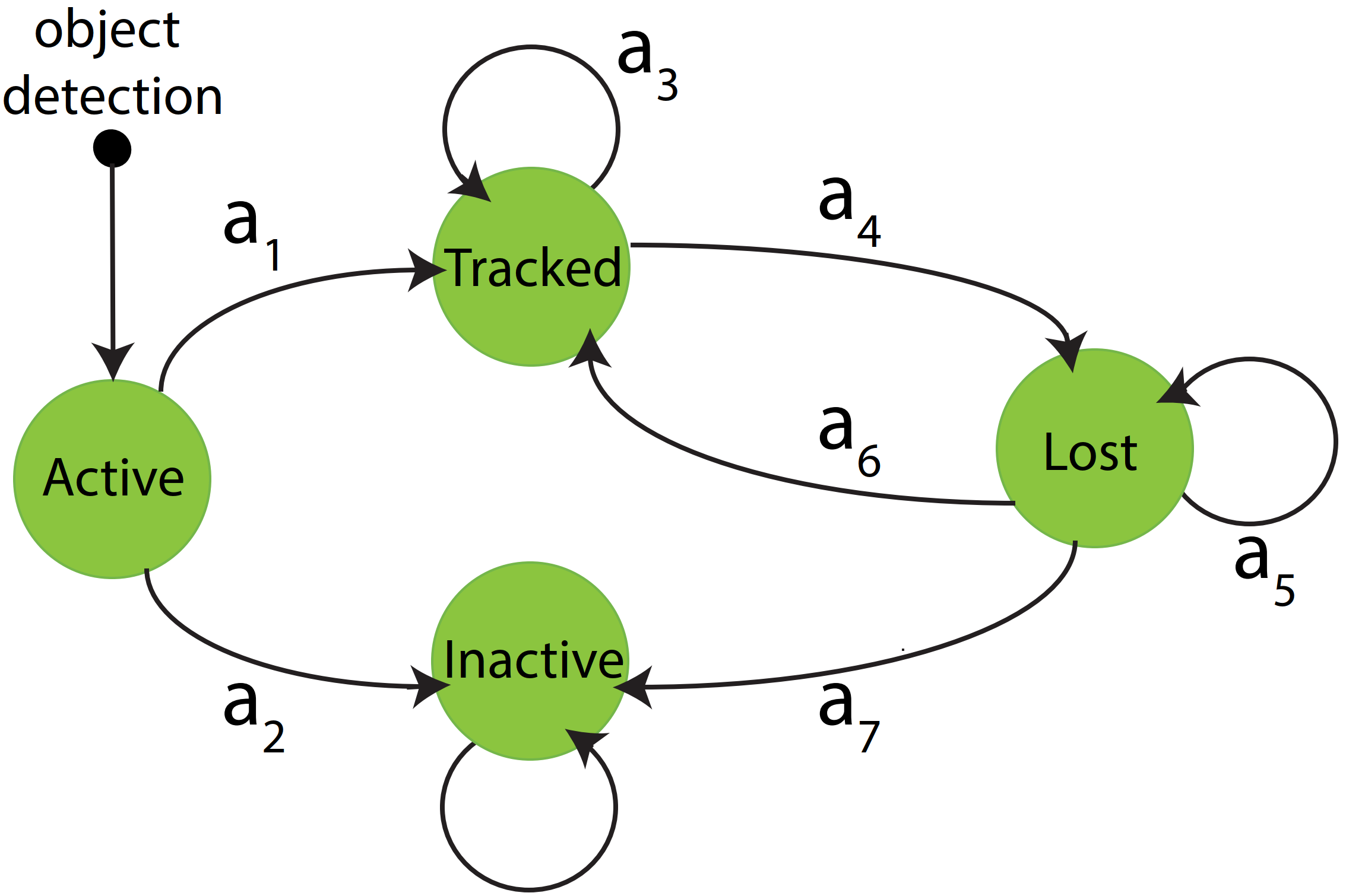
Figure 1: State transition diagram for MDP borrowed from [54]. Active actions $a_{1}$ and $a_{2}$ respectively correspond to TP and FP detections. Tracked actions $a_{3}$ and $a_{4}$ respectively correspond to an object remaining trackable (e.g. clearly visible) and becoming untrackable (e.g. occluded) in the current frame. Lost actions $a_{6}$ and $a_{5}$ are analogous to $a_{3}$ and $a_{4}$ while $a_{7}$ corresponds to an object that has permanently left the scene. Though not shown here or mentioned in the paper, the MDP code also has a transition from tracked to inactive which is made using the same sort of heuristics as $a_{7}$.

II-B Pairwise Tracking of Templates

TABLE I: Impact of the number of templates on tracking performance. Results were generated using original MDP on DETRAC dataset but similar trends hold with deep MDP as well as over other datasets.

no. of templates	higher is better			lower is better
	MOTA (%)	MOTP (%)	MT(%)	ML(%)	IDS
2	84.81	54.84	91.52	2.45	2592
5	84.68	55.98	91.74	2.23	2641
10	84.13	56.17	92.52	1.78	2856

MDP uses tracking more as a way to measure the similarity between two patches representing prospective objects in different frames than to actually track objects over time. Given the object locations in two possibly non-consecutive frames, an ROI centered on the object is extracted from each frame, with a certain amount of its background included for context, and then scaled anisotropically to a fixed size. The default parameters, tuned for tall boxes corresponding to pedestrians, result in an object size of $60\times 45$ with a $120\times 45$ border for an ROI size of $300\times 135$. Forward-backward LK tracking [21] is then applied on the $60\times 45$ boxes between the two ROIs and its success is used as a proxy for how similar the two objects are. This kind of discontinuous ROI-to-ROI tracking works with optical flow methods like LK but it is not suitable for normal long-term trackers.

One of the two ROIs being tracked corresponds to either the predicted location (in tracked) or a detection (in lost), both from the current frame. The other ROI is one of several templates, which are ROIs extracted from heuristically-chosen keyframes from the history of the object. Since each template is tracked independently, this operation not only consumes most of the runtime but also requires additional heuristics to summarize the tracking performance over all the templates in order to generate a single representative feature that can be passed to the classifier. MDP uses a heuristically-selected anchor template to generate this summary feature, thus rendering the expensive template-tracking operation virtually ineffective (Table I). Another heuristic that undermines not only the tracker but the classifier itself is that both tracked and lost policy decisions depend on the presence of a matching detection and it is the latter that gets priority since a missing detection always results in a negative policy decision irrespective of the classification result. All the costly tracking and classification therefore amounts to little more than an additional verification step to confirm that a detection near the expected location of the object actually corresponds to that object.

II-C Training

Training the MDP system involves training the two SVM classifiers for active and lost policies. Active SVM is trained in batch on samples generated by applying two-level thresholding on the intersection-over-union (IOU) of detections with the ground truth (GT) that classifies the former into false positive (FP), true positive (TP) or unknown. FP and TP detections respectively become negative and positive training samples while those classified as unknown are ignored. On the other hand, lost SVM is trained incrementally by tracking one trajectory at a time (Alg. 1) using an untrained or partially trained model for policy decisions, collecting a new sample on each incorrect decision and retraining the model with the new sample added to existing training set. This is a major limitation of this framework not only because trajectory-level training does not allow incorporating inter-target interactions (Alg. 2) that play a major role at inference (Table II) but also with respect to adaptation for deep learning since training deep networks incrementally leads to overfitting and prevents convergence to a good optimum. Another limitation of lost training is that samples can only be extracted from frames where a detection corresponding to the GT is present so that there is no way of learning from FNs.

II-D Modular Implementation

I started by adapting the MATLAB implementation of MDP [53] into a fast, parallelized and modular Python version [45] for real-time vehicle and pedestrian tracking in road traffic videos of intersections captured from pole-mounted and UAV cameras. I also integrated it into an interactive GUI [46] for object detection, MOT and semi-automated labeling. One of my main design objectives was to make it modular so that existing components could be easily swapped with alternatives from deep learning.

There are five main target-level modules in this implementation (Fig. 2) - Templates, History, Lost, Tracked and Active. The latter three correspond to the respective state policies while Templates implements all the functionality that is shared between Tracked and Lost. This includes creating and updating the list of templates representing the object appearance over time, tracking, ROI extraction and heuristics-based feature generation for classification. There are two main global modules - Trainer that trains policies (Alg. 1, Sec. II-C) and Tester that performs inference (Alg. 2). Feature extraction, classification and tracking are also implemented as independent modules but used as submodules within the main modules.

TABLE II: Impact of global heuristics in the original MDP Tester on DETRAC tracking performance. These include target sorting, detection filtering, reconnecting recently lost targets and resolving conflicts between tracked targets. These results also demostrate the inconsistency that often exists between the various MOT metrics in that better performance over some metrics is accompanied by worse performance over others.

config	higher is better			lower is better
	MOTA (%)	MOTP (%)	MT(%)	ML(%)	IDS
heuristics on	84.812	54.844	91.524	2.454	2592
heuristics off	67.629	58.834	97.089	0.960	9435

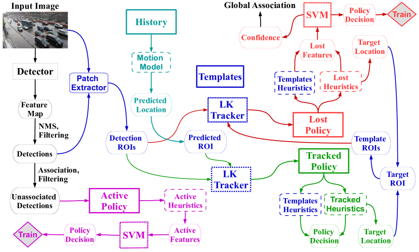
Figure 2: MDP modular implementation block diagrams for (top) target-level and (bottom) global processing. Left: Colors to modules - blue: Templates, cyan: History, red: Lost, green: Tracked, magenta: Active. Lines connecting the various submodules of Templates are not shown for clarity. Right: This shows the inference process for each frame (Alg. 2). Lines connecting association box to targets 1 and 2 are not shown for clarity.

Algorithm 1 MDP Training in Trainer module

1:max_passes, max_trials, max_iters $\leftarrow$ parameters

2:trajectories, detections $\leftarrow$ all trajectories and detections in training set

3:trajectories $\leftarrow$ filterTrajectories(trajectories, detections) $\triangleright$ remove trajectories not suitable for lost training

4:mark all trajectories as trainable

5:pass $\leftarrow$ 0

6:train_samples $\leftarrow$ $\emptyset$

7:for iter $\leftarrow$ 1, max_iters do

8:    mark all trainable trajectories as not done

9:    set trials to 0 for all trajectories

10:    if  all trajectories marked as untrainable  then

11:        break

12:    else if  all trajectories marked as done  then

13:        pass $\leftarrow$ pass + 1

14:        if pass $>$ max_passes then

15:           break         

16:    else

17:        trajectory $\leftarrow$ find the next trajectory marked as not done     

18:    frames $\leftarrow$ all frames in trajectory

19:    failures $\leftarrow$ 0

20:    for each frame $\in$ frames do

21:        dets $\leftarrow$ all detections in frame

22:        success $\leftarrow$ track this object in frame using dets $\triangleright$ success indicates correctness of policy decision

23:        if not success and object is in lost state then

24:           new_sample $\leftarrow$ sample corresponding to incorrect policy decision

25:           train_samples $\leftarrow$ train_samples $\cup$ new_sample

26:           train lost policy with train_samples

27:           failures $\leftarrow$ failures + 1             

28:    if failures $=$ 0 then

29:        mark trajectory as done $\triangleright$ trajectory successfully tracked in entirety

30:    else

31:        increment trajectory trials by 1

32:        if  trajectory trials $>$ max_trials  then

33:           mark trajectory as untrainable $\triangleright$ trajectory is too difficult to track

34:           mark trajectory as done             

35:

36:function filterTrajectories(trajectories, detections)

37:    truncate each trajectory to start in the first frame where:

38:        1. object has at least one detection with IOU $>$ 0.5

39:        2. object does not have IOU $>$ 0 with any other annotation

40:        3. IOU of object with image $>$ 0.95

41:    remove trajectories that have no such frame

Algorithm 2 MDP Inference in Tester module

1:hungarian $\leftarrow$ parameter

2:frames $\leftarrow$ all frames in video

3:trajectories $\leftarrow\emptyset$

4:targets $\leftarrow\emptyset$

5:for each frame $\in$ frames do

6:    dets $\leftarrow$ all detections in frame

7:    sorted $\leftarrow$ sortTargets(targets)

8:    for each target $\in$ sorted do

9:        prev_targets $\leftarrow$ targets processed so far

10:        if target.state = lost then

11:           filtered $\leftarrow$ filterDetections(dets, prev_targets)

12:        else

13:           filtered $\leftarrow$ dets         

14:        track target in frame using filtered

15:        target $\leftarrow$ apply heuristics to check if target left the scene

16:        if target.state = inactive then

17:           trajectories $\leftarrow$ trajectories $\cup$ target.trajectory

18:           targets $\leftarrow$ targets $\setminus$ target         

19:        if  target.state = lost and target.prev_state = tracked  then $\triangleright$ try to reconnect recently lost target

20:           filtered $\leftarrow$ filterDetections(dets, prev_targets)

21:           track target in frame using filtered             

22:    if hungarian then $\triangleright$ otherwise each target associates to highest-probability detection

23:        cost_matrix $\leftarrow$ accumulate classifier probabilities from lost targets

24:        association_matrix $\leftarrow$ HungarianAlgorithm(cost_matrix)

25:        targets $\leftarrow$ associate targets to dets using association_matrix     

26:    unassociated_dets $\leftarrow$ filterDetections(dets, targets)

27:    new_targets $\leftarrow$ apply active policy to unassociated_dets

28:    targets $\leftarrow$ targets $\cup$ new_targets

29:    targets $\leftarrow$ resolveTargetConflicts( targets )

30:trajectories $\leftarrow$ remove trajectories $<$ 5 frames long

31:

32:function sortTargets(targets)

33:    divide targets into two subsets with tracked streaks of $>10$ and $\leq 10$ frames

34:    sort each subset to place tracked targets before lost targets

35:    join the two sorted subsets

36:

37:function filterDetections(detections, targets)

38:    remove detections whose IOU with targets in tracked state exceeds 0.5

39:

40:function resolveTargetConflicts(targets)

41:    find all pairs of tracked targets whose IOU $>$ 0.7

42:    for each pair, remove the one that has shorter tracked streak

43:    if both have identical streak, remove the one having smaller IOU with maximally-overlapping detection

III Deep MDP

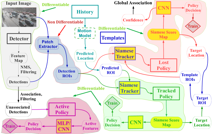
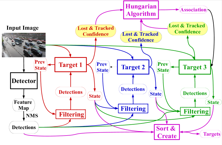
Figure 3: Deep MDP Stage 1 block diagrams for (top) target-level and (bottom) global processing. Changed components with respect to MDP are shown with yellow-filled shapes. (Top) differentiable and non-differentiable parts of the pipeline are highlighted with green and red bordered regions filled with the colours of the respective module.

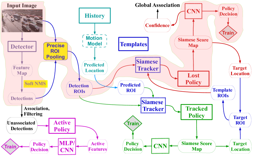
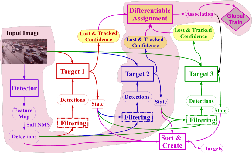
Figure 4: Deep MDP block diagrams for (top) stage 2 target-level and (bottom) stage 3 global processing. Differentiable parts of the pipeline are highlighted with green bordered regions filled with the colour of lost policy. (Top) a differentiable pipeline going through the tracked policy can also be created but not shown for clarity (Bottom) differentiable pipelines going through targets 1 and 3 are not shown for clarity

I started adapting MDP for deep learning with the twin objectives of improving its performance and creating an end-to-end differentiable MOT pipeline. I devised a three stage plan to successively replace non-differentiable components of the framework by differentiable alternatives. In Stage 1 (Fig. 3), I planned to replace the LK tracker with end-to-end differentiable deep learning based trackers [34, 19, 60], heuristics-based features with raw feature maps and SVM with an MLP or CNN classifier. This would be followed in stage 2 (Fig. 4 (top)) by replacing patch extractor with precise ROI pooling [18] to make the ROIs differentiable with respect to detection boxes, thus rendering the target-level pipeline fully differentiable. Also, incorporating soft-NMS [8] would allow signals from all detections to be backpropagated. Finally, I planned in stage 3 (Fig. 4 (bottom)) to replace Hungarian association with a differentiable approximation (Sec. A), thus making the global pipeline end-to-end trainable. I have completed stage 1 implementation but have not succeeded in improving the performance.

The following sections provide brief descriptions for most of the ideas I have tried. Quantitative results from some of these are included too, though it is sufficient to know that none managed to significantly improve performance over the original MDP. Sec. IV also contains details of some of the measures I took to diagnose this poor performance which confirmed that the framework is simply not capable of significant improvement without a complete redesign.

III-A Iterative Batch Training (IBT)

Algorithm 3 Iterative Batch Training

1:max_iters, data_from_tester $\leftarrow$ parameters

2:accumulative_data, train_from_scratch $\leftarrow$ parameters

3:states $\leftarrow$ [active, tracked, lost]

4:training_data $\leftarrow$ $\emptyset$

5:for iter $\leftarrow$ 1, max_iters do

6:    if iter = 1 then

7:        set model to relative oracle for all states

8:    else

9:        set model to neural network for all states

10:        if train_from_scratch then

11:           initialize model weights randomly (or load pretrained weights)

12:        else

13:           load model weights from previous iteration             

14:    if data_from_tester then

15:        new_training_data $\leftarrow$ DataFromTester(states)     

16:    for each state $\in$ states do

17:        if not data_from_tester then

18:           load trained models for previous states from current iteration

19:           new_training_data $\leftarrow$ DataFromTrainer(state)         

20:        if  accumulative_data then

21:           training_data $\leftarrow$ training_data $\cup$ new_training_data

22:        else

23:           training_data $\leftarrow$ new_training_data         

24:        BatchTrain(training_data, state)     

25:    load trained models for all states from current iteration

26:    run Eval() to get classification accuracy on the test set

27:    run Test() to get tracking accuracy on the test set

28:

29:function DataFromTester(states)

30:    enable saving of samples from all policy decisions in all states

31:    run Tester on training set

32:

33:function DataFromTrainer(state)

34:    enable saving of samples from all policy decisions in state

35:    set max_passes and max_trials to 1 so Trainer does a single pass over trajectories

36:    run Trainer on training set

37:

38:function BatchTrain(data, state)

39:    run batch training to train state policy model on data

40:

41:function Eval

42:    enable policy decision evaluation using GT

43:    run Trainer on test set

44:

45:function Test

46:    run Tester on test set

After initial tests confirmed that incremental training would not work for deep networks, I created this new training regime (Alg. 3) to allow for batch training while still retaining several aspects of the original iterative training process (Alg. 1). As its name suggests, IBT involves batch-training of successively better models in an iterative process. Each IBT iteration comprises the following four phases:

1. Data Generation: Run Trainer on the training set to get samples for each state:

   • First iteration: use relative oracle (Sec. IV-D) and save all samples

   • Second iteration onwards: use trained models from the previous iteration and save only incorrectly classified samples

2. Batch Training: Train each state on the samples collected in the data generation phase of the current iteration either by themselves or in addition to the samples collected in previous iterations.

3. Evaluation: Run Trainer on the test set to evaluate classification accuracy

4. Testing: Run Tester on the test set to evaluate tracking performance

Note that the first two phases are run individually for each state while the remaining two are run only once per iteration with the latest trained models loaded for all states.

Data from Tester

I also collected training samples directly by running the Tester to mitigate the aforementioned disconnect between training and inference caused by generating data in the Trainer to train models that are deployed in the Tester. Contrary to standard data generation, this too is run only once per iteration to generate samples jointly for all states.

III-B Tracking

TABLE III: Comparing DETRAC tracking performance with different patch trackers. Siamese-FC, DA-SiamRPN and DiMP were combined with a ResNet18 CNN trained on raw score maps with IBT. LK was combined with SVM and trained using the original Trainer. These results give a good overall idea of the relative performance between MDP and deep MDP.

Tracker	higher is better			lower is better
	MOTA (%)	MOTP (%)	MT(%)	ML(%)	IDS
Siamese-FC	83.508	55.219	79.963	3.035	2902
DA-SiamRPN	78.390	41.389	65.469	5.451	2610
DiMP	84.071	56.006	77.145	3.654	2661
LK	83.708	51.937	76.525	3.561	2233

The first tracker I added was the popular Siamese-FC [5] which failed to outperform LK (Table III) and was also too slow for extensive testing. I followed it with the newer and much faster DA-SiamRPN [63] which I used for a majority of the subsequent testing due to its high speed and relatively low memory requirements. However, this too failed to improve over LK and was in fact slightly worse than Siamese-FC in most cases. I therefore also experimented with several improved Siamese trackers including SiamRPN [28], SiamRPN++ [27], SiamVGG [29] and SiamDW [61] by integrating the SiameseX framework [1] with deep MDP. Finally, I tried several correlation-based trackers including ECO [12], ATOM [13], DiMP [7] and PrDiMP [14] implemented as part of the pytracking [6] framework.

III-B1 Continuous Tracking Mode (CTM)

MDP uses discontinuous ROI-to-ROI tracking (Sec. II-B) that is not suitable for the above trackers since these are designed for continuous long-term tracking. Therefore, I added CTM to the tracked state to bypass the pairwise tracking between templates and predicted locations and instead track an object continuously from the first frame in which it is added. Tracking stops when the object moves from tracked to lost and the tracker is reinitialized when the object transitions back to tracked to account for the frame discontinuity. CTM does improve performance somewhat but not enough to outperform the baseline.

III-C Classification

I first tried using relatively small custom-designed MLPs with 3 to 7 layers for both active and lost policies followed by CNNs with 3 to 8 layers for lost and tracked. These did outperform SVM using handcrafted features from both the original MDP as well as those extracted from the Siamese score maps (sec. III-D) but did not lead to any improvement in the overall MOT performance itself. I then experimented with several off-the shelf networks including VGG-13 [44], MobileNetv2 [41], Inceptionv3 [49], ResNet18/50/101 [17] and ResNext101 [55], though mostly for lost and tracked policies since active policy does not appear to have as much impact on performance. I also modified ResNet to take two image patches as input and process them in parallel through Siamese-style [22] shared layers so that the two ROIs being compared can be fed directly as input without having to go through the tracker.

Model Sharing

Detailed examination of lost and tracked training samples and decision scenarios suggested that both policies require similar discriminative abilities since both need to decide if two patches correspond to the same object. Therefore, I implemented a model sharing functionality where a model trained for one of the policies can also be used for the other.

TABLE IV: Quantitative details of datasets used for evaluation.

Dataset		Subset	Sequences	Frames (K)	Trajectories
Pedestrian	MOT 2015	train	10	5.5	570
		test	10	5.8	721
		total	20	11.3	1291
	MOT 2017	train	7	5.3	796
		test	7	5.9	2354
		total	14	11.2	3150
Vehicle	GRAM	total	3	40.3	751
	IDOT	total	13	111.7	1460
	DETRAC	train	60	83.8	5937
		test	40	56.3	2319
		total	100	140.1	8256
Cell	CTMC	train	47	80.3	1615
		test	39	72	N/A
		total	86	152.3	N/A
	CTC	train	20	8	4299
		test	20	8.1	N/A
		total	40	16.1	N/A

III-D Feature Extraction

Since passing the raw Siamese score maps directly to the classifier works only with CNNs, I also devised a few handcrafted features from these maps for use with MLPs. These are based on the heuristic that successful tracking produces score maps that have a single and relatively concentrated or sharply defined region of maximum. This tends to become more diffused or gets supplemented with additional regions of maxima when the tracking is unsuccessful. The simplest such feature is generated by concatenating the maximum of each row and column in the score map. Another similar way is to concatenate a certain number of the largest values in the score map with optional non-maximum suppression (NMS) to suppress high values in the neighbourhood of each local maximum. A more sophisticated variant involves computing statistics (e.g. mean, median, minmum and maximum) from concetric neighbourhoods of increasing radii around the point of maximum of the score map.

I next used the raw score maps directly as input to the various CNNs I experimented with. Finally, I tried feeding the two image patches themselves as input to Siamese-style ResNet CNNs, thus bypassing the tracker in feature extraction. For feature summarization over templates, I tried taking the elementwise mean of features from all templates as well as concatenating all features into a single multichannel feature fed directly into the classifier in order to learn summarization in the network too.

III-E Class Imbalance

TABLE V: Number of positive and negative training samples collected using IBT data from tester module along with corresponding majority to minority class ratios.

GRAM				DETRAC
policy	negative	positive	ratio	policy	negative	positive	ratio
active	117583	425	276.7	active	28505	287	99.3
tracked	780	44077	56.5	tracked	627	45842	73.1
lost	2553	549	4.7	lost	1865	676	2.8

Significant class imbalance is a major issue in deep MDP training (Table V) that prevents the models from converging to good optima and instead leads to overfitting to a particular class. Following are the main strategies I tested to address this issue:

• Focal loss [30]: Dynamically scale the cross-entropy loss to reduce the weight given to high confidence samples so that training is not overwhelmed by easy to classify examples.

• Online Hard Example Mining (OHEM) [43]: Select a certain ratio of samples with the highest loss and compute the loss using only these so as to concentrate training on the examples that are the most difficult for the network to classify.

• Under sampling: Select a different random subset of the majority class of the same size as the minority class in each epoch

• Over sampling: Randomly duplicate samples from the minority class so that it has the same size as the majority class

• Probabilistic sampling [58]: Draw samples probabilistically from the entire training set such that the probability of each sample being drawn is inversely proportional to its class frequency.

• Synthetic samples: Using each real box as an anchor, generate randomly shifted and resized boxes around it and choose synthetic samples from these by IOU-based thresholding:

  • Negative sample: $0.1<$ IOU with anchor $<0.3$, IOU with other real boxes $<0.3$, IOU with other synthetic boxes $<0.5$

  • Positive sample: $0.5<$ IOU with anchor $<0.8$, IOU with other real boxes $<0.8$, IOU with other synthetic boxes $<0.5$

IV Diagnostics

This section briefly describes some of the many measures I took to diagnose the poor performance of deep MDP along with datasets and metrics I used throughout.

IV-A Datasets

Following are the main datasets I have used:

• Pedestrian: MOT 2015 [24], MOT 2017 [35]

• Vehicle: DETRAC [52], IDOT [20], GRAM [16]

• Cell: CTMC [2], CTC [50]

Table IV provides quantitative details for these.

IV-B Metrics

For most of the testing, I used the CLEAR MOT metrics MOTA and MOTP [4] along with a few other popular metrics from the MOT Challenge [24] including Mostly Tracked (MT), Mostly Lost (ML) and IDS. The inadequacies and mutual inconsistencies of these metrics are well known [26, 36, 3, 39, 25, 32] and it was possible that these could be at least partially responsible for the failure of deep MDP to outperform MDP. Therefore, towards the end, I also experimented with the HOTA metrics [32] that are supposedly less dependent on the detection quality. However, I did not find any significant difference in relative performance of different models between HOTA and the earlier metrics. Following are brief definitions for these metrics:

1. MOTA = $1-\frac{|\text{FN}|+|\text{FP}|+\text{IDS}}{|\text{GT}|}$

2. MOTP: Mean dissimilarity between TPs and their corresponding GTs

3. MT: Fraction of trajectories with $>80\%$ boxes tracked correctly

4. ML: Fraction of trajectories with $<20\%$ boxes tracked correctly

5. IDS: Number of times target ID changes in the middle of its trajectory

6. HOTA: $\sqrt{\text{DetA}\cdot\text{AssA}}$ where

   • $\text{DetA}=\text{Detection Accuracy}=\frac{|\text{TP}|}{|\text{TP}|+|\text{FP}|+|\text{FN}|}$

   • $\text{AssA}=\text{Association Accuracy}=\frac{1}{|\text{TP}|}\sum\limits_{c\in\{\text{TP}\}}\frac{|\text{TPA}|}{|\text{TPA}|+|\text{FPA}|+|\text{FNA}|}$

   • TPA, FPA and FNA are similar to TP, FP and FN except measured at the level of trajectories instead of boxes.

IV-C Validating Benefit of End-to-End Training

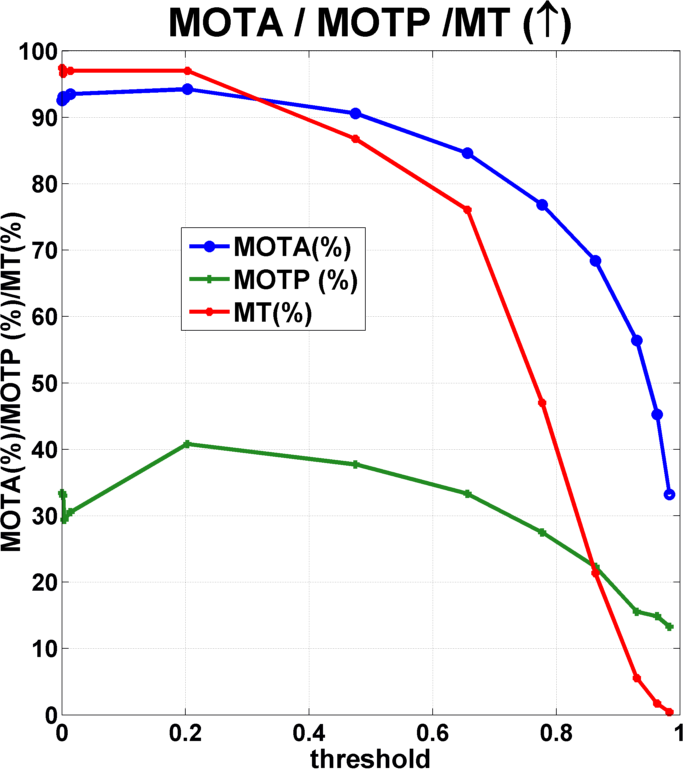
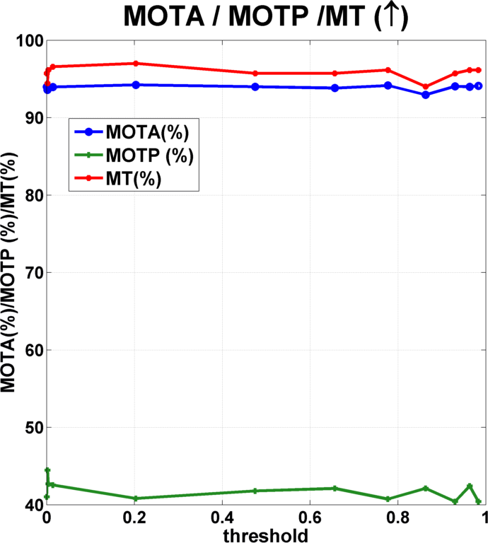
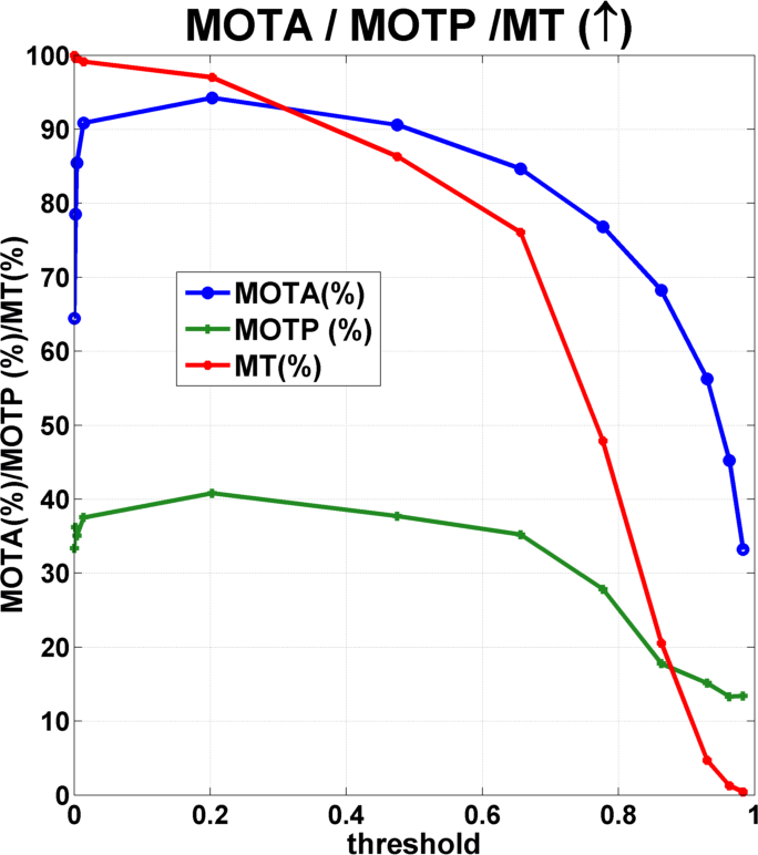
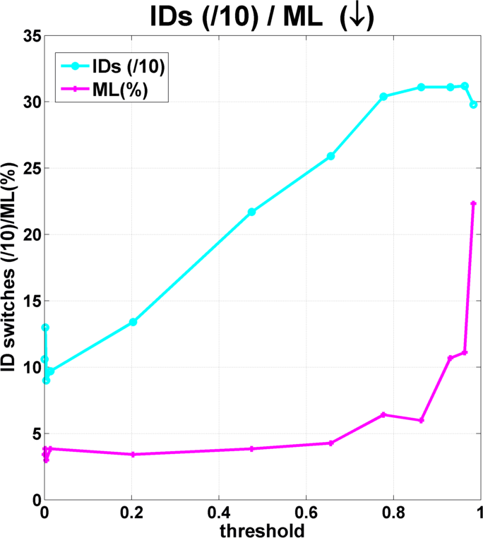
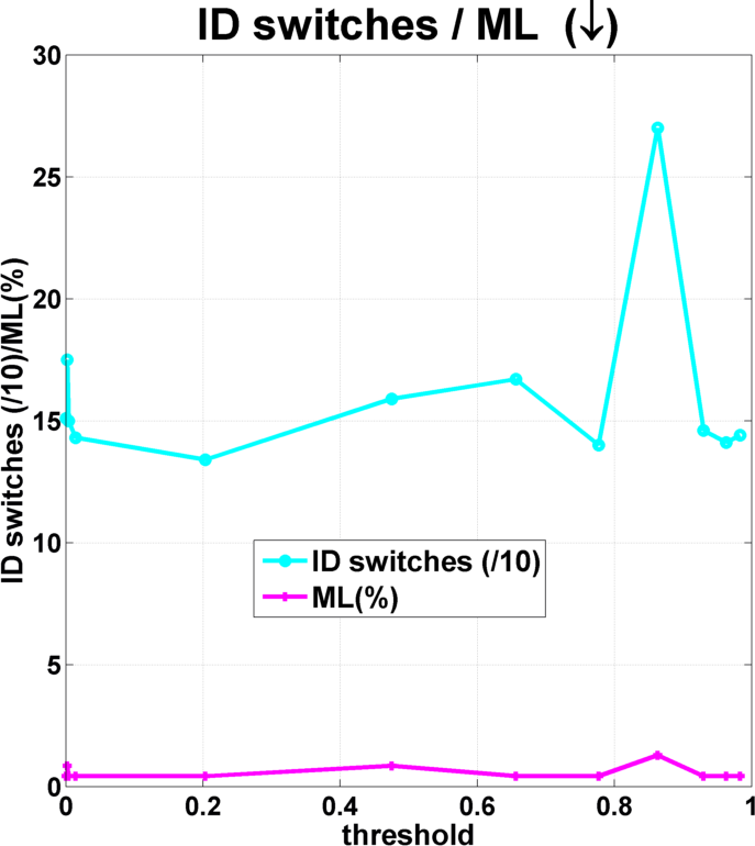
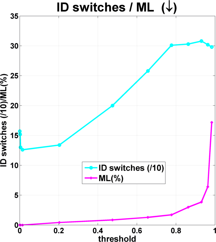
Figure 5: Results of testing three combinations of trackers and detectors with varying recall-precision trade-offs: (from left to right) each tracker with its own detector, all trackers with the best detector and the best tracker with all the detectors. The x-axis in the left and right plots corresponds to detectors with different tradeoffs (obtained by varying the confidence thresholds as shown in Fig. [fig-yolo_rec_prec]) while that in the center plot corresponds to different MDP models trained with these detectors. Top and bottom rows show metrics for which higher and lower is better respectively. IDS(/10) in the latter means that the actual IDS is 10 times the values plotted.
These results were generated using standard MDP with LK and SVM but similar plots were obtained using DA-SiamRPN and DiMP with ResNet18 too so they can be taken to represent module-independent properties of the framework itself. It can be seen that the left and right plots are nearly identical, thus indicating that MDP training process hardly learns anything from the detector and is virtually incapable of adapting itself to the detector characteristics to any degree. The drop in tracking performance with increase in threshold also highlights the well-known fact that MOT performance is far more sensitive to FNs than FPs. Finally, the near-perfect performance of all trackers in the center plot shows the heavy dependence of MDP on detection quality.

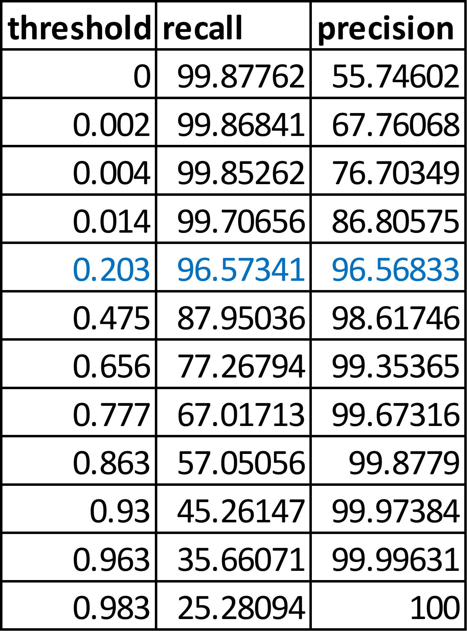
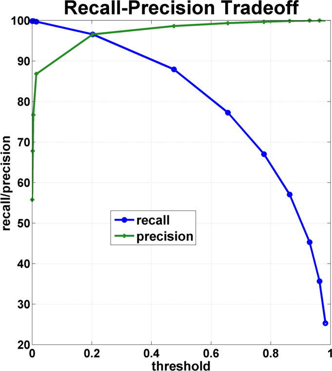
Figure 6: Recall-precision tradeoff for YOLOv3 detector trained on DETRAC. The blue row in the table corresponds to the intersection of recall and precision curves and represents the best detector.

The idea here was to validate the extent to which being able to train the detector to adapt to MDP would improve performance. This can be done by simulating a recall-precision tradeoff for both the detector and MDP and then comparing the performance difference between matched and mismatched combinations of the two. I simulated detection tradeoff by varying the confidence threshold of a YOLOv3 [37] detector trained on DETRAC (Fig. 6). I then trained a new MDP model using each set of detections thus obtained to simulate tracking tradeoff Finally, I performed three-way testing by pairing each tracker with its own detector, all trackers with the best detector, and the best tracker with all the detectors. However, the results of these tests (Fig. 5) showed that MDP learns very little from the detector so that the expedient of training models on detections with different recall-precision characteristics cannot be used to simulate trackers with similar tradeoffs.

IV-D Dummy Policies

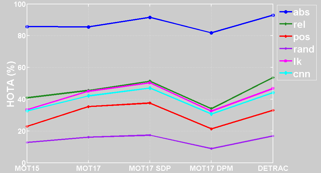
Figure 7: Tracking performance in terms of HOTA for all dummy policies in addition to SVM and CNN on MOT2015, MOT2017 and DETRAC datasets. abs: absolute oracle, rel: relative oracle, pos: positive classifier, rand: random classifier. MOT17, MOT17 SDP and MOT17 DPM respectively refer to results obtained using MOT2017 public detections from Faster-RCNN [38], SDP [57] and DPM [15] detectors.

In order to evaluate the impact of learning better policies on the overall MOT performance, I tested four dummy policies. Two of these are oracles that take the best possible decision given the GT:

• Relative Oracle: This corresponds to how the policies are actually trained and its decisions depend on the detections, tracking result and other policies in addition to the GT. This represents an upper bound for the performance of real policies.

• Absolute Oracle: This is an idealized policy for which no real policy can be trained since it makes decisions using only the GT while ignoring all other cues.

The remaining two policies make decisions independently of any external cues:

• Positive Classifier: This classifies all samples as positive which results in a simplified policy-free MDP where state transitions are governed entirely by presence or absence of detections since active adds all unassociated detections as new targets while tracked and lost always transition to tracked unless a corresponding detection is missing.

• Random Classifier: This classfies each sample randomly

As shown in Fig. 7, relative oracle does indeed perform very similarly to LK and CNN and much worse than absolute oracle which confirms my supposition that training better policies with deep learning is not going to significantly improve the overall tracking performance. I also tried replacing LK with an oracle tracker (similar to oracle policies but for tracking) but that did not yield any useful insights.

IV-E Heuristics

I tried lots of ad-hoc tricks to improve performance, some of which are listed below:

• adding the predicted box from tracked as a pseudo-detection when attempting to reconnect a recently lost target

• removing excessive lost targets by thresholding on the ratio of lost to tracked targets

• improved association method to generate classification GT by matching a detection-GT pair only if the former is the maximum-IOU detection for the latter and the latter is also the maximum-IOU GT for the former

• pre-training active before running IBT iterations for tracked and lost

• ignoring detections in tracked to make policy decision purely with the classifier

V Conclusions

This paper presented a modular library for MOT that was designed to create an end-to-end differentiable pipeline composed of heterogenous and replaceable elements. This goal ultimately proved to be infeasible due to inherent limitations in the MDP framework But the code base that was generated in the process should still be useful to researchers working in this field. The negative results presented in this paper might also help others working on related ideas to avoid wasting time on similar experiments.

Appendix A Differentiable approximations to MOT components

This section includes trackers that approximate a specific part of the MOT pipeline by a differentiable alternative which might in future be useful in constructing a completely differentiable pipeline. All three methods included here have proposed approximations for the association step that is typically performed using the Hungarian algorithm [23] with either handcrafted or learned costs. To the best of my knowledge, this is the only MOT component for which differentiable approximations have so far been proposed.

DAN [47, 48] has introduced one such approximation where the association matrix is directly predicted by limiting the maximum number of detectable objects in each frame to 80 so that the corresponding association matrix has a fixed size of 80 $\times$ 80. Dummy rows and columns containing all zeros are used to fill up the matrix in cases of fewer objects. Two different association matrices of size 81 $\times$ 80 and 80 $\times$ 81 are then constructed by respectively adding an extra row and column to the base matrix These account for objects that disappear or appear in the second frame and carry out both forward and backward association. Though the network that predicts the association matrix using a pairs of frames is trained on the binary association matrices constructed from GT, its output is not directly used to associate objects in the two frames. Instead, heuristics are used to accumulate information from a certain number of past frames to generate a cost matrix for Hungarian association.

FAMNet [10] takes a more ambitious approach to perform global association over an entire batch of frames rather than only frame-pairs through a modified version of the rank 1 tensor approximation (R1TA) framework [42]. This is implemented by a multi-dimensional assignment (MDA) subnet which takes as input object similarities generated by the Siamese-style affinity subnet which in turn takes object-level image features extracted by the feature subnet. Though FAMNet claims to perform global multi-frame association, the basic idea of the R1TA itself involves decomposing the global assignment into a set of local assignments where only pairs of consecutive frames are considered. Practical gains from associating over more than two frames thus remain dubious. In addition, the paper only considers batches of 3 frames which are hardly any improvement over frame pairs anyway. Finally, the process of generating association GT is full of heuristics, as is the formulation of the R1TA power iteration layer in the MDA subnet that has very suboptimal theoretical guarantees.

While the above methods attempt to approximate the binary association matrix that the Hungarian algorithm produces as output, DeepMOT [56] has proposed a Deep Hungarian Net (DHN) module to directly approximate the algorithm itself. DHN uses two bidirectional RNNs to produce a soft approximation to the detection-to-GT assignments. This in turn is used to propose differentiable proxies to the standard MOT metrics of MOTA and MOTP [4] so that the tracker can be optimized directly in terms of these approximate metrics. Unlike DAN [47, 48], DHN is designed to handle variable sized assignment matrices. It takes as input a matrix containing pairwise distances between boxes computed as the average of IOU and normalized Euclidean distances. This matrix is sequentially flattened row-wise and column-wise before being passed through each of the two RNNs to mimic the similar flattening in the Hungarian algorithm. A row and a column containing 0.5 are appended to the soft assignment matrix generated by the DHN to construct two additional matrices which are in turn subjected to column-wise and row-wise softmax respectively followed by summing the extra row and column to finally obtain soft approximations to FP and FN. An approximation to IDS is likewise computed as the L1 norm of the element-wise product between the row-appended matrix above and a binary matrix showing the locations of true positives. The approximate FP, FN and IDS are then used to compute approximate MOTA and MOTP whose weighted average becomes the loss for training the DHN.

References

- [1] SiameseX. online: https://github.com/zllrunning/SiameseX.PyTorch, June 2019.
- [2] S. Anjum and D. Gurari. CTMC: Cell tracking with mitosis detection dataset challenge. CVPR Workshops, pages 4228–4237, 2020.
- [3] J. Bento. A metric for sets of trajectories that is practical and mathematically consistent. ArXiv, abs/1601.03094, 2016.
- [4] K. Bernardin and R. Stiefelhagen. Evaluating multiple object tracking performance: The clear mot metrics. EURASIP Journal on Image and Video Processing, 2008:1–10, 2008.
- [5] L. Bertinetto, J. Valmadre, J. F. Henriques, A. Vedaldi, and P. H. S. Torr. Fully-convolutional siamese networks for object tracking. In ECCV Workshops, 2016.
- [6] G. Bhat. PyTracking. online: https://github.com/visionml/pytracking, April 2022.
- [7] G. Bhat, M. Danelljan, L. V. Gool, and R. Timofte. Learning discriminative model prediction for tracking. ICCV, pages 6181–6190, 2019.
- [8] N. Bodla, B. Singh, R. Chellappa, and L. S. Davis. Soft-NMS — improving object detection with one line of code. ICCV, pages 5562–5570, 2017.
- [9] B. E. Boser, I. Guyon, and V. N. Vapnik. A training algorithm for optimal margin classifiers. In COLT ’92, 1992.
- [10] P. Chu and H. Ling. FAMNet: Joint learning of feature, affinity and multi-dimensional assignment for online multiple object tracking. ICCV, pages 6171–6180, 2019.
- [11] Q. Chu, W. Ouyang, H. Li, X. Wang, B. Liu, and N. Yu. Online multi-object tracking using cnn-based single object tracker with spatial-temporal attention mechanism. ICCV, pages 4846–4855, 2017.
- [12] M. Danelljan, G. Bhat, F. S. Khan, and M. Felsberg. ECO: Efficient convolution operators for tracking. CVPR, pages 6931–6939, 2017.
- [13] M. Danelljan, G. Bhat, F. S. Khan, and M. Felsberg. ATOM: Accurate tracking by overlap maximization. CVPR, pages 4655–4664, 2019.
- [14] M. Danelljan, L. V. Gool, and R. Timofte. Probabilistic regression for visual tracking. CVPR, pages 7181–7190, 2020.
- [15] R. B. Girshick, F. N. Iandola, T. Darrell, and J. Malik. Deformable part models are convolutional neural networks. CVPR, pages 437–446, 2015.
- [16] R. Guerrero-Gómez-Olmedo, R. J. López-Sastre, S. Maldonado-Bascón, and A. Fernández-Caballero. Vehicle tracking by simultaneous detection and viewpoint estimation. In IWINAC, 2013.
- [17] K. He, X. Zhang, S. Ren, and J. Sun. Deep residual learning for image recognition. CVPR, pages 770–778, 2016.
- [18] B. Jiang, R. Luo, J. Mao, T. Xiao, and Y. Jiang. Acquisition of localization confidence for accurate object detection. ECCV, 2018.
- [19] L. Jiao, D. Wang, Y. Bai, P. Chen, and F. Liu. Deep learning in visual tracking: A review. IEEE transactions on neural networks and learning systems, 2021.
- [20] Y. Jin and J. Eriksson. Fully automatic, real-time vehicle tracking for surveillance video. 14th Conference on Computer and Robot Vision (CRV), pages 147–154, 2017.
- [21] Z. Kalal. Tracking-learning-detection. TPAMI, 34:1409–1422, 2012.
- [22] G. R. Koch. Siamese neural networks for one-shot image recognition. ICML, 2015.
- [23] H. W. Kuhn. The hungarian method for the assignment problem. Naval Research Logistics Quarterly, 2:83–97, 1955.
- [24] L. Leal-Taixé, A. Milan, I. Reid, S. Roth, and K. Schindler. MOTChallenge 2015: Towards a benchmark for multi-target tracking. arXiv:1504.01942, Apr. 2015.
- [25] L. Leal-Taixé, A. Milan, K. Schindler, D. Cremers, I. D. Reid, and S. Roth. Tracking the trackers: An analysis of the state of the art in multiple object tracking. ArXiv, abs/1704.02781, 2017.
- [26] I. Leichter and E. Krupka. Monotonicity and error type differentiability in performance measures for target detection and tracking in video. TPAMI, 35 10:2553–60, 2013.
- [27] B. Li, W. Wu, Q. Wang, F. Zhang, J. Xing, and J. Yan. SiamRPN++: Evolution of siamese visual tracking with very deep networks. CVPR, pages 4277–4286, 2019.
- [28] B. Li, J. Yan, W. Wu, Z. Zhu, and X. Hu. High performance visual tracking with siamese region proposal network. CVPR, pages 8971–8980, 2018.
- [29] Y. Li and X. Zhang. SiamVGG: Visual tracking using deeper siamese networks. ArXiv, abs/1902.02804, 2019.
- [30] T.-Y. Lin, P. Goyal, R. B. Girshick, K. He, and P. Dollár. Focal loss for dense object detection. ICCV, pages 2999–3007, 2017.
- [31] L. Liu, W. Ouyang, X. Wang, P. Fieguth, J. Chen, X. Liu, and M. Pietikäinen. Deep learning for generic object detection: A survey. IJCV, 128(2):261–318, 2020.
- [32] J. Luiten, A. Osep, P. Dendorfer, P. H. S. Torr, A. Geiger, L. Leal-Taixé, and B. Leibe. HOTA: A higher order metric for evaluating multi-object tracking. IJCV, 129:548 – 578, 2021.
- [33] W. Luo, X. Zhao, and T. Kim. Multiple object tracking: A review. ArXiv, abs/1409.7618v4, 2017.
- [34] S. M. Marvasti-Zadeh, L. Cheng, H. Ghanei-Yakhdan, and S. Kasaei. Deep learning for visual tracking: A comprehensive survey. IEEE Transactions on Intelligent Transportation Systems, pages 1–26, 2021.
- [35] A. Milan, L. Leal-Taixé, I. Reid, S. Roth, and K. Schindler. MOT16: A benchmark for multi-object tracking. arXiv:1603.00831, Mar. 2016.
- [36] A. Milan, K. Schindler, and S. Roth. Challenges of ground truth evaluation of multi-target tracking. CVPR Workshops, pages 735–742, 2013.
- [37] J. Redmon and A. Farhadi. Yolov3: An incremental improvement. ArXiv, abs/1804.02767, 2018.
- [38] S. Ren, K. He, R. B. Girshick, and J. Sun. Faster R-CNN: Towards real-time object detection with region proposal networks. TPAMI, 39:1137–1149, 2015.
- [39] E. Ristani, F. Solera, R. S. Zou, R. Cucchiara, and C. Tomasi. Performance measures and a data set for multi-target, multi-camera tracking. ECCV Workshops, 2016.
- [40] A. Sadeghian, A. Alahi, and S. Savarese. Tracking the untrackable: Learning to track multiple cues with long-term dependencies. ICCV, pages 300–311, 2017.
- [41] M. Sandler, A. G. Howard, M. Zhu, A. Zhmoginov, and L.-C. Chen. Mobilenetv2: Inverted residuals and linear bottlenecks. CVPR, pages 4510–4520, 2018.
- [42] X. Shi, H. Ling, Y. Pang, W. Hu, P. Chu, and J. Xing. Rank-1 tensor approximation for high-order association in multi-target tracking. IJCV, 2019.
- [43] A. Shrivastava, A. K. Gupta, and R. B. Girshick. Training region-based object detectors with online hard example mining. CVPR, pages 761–769, 2016.
- [44] K. Simonyan and A. Zisserman. Very deep convolutional networks for large-scale image recognition. ICLR, 2015.
- [45] A. Singh. Deep MDP. online: https://github.com/abhineet123/deep_mdp, April 2022.
- [46] A. Singh. MDP Labeling Tool. online: https://github.com/abhineet123/mdp_labeling_tool, April 2022.
- [47] S. Sun, N. Akhtar, H. Song, A. S. Mian, and M. Shah. Deep affinity network for multiple object tracking. ArXiv, arXiv:1810.11780, 2018.
- [48] S. Sun, N. Akhtar, H. Song, A. S. Mian, and M. Shah. Deep affinity network for multiple object tracking. TPAMI, 43:104–119, 2021.
- [49] C. Szegedy, V. Vanhoucke, S. Ioffe, J. Shlens, and Z. Wojna. Rethinking the inception architecture for computer vision. CVPR, pages 2818–2826, 2016.
- [50] V. Ulman, M. Mavska, K. E. G. Magnusson, O. Ronneberger, C. Haubold, N. Harder, P. Matula, P. Matula, D. Svoboda, M. Radojević, I. Smal, K. Rohr, J. Jaldén, H. M. Blau, O. Dzyubachyk, B. P. F. Lelieveldt, P. Xiao, Y. Li, S.-Y. Cho, A. C. Dufour, J.-C. Olivo-Marin, C. C. Reyes-Aldasoro, J. A. Solís-Lemus, R. Bensch, T. Brox, J. Stegmaier, R. Mikut, S. Wolf, F. A. Hamprecht, T. Esteves, P. Quelhas, Ö. Demirel, L. Malmström, F. Jug, P. Tomançak, E. H. W. Meijering, A. Muñoz-Barrutia, M. Kozubek, and C. O. de Solórzano. An objective comparison of cell tracking algorithms. Nature methods, 14:1141 – 1152, 2017.
- [51] X. Wan, J. Cao, S. Zhou, J. Wang, and N. Zheng. Tracking beyond detection: Learning a global response map for end-to-end multi-object tracking. TIP, 30:8222–8235, 2021.
- [52] L. Wen, D. Du, Z. Cai, Z. Lei, M.-C. Chang, H. Qi, J. Lim, M.-H. Yang, and S. Lyu. UA-DETRAC: A new benchmark and protocol for multi-object detection and tracking. CVIU, 193:102907, 2020.
- [53] Y. Xiang. MDP Tracking. online: https://github.com/yuxng/MDP_Tracking, March 2017.
- [54] Y. Xiang, A. Alahi, and S. Savarese. Learning to track: Online multi-object tracking by decision making. ICCV, pages 4705–4713, 2015.
- [55] S. Xie, R. B. Girshick, P. Dollár, Z. Tu, and K. He. Aggregated residual transformations for deep neural networks. CVPR, pages 5987–5995, 2017.
- [56] Y. Xu, A. Osep, Y. Ban, R. Horaud, L. Leal-Taixé, and X. Alameda-Pineda. How to train your deep multi-object tracker. CVPR, pages 6786–6795, 2020.
- [57] F. Yang, W. Choi, and Y. Lin. Exploit all the layers: Fast and accurate cnn object detector with scale dependent pooling and cascaded rejection classifiers. CVPR, pages 2129–2137, 2016.
- [58] M. Yang. Imbalanced Dataset Sampler. online: https://github.com/ufoym/imbalanced-dataset-sampler, January 2022.
- [59] J. yves Bouguet. Pyramidal implementation of the lucas kanade feature tracker. In Intel Corporation, Microprocessor Research Labs, 2001.
- [60] X. Zhang, R. Jiang, C. Fan, T.-Y. Tong, T. Wang, and P. Huang. Advances in deep learning methods for visual tracking: Literature review and fundamentals. Int. J. Autom. Comput., 18:311–333, 2021.
- [61] Z. Zhang, H. Peng, and Q. Wang. Deeper and wider siamese networks for real-time visual tracking. CVPR, pages 4586–4595, 2019.
- [62] J. Zhu, H. Yang, N. Liu, M. Kim, W. Zhang, and M.-H. Yang. Online multi-object tracking with dual matching attention networks. In ECCV, 2018.
- [63] Z. Zhu, Q. Wang, B. Li, W. Wu, J. Yan, and W. Hu. Distractor-aware siamese networks for visual object tracking. In ECCV, 2018.