Data-driven Morozov regularization of inverse problems

Abstract

The solution of inverse problems is central to a wide range of applications including medicine, biology, and engineering. These problems require finding a desired solution in the presence of noisy observations. A key feature of inverse problems is their ill-posedness, which leads to unstable behavior under noise when standard solution methods are used. For this reason, regularization methods have been developed that compromise between data fitting and prior structure. Recently, data-driven variational regularization methods have been introduced, where the prior in the form of a regularizer is derived from provided ground truth data. However, these methods have mainly been analyzed for Tikhonov regularization, referred to as Network Tikhonov Regularization (NETT). In this paper, we propose and analyze Morozov regularization in combination with a learned regularizer. The regularizers, which can be adapted to the training data, are defined by neural networks and are therefore non-convex. We give a convergence analysis in the non-convex setting allowing noise-dependent regularizers, and propose a possible training strategy. We present numerical results for attenuation correction in the context of photoacoustic tomography.

Key words: Inverse problems, learned regularizer, convergence analysis, Morozov regularization.

MSC codes: 65F22; 68T07

1 Introduction

In this paper, we consider the solution of linear inverse problems where we aim to reconstruct the unknown $x\in\mathbb{X}$ from noisy data

$$y_{\delta}=\mathbf{A}x+\eta_{\delta}\,.$$ (1.1)

Here $\mathbf{A}\colon\mathbb{X}\to\mathbb{Y}$ is a linear bounded operator between Hilbert spaces $\mathbb{X}$ and $\mathbb{Y}$, and $\eta_{\delta}$ is the data error that satisfies $\lVert\eta_{\delta}\rVert\leq\delta$ with noise level $\delta\geq 0$. We are especially interested in the ill-posed case where solving (1.1) without prior information is non-unique or unstable. Several applications in medical image reconstruction, nondestructive testing, and remote sensing are instances of such linear inverse problems [9, 23, 28].

Characteristic features of inverse problems are the non-uniqueness of solutions and the unstable dependence of solutions on data perturbations. To account for these two issues, one must apply regularization methods (see, for example, [15, 9, 28, 4, 14, 29, 16, 21, 31]) that serve two main purposes: First, in the case of exact data $y\in\operatorname{ran}(\mathbf{A})$, they select a specific solution $\mathbf{B}_{0}(y)$ among all possible solutions of the exact data equation $y=\mathbf{A}x$. Second, to account for noise, they define stable approximations to $\mathbf{B}_{0}$ in the form of continuous mappings $\mathbf{B}_{\alpha}\colon\mathbb{Y}\to\mathbb{X}$ that converge to $\mathbf{B}_{0}$ as $\alpha\to 0$ in an appropriate sense.

1.1 Morozov regularization

There are several well established methods for the stable solution of inverse problems. A general class of regularization methods are variational regularization methods which includes Tikhhonov regularization, Ivanov regularization (the method of quasi solutions), and Morozov regularization (the residual method) as special cases. In Tikhonov regularization, approximate solutions are defined as minimizers of $\lVert\mathbf{A}x-y_{\delta}\rVert^{2}/2+\alpha\mathcal{R}(x)$, where $\mathcal{R}\colon\mathbb{X}\to[0,\infty]$ is a regularization functional that measures the feasibility of a potential solution and $\alpha$ is the regularization parameter. Ivanov regularization considers minimizers of $\lVert\mathbf{A}x-y_{\delta}\rVert$ over the set $\{x\in\mathbb{X}\mid\mathcal{R}(x)\leq\tau\}$ for some $\tau>0$. In this paper, we consider Morozov regularization where approximate solutions defined as solutions of

$$\min_{x\in\mathbb{X}}\mathcal{R}(x)\quad\text{s.t. }\quad\lVert\mathbf{A}x-y_{\delta}\rVert\leq\delta\,.$$ (1.2)

Compared to Tikhonov regularization and Ivanov regularization, the latter has the advantage that no additional regularization parameter has to be selected, which is typically a difficult issue. Relations between Tikhonov regularization, Ivanov regularization and Morozov regularization are carefully studied in [16].

Note that variational regularization methods are designed to approximate $\mathcal{R}$-minimizing solution of $\mathbf{A}x=y$ for the limit $\delta\to 0$, defined as elements in $\operatorname*{arg\,min}\{\mathcal{R}(x)\mid\mathbf{A}x=y\}$. This addresses the non-uniqueness in the case of exact data. To account for noise, Morozov regularization relaxes the strict data consistency $\mathbf{A}x=y$ to data proximity $\lVert\mathbf{A}x-y_{\delta}\rVert\leq\delta$. Even in the case that $\mathbf{A}$ is injective, different regularization terms behave differently and significantly affect convergence. Therefore the choice of the regularizer is crucial and a nontrivial issue. Classical choices for the regularizers are the squared Hilbert space norm $\mathcal{R}(x)=\lVert x\rVert^{2}/2$ or the $\ell^{1}$-norm $\mathcal{R}(x)=\sum_{\lambda\in\Lambda}\lvert\langle u_{\lambda},x\rangle\rvert$, where $(u_{\lambda})_{\lambda}$ is a frame of $\mathbb{X}$. These regularizers may not be optimally adapted to highly structured signal classes, as is often the case in practical applications. In this paper, we address this issue and propose a data-driven regularizer using neural networks adapted to the signal class represented by training data in combination with Morozov regularization.

1.2 Neural network regularizers

In this paper, we study Morozov regularization with a Neural network based and data-driven and noise-dependent regularizer

$$\mathcal{R}_{\delta}(x)=\frac{1}{2}\lVert\boldsymbol{\Phi}_{\theta(\delta)}(x)-x\rVert^{2}+\lambda\,\mathcal{Q}(x)\,.$$ (1.3)

Here $\boldsymbol{\Phi}_{\theta(\delta)}\colon\mathbb{X}\to\mathbb{X}$ is a neural network tuned to noisy data, and $\mathcal{Q}\colon\mathbb{X}\to[0,\infty]$ is an additional noise-adaptive data-driven regularization term. We will refer to (1.2) with the data-driven regularizer (1.3) instead of the fixed regularizer $\mathcal{R}$ as data-driven Morozov (DD-Morozov) regularization and show that, under reasonable assumptions, this gives a regularization method. Furthermore, we present a training strategy for selecting the noise-dependent neural network among a given architecture.

Besides stabilizing the signal reconstruction, the main purpose of a particular regularizer is to fit the reconstructions to a certain set where the true signals are likely to be contained. In reality, this set is not known analytically, but it is possible to draw examples from it. For this reason, we follow the learning paradigm and choose training signals $x_{1},\dots,x_{N}\in\mathbb{X}$ and adapt the architecture $(\boldsymbol{\Phi}_{\theta})_{\theta\in\theta}$ to $x_{i}$. More precisely, $\theta=\theta(\delta)$ is chosen such that $\boldsymbol{\Phi}_{\theta}(x_{i})\simeq x_{i}$ and $\boldsymbol{\Phi}_{\theta}(x_{i}+r_{i,j})\simeq x_{i}$, where $r_{i,j}$ are appropriate perturbations. Thus, $\mathcal{R}_{\delta}$ has small values for the exact $x_{i}$ and larger values for the perturbed signals $x_{i}+r_{i,j}$. Since the training data is only taken from a certain subset of $\mathbb{X}$, it is difficult to obtain the necessary coercive condition from training alone. Therefore, it seems natural to add another regularization term $\mathcal{Q}$ which is known to be coercive.

While learned regularizers have recently become popular in the context of Tikhonov regularization [19, 24, 20, 11], we are not aware of any work utilizing the Morozov variant. In fact, our analysis as well as the training strategy are closely related to the Network Tikhonov Approach (NETT) of [19, 24]. However, in this paper we use a refined training strategy that is suitable for ill-posed problems and we consider a different regularization concept. A different strategy for learning a network regularizer has been proposed in [20] in the context of adversarial regularization. Other approaches for learning a regularizer are the fields of experts model [27], deep total variation [17] or ridge regularizers [11]. Other data-driven regularization methods for inverse problems can be found for example in [1, 3, 2, 14, 22, 25, 30, 7] and the references therein. From the theoretical side, Morozov regularization in a general non-convex context has been studied in [12]. The analysis we present below allows the regularizer to be noise-dependent and further we derive strong convergence under total nonlinearity condition of [19].

1.3 Outline

The remainder of this paper is organized as follows. In Section 2 we present our theoretical results. In particular we present the convergence analysis (Section 2.1) and the prosed training strategy (Section 2.2). In Section 3 we present numerical results illustrating our proposal. Specifically, we test our reconstruction strategy on a severely ill-posed problem regarding attenuation correction for photoacoustic tomography in damping media [18]. To numerically solve (1.2) we implement the primal dual scheme of [6]. The paper concludes with a short summary in Section 4 .

2 Theory

Throughout this paper, $\mathbb{X}$, $\mathbb{Y}$ are Hilbert spaces and $\mathbf{A}\colon\mathbb{X}\to\mathbb{Y}$ a bounded linear operator. Recall that a functional $\mathcal{R}\colon\mathbb{X}\to[0,\infty]$ is coercive, if $\mathcal{R}(x_{n})\to\infty$ for all sequences $(x_{n})_{n\in\mathds{N}}\in\mathbb{X}^{\mathds{N}}$ with $\|x_{n}\|_{\mathbb{X}}\to\infty$, and weakly lower semicontinuous, if $\mathcal{R}(x)\leq\liminf_{n\to\infty}\mathcal{R}(x_{n})$ for $(x_{n})_{n\in\mathds{N}}\rightharpoonup x$, where $\rightharpoonup$ denotes weak convergence, and $\to$ strong convergence. Any element in $\operatorname*{arg\,min}{\left\{\mathcal{R}(x)\mid\mathbf{A}x=y\right\}}$ is called an $\mathcal{R}$-minimizing solution of the equation $\mathbf{A}x=y$.

2.1 Convergence analysis

For networks $\boldsymbol{\Phi},\boldsymbol{\Phi}_{\theta(\delta)}$ on $\mathbb{X}$ and $\delta>0$ we define the noise-dependent regularizer $\mathcal{R}_{\delta}$ by (1.3), the limiting regularizer by $\mathcal{R}(x)=\lVert\boldsymbol{\Phi}(x)-x\rVert^{2}/2+\lambda\,\mathcal{Q}(x)$ and consider noise-adaptive DD-Morozov regularization

$$\min_{x\in\mathbb{X}}\mathcal{R}_{\delta}(x)\quad\text{s.t. }\quad\lVert\mathbf{A}x-y_{\delta}\rVert\leq\delta\,.$$ (2.1)

Our results on the convergence of (1.3), (2.1) are derived under the following conditions, which we assume to be satisfied throughout this subsection.

Assumption 2.1.

1. $\boldsymbol{\Phi},\boldsymbol{\Phi}_{\theta(\delta)}\colon\mathbb{X}\to\mathbb{X}$ are weakly continuous.

2. $\boldsymbol{\Phi}_{\theta(\delta)}\to\boldsymbol{\Phi}$ weakly uniformly on bounded sets as $\delta\to 0$.

3. $\boldsymbol{\Phi}_{\theta(\delta)}\to\boldsymbol{\Phi}$ strongly pointwise on $\mathcal{R}$-minimizing solutions as $\delta\to 0$.

4. $\mathcal{Q}\colon\mathbb{X}\to[0,\infty]$ is proper, coercive and weakly lower semicontinuous.

In (A2), weak uniform convergence on bounded sets means that for all bounded $B\subseteq\mathbb{X}$ and all $h\in\mathbb{X}$ we have $\sup_{x\in B}\lvert\langle\boldsymbol{\Phi}_{\theta(\delta)}(x)-\boldsymbol{\Phi}(x),h\rangle\rvert=0$ as $\delta\to 0$. In the convergence analysis we assume that the networks $\boldsymbol{\Phi}_{\theta(\delta)}$ are trained, where $\theta(\delta)$ potentially depends on the noise, and all other quantities are given by the application or are user-specified. In many applications, the function $\boldsymbol{\Phi}_{\theta(\delta)}$ is a neural network for which $\lVert(\boldsymbol{\Phi}_{\theta(\delta)}-\operatorname{Id})(\cdot)\rVert$ may not be coercive which is the reason to add the term $\mathcal{Q}$ in (1.3).

Lemma 2.2.

The regularizers $\mathcal{R},\mathcal{R}_{\delta}$ are coercive and weakly sequentially lower semicontinuous. Further, the feasible set $\{x\in\mathbb{X}\mid\lVert\mathbf{A}x-y_{\delta}\rVert\leq\delta\}$ is weakly closed and non-empty for all $\delta>0$ and all data $y_{\delta}$ with $\lVert\mathbf{A}x_{\star}-y_{\delta}\rVert\leq\delta$ for some $x_{\star}\in\operatorname{dom}(\mathcal{Q})$.

Proof.

Let $(x_{n})_{n\in\mathds{N}}\in\mathbb{X}^{\mathds{N}}$. Because $\mathcal{Q}$ is coercive and $\lVert\boldsymbol{\Phi}_{\theta(\delta)}(x)-x\rVert^{2}$ and $\lVert\boldsymbol{\Phi}(x)-x\rVert^{2}$ are non-negative, the functionals $\mathcal{R},\mathcal{R}_{\delta}$ are coercive. Let $(x_{n})_{n\in\mathds{N}}\in\mathbb{X}^{\mathds{N}}$ converge weakly to $x\in\mathbb{X}$. Because $\boldsymbol{\Phi}$ is weakly continuous, $(\boldsymbol{\Phi}(x_{n})-x_{n})_{n\in\mathds{N}}$ converges weakly to $\boldsymbol{\Phi}(x)-x$. Due to the weak sequential lower semicontinuity of the norm, we infer $\|\boldsymbol{\Phi}(x)-x\|_{\mathbb{X}}\leq\liminf_{n\to\infty}\|\boldsymbol{\Phi}(x_{n})-x_{n}\|_{\mathbb{X}}$ which shows that $\mathcal{R}$ and in a similar manner $\mathcal{R}_{\delta}$ are weakly lower semicontinuous. Now, according to [5, Lemma 1.2.3], a functional $\mathcal{F}$ is weakly sequentially lower semicountinuous if and only if $\{x\in\mathbb{X}\mid\mathcal{F}(x)\leq t\}$ is weakly sequentially closed for all $t>0$. Because $\mathbf{A}$ is linear and bounded it is weakly continuous. Because the norm is weakly sequentially lower semicontinuous, $x\mapsto\lVert\mathbf{A}x-y_{\delta}\rVert$ is weakly sequentially lower semicontinuous, too. Hence $\{x\in\mathbb{X}\mid\lVert\mathbf{A}x-y_{\delta}\rVert\leq\delta\}$ is weakly closed for all $\delta>0$ and non-empty as it contains the exact data $\mathbf{A}x_{\star}$. ∎

Lemma 2.3 (Existence).

For all data $y_{\delta}\in\mathbb{Y}$ with $\lVert\mathbf{A}x_{\star}-y_{\delta}\rVert\leq\delta$ for some $x_{\star}\in\operatorname{dom}(\mathcal{Q})$, the constraint optimization problem (2.1) has at least one solution.

Proof.

Because $\mathcal{R}_{\delta}\geq 0$, the infimum $M$ of $\mathcal{R}$ over $S_{\delta}\coloneqq\{x\in\mathbb{X}\mid\lVert\mathbf{A}x-y_{\delta}\rVert\leq\delta\}$ is nonnegative and there exists a sequence $(x_{m})_{m}$ of elements of $S_{\delta}$ with $\lim_{m\to\infty}\mathcal{R}_{\delta}(x_{m})=M$. Because $\mathcal{R}_{\delta}$ is coercive and $\{\mathcal{R}_{\delta}(x_{m})\,|\,m\in\mathds{N}\}$ is bounded, we infer that $(x_{m})_{m}$ is bounded and thus there exists a weakly convergent subsequence $(x_{m(k)})_{k}$ converging to some $x\in\mathbb{X}$. Moreover, due to the weak closedness of $S_{\delta}$ we obtain $x\in S_{\delta}$. Because $\mathcal{R}_{\delta}$ is weakly lower semicontinuous, $\mathcal{R}(x)\leq M$ and thus $x$ is a solution of (1.2). ∎

Analogous to the proof of Lemma 2.3 one shows that there exists at least one $\mathcal{R}$-minimizing solution of $\mathbf{A}x=y$ whenever it is solvable in $\operatorname{dom}(\mathcal{Q})$.

Theorem 2.4 (Weak convergence).

Let $\mathbf{A}x=y$ be solvable in $\operatorname{dom}(\mathcal{Q})$, $(y_{n})_{n\in\mathds{N}}\in\mathbb{Y}^{\mathds{N}}$ satisfy $\lVert y-y_{n}\rVert\leq\delta_{n}$, where $(\delta_{n})_{n\in\mathds{N}}\in(0,\infty)^{\mathds{N}}$ with $\delta_{n}\to 0$, write $\mathcal{R}_{n}\coloneqq\mathcal{R}_{\delta_{n}}$ and $\boldsymbol{\Phi}_{n}\coloneqq\boldsymbol{\Phi}_{\theta(\delta_{n})}$, and choose $x_{n}\in\operatorname*{arg\,min}\{\mathcal{R}_{n}(z)\mid\lVert\mathbf{A}z-y_{n}\rVert\leq\delta_{n}\}$. Then $(x_{n})_{n\in\mathds{N}}$ has at least one weak accumulation point $x^{\boldsymbol{\texttt{+}}}\in\mathbb{X}$. Moreover, the limit of each weakly converging subsequence $(x_{n(k)})_{k\in\mathds{N}}$ is an $\mathcal{R}$-minimizing solution of $\mathbf{A}x=y$ and $\mathcal{R}_{n(k)}(x_{n(k)})\to\mathcal{R}(x^{\boldsymbol{\texttt{+}}})$ for $k\to\infty$. If the $\mathcal{R}$-minimizing solution $x^{\boldsymbol{\texttt{+}}}$ of $\mathbf{A}x=y$ is unique, then $x_{n}\rightharpoonup x^{\boldsymbol{\texttt{+}}}$ and $\mathcal{R}_{n}(x_{n})\to\mathcal{R}(x^{\boldsymbol{\texttt{+}}})$ as $n\to\infty$.

Proof.

Set $S_{n}\coloneqq\{z\in\mathbb{X}\mid\lVert\mathbf{A}z-y_{n}\rVert\leq\delta_{n}\}$ and $S_{\star}\coloneqq\{z\in\mathbb{X}\mid\mathbf{A}z=y\}$. Clearly $S_{\star}\subseteq S_{n}$ and because $\mathbf{A}x=y$ is solvable, $S_{\star}$ is non-empty. Thus $\mathcal{R}_{n}(x_{n})\leq\mathcal{R}_{n}(x^{\boldsymbol{\texttt{+}}})=\mathcal{Q}(x^{\boldsymbol{\texttt{+}}})+\lVert\boldsymbol{\Phi}_{n}(x_{\star})-x_{\star}\rVert^{2}/2$, where $x_{\star}$ is an $\mathcal{R}$-minimizing solution of $\mathbf{A}x=y$. From the weak convergence of $\boldsymbol{\Phi}_{n}(x_{\star})$ we see that the right hand side is bounded. Thus $\mathcal{Q}(x_{n})$ is bounded and with the coercivity of $\mathcal{Q}$ we conclude there exists a weakly converging subsequence $(x_{n(k)})_{k\in\mathds{N}}$. Because $\|\mathbf{A}(\cdot)-y\|$ is weakly lower semicontinuous,

$$\|\mathbf{A}(x^{\boldsymbol{\texttt{+}}})-y\|\leq\liminf_{k\to\infty}\|\mathbf{A}(x_{n(k)})-y\|\\ \leq\liminf_{k\to\infty}\|\mathbf{A}(x_{n(k)})-y_{n(k)}\|+\|y_{n(k)}-y\|\leq 2\delta_{n}$$ (2.2)

and thus $x^{\boldsymbol{\texttt{+}}}\in S_{\star}$. It remains to verify that $x^{\boldsymbol{\texttt{+}}}$ is an $\mathcal{R}$-minimizing solution of $\mathbf{A}x=y$. According to (A1), (A2) we have $\boldsymbol{\Phi}_{n(k)}(x_{n(k)})\rightharpoonup\boldsymbol{\Phi}(x^{\boldsymbol{\texttt{+}}})$ and $\boldsymbol{\Phi}_{n}(x_{\star})\to\boldsymbol{\Phi}(x_{\star})$, and thus

$$\mathcal{Q}(x^{\boldsymbol{\texttt{+}}})+\frac{\lambda}{2}\lVert\boldsymbol{\Phi}(x^{\boldsymbol{\texttt{+}}})-x^{\boldsymbol{\texttt{+}}}\rVert \leq\liminf_{n\to\infty}\mathcal{Q}(x_{n})+\frac{\lambda}{2}\lVert\boldsymbol{\Phi}_{n}(x_{n})-x_{n}\rVert$$

$$\leq\limsup_{n\to\infty}\mathcal{Q}(x_{n})+\frac{\lambda}{2}\lVert\boldsymbol{\Phi}_{n}(x_{n})-x_{n}\rVert$$

$$\leq\limsup_{n\to\infty}\mathcal{Q}(x_{\star})+\frac{\lambda}{2}\lVert\boldsymbol{\Phi}_{n}(x_{\star})-x_{\star}\rVert$$

$$=\mathcal{Q}(x_{\star})+\frac{\lambda}{2}\lVert\boldsymbol{\Phi}(x_{\star})-x_{\star}\rVert\,.$$

Thus $x^{\boldsymbol{\texttt{+}}}$ is an $\mathcal{R}$-minimizing solution of $\mathbf{A}x=y$ with $\mathcal{R}(x_{n(k)})\to\mathcal{R}(x^{\boldsymbol{\texttt{+}}})$. Finally, if the $\mathcal{R}$-minimizing solution $x^{\boldsymbol{\texttt{+}}}$ of $\mathbf{A}x=y$ is unique, then $(x_{n})_{n\in\mathds{N}}$ has exactly one weak accumulation point $x^{\boldsymbol{\texttt{+}}}$ and $\mathcal{R}_{n}(x_{n})\to\mathcal{R}(x^{\boldsymbol{\texttt{+}}})$. ∎

As in the paper [19], we introduce the concept of total nonlinearity, which is required for strong convergence.

Definiton 2.5 (Total nonlinearity).

Let $\mathcal{F}\colon\mathbb{X}\to\mathds{R}$ be Gâteaux differentiable at $x_{\star}\in\mathbb{X}$. The absolute Bregman distance $\mathcal{B}_{\mathcal{F}}(x_{\star},\cdot)\colon\mathbb{X}\to[0,\infty]$ and modulus of total nonlinearity $\nu_{\mathcal{F}}(x_{\star},\cdot):(0,\infty)\to[0,\infty]$ of $\mathcal{F}$ at $x_{\star}$ are defined by

$$\forall x\in\mathbb{X}\colon \quad\mathcal{B}_{\mathcal{F}}(x_{\star},x)\coloneqq|\mathcal{F}(x)-\mathcal{F}(x_{\star})-\mathcal{F}^{\prime}(x_{\star})(x-x_{\star})|$$ (2.3)

$$\forall t>0\colon \quad\nu_{\mathcal{F}}(x_{\star},t)\coloneqq\inf\{\mathcal{B}_{\mathcal{F}}(x_{\star},x)\,|\,x\in\mathbb{X}\wedge\|x-x_{\star}\|_{\mathbb{X}}=t\}\,.$$ (2.4)

The functional $\mathcal{F}$ is called totally nonlinear at $x_{\star}$, if $\nu_{\mathcal{F}}(x_{\star},t)>0$ for all $t\in(0,\infty)$.

According to [19], $\mathcal{F}$ is totally nonlinear at $x_{\star}\in\mathbb{X}$ if and only if for all bounded sequences $(x_{n})_{n\in\mathds{N}}\in\mathbb{X}^{\mathds{N}}$ with $\lim_{n\to\infty}\mathcal{B}_{\mathcal{F}}(x_{\star},x_{n})=0$ we have $\lim_{n\to\infty}\|x_{n}-x_{\star}\|_{\mathbb{X}}=0$.

Theorem 2.6 (Stong convergence).

In the situation of Theorem 2.4 assume additionally that the $\mathcal{R}$-minimizing solution $x^{\boldsymbol{\texttt{+}}}$ of $\mathbf{A}x=y$ is unique and that $\mathcal{R}$ is totally nonlinear at $x^{\boldsymbol{\texttt{+}}}$. Then, $\|x_{n}-x^{\boldsymbol{\texttt{+}}}\|_{\mathbb{X}}\to 0$ as $n\to\infty$.

Proof.

According to Theorem 2.4, the sequence $(x_{n})_{n\in\mathds{N}}$ converges weakly to $x^{\boldsymbol{\texttt{+}}}$ and $\mathcal{R}(x^{\boldsymbol{\texttt{+}}})=\lim_{n\to\infty}\mathcal{R}(x_{n})$. Because $\mathcal{R}^{\prime}(x^{\boldsymbol{\texttt{+}}})$ is bounded, $\mathcal{R}^{\prime}(x^{\boldsymbol{\texttt{+}}})(x_{n}-x^{\boldsymbol{\texttt{+}}})\to 0$ and thus $\mathcal{B}_{\mathcal{R}}(x^{\boldsymbol{\texttt{+}}},x_{n})=|\mathcal{R}(x_{n})-\mathcal{R}(x^{\boldsymbol{\texttt{+}}})-\mathcal{R}^{\prime}(x^{\boldsymbol{\texttt{+}}})(x_{n}-x^{\boldsymbol{\texttt{+}}})|\to 0$. Because $(x_{n})_{n\in\mathds{N}}$ is bounded with the total nonlinearity of $\mathcal{R}$ this yields $x_{n}\to x^{\boldsymbol{\texttt{+}}}$. ∎

2.2 Training strategy

Given a sequence of noise levels $(\delta_{n})_{n\in\mathds{N}}$, our aim is to construct the data-driven regularizer $\lVert\boldsymbol{\Phi}_{n}(x)-x\rVert^{2}/2$ with neural networks $\boldsymbol{\Phi}_{n}$ adapted to training signals $x_{i}\in\mathbb{X}$ for $i\in I\coloneqq{\left\{1,\dots,N\right\}}$ that we consider as ground truth and corresponding perturbed signals $x_{i}+r_{i,j,n}\in\mathbb{X}$ for $j\in J_{i,n}$ that we want to avoid. Given a family $(\boldsymbol{\Phi}_{\theta})_{\theta\in\Theta}$ we determine the parameter $\theta=\theta_{n}$ as the minimizer of

$$\mathcal{L}_{n}(\theta)\coloneqq\sum_{i\in I}\sum_{j\in J_{i,n}^{\star}}\lVert\boldsymbol{\Phi}(x_{i}+r_{i,j,n})-x_{i}\rVert^{2}\,,$$ (2.5)

where $J_{i,n}^{\star}\coloneqq J_{i,n}\cup\{0\}$ and $r_{i,n,0}\coloneqq 0$ for the ground truth signals.

By doing so, we have $(\boldsymbol{\Phi}-\operatorname{Id})(x_{i})\simeq 0$ for the ground truth signals $x_{i}$ and $(\boldsymbol{\Phi}-\operatorname{Id})(x_{i}+r_{i,j,n})\simeq r_{i,j,n}$ for the perturbed signals $x_{i}+r_{i,j,n}$. Hence the regularizer $\lVert(\boldsymbol{\Phi}-\operatorname{Id})(\cdot)\rVert$ is expected to be small for signals similar to $x_{i}$ and large for signals similar to $x_{i}+r_{i,j,n}$. A specific feature of a learned regularizer is that it can depends on the forward problem. This is achieved by making the perturbations $r_{i,j,n}$ operator specific. A strategy for increasing this dependence is to let the architecture depend on $\mathbf{A}$ such as a null space network [30] or data-proximal network [10].

Remark 2.7 (Choice of the perturbations).

A crucial question is how to construct proper perturbed signals $x_{i}+r_{i,j,n}\in\mathbb{X}$. For NETT, we proposed in [19] to choose a single perturbation $r_{i,1,n}=(\operatorname{Id}-\mathbf{A}^{\boldsymbol{\texttt{+}}}\mathbf{A})\in\ker(\mathbf{A})$ per training sample, independent of the noise. This choice is well suited to address non-uniqueness, which is the main problem in undersampled tomographic inverse problems where the kernel $\ker(\mathbf{A})$ is of high dimension. In this work, we are also interested in severely ill-posed problems where small singular values are a further main challenge. Therefore, we modify the training strategy of [19] by using multiple perturbations $r_{i,j,n}$ that take into account two additional issues: Some of the perturbations represent noise in the low-frequency components corresponding to large singular values, and some of them represent truncated high-frequency components of the signal corresponding to small singular values.

Let $(u_{n},v_{n},\sigma_{n})_{n\in\mathds{N}}$ denote a singular value decomposition (SVD) of $\mathbf{A}$. Using the SVD, we can express $\mathbf{A}$, its pseudoinverse, and the truncated SVD reconstruction by the formulas

$$\mathbf{A}(x) =\sum_{n\in\mathds{N}}\sigma_{n}\langle x,u_{n}\rangle v_{n}$$

$$\mathbf{A}^{\boldsymbol{\texttt{+}}}(y) =\sum_{n\in\mathds{N}}\sigma_{n}^{-1}\langle y,v_{n}\rangle u_{n}$$

$$\mathbf{S}_{\alpha}(y) =\sum_{\sigma_{n}^{2}\geq\alpha}\sigma_{n}^{-1}\langle y,v_{n}\rangle u_{n}\,,$$

where $\alpha\geq 0$ is the regularization parameter.

Now if $x_{i}$ is a given ground truth signal and $y_{i,n}=\mathbf{A}x_{i}+z_{i,n}$ corresponding noisy data, and $\alpha[j,n]$ for $j\in J_{n}$ are variable chosen regularization parameters in truncated SVD, we consider perturbed signals

$$x_{i}+r_{i,j,n}\coloneqq\mathbf{S}_{\alpha[j,n]}(\mathbf{A}x_{i}+z_{i,n})\,.$$

In fact, the perturbed signals are truncated SVD regularized reconstructions with perturbations $r_{i,j,n}=\mathbf{S}_{\alpha[j,n]}(\mathbf{A}x_{i}+z_{i,j})-x_{i}$. In particular, for $z_{i}=0$ and $\alpha[j,n]=0$, we recover the perturbations $\mathbf{A}^{\boldsymbol{\texttt{+}}}\mathbf{A}x_{i}-x_{i}$ of [19], which are pure artifacts. The more general strategy that is proposed here also includes perturbations due to noise and to Gibbs-type artifacts caused by truncation of singular components.

3 Application

In this section we present numerical results for an ill posed problem related to attenuation correction in photoacoustic tomography (PAT). We consider discrete setting where the operator $\mathbf{A}\in\mathds{R}^{d\times d}$ is a matrix of size $d=600$ and $x\in\mathds{R}^{d}$ is the time discretization of real valued function defined on the interval $[0,T]$. The additional regularizer $\mathcal{Q}$ is taken as total variation. Details on the forward operator, the learned regularizer and numerical solution of (2.1) are given below.

3.1 Implementation details

Forward operator:

The forward operator $\mathbf{A}$ is taken as a discretization of a one-dimensional wave dissipation operator that models damping in PAT [18]. It corresponds to a discretized one-dimensional integral operator that maps unattenuated pressure signals to attenuated signals. Its operation is illustrated in Figure 3.1. For details on how the matrix $\mathbf{A}$ was simulated, see [13]. Due to the fast decay of the singular values of $\mathbf{A}$ (Figure 3.1 left), the solution of (1.1) is strongly ill-posed. Moreover, the operator is not of convolutional form, and the ill-posedness increases for signal components corresponding to later times. This can be seen in the right image in Figure 3.1, where the right part of the signal is significantly more blurred. Also note the increased attenuation and shift to the right for later times.

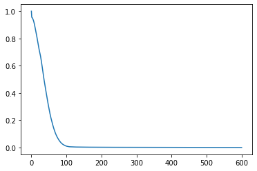
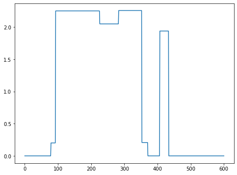
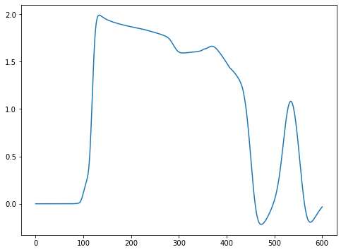
Figure 3.1: Left: Singular values of $\mathbf{A}\in\mathds{R}^{d\times d}$ modeling dissipation. Middle: Test signal $x\in\mathds{R}^{d}$. Right: Exact data $\mathbf{A}x$ for input from the middle picture. The horizontal axis in the middle and right images represents time.

Network architecture:

The architecture $(\boldsymbol{\Phi}_{\theta})_{\theta\in\theta}$ of the network resembles a one-dimensional version of the 2D Unet of [26] with one skip connection. It starts with two 1D convolutions of kernel size $7$ and $16$ channels, each followed by ReLU as the activation function. The spatial size of the feature maps is then halved using a max pooling layer. This convolution block is repeated twice, each time with twice as many filters ($32$ and $64$). By applying three convolutional upsamplings, we obtain an output of the same spatial size as the input. We concatenate the input with the output and convolve one last time so that the network is able to learn the identity for the correct signals. We keep the network architecture quite simple to reduce the computational time of the gradient computation. Dropout layers are added to prevent overfitting.

Network training:

For the training signals $x_{i}$ we take collection of the block signal similar to the ones of [8]. We construct noisy data $\mathbf{A}x_{i}+z_{i,n}$ where $z_{i,n}$ is normally distributed noise with mean zero and standard deviation $0.1$. The full training data set consists $5000$ ground truth signals $x_{i}$ and $5000$ noisy signal for each $\alpha[j,n]=j/10$ with $j\in\{1,\dots,8\}$. According to Section 2.2, the network is trained by minimizing the risk $\mathcal{L}_{n}(\theta)=\sum_{i}\sum_{j}\lVert\boldsymbol{\Phi}_{\theta}(x_{i}+r_{i,j,n})-x_{i}\rVert^{2}$. The trained network is then given by $\boldsymbol{\Phi}_{n}\coloneqq\boldsymbol{\Phi}_{\theta_{n}}$, where $\theta_{n}$ is the numerical minimizer of $\mathcal{L}_{n}$.

Numerical DD-Morozov regularization:

Reconstruction is done by numerically solving (2.1) with the noise-adaptive data-driven regularizer $\mathcal{R}_{n}\coloneqq\lVert(\operatorname{Id}-\boldsymbol{\Phi}_{n})(\cdot)\rVert^{2}/2+\lVert\mathbf{L}x\rVert_{1}$, where $\lVert\cdot\rVert_{1}$ is the $\ell^{1}$-norm and $\mathbf{L}$ is the discrete central difference operator with Neumann boundary conditions. For that purpose, we write (2.1) in the form

$$\min_{x}\|\boldsymbol{\Phi}_{n}(x)-x\|_{2}^{2}+\lambda\|\mathbf{L}x\|_{1}+\mathbf{1}_{B}(\mathbf{A}x)$$ (3.1)

with $\mathbf{1}_{B}$ denoting the indicator function of $B=\{y\in\mathds{R}^{d}\mid\|y-y_{\delta}\|\leq\delta\}$.

Optimization problem (3.1) is solved using the primal dual algorithm of [6]. With the abbreviations $F(x):=\|\boldsymbol{\Phi}_{n}(x)-x\|_{2}^{2}$, $h_{1}:=\lambda\|\cdot\|_{1}$ and $h_{2}:=\mathbf{1}_{B}$, parameters $\tau,\sigma,\rho>0$ and initial values $x^{(0)}$ and $y^{(0)}=(0,0)$ the proposed reconstruction algorithm reads

$$z^{(i+1)} :=x^{(i)}-\tau\nabla f(x^{(i)})-\tau\mathbf{L}^{*}y_{1}^{(i)}-\tau\mathbf{A}^{*}y_{2}^{(i)}$$

$$x^{(i+1)} :=\rho z^{(i+1)}+(1-\rho)x^{(i)}$$

$$w_{1}^{(i+1)} :=\operatorname{prox}_{\sigma h_{1}^{*}}(y_{1}^{(i)}+\sigma\mathbf{L}(2z^{(i+1)}-x^{(i)}))$$

$$y_{1}^{(i+1)} :=\rho w_{1}^{(i+1)}+(1-\rho)y_{1}^{(i)}$$

$$w_{2}^{(i+1)} :=\operatorname{prox}_{\sigma h_{2}^{*}}(y_{2}^{(i)}+\sigma\mathbf{A}(2z^{(i+1)}-x^{(i)}))$$

$$y_{2}^{(i+1)} :=\rho w_{2}^{(i+1)}+(1-\rho)y_{2}^{(i)}\,.$$

Here $\operatorname{prox}$ denotes the proximity mapping and $()^{*}$ the Fenchel dual. The proximity mappings $\operatorname{prox}_{\sigma h_{1}^{*}}$, $\operatorname{prox}_{\sigma h_{2}^{*}}$ can be easily computed using the relation $\operatorname{prox}_{h^{*}}+\operatorname{prox}_{h}=\operatorname{Id}$ and the known expressions for the proximity mappings of $\|\cdot\|_{1}$ and $\mathbf{1}_{B}$.

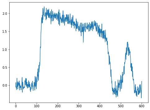
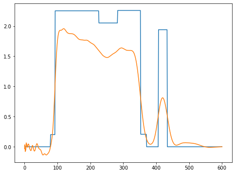
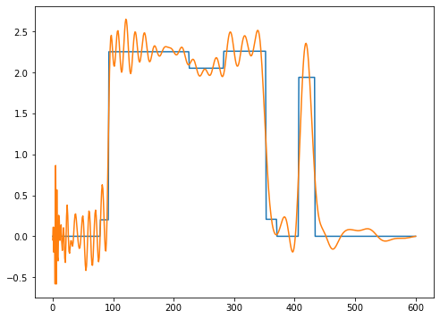
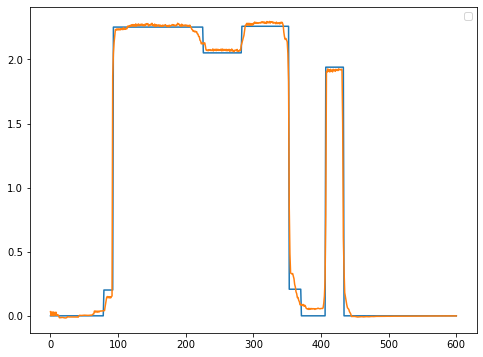
Figure 3.2: Top left: Noisy data $y_{\delta}$. Top right: BP reconstruction. Bottom left: SVD reconstruction. Bottom right: DD-Morozov reconstruction.

3.2 Results

Figure 3.2 shows results for a randomly selected block signal $x$ that is not included in the training data.The upper left image shows the noisy attenuated signal $y_{\delta}$, the upper right image shows the Backprojection (BP) reconstruction $\mathbf{A}^{T}y_{\delta}$, the lower left image shows the truncated SVD reconstruction $\mathbf{S}_{\alpha}y_{\delta}$ with $\alpha=0.1$, and the lower right image shows the results with the proposed DD-Morozov regularization.The BP reconstruction is clearly damped, while the SVD reconstruction shows strong oscillations. The corresponding reconstruction using the DD-Morozov method (1.3), (2.1) is obviously much better. Similar results have been obtained for other randomly selected training signals.

Another example is shown in Figure 3.3, where we compare the ground truth, the network prediction of the truncated SVD, the Tikhonov regularization, and the DD-Morozov regularization. As regularization parameter $\alpha$ we have chosen the optimal value for the Tikhonov method. The network prediction of the truncated SVD is the trained network $\boldsymbol{\Phi}_{n}$ applied to the SVD reconstruction. We see that the Tikhonov regularization is worse than the network prediction of the truncated SVD, and the DD-Morozov regularization best recovers information about the original signal. This suggests that the regularization property of the Morozov method, together with a properly trained network, can be superior to either of these methods.

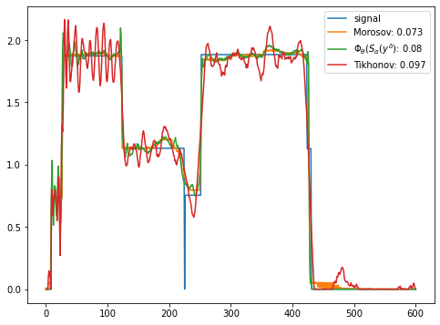
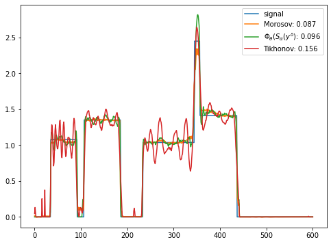
Figure 3.3: Two further randomly selected reconstruction results. In both figures, blue is the original signal, orange is the DD-Morozov reconstruction, green is the network prediction of truncated SVD, and red is the result of Tikhonov regularization.

4 Summary

In this paper, we introduced and analyzed neural network-based noise-adaptive Morozov regularization using a data-driven regularizer (NN-Morozov regularization). We performed a complete convergence analysis that also allows for noise-dependent regularizers. In addition, we established convergence in strong topology. To make our approach practical, we developed a simple yet efficient training strategy extending NETT [19]. We verified our methodology through numerical experiments, with a special focus on its application to attenuation correction for PAT. Our research can provide the basis for a broader integration of data-driven regularizers into various variational regularization techniques.

References

- [1] S. Arridge, P. Maass, O. Öktem, and C.-B. Schönlieb. Solving inverse problems using data-driven models. Acta Numerica, 28:1–174, 2019.
- [2] A. Aspri, S. Banert, O. Öktem, and O. Scherzer. A data-driven iteratively regularized Landweber iteration. Numerical Functional Analysis and Optimization, 41(10):1190–1227, 2020.
- [3] A. Aspri, Y. Korolev, and O. Scherzer. Data driven regularization by projection. Inverse Problems, 36(12):125009, 2020.
- [4] M. Benning and M. Burger. Modern regularization methods for inverse problems. Acta numerica, 27:1–111, 2018.
- [5] P. Blanchard and E. Brüning. Variational Methods in Mathematical Physics. A Unified Approach. Springer-Verlag, Berlin, 1992.
- [6] L. Condat. A primal–dual splitting method for convex optimization involving lipschitzian, proximable and linear composite terms. Journal of optimization theory and applications, 158(2):460–479, 2013.
- [7] S. Dittmer, T. Kluth, P. Maass, and D. Otero Baguer. Regularization by architecture: A deep prior approach for inverse problems. Journal of Mathematical Imaging and Vision, 62:456–470, 2020.
- [8] D. L. Donoho and I. M. Johnstone. Ideal spatial adaptation by wavelet shrinkage. Biometrika, 81:425–455, 1994.
- [9] H. W. Engl, M. Hanke, and A. Neubauer. Regularization of inverse problems, volume 375. Kluwer Academic Publishers Group, Dordrecht, 1996.
- [10] S. Göppel, J. Frikel, and M. Haltmeier. Data-proximal null-space networks for inverse problems. arXiv:2309.06573, 2023.
- [11] A. Goujon, S. Neumayer, P. Bohra, S. Ducotterd, and M. Unser. A neural-network-based convex regularizer for inverse problems. IEEE Transactions on Computational Imaging, 2023.
- [12] M. Grasmair, M. Haltmeier, and O. Scherzer. The residual method for regularizing ill-posed problems. Applied Mathematics and Computation, 218(6):2693–2710, 2011.
- [13] M. Haltmeier, R. Kowar, and L. V. Nguyen. Iterative methods for pat in attenuating acoustic media. Inverse Problems 33 (11), 2017.
- [14] M. Haltmeier and L. Nguyen. Regularization of inverse problems by neural networks. In K. Chen, C.-B. Schönlieb, X.-C. Tai, and L. Younces, editors, Handbook of Mathematical Models and Algorithms in Computer Vision and Imaging: Mathematical Imaging and Vision, pages 1–29. Springer International Publishing, Cham, 2021.
- [15] K. Ito and B. Jin. Inverse problems: Tikhonov theory and algorithms, volume 22. World Scientific, 2014.
- [16] V. K. Ivanov, V. V. Vasin, and V. P. Tanana. Theory of linear ill-posed problems and its applications, volume 36. Walter de Gruyter, 2013.
- [17] E. Kobler, A. Effland, K. Kunisch, and T. Pock. Total deep variation for linear inverse problems. In Proceedings of the IEEE/CVF Conference on computer vision and pattern recognition, pages 7549–7558, 2020.
- [18] R. Kowar and O. Scherzer. Attenuation models in photoacoustics. In Mathematical modeling in biomedical imaging II: Optical, ultrasound, and opto-acoustic tomographies, pages 85–130. Springer, 2011.
- [19] H. Li, J. Schwab, S. Antholzer, and M. Haltmeier. NETT: Solving inverse problems with deep neural networks. Inverse Problems, 36(6):065005, 2020.
- [20] S. Lunz, O. Öktem, and C.-B. Schönlieb. Adversarial regularizers in inverse problems. Advances in neural information processing systems, 31, 2018.
- [21] V. A. Morozov. Regularization Methods for Ill-Posed Problems. CRC Press, Boca Raton, 1993.
- [22] S. Mukherjee, M. Carioni, O. Öktem, and C.-B. Schönlieb. End-to-end reconstruction meets data-driven regularization for inverse problems. Advances in neural information processing systems, 34:21413–21425, 2021.
- [23] F. Natterer and F. Wübbeling. Mathematical Methods in Image Reconstruction, volume 5 of Monographs on Mathematical Modeling and Computation. SIAM, Philadelphia, PA, 2001.
- [24] D. Obmann, L. Nguyen, J. Schwab, and M. Haltmeier. Augmented NETT regularization of inverse problems. Journal of Physics Communications, 5(10):105002, 2021.
- [25] D. Riccio, M. J. Ehrhardt, and M. Benning. Regularization of inverse problems: Deep equilibrium models versus bilevel learning. arXiv:2206.13193, 2022.
- [26] O. Ronneberger, P. Fischer, and T. Brox. U-net: Convolutional networks for biomedical image segmentation. In Medical Image Computing and Computer-Assisted Intervention–MICCAI 2015: 18th International Conference, Munich, Germany, October 5-9, 2015, Proceedings, Part III 18, pages 234–241. Springer, 2015.
- [27] S. Roth and M. J. Black. Fields of experts: A framework for learning image priors. In 2005 IEEE Computer Society Conference on Computer Vision and Pattern Recognition (CVPR’05), volume 2, pages 860–867. IEEE, 2005.
- [28] O. Scherzer, M. Grasmair, H. Grossauer, M. Haltmeier, and F. Lenzen. Variational methods in imaging, volume 167 of Applied Mathematical Sciences. Springer, New York, 2009.
- [29] T. Schuster, B. Kaltenbacher, B. Hofmann, and K. S. Kazimierski. Regularization methods in Banach spaces, volume 10. Walter de Gruyter, 2012.
- [30] J. Schwab, S. Antholzer, and M. Haltmeier. Deep null space learning for inverse problems: convergence analysis and rates. Inverse Problems, 35(2):025008, 2019.
- [31] A. N. Tikhonov and V. Arsenin. Solutionsof ill-posed problems. John Wiley & Sons, Washington, D.C., 1977.