Multi-parameter Tests of General Relativity Using Bayesian Parameter Estimation with Principal Component Analysis for LISA

Abstract

In the near future, space-borne gravitational wave (GW) detector LISA can open the window of low-frequency band of GW and provide new tools to test gravity theories. In this work, we consider multi-parameter tests of GW generation and propagation where the deformation coefficients are varied simultaneously in parameter estimation and the principal component analysis (PCA) method are used to transform posterior samples into new bases for extracting the most informative components. The dominant components can be better mesured and constrained and are more sensitive to potential departures from general relativity (GR). We extend previous works by employing Bayesian parameter estimation and performing both null tests and tests with injections of subtle GR-violated signals. We also apply multi-parameter tests with PCA in the phenomenological test of GW propagation. This work complements previous works and further demonstrates the enhancement provided by the PCA method. Considering a supermassive black hole binary system as the GW source, we find that $1\sigma$ bounds of the most dominant PCA parameter can be one order of magnitude tighter than the bounds of original deformation parameter of leading frequency order. The departures less than $1\sigma$ in original parameters can yield significant departures in first 5 dominant PCA parameters.

1 Introduction

General Relativity (GR) is regarded as the most successful gravity theory due to its elegant mathematical formulation and agreement with experiments at extremely high precision [1, 2, 3, 4, 5, 6, 7, 8, 9, 10]. Whereas, difficulties of singularity and quantization problems [11, 12], as well as puzzles of dark matter and dark energy [13, 14, 15, 16] hint that GR may be not complete to describe all gravitational phenomena, which motivates people to construct alternatives theoretically and search anomalies experimentally [17, 18, 19]. In previous, extensive tests of GR have be performed from the laboratory scale [20, 3, 4], to the solar system scale [21, 2], and to the cosmological scale [5, 6, 18]. In recent years, the successful detection of gravitational waves (GWs) provide a new window to observe the universe and offer an unique tool to test gravity theories [22, 23, 24, 25, 26].

Since the first detection of GW150914 [27], more than 90 confident GW events have been captured by the LIGO, Virgo, KAGRA (LVK) Collaboration [28, 29, 30, 31]. Extensive tests of GR with GW are flourishing based on observed data from current ground detectors, such as [32, 33, 34, 35, 36]. In the near future, the space-borne GW observatories the Laser Interferometer Space Antenna (LISA), Taiji, and Tianqin are scheduled to be launched in the early 2030s [37, 38, 39]. Space-borne detectors can open the window of low-frequency GW around milli-Hertz range which encompasses abundant GW sources like supermassive black hole binaries (SMBHBs) [40], extreme mass ratio inspirals (EMRIs) [41], etc. These sources can offer invaluable information for exploring the nature of gravity [42, 43]. Forecast researches about testing GR with space-borne detectors are critical and pressing before its launch. In this work, we consider LISA as the example to discuss phenomenological parameterized tests of GW generation and propagation.

Tests of gravity theories with GW are generally approached from three perspectives, the generation, propagation, and polarization of GWs [44, 2]. In this paper, we focus on the generation and propagation of GWs. In alternative theories of gravity, the energy and angular momentum of binaries, as well as flux of them are usually different with GR [21], which can result in modifications to the binary motion and yield deformations in the waveform. For example, the dipole radiation is absent in GR but very common in plethora alternative theories [45]. In GR, GWs propagate non-dispersively with the speed of light, whereas in alternative theories this feature can be violated in various ways. Such as in Lorentz violating theories, different frequency components of GWs can propagate with different speed, which causes dispersion and distorts signals observed by detectors [46, 47, 48].

Proposals to test gravity theories in various literature may be classified into two types, performing tests and constraining model parameters in particular alternative theories [32, 49, 50] or testing in model-independent ways [51] which aims at searching any indications for deviations from predictions of GR. Since the GW waveform in particular theories is usually difficult to compute, and considering the abundance of alternative theories, theory-agnostic tests might be a more efficient way[51]. In this work, we consider two phenomenological parameterized theory-agnostic tests of GW generation and propagation which have been routinely performed on observed data by LVK [24, 23, 22]. But different with the tests implemented by LVK where phenomenological non-GR coefficients are varied separately in parameter estimation, we consider them simultaneously and employ principal component analysis (PCA) to transform posteriors of orignal modification coefficients into a set of new bases. The dominant components in the obtained PCA parameters are considered to be more sensitive to potential deviations from GR [52, 53, 54, 55, 56].

Tests with varying all deformation coefficients simultaneously are called multi-parameter tests [54]. Using the PCA method in the multi-parameter test of Post-Newtonian coefficients with GW was first introduced in the previous work [53]. A new set of coefficients can be constructed by a linear combination of original phase deformation coefficients. The new parameters can circumvent correlations among originals, and can be estimated with improved accuracy. In the paper [54], authors performed this method with selected GW events detected in first and second observing runs (O1 and O2) of LVK, and simulated non-GR signals, which shows new coefficients constructed by PCA are more sensitive to potential deviations from GR in the multi-parameter test, subtle anomalies can become significant in the posteriors of the new constructed coefficients. The works [55, 56] using Fisher method forecast performance of multi-parameter tests with PCA for future space-borne detector LISA and next generation ground-based detectors Cosmic Explorer (CE) and Einstein Telescope (ET). In this work, we extent previous work [56] by employing Bayesian parameter estimation. Furthermore, We also apply this method in the test of GW propagation.

Previous work [56] consider the multi-parameter test with PCA using Fisher matrix in which the posteriors are assumed to be Gaussian. However, as pointed out in [57], the multi-modal is one of important features of posteriors for LISA. Therefore, in order to demonstrate performance of multi-parameter tests with PCA more accurately and convincingly, we employ Bayesian inference to estimate posteriors in this work. There are various difference between space-borne detectors and ground-based detectors in parameter estimation [58]. The response function of space-borne detectors have to account for the motion of the detector and the finite dimension of arm-length. Since the duration of GW signals for space-borne detectors can be months or years, the motion of detectors can not be ignored. In the mHz band, the wavelength of GW could be comparable or less than the arm-length of detectors. Unlike the situation of ground-based detectors where a detector can be viewed as a point, one have to consider the integral of metric perturbation alone geodesic of photons for space-borne detectors. For unequal-arm interferometers, which is necessarily the case of space-borne detectors, the laser noise experience different delays for two arms, and can not be canceled out at the photon detector. The technique called time delay interferometer (TDI) has to be used to suppress laser noise.

These factors together with longer signal duration make likelihood evaluation for space-borne detectors is much more time consuming. Various methods have be adopted in previous works to alleviate the computational burden of Bayesian parameter estimation with space-borne detectors. In the work [59], the authors employed the heterodyned likelihood [60] to speed up the likelihood evaluation. By introducing a reference waveform, the likelihood can be separated as a part of slow-varying function of frequency which can be computed by a coarse interpolation, an integral of a rapidly oscillating function within fast damped envelope which can be truncated at small fraction of its full extent, and a part which can be computed ahead of Markov chain Monte Carlo (MCMC) sampling. The work [61] utilized contemporary powerful computer hardware to evaluate full likelihood in "brute-force". The authors implement the codes for waveform model and detector response function on GPU which can generate GW waveform and compute likelihood on a realistic Fourier bin width for the LISA mission in parallel and significantly reduce required computational time. In this work, we follow the method used in [57] which considers the noise-free likelihood and using interpolation to accelerate the likelihood computation. Furthermore, data from space-borne detectors are expected to be signal-dominant. Heavily overlapped signals bring new challenges to extract science information from data. Global fitting [62, 63, 64] or hierarchical fitting [65, 66] have to be used to get properties of binaries. Issues about overlapping are still under active investigation[62], therefore in this work we consider an ideal situation where the GW event has been searched out and the segment of data only contains one GW events.

In this work, we perform multi-parameter tests of GR with PCA method for LISA. We extend previous work [56] by using Bayesian parameter estimation and considering the test of GW propagation. The remainder of this paper is organized as follows. In section 2, we present a brief overview of phenomenological parameterized tests of GW generation and propagation, as well as Bayesian parameter estimation for LISA and the PCA method used to transform posteriors of deformation coefficients into a set of new bases. We consider two situations including null tests and injections of subtle deviations from GR to elaborate the advantage of the PCA method in multi-parameter tests. Results are shown and discussed in Section 3. Finally, we summarize this paper in Section 4.

2 Methodology

In this work, we consider the phenomenological parameterized tests of GW generation and propagation which have been extensively performed with current observed GW data by LVK [22, 26, 25, 24, 23]. In these tests, several phenomenological coefficients, Eq. 2 and 5, are introduced to capture any potential deviations from GR. Due to the correlations among parameters, allowing all these coefficients to vary simultaneously in the parameter estimation will yield less informative posterior. In the tests performed by LVK, only one coefficient is allowed to vary at a time.

Previous works [53] pointed out that such correlations can be reduced by transforming the deformation coefficients into a set of new orthogonal bases obtained from PCA, which allow people to perform multi-parameter tests, i.e. estimating all deformation coefficients simultaneously. The effectiveness of multi-parameter tests with PCA has been shown in [54, 67] in which tests of GW generation using GW data detected by current ground based detectors are demonstrated. Using the Fisher method, previous works [68, 55, 56, 52] present the forecasts of multi-parameter tests considering future space based detectors, next generation ground based detectors, and multi-band observations through synergies of both.

In this paper, we extend previous works by using Bayesian parameter estimation to further illustrate that the PCA have more sensitivity to potential deviations in multi-parameters tests, and including the phenomenological parameterized test of GW propagation.

2.1 Multi-parameter tests of GW generation and propagation

In the early inspiral period where orbital velocities of binaries are sufficiently low, motion of compact binaries can be well described by post-Newtonian (PN) formalism in which GW waveform is given by the form of expansion in terms of $v=(\pi Mf)^{1/3}$ where $M$ is the total mass of the binary[69]. Since potential deviations in GW phase can be accumulated as orbital evolution, GW observations are more sensitive to phase than amplitude in general. Tests of GW generation usually focus on GW phase. The 3.5 PN phase of GW waveform [70] has the form of

$$\Phi_{\mathrm{PN}}(f)=2\pi ft_{\mathrm{c}}-\varphi_{\mathrm{c}}-\frac{\pi}{4}+\frac{3}{128\eta}v^{-5}\sum_{i=0}^{7}\left[\varphi_{i}+\varphi_{il}\log v\right]v^{i}$$ (1)

where $t_{\mathrm{c}}$ and $\varphi_{\mathrm{c}}$ are the time and phase at coalescence, $\eta$ is the symmetric mass ratio, coefficients $\varphi_{i}$ and $\varphi_{il}$ are constants determined by intrinsic parameters of binaries.

In order to capture potential deviation from GR, deformation coefficients

$$\{\delta\varphi_{0},\delta\varphi_{2},\delta\varphi_{3},\delta\varphi_{4},\delta\varphi_{5l},\delta\varphi_{6},\delta\varphi_{6l},\delta\varphi_{7}\}$$ (2)

are introduced through

$$\varphi_{i}\rightarrow\varphi_{i}^{\mathrm{GR}}(1+\delta\varphi_{i}),\;\text{or}\ \varphi_{il}\rightarrow\varphi_{il}^{\mathrm{GR}}(1+\delta\hat{\varphi}_{il}).$$ (3)

The deformation coefficient of 2.5 PN non-logarithmic term is not included due to its degeneration with coalescence phase. Besides, following [56] we have also not considered the 0.5 PN deformation coefficient $\delta\varphi_{1}$. These deformation coefficients are treated as free parameters when performing parameter estimation. Potential departures from GR can be reflected by posteriors deviating from zero. In this work, intermediate and merger-ringdown deformation coffecients $\alpha_{i}$ and $\beta_{i}$ are not considered.

The model-agnostic phenomenological parameterized test of GW propagation utilizes a phenomenological modified GW dispersion relation [47] which takes the form of

$$E^{2}=p^{2}+A_{\alpha}p^{\alpha},$$ (4)

where $E$ and $p$ are the energy and momentum of GWs, $A_{\alpha}$ are phenomenological coefficients. In this work, we follow tests performed by LVK [24, 23, 22] and consider cases of $\alpha$ running form 0 to 4 with cadence of 0.5 excluding the case of $\alpha=2$ where the speed of GW is independent with frequency. Thus the dephasing is a constant and completely degenerate with the arriving time of GW transients, and can only be constrained with the present of electromagnetic counterparts.

The adding power-law terms $A_{\alpha}p^{\alpha}$ in Eq. 4 make different frequency components of GWs propagate with different speed, and distort the observed GW waveforms. Assuming the waveform in local wave zone is well-described by GR, only considering the dispersion effect during the propagation, the deformation in phase have been given as [47]

$$\delta\Phi_{\alpha}(f)=\mathrm{sign}(A_{\alpha})\begin{cases}\frac{\pi(1+z)^{\alpha-1}D_{\alpha}}{(\alpha-1)}\lambda_{\alpha}^{\alpha-2}f^{\alpha-1},\quad&\alpha\neq 1\\ \frac{\pi D_{\alpha}}{\lambda_{A}}\ln(\pi\mathcal{M}f),&\alpha=1\end{cases},$$ (5)

where $\lambda_{A}\equiv h|A_{\alpha}|^{1/(\alpha-2)}$, and $D_{\alpha}$ is defined as

$$D_{\alpha}=\frac{(1+z)^{1-\alpha}}{H_{0}}\int\frac{(1+z^{\prime})^{\alpha-2}dz^{\prime}}{\sqrt{\Omega_{\mathrm{M}}(1+z^{\prime})^{3}+\Omega_{\Lambda}}}.$$ (6)

In the computation, we use $H_{0}=67.66\mathrm{km}/(\mathrm{Mpc}\cdot\mathrm{s})$, $\Omega_{\mathrm{M}}=0.3111$, and $\Omega_{\Lambda}=0.6889$ for the values of Hubble constant, matter and dark energy density parameters, which are taken from Planck 2018 results [71]. For the convenience to perform the multi-parameter test with PCA, we consider a parameterization slightly different with LVK. The phase deformation Eq. 5 can be rewritten as

$$\delta\Phi_{\alpha}(f)=\begin{cases}\delta\phi_{\alpha}\frac{(1+z)^{\alpha-1}}{(\alpha-1)\pi^{\alpha-2}}\left(\frac{10^{7}M_{\odot}}{M}\right)^{\alpha-1}\left(\frac{D_{\alpha}}{1\mathrm{Gpc}}\right)v^{3(\alpha-1)},\quad&\alpha\neq 1\\ \delta\phi_{\alpha}\frac{D_{\alpha}}{1\mathrm{Gpc}}\pi\ln(\pi\mathcal{M}f),&\alpha=1\end{cases}.$$ (7)

where

$$\delta\phi_{\alpha}=\frac{1{\rm Gpc}(10^{7}M_{\odot})^{1-\alpha}}{\lambda_{A}^{2-\alpha}}$$ (8)

is the parameters varied in parameter estimation.

We employ the waveform model IMRPhenomD [72, 70] as the basis. The deformations of generation Eq. 3 are added into the PN expansion structure, and the deformation of propagation Eq. 7 are added to the overall waveform.

2.2 Bayesian parameter estimation

Bayesian parameter estimation is based on Bayes theorem

$$p(\boldsymbol{\theta}|\boldsymbol{d},M)=\frac{\pi(\boldsymbol{\theta}|M)p(\boldsymbol{d}|\boldsymbol{\theta},M)}{p(\boldsymbol{d}|M)},$$ (9)

where $\boldsymbol{d}$ denotes observed data, $M$ and $\boldsymbol{\theta}$ represents the underlying model and parameters required to describe the model. $p(\boldsymbol{\theta}|\boldsymbol{d},M)$ is the posterior which describes the probability distribution of the model parameters based on the observed data, and is the goal of parameter estimation. The posterior is a combination of two elements: the prior $p(\boldsymbol{\theta}|M)$ which implies our prior knowledge about the model parameters ahead of observation, and the likelihood $p(\boldsymbol{d}|\boldsymbol{\theta},M)$ which represents the probability of a realization of time series observed by detectors given a particular set of model parameter values. The evidence $p(\boldsymbol{d}|M)$ is a constant normalizing factor and can also be used in model comparison.

If the noise is stationary, Gaussian and uncorrelated, the likelihood can be written as [73]

$$p(\boldsymbol{d}|\boldsymbol{\theta},M)\propto\exp\left[-\frac{1}{2}\sum_{i}\left\langle\boldsymbol{h}(\boldsymbol{\theta})-\boldsymbol{d}|\boldsymbol{h}(\boldsymbol{\theta})-\boldsymbol{d}\right\rangle\right],$$ (10)

where $\boldsymbol{h}(\boldsymbol{\theta})$ is the detector responses for a waveform with a set of parameter values $\boldsymbol{\theta}$, $\boldsymbol{d}$ is the observed data, $i$ represent dependent measurements, here is different TDI channels which will be discussed in more detail below. The angle brackets denote the noise-weighted inner product defined as

$$\left\langle\boldsymbol{a}|\boldsymbol{b}\right\rangle=4\mathfrak{R}\int\frac{a(f)b^{*}(f)}{S_{n}(f)}\ {\rm d}f,$$ (11)

with the noise power spectral density (PSD) $S_{n}(f)$. In this paper, we consider the noise model SciRDv1 described in [74].

The response of space-borne detectors to GWs have many difference in various aspects comparing with ground-based detectors. For ground-based detectors, the wavelength of $\sim 500\mathrm{Hz}$ GWs is much longer than arm-length of detectors. The size of detectors can be neglected. For space-borne detectors, like LISA, the designed arm-length $2.5\times 10^{6}\mathrm{km}$ corresponds to a frequency $f_{*}=0.12\mathrm{Hz}$ which is usually called the transfer frequency. If the frequency of GW is above the transfer function, in the journey of a laser photon from emission to reception, there may be multiple wavelengths of GW passing through the detector, which can result in the optical length variation canceled out by GW itself. To derive the response of a signal laser link, we need to perform integral of the metric perturbation along the geodesic of a photon [75, 76, 77]. The response of a single link in frequency domain is given by

$$\tilde{y}_{slr}(f)=i\pi fL\ \mathrm{sinc}\left[\pi fL(1-\mathbf{k}\cdot\mathbf{n}_{l})\right]\exp\left\{-i\pi f[L+\mathbf{k}\cdot(\mathbf{p}_{r}+\mathbf{p}_{s})]\right\}\mathbf{n}_{l}\cdot\mathbf{h}^{\rm TT}(f)\cdot\mathbf{n}_{l}.$$ (12)

We follow the notation used in [57] where $l$ denote the link sent from node $s$ and received by node $r$, $\mathbf{p}_{r}$ and $\mathbf{p}_{s}$ are positions of the two nodes, unit vectors $\mathbf{k}$ and $\mathbf{n}_{l}$ point to the direction of the GW source and the direction of the laser link respectively. It is an important difference of space-borne detectors comparing with ground-based detectors that the signal duration is longer during which the motion of detectors can not be neglected. The vectors of detector constellation $\mathbf{n}_{l}$, $\mathbf{p}_{s}$ and $\mathbf{p}_{r}$ in Eq. 12 are time-dependent. For the signals like SMBHBs which will merge in the LISA sensitive band, the orbital evolution of GW source is much faster than the orbital evolution the detectors, the generalized stationary phase approximation can be used to obtain the single link response in frequency domain [58], which directly substitutes the time in Eq. 12 by the time-frequency correspondence

$$t_{f}=-\frac{1}{2\pi}\frac{\mathrm{d}\Phi(f)}{\mathrm{d}f},$$ (13)

where $\Phi$ is the phase of GW. There is another difference that space-borne detectors are unequal-arm interferometers. The laser noise which is stronger than GW signals a few orders will experience different delays in the two arms, thus can not be canceled by itself at the photo detector backend. TDI has to be used to construct observables by time-shifting and combining single link responses (Eq. 12) [78]. The 1.5 generation TDI observable $X$ in frequency domain takes the form of [57]

$$X=[y_{321}+zy_{123}-(y_{231}+zy_{132})](1-z^{2}),$$ (14)

where $z=\exp[i2\pi fL]$. The other two observables $Y$, $Z$ can be obtained by cyclic permutation of indices. The uncorrelated channels are given by combinations

$$A =\frac{1}{\sqrt{2}}(Z-X),$$ (15)

$$E =\frac{1}{\sqrt{6}}(X-2Y+Z),$$

$$T =\frac{1}{\sqrt{3}}(X+Y+Z).$$

Although it is the unequal arm-length that that make it necessary to employ the TDI technique, in terms of noise feature of TDI observables, it is still proper to assume that the arm-length of each link is equal and constant [79]. And with additional assumption that the noise of the same type have the same PSD, the noise of $A$, $E$, $T$ can be described by [79]

$$S_{A,E} =8\sin^{2}(2\pi fL){[2+\cos(2\pi fL)]S_{\rm OMS}+[6+\cos(4\pi fL)+4\cos(2\pi fL)]S_{\rm acc}},$$ (16)

$$S_{T} =32\sin^{2}(2\pi fL)\sin^{2}(\pi fL)[S_{\rm OMS}+4\cos(\pi fL)S_{\rm acc}],$$

where $S_{\rm OMS}$ and $S_{\rm acc}$ denote the noise of optical metrology system and acceleration noise. We consider the noise model SciRDv1 given in [74] which reads

$$\sqrt{S_{\rm OMS}}(f) =15\times 10^{-12}\frac{2\pi f}{c}\sqrt{1+\left(\frac{2\times 10^{-3}}{f}\right)^{4}}\left[\frac{1}{\sqrt{\mathrm{Hz}}}\right],$$ (17)

$$\sqrt{S_{\rm acc}}(f) =\frac{3\times 10^{-15}}{2\pi fc}\sqrt{1+\left(\frac{0.4\times 10^{-3}}{f}\right)^{2}}\sqrt{1+\left(\frac{f}{8\times 10^{-3}}\right)^{4}}\left[\frac{1}{\sqrt{\mathrm{Hz}}}\right].$$

.

In practice, we use lisabeta [57] to compute detector responses and evaluate likelihood. We add the modification of Eq. 3 and Eq. 7 into the GW phase and time-frequency relation based on the waveform model IMRPhenomD [72, 70]. To estimate the posterior, we employ the nested sampler dynesty [80] with MCMC evolution implemented in bilby [81]. As mentioned in above, the response of space-borne detectors to GWs is more complex, and the longer signal duration leads to more frequency points required to be computed when evaluating the likelihood. The full Bayesian parameter estimation is extremely computational expensive for space-borne detectors. lisabeta [57] circumvent this problem by considering a noise-free likelihood and using interpolation on a sparse frequency grid. While the likelihood without noise realization can not be used in analyses of real data, it can still capture the correlation between the parameters and multi-modality of posteriors.

2.3 Principal component analysis

Using Bayesian framework and stochastic sampling algorithm discussed in last subsection, we can obtain posterior samples whose densities can approximate to the posterior probability distributions of binary properties and deformation coefficients introduced in Section 2.1. However, varying all deformation coefficients simultaneously in parameter estimation can yields less informative posteriors due to correlation among them. the PCA method can remedy this problem by transform deformation coefficients into new bases which are constructed by a linear combination of original deformation coefficients [52, 53, 54, 55, 56]. The new constructed parameters can be measured and constrained better by observed data, thus are more sensitive to potential deviation from GR. The procedure for PCA is briefly reviewed in following.

The covariance matrix for posterior samples of deformation coefficients obtained by Bayesian parameter estimation with marginalizing over GR parameters of binaries can be given by

$$C_{jk}=\left\langle\left(\delta\varphi_{j}-\langle\delta\varphi_{j}\rangle\right)\left(\delta\varphi_{k}-\langle\delta\varphi_{k}\rangle\right)\right\rangle.$$ (18)

Here we use the deformation coefficients $\delta\varphi_{i}$ in GW generation test (Eq. 2) for example, the procedure is same for $\delta\phi_{\alpha}$ in the test of GW propagation. $\delta\varphi_{j}$ and $\delta\varphi_{k}$ denote posterior samples of different deformation coefficients and the angle brackets represent the expectation value of the random variable. Diagonalizing the covariance matrix $C_{ij}$ of deformation coefficients, we can express this matrix by its eigenvalues and eigenvectors

$$\mathbf{C}=\mathbf{U}\mathbf{S}\mathbf{U}^{T},$$ (19)

where $\mathbf{S}$ is a diagonal matrix with eigenvalues of $\mathbf{C}$ as its diagonal elements, $\mathbf{U}$ has eigenvectors of $\mathbf{C}$ as its columns. The eigenvectors of $\mathbf{C}$ represent a new set of bases of deformation parameters, and original deformation parameters can be transformed into the new bases by

$$\delta\varphi^{\rm PCA}_{i\text{-th}}=\sum_{k}\alpha_{ik}\delta\varphi_{k},$$ (20)

where $\alpha_{ik}$ are columns of $\mathbf{U}$, namely eigenvectors of covariance matrix $\mathbf{C}$, and $\delta\varphi_{k}$ are the original deformation coefficients. The eigenvectors of $\mathbf{C}$ define a set of new bases of deformation parameters. These new bases are different components of the posterior samples with different amounts of information, where the magnitude of each corresponding eigenvalue implies how principal the component is. Samples of dominant components carry the most information of posteriors, thus have smaller variance and can be measured and constrained better. As we will see in next section, the dominant PCA parameters can be more sensitive to potential violations of GR.

3 Results and discussions

Following [56], we consider a SMBHB system with total mass of $7\times 10^{5}M_{\odot}$ and mass ratio of 2. The aligned dimensionless spins of two components are $0.3$ and $0.2$ respectively. As mention in Section 2.2, we add non-GR modification based on the waveform model IMRPhenomD in which the in-plane spins are not considered. We consider two situations including null tests and tests with injections of subtle deviations from GR. The detailed results are presented in following.

3.1 The null tests

We first perform the null test of GW generation. The GR signal is injected, while the waveform with deformation coefficients of Eq. 2 is used to recover properties of the binary. The 11 GR parameters and 8 deformation parameters are varied in parameter estimation. The posteriors of all deformation coefficients after marginalizing over other GR parameters are shown in Fig. 1. Using the PCA method, the posterior samples can be transformed into a set of new bases. Results after this transformation are shown in Fig. 2. For convenience of quantitative comparison, the standard deviations of posterior samples are summarized in Tab. 1.

As dicsussed in Sec. 2.3, the PCA method transform original posterior samples into new bases. The amount of information carried by posteriors of each new bases is denoted by the magnitude of corresponding eigenvalues of the covariance matrix $\mathbf{C}$ of posterior samples. The new bases of parameter space can be viewed as the components of posterior samples. How informative the components are corresponds the size of error bars. The more dominant components can be measured and constrained better, and are more sensitive to penitential violations of GR. As can be seen by comparing Fig. 1 and 2, the variance of the posterior of dominant PCA parameters shrinks significantly, even comparing the posterior of the most leading order PN deformation parameter. Quantitatively, the most dominant PCA parameter can be constrained to $\sim\mathcal{O}(10^{-4})$ which is tighter an order of magnitude than the constraints of the leading PN deformation parameter. This result is in the agreement with the previous expectations for multi-parameters tests of GW generation using Fisher matrix [56] which reports the two most dominant PCA parameters can be bounded to $\sim\mathcal{O}(10^{-4})$.

Next, we focus on the null test of GW propagation. The difference between the test of generation is that the deformation Eq. 7 is added to the overall waveform rather the only PN expansion structure of inspiral. The operation on posterior samples as discussed in Sec. 2.3 is the same with the test of generation. The posteriors of original deformation parameters and the PCA parameters are shown in Fig. 3 and 4. The standard deviations are collected in Tab. 2 for quantitative comparison. Comparing with results of the test of generation, there is a difference that the constrains on original dispersion parameters are not monotonic with orders of frequency. This is due to the parameterization of Eq. 7 we considered. Additional factors involving the $(\alpha-1)$ power term of source mass will change with the orders of frequency. Observing the results of PCA parameters, the conclusion is the same with the test of generation. The dominant PCA parameters can be constrained better than original dispersion parameters in multi-parameters tests. If there are penitential violations of GR, PCA parameters will be more sensitive to the departures.

From null tests, we can find that the new parameters constructed by PCA method can be constrained better. Thus the PCA parameters are expected to be more sensitive to possible deviations from GR. In order to elaborate the virtue of the PCA method more explicitly, we then consider the situation with injections of mild deviations from GR.

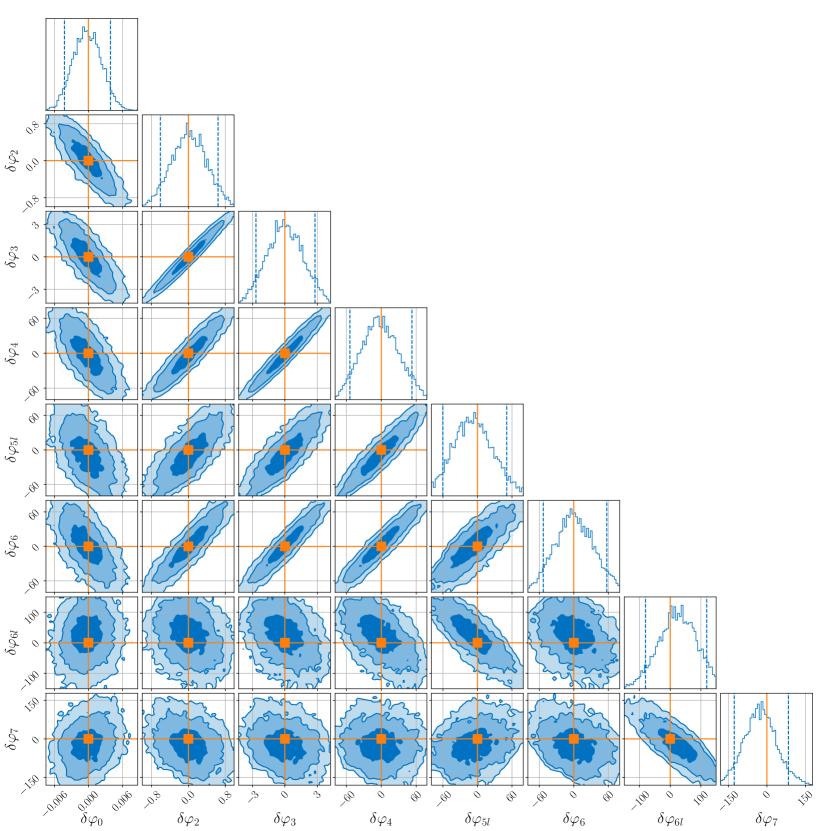
Figure 1: Posteriors of 8 PN deformation parameters after marginalizing over other GR parameters in the null test of GW generation. The orange solid lines denote the injected GR values, and the dashed vertical lines denote $5\%$ and $95\%$ quantiles.

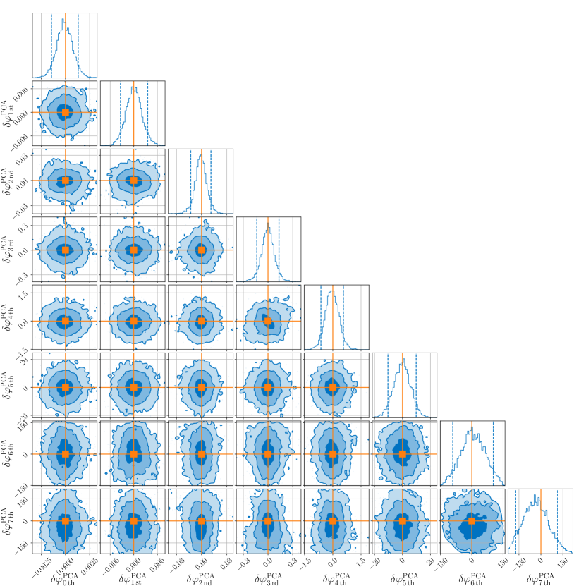
Figure 2: Probability distributions of PCA parameters which are obtained by transforming posterior samples of original PN deformation parameters shown in Fig. 1 into a set of new bases constructed by the PCA method. Comparing with Fig. 1, it can be found the first few dominant PCA parameters can be better constrained and could be more sensitive to potential deviations from GR. The explicit values of $1\sigma$ bounds can be found in Tab. 1.

PN deformation parameters		PCA parameters
$\delta\varphi_{0}$	0.00246	$\delta\varphi^{\rm PCA}_{0\,\rm th}$	0.000841
$\delta\varphi_{2}$	0.372	$\delta\varphi^{\rm PCA}_{1\,\rm st}$	0.00207
$\delta\varphi_{3}$	1.62	$\delta\varphi^{\rm PCA}_{2\,\rm nd}$	0.00747
$\delta\varphi_{4}$	31.5	$\delta\varphi^{\rm PCA}_{3\,\rm rd}$	0.0834
$\delta\varphi_{5l}$	33.2	$\delta\varphi^{\rm PCA}_{4\,\rm th}$	0.369
$\delta\varphi_{6}$	32.7	$\delta\varphi^{\rm PCA}_{5\,\rm th}$	6.14
$\delta\varphi_{6l}$	59.8	$\delta\varphi^{\rm PCA}_{6\,\rm th}$	57.9
$\delta\varphi_{7}$	62.5	$\delta\varphi^{\rm PCA}_{7\,\rm th}$	85.1

Table 1: Standard deviation $\sigma$ for posterior samples of PN deformation parameters and constructed PCA parameters in the null test of GW generation. It can be seen that the first few dominant PCA parameters are measured and constrained better, which implies they can be more sensitive to potential departures of GR.

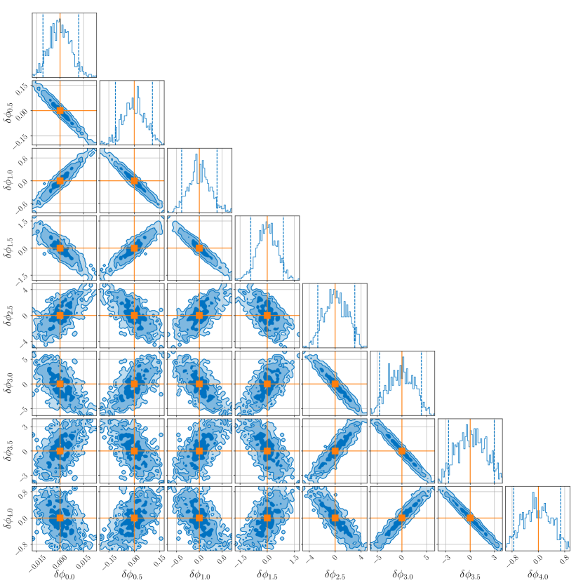
Figure 3: Posteriors of dispersion deformation parameters in the null test of GW propagation. Same with previous cases, the orange solid lines and blue dashed lines denote injected GR values and quantiles of $5\%,95\%$ repectively.

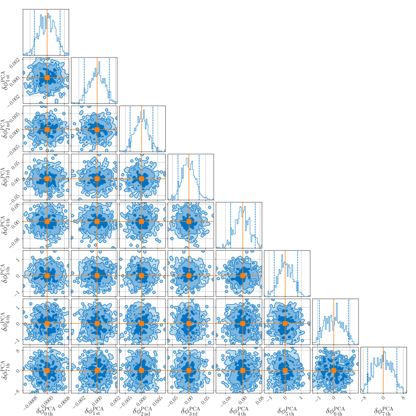
Figure 4: Distributions of posterior samples after PCA in the null test of propagation. Through the procedure discussed in Sec. 2.3, posterior samples of dispersion parameter can be transformed into a set of new bases where the information contained in posteriors is redistributed in different components. The first few dominant components include most information, thus have smaller deviations. These dominant components can be measured better by data, and are more sensitive to potential violations of GR.

dispersion parameters		PCA parameters
$\delta\phi_{0.0}$	0.00687	$\delta\phi^{\rm PCA}_{0\,\rm th}$	0.000370
$\delta\phi_{0.5}$	0.0661	$\delta\phi^{\rm PCA}_{1\,\rm st}$	0.000828
$\delta\phi_{1.0}$	0.284	$\delta\phi^{\rm PCA}_{2\,\rm nd}$	0.00210
$\delta\phi_{1.5}$	0.546	$\delta\phi^{\rm PCA}_{3\,\rm rd}$	0.0203
$\delta\phi_{2.5}$	1.76	$\delta\phi^{\rm PCA}_{4\,\rm th}$	0.0348
$\delta\phi_{3.0}$	2.59	$\delta\phi^{\rm PCA}_{5\,\rm th}$	0.440
$\delta\phi_{3.5}$	1.71	$\delta\phi^{\rm PCA}_{6\,\rm th}$	0.563
$\delta\phi_{4.0}$	0.429	$\delta\phi^{\rm PCA}_{7\,\rm th}$	3.58

Table 2: Similar to Tab. 1, standard deviation for posterior samples of GW dispersion parameters and their PCA parameters are shown here. Due to the parameterization of Eq. 7 considered here, where additional factors involving the $(\alpha-1)$ power term of source mass will change with the orders of frequency, the constrains on original dispersion parameters are not monotonic with orders of frequency like PN deformaiton parameters. But we can obtain the same conclusion that PCA parameters can be constrained better and are more capable to capture potential GR violation.

3.2 Detecting possible deviations from GR

In the last subsection, it has been shown that dominant PCA parameters can be measured and constrained better, thus can be more sensitive to potential GR violations. In this subsection, we verify this conclusion by considering injections of subtle deviations from GR which may be difficult to detected by original deformation parameters. But by using the PCA method, the degeneracy among deformation parameters can be broken in new constructed PCA parameters, thus the subtle departures in original parameters can leave significant indications in first few dominant PCA parameters.

The methods for recovering source parameters and manipulating posterior samples are the same with null tests. The difference is that injections of subtle GR violations are considered in this subsection. As shown in Fig. 5, the violin-plots with blue face represent posteriors of original PN deformation parameters where the gray dashed lines denote the injection values and red for GR values, the error bars are determined by $5\%$ and $95\%$ quantiles. The PCA parameters are shown by orange face. It can be clearly seen that the subtle GR violations which are difficult to be identified by original PN deformation parameters can lead significant departures in the first 5 dominant PCA parameters. For convenience of quantitative comparison, the distance between GR values and posterior medians in the unit of the standard deviation of posterior samples are shown in Tab. 3. The violations less than $1\sigma$ in original PN deformation parameters can lead significant departures in the first 5 dominant PCA parameters. Similarly, the results for the test of propagation are presented in Fig. 6 and Tab. 4. As expected, though the injections only have very slight GR violation, the first 5 dominant PCA parameters can significantly deviate from GR values, which demonstrates that the PCA parameters are more capable to capture potential GR violations.

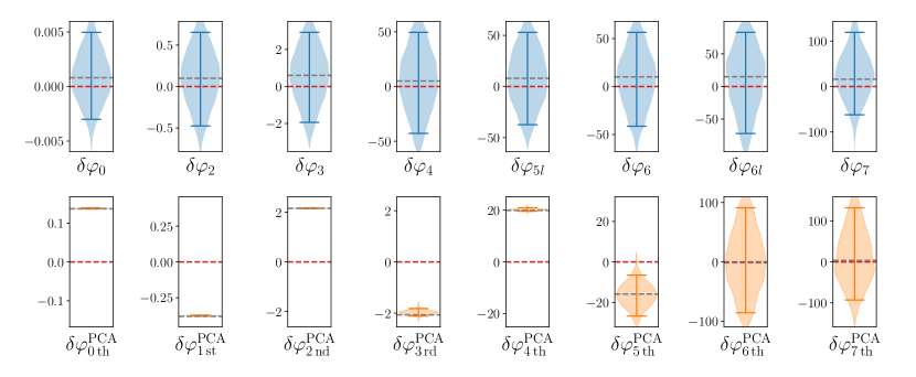
Figure 5: Violin plots for posteriors of PN deformation parameters in the test with injection of subtle GR violation. The red lines denote GR values and the gray lines denote injection values. The errors bars are determined by $5\%$ and $95\%$ quantiles of posterior samples. The original PN deformation parameters are shown by blue, while the PCA parameters are presented by orange. It can be clearly seen that small departures from GR can be identified by the PCA method in high significance.

PN deformation parameters		PCA parameters
$\delta\varphi_{0}$	$0.348\sigma$	$\delta\varphi^{\rm PCA}_{0\,\rm th}$	$151\sigma$
$\delta\varphi_{2}$	$0.307\sigma$	$\delta\varphi^{\rm PCA}_{1\,\rm st}$	$-172\sigma$
$\delta\varphi_{3}$	$0.395\sigma$	$\delta\varphi^{\rm PCA}_{2\,\rm nd}$	$205\sigma$
$\delta\varphi_{4}$	$0.156\sigma$	$\delta\varphi^{\rm PCA}_{3\,\rm rd}$	$-21.3\sigma$
$\delta\varphi_{5l}$	$0.316\sigma$	$\delta\varphi^{\rm PCA}_{4\,\rm th}$	$48.7\sigma$
$\delta\varphi_{6}$	$0.286\sigma$	$\delta\varphi^{\rm PCA}_{5\,\rm th}$	$-2.68\sigma$
$\delta\varphi_{6l}$	$0.291\sigma$	$\delta\varphi^{\rm PCA}_{6\,\rm th}$	$0.0232\sigma$
$\delta\varphi_{7}$	$0.445\sigma$	$\delta\varphi^{\rm PCA}_{7\,\rm th}$	$0.132\sigma$

Table 3: The distance between GR values and posterior medians in the unit of standard deviation for the GW generation test with subtle GR violations are presented above, which can show the improvement of the capability to detect potential GR violations through the PCA method. Since the degeneracy is broken in constructed PCA parameters, the subtle deviations in original PN deformation parameters can leave significant indication of departures in PCA parameters.

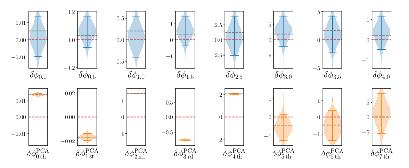
Figure 6: Similar to Fig. 5, violin plots of the test for GW propagation with injections of subtle violations of GR. Small deviations in original dispersion parameters can yeild significant departures in first 5 dominant PCA parameters.

dispersion parameters		PCA parameters
$\delta\phi_{0.0}$	$0.246\sigma$	$\delta\phi^{\rm PCA}_{0\,\rm th}$	$28.2\sigma$
$\delta\phi_{0.5}$	$0.903\sigma$	$\delta\phi^{\rm PCA}_{1\,\rm st}$	$-8.65\sigma$
$\delta\phi_{1.0}$	$0.217\sigma$	$\delta\phi^{\rm PCA}_{2\,\rm nd}$	$161\sigma$
$\delta\phi_{1.5}$	$0.970\sigma$	$\delta\phi^{\rm PCA}_{3\,\rm rd}$	$-35.9\sigma$
$\delta\phi_{2.5}$	$0.258\sigma$	$\delta\phi^{\rm PCA}_{4\,\rm th}$	$55.4\sigma$
$\delta\phi_{3.0}$	$0.962\sigma$	$\delta\phi^{\rm PCA}_{5\,\rm th}$	$-1.28\sigma$
$\delta\phi_{3.5}$	$0.473\sigma$	$\delta\phi^{\rm PCA}_{6\,\rm th}$	$-0.920\sigma$
$\delta\phi_{4.0}$	$0.708\sigma$	$\delta\phi^{\rm PCA}_{7\,\rm th}$	$0.361\sigma$

Table 4: Similar to Tab. 3, the distance between GR values and posterior medians in the test of GW propagation are collected in this table for quantitative comparison.

4 Summary

GW observations provide new tools to explore the nature of universe. Current ground-based GW detectors have obtained fruitful accomplishments and been leading to a paradigm shift in researches of astrophysics, cosmology and gravity. Space-borne detectors will open the window of low-frequency GW in the near future. Testing gravitational theories is one of the most important scientific goals of space-borne detectors. Previous works [52, 53, 54, 55, 56] have pointed out that using the PCA method can improve the capability of detecting potential violations of GR in multi-parameters tests. In this work, we complement previous work [56] by using Bayesian parameter estimation and extend this method to the test of GW propagation.

The phenomenological parameterized tests [47, 82] of GW generation and propagation have been routinely performed by LVK with current detected GW events. Due to correlations among deformation coefficients, varying all coefficients simultaneously can lead to less informative posteriors. Therefore, in the implementation of LVK [24, 23, 22], only one deformation coefficient is allowed to vary at a time in parameter estimation. However, it is proposed in [53] that the PCA method can remedy this problem. A new set of bases are constructed in the PCA method, among which the information carried by posterior samples are redistributed. The dominant PCA parameters contain the most information of posteriors, thus have smaller variance, which means these parameters can be measured and constrained better, and be more sensitive to potential GR violations. The PCA method allow people to perform multi-parameter tests, i.e. varying all deformation parameters simultaneously, while still getting informative constrains on departures from GR through the dominant PCA parameters.

In this work, we consider multi-parameter tests with space-borne detector LISA, extend previous work [56] by using Bayesian parameter estimation and apply the similar method to the test of GW propagation. Following the previous work [56], we also consider a SMBHB system as GW source, and employ lisabeta to evaluate the likelihood which incorporates the motion of detector, the TDI combination, and the finite-size of arm-length. Nested sampler dynesty with sampling method implemented in bilby is used to estimate the posteriors of source properties. For the waveform model, we consider the phenomenological parameterized tests of GR generation and propagation based on IMRPhenomD. After the sampling process, the posterior samples of deformation coefficients are transformed to new bases given by the PCA method. The dominant new PCA parameters can be constrained better, thus can be more sensitive potential GR violation. We perform both null tests where GR signals are injected and tests with subtle departures from GR. From the obtained results, in null tests we can find that the $1\sigma$ bounds of the most dominant PCA parameters can be an order of magnitude tighter than the original parameter of leading order of frequency. In the tests with subtle departures, the violations less than $1\sigma$ can yield significant departures in first 5 dominant PCA parameters.

It is worth noting that the phenomenological parameterized tests capture any violations of the waveform model used in parameter estimation. Not only anomalies beyond GR but also systematic errors of the waveform and unmodeled effects like eccentricity [83] or environmental effects [84], etc. It is required further investigations to explore the influence of systematic errors and unmodeled effects on multi-parameter tests of GR. Additionally, although the noise-free likelihood [57] considered in this work can capture the features of multi-modality and correlations among parameters, it can not be used to analysis real GW data. In future works, likelihood with noise realization and more realistic data analysis problems like signal overlapping, data gap, unstationary noise, etc. need to be considered.

5 Acknowledgements

R.N. is supported in part by the National Key Research and Development Program of China Grant No.2022YFC2807303. W.Z. is supported by the National Key Research and Development Program of China Grant No.2021YFC2203102 and 2022YFC2200100, NSFC Grants No. 12273035 and 11903030, the Fundamental Research Funds for the Central Universities. C.F. is supported by the National Key Research and Development Program of China Grant No. 2022YFC2204603 and by the starting grant of USTC. The numerical calculations in this paper have been done on the supercomputing system in the Supercomputing Center of University of Science and Technology of China. Data analyses and results visualization in this work made use of lisabeta [57], Bilby [81], Dynesty [80], LALSuite [85], PESummary [86], NumPy [87, 88], and matplotlib [89].

References

- [1] E. Berti, E. Barausse, V. Cardoso, L. Gualtieri, P. Pani, U. Sperhake et al., Testing general relativity with present and future astrophysical observations, Class. Quantum Grav. 32, 243001 (2015) (2015) [1501.07274].
- [2] C.M. Will, The confrontation between general relativity and experiment, Living Reviews in Relativity 17 (2014) .
- [3] C.D. Hoyle, U. Schmidt, B.R. Heckel, E.G. Adelberger, J.H. Gundlach, D.J. Kapner et al., Submillimeter test of the gravitational inverse-square law: A search for “large” extra dimensions, Physical Review Letters 86 (2001) 1418.
- [4] E.G. Adelberger, New tests of einstein's equivalence principle and newton's inverse-square law, Classical and Quantum Gravity 18 (2001) 2397.
- [5] B. Jain and J. Khoury, Cosmological tests of gravity, Annals of Physics 325 (2010) 1479.
- [6] K. Koyama, Cosmological tests of modified gravity, Reports on Progress in Physics 79 (2016) 046902.
- [7] I.H. Stairs, Testing general relativity with pulsar timing, Living Reviews in Relativity 6 (2003) .
- [8] R.N. Manchester, Pulsars and gravity, International Journal of Modern Physics D 24 (2015) 1530018.
- [9] N. Wex, Testing relativistic gravity with radio pulsars, 1402.5594.
- [10] M. Kramer, Pulsars as probes of gravity and fundamental physics, in The Fourteenth Marcel Grossmann Meeting, WORLD SCIENTIFIC, nov, 2017, DOI.
- [11] B.S. DeWitt, Quantum theory of gravity. i. the canonical theory, Physical Review 160 (1967) 1113.
- [12] C. Kiefer, Why quantum gravity?, in Approaches to Fundamental Physics, pp. 123–130, Springer Berlin Heidelberg (2007), DOI.
- [13] D. Cline, ed., Sources and Detection of Dark Matter and Dark Energy in the Universe, Springer Netherlands (2013), 10.1007/978-94-007-7241-0.
- [14] V. Sahni, 5 dark matter and dark energy, in The Physics of the Early Universe, pp. 141–179, Springer Berlin Heidelberg (2004), DOI.
- [15] I. Debono and G. Smoot, General relativity and cosmology: Unsolved questions and future directions, Universe 2 (2016) 23.
- [16] A.R. Solomon, V. Vardanyan and Y. Akrami, Massive mimetic cosmology, Physics Letters B 794 (2019) 135.
- [17] B. Sathyaprakash, A. Buonanno, L. Lehner, C.V.D. Broeck, P. Ajith, A. Ghosh et al., Extreme gravity and fundamental physics, Bulletin of the AAS 51 (2019) .
- [18] T. Clifton, P.G. Ferreira, A. Padilla and C. Skordis, Modified gravity and cosmology, Physics Reports 513 (2012) 1.
- [19] J.-P. Uzan, Tests of general relativity on astrophysical scales, General Relativity and Gravitation 42 (2010) 2219.
- [20] D. Sabulsky, I. Dutta, E. Hinds, B. Elder, C. Burrage and E.J. Copeland, Experiment to detect dark energy forces using atom interferometry, Physical Review Letters 123 (2019) 061102.
- [21] C.M. Will, Theory and Experiment in Gravitational Physics, Cambridge University Press (sep, 2018), 10.1017/9781316338612.
- [22] T.L.S. Collaboration, the Virgo Collaboration, the KAGRA Collaboration, R. Abbott, H. Abe, F. Acernese et al., Tests of general relativity with gwtc-3, 2112.06861.
- [23] T.L.S. Collaboration, the Virgo Collaboration, R. Abbott, T.D. Abbott, S. Abraham, F. Acernese et al., Tests of general relativity with binary black holes from the second ligo-virgo gravitational-wave transient catalog, 2010.14529.
- [24] B. Abbott, R. Abbott, T. Abbott, S. Abraham, F. Acernese, K. Ackley et al., Tests of general relativity with the binary black hole signals from the LIGO-virgo catalog GWTC-1, Physical Review D 100 (2019) 104036.
- [25] B. Abbott, R. Abbott, T. Abbott, F. Acernese, K. Ackley, C. Adams et al., Tests of general relativity with GW170817, Physical Review Letters 123 (2019) 011102.
- [26] B. Abbott, R. Abbott, T. Abbott, M. Abernathy, F. Acernese, K. Ackley et al., Tests of general relativity with GW150914, Physical Review Letters 116 (2016) 221101.
- [27] B. Abbott, R. Abbott, T. Abbott, M. Abernathy, F. Acernese, K. Ackley et al., Observation of gravitational waves from a binary black hole merger, Physical Review Letters 116 (2016) 061102.
- [28] B. Abbott, R. Abbott, T. Abbott, S. Abraham, F. Acernese, K. Ackley et al., GWTC-1: A gravitational-wave transient catalog of compact binary mergers observed by LIGO and virgo during the first and second observing runs, Physical Review X 9 (2019) 031040.
- [29] R. Abbott, T.D. Abbott, S. Abraham, F. Acernese, K. Ackley, A. Adams et al., Gwtc-2: Compact binary coalescences observed by ligo and virgo during the first half of the third observing run, 2010.14527.
- [30] T.L.S. Collaboration, the Virgo Collaboration, R. Abbott, T.D. Abbott, F. Acernese, K. Ackley et al., Gwtc-2.1: Deep extended catalog of compact binary coalescences observed by ligo and virgo during the first half of the third observing run, 2108.01045.
- [31] T.L.S. Collaboration, the Virgo Collaboration, the KAGRA Collaboration, R. Abbott, T.D. Abbott, F. Acernese et al., Gwtc-3: Compact binary coalescences observed by ligo and virgo during the second part of the third observing run, 2111.03606.
- [32] S.E. Perkins, R. Nair, H.O. Silva and N. Yunes, Improved gravitational-wave constraints on higher-order curvature theories of gravity, 2104.11189.
- [33] Y.-F. Wang, S.M. Brown, L. Shao and W. Zhao, Tests of gravitational-wave birefringence with the open gravitational-wave catalog, 2109.09718.
- [34] L. Haegel, K. O’Neal-Ault, Q.G. Bailey, J.D. Tasson, M. Bloom and L. Shao, Search for anisotropic, birefringent spacetime-symmetry breaking in gravitational wave propagation from GWTC-3, Physical Review D 107 (2023) 064031.
- [35] C. Gong, T. Zhu, R. Niu, Q. Wu, J.-L. Cui, X. Zhang et al., Gravitational wave constraints on lorentz and parity violations in gravity: High-order spatial derivative cases, Physical Review D 105 (2022) 044034.
- [36] Q. Wu, T. Zhu, R. Niu, W. Zhao and A. Wang, Constraints on the nieh-yan modified teleparallel gravity with gravitational waves, Physical Review D 105 (2022) 024035.
- [37] W.-H. Ruan, Z.-K. Guo, R.-G. Cai and Y.-Z. Zhang, Taiji program: Gravitational-wave sources, International Journal of Modern Physics A 35 (2020) 2050075.
- [38] J. Luo, L.-S. Chen, H.-Z. Duan, Y.-G. Gong, S. Hu, J. Ji et al., TianQin: a space-borne gravitational wave detector, Classical and Quantum Gravity 33 (2016) 035010.
- [39] P. Amaro-Seoane, H. Audley, S. Babak, J. Baker, E. Barausse, P. Bender et al., Laser interferometer space antenna, 1702.00786.
- [40] A. Klein, E. Barausse, A. Sesana, A. Petiteau, E. Berti, S. Babak et al., Science with the space-based interferometer eLISA: Supermassive black hole binaries, Physical Review D 93 (2016) 024003.
- [41] S. Babak, J. Gair, A. Sesana, E. Barausse, C.F. Sopuerta, C.P. Berry et al., Science with the space-based interferometer LISA. v. extreme mass-ratio inspirals, Physical Review D 95 (2017) 103012.
- [42] E. Barausse, E. Berti, T. Hertog, S.A. Hughes, P. Jetzer, P. Pani et al., Prospects for fundamental physics with LISA, General Relativity and Gravitation 52 (2020) .
- [43] K.G. Arun, E. Belgacem, R. Benkel, L. Bernard, E. Berti, G. Bertone et al., New horizons for fundamental physics with LISA, Living Reviews in Relativity 25 (2022) .
- [44] J.R. Gair, M. Vallisneri, S.L. Larson and J.G. Baker, Testing general relativity with low-frequency, space-based gravitational-wave detectors, Living Reviews in Relativity 16 (2013) .
- [45] K. Yagi and L.C. Stein, Black hole based tests of general relativity, Class. Quantum Grav. 33 054001 (2016) (2016) [1602.02413].
- [46] W. Zhao, T. Zhu, J. Qiao and A. Wang, Waveform of gravitational waves in the general parity-violating gravities, Physical Review D 101 (2020) 024002.
- [47] S. Mirshekari, N. Yunes and C.M. Will, Constraining lorentz-violating, modified dispersion relations with gravitational waves, .
- [48] C.M. Will, Bounding the mass of the graviton using gravitational-wave observations of inspiralling compact binaries, Physical Review D 57 (1998) 2061.
- [49] R. Niu, X. Zhang, T. Liu, J. Yu, B. Wang and W. Zhao, Constraining screened modified gravity with spaceborne gravitational-wave detectors, The Astrophysical Journal 890 (2020) 163.
- [50] B. Wang, C. Shi, J. dong Zhang, Y.-M. Hu and J. Mei, Constraining the einstein-dilaton-gauss-bonnet theory with higher harmonics and the merger-ringdown contribution using GWTC-3, Physical Review D 108 (2023) 044061.
- [51] N.V. Krishnendu and F. Ohme, Testing general relativity with gravitational waves: An overview, Universe 7 (2021) 497.
- [52] S. Datta, A. Gupta, S. Kastha, K.G. Arun and B.S. Sathyaprakash, Tests of general relativity using multiband observations of intermediate mass binary black hole mergers, Phys. Rev. D 103, 024036 (2021) (2020) [2006.12137].
- [53] A. Pai and K.G. Arun, Singular value decomposition in parametrized tests of post-newtonian theory, Classical and Quantum Gravity 30 (2012) 025011.
- [54] M. Saleem, S. Datta, K.G. Arun and B.S. Sathyaprakash, Parametrized tests of post-newtonian theory using principal component analysis, 2110.10147.
- [55] S. Datta, M. Saleem, K.G. Arun and B.S. Sathyaprakash, Multiparameter tests of general relativity using principal component analysis with next-generation gravitational wave detectors, 2208.07757.
- [56] S. Datta, Enhancing the performance of multiparameter tests of general relativity with lisa using principal component analysis, 2303.04399.
- [57] S. Marsat, J.G. Baker and T.D. Canton, Exploring the bayesian parameter estimation of binary black holes with LISA, Physical Review D 103 (2021) 083011.
- [58] S. Marsat and J.G. Baker, Fourier-domain modulations and delays of gravitational-wave signals, 1806.10734.
- [59] N.J. Cornish, Time-frequency analysis of gravitational wave data, 2009.00043.
- [60] N.J. Cornish, Fast fisher matrices and lazy likelihoods, 1007.4820.
- [61] M.L. Katz, S. Marsat, A.J. Chua, S. Babak and S.L. Larson, GPU-accelerated massive black hole binary parameter estimation with LISA, Physical Review D 102 (2020) 023033.
- [62] N. Karnesis, M.L. Katz, N. Korsakova, J.R. Gair and N. Stergioulas, Eryn : A multi-purpose sampler for bayesian inference, 2303.02164.
- [63] T.B. Littenberg, N.J. Cornish, K. Lackeos and T. Robson, Global analysis of the gravitational wave signal from galactic binaries, Physical Review D 101 (2020) 123021.
- [64] T.B. Littenberg and N.J. Cornish, Prototype global analysis of lisa data with multiple source types, 2301.03673.
- [65] Y. Lu, E.-K. Li, Y.-M. Hu, J. dong Zhang and J. Mei, An implementation of galactic white dwarf binary data analysis for mldc-3.1, 2205.02384.
- [66] X.-H. Zhang, S.D. Mohanty, X.-B. Zou and Y.-X. Liu, Resolving galactic binaries in lisa data using particle swarm optimization and cross-validation, 2103.09391.
- [67] A.A. Shoom, P.K. Gupta, B. Krishnan, A.B. Nielsen and C.D. Capano, Testing the post-newtonian expansion with GW170817, General Relativity and Gravitation 55 (2023) .
- [68] A. Gupta, S. Datta, S. Kastha, S. Borhanian, K.G. Arun and B.S. Sathyaprakash, Multiparameter tests of general relativity using multiband gravitational-wave observations, Phys. Rev. Lett. 125, 201101 (2020) 125 (2020) 201101 [2005.09607].
- [69] L. Blanchet, Gravitational radiation from post-newtonian sources and inspiralling compact binaries, Living Reviews in Relativity 17 (2014) .
- [70] S. Khan, S. Husa, M. Hannam, F. Ohme, M. Pürrer, X.J. Forteza et al., Frequency-domain gravitational waves from nonprecessing black-hole binaries. II. a phenomenological model for the advanced detector era, Physical Review D 93 (2016) 044007.
- [71] N. Aghanim, Y. Akrami, M. Ashdown, J. Aumont, C. Baccigalupi, M. Ballardini et al., Planck 2018 results, Astronomy and Astrophysics 641 (2020) A6.
- [72] S. Husa, S. Khan, M. Hannam, M. Pürrer, F. Ohme, X.J. Forteza et al., Frequency-domain gravitational waves from nonprecessing black-hole binaries. i. new numerical waveforms and anatomy of the signal, Physical Review D 93 (2016) 044006.
- [73] C. Cutler and É.E. Flanagan, Gravitational waves from merging compact binaries: How accurately can one extract the binary’s parameters from the inspiral waveform?, Physical Review D 49 (1994) 2658.
- [74] L.S.S. Team, Lisa science requirements document, Tech. Rep. (2018).
- [75] N.J. Cornish and L.J. Rubbo, LISA response function, Physical Review D 67 (2003) 022001.
- [76] A. Królak, M. Tinto and M. Vallisneri, Optimal filtering of the LISA data, Physical Review D 70 (2004) 022003.
- [77] M. Vallisneri, Synthetic LISA: Simulating time delay interferometry in a model LISA, Physical Review D 71 (2005) 022001.
- [78] M. Tinto and S.V. Dhurandhar, Time-delay interferometry, Living Reviews in Relativity 24 (2020) .
- [79] S. Babak, M. Hewitson and A. Petiteau, Lisa sensitivity and snr calculations, 2108.01167.
- [80] J.S. Speagle, dynesty: a dynamic nested sampling package for estimating bayesian posteriors and evidences, Monthly Notices of the Royal Astronomical Society 493 (2020) 3132.
- [81] G. Ashton, M. Hübner, P.D. Lasky, C. Talbot, K. Ackley, S. Biscoveanu et al., Bilby: A user-friendly bayesian inference library for gravitational-wave astronomy, The Astrophysical Journal Supplement Series 241 (2019) 27.
- [82] M. Agathos, W.D. Pozzo, T. Li, C.V.D. Broeck, J. Veitch and S. Vitale, TIGER: A data analysis pipeline for testing the strong-field dynamics of general relativity with gravitational wave signals from coalescing compact binaries, Physical Review D 89 (2014) 082001.
- [83] M. Garg, S. Tiwari, A. Derdzinski, J. Baker, S. Marsat and L. Mayer, The minimum measurable eccentricity from gravitational waves of lisa massive black hole binaries, 2307.13367.
- [84] E. Barausse, V. Cardoso and P. Pani, Can environmental effects spoil precision gravitational-wave astrophysics?, Physical Review D 89 (2014) 104059.
- [85] LIGO Scientific Collaboration, “LIGO Algorithm Library - LALSuite.” free software (GPL), 2018. 10.7935/GT1W-FZ16.
- [86] C. Hoy and V. Raymond, PESummary: The code agnostic parameter estimation summary page builder, SoftwareX 15 (2021) 100765.
- [87] C.R. Harris, K.J. Millman, S.J. van der Walt, R. Gommers, P. Virtanen, D. Cournapeau et al., Array programming with NumPy, Nature 585 (2020) 357.
- [88] S. van der Walt, S.C. Colbert and G. Varoquaux, The NumPy array: A structure for efficient numerical computation, Computing in Science & Engineering 13 (2011) 22.
- [89] J.D. Hunter, Matplotlib: A 2d graphics environment, Computing in Science & Engineering 9 (2007) 90.