Randomized forward mode of automatic differentiation for optimization algorithms

Abstract

We present a randomized forward mode gradient (RFG) as an alternative to backpropagation. RFG is a random estimator for the gradient that is constructed based on the directional derivative along a random vector. The forward mode automatic differentiation (AD) provides an efficient computation of RFG. The probability distribution of the random vector determines the statistical properties of RFG. Through the second moment analysis, we found that the distribution with the smallest kurtosis yields the smallest expected relative squared error. By replacing gradient with RFG, a class of RFG-based optimization algorithms is obtained. By focusing on gradient descent (GD) and Polyak’s heavy ball (PHB) methods, we present a convergence analysis of RFG-based optimization algorithms for quadratic functions. Computational experiments are presented to demonstrate the performance of the proposed algorithms and verify the theoretical findings.

65K05, 65B99, 65Y20

1 Introduction

The size of modern computational problems grows more than ever and there is an urgent need to develop efficient ways to solve large-scale high-dimensional optimization problems. The first-order methods that utilize gradients are popularly employed due to their rich theoretical guarantees, simple implementation, and powerful empirical performances in various application tasks including scientific and engineering problems. In particular, the need for fast and memory-efficient techniques for computing gradients has arisen.

Automatic differentiation (AD) is a representative computational technique that satisfies the need. It plays a pivotal role in many research fields where derivative-related operations are a must. This includes but is not limited to deep learning [1], optimization [2], scientific computing [3] and more recently, scientific machine learning [4]. In particular, when it comes to gradient-based optimization methods for real-valued functions, the reverse mode of AD computes gradients efficiently via backpropagation. However, there are some doubts about the backpropagation training, that mainly stem from the neuroscience perspective [5, 6] – if the neural network were a model of the human brain, it should be trained in a similar way to how the cortex learns. In that sense, backpropagation is biologically implausible as the brain does not work in that way [7]. In addition, there is some need to develop alternatives to backpropagation that reduce computational time and energy costs of neural network training, which allows efficient hardware design tailored to deep learning [8].

On the other hand, forward-mode AD is a type of AD algorithm that computes directional derivatives by means of only a single forward evaluation (without backpropagation). This feature allows one to compute gradients efficiently through the Jacobian-Vector Product (JVP), especially when the number of outputs is much greater than the number of inputs. While the outputs of reverse-mode AD and forward-mode AD are quite different, forward-mode AD has a much more favorable wall-clock time and memory efficiency. Primarily due to these reasons, forward-mode AD has been a central ingredient in the development of optimization algorithms tackling large-scale optimization problems involving deep neural networks. A pioneering work [8] proposed an unbiased gradient estimator defined by a standard normal random vector multiplied by the directional derivative along the random vector. While some promising empirical results were demonstrated in [8], further investigations are needed.

The present work considers the gradient estimator of [8] with a general probability distribution and investigates its statistical properties. As the estimator allows flexibility in choosing a probability distribution, we refer it to as a randomized forward mode gradient (RFG) for the sake of clarity. Through the second-moment analysis, we prove in Theorem 3.6 that the smallest expected relative error of RFG is achieved with a probability distribution having the minimum kurtosis $\kappa_{4}$ (the fourth standardized moment) and the variance of $\frac{1}{d+\kappa_{4}-1}$, where $d$ is the dimension of the problem. As a result, the probability distributions from the analysis make RFG unbiased, which contrasts with the one proposed in [8].

By replacing gradient with RFG, one obtains a class of RFG-based optimization algorithms. To give concrete algorithms, we consider gradient descent (GD) and Polyak’s heavy ball (PHB) methods. By focusing on quadratic objective functions, we present a convergence analysis for the RFG-based GD and PHB methods. Unlike the vanilla PHB, we found that RFG-based PHB converges even with a negative momentum parameter. Computational examples are provided to demonstrate the performance of RFG-based optimization algorithms at five different probability distributions (Bernouill, Uniform, Wigner, Gaussian, and Laplace) and verify theoretical findings. We also compare the computational efficiency of backpropagation and RFG in terms of the number of iterations per second in Table 2.

The rest of the paper is organized as follows. Upon introducing the preliminaries on AD in Section 2, the RFG and the RFG-based optimization algorithms are presented in Section 3 along with the second-moment analysis. Section 4 is devoted to the convergence analysis of RFG-based GD and PHB algorithms for quadratic objective functions. Computational examples are presented in Section 5.

2 Preliminaries on automatic differentiation

AD is a computational technique that efficiently and accurately evaluates the derivatives of mathematical functions. We discuss the forward and the reverse modes of AD and elaborate on the differences between the two modes. Pedagogical examples are also included along with the snippets of JAX [9] codes.

2.1 Forward mode AD or Jacobian-vector product

In forward mode AD, the derivative of a function is calculated by evaluating both the function and its derivative simultaneously. It proceeds in a forward direction from the input to the output, tracking derivatives at each step. This approach is efficient for functions with a single output and multiple inputs since it requires only one pass through the computation graph. Forward mode AD utilizes the concept of dual numbers. The dual numbers are expressions of the form

(1) $$a+b\epsilon,$$

where $a,b\in\mathbb{R}$ and the symbol $\epsilon$ satisfies $\epsilon^{2}=0$ with $\epsilon\neq 0$. Dual numbers can be added component-wise and multiplied by the formula

$$(a+b\epsilon)(c+d\epsilon)=ac+(ad+bc)\epsilon.$$

Note that any real number $a$ can be identified with the corresponding dual number of $a+0\epsilon$. Let $f$ be a scalar-valued differentiable function $f$ defined on $\mathbb{R}$. Using (1) and the Taylor expansion, $f$ at the dual number $a+b\epsilon$ is expressed as

(2) $$f(a+b\epsilon)=f(a)+f^{\prime}(a)b\epsilon.$$

If we set $b=1$ in (2), the leading coefficient of $\epsilon$ gives the derivative of $f$ at $a$. For example, suppose $f(x)=5x+3$ and we want to compute $f(4)$ and $f^{\prime}(4)$ using the forward mode AD. Evaluating $f$ at the dual number $4+1\epsilon$ gives not only $f(4)=23$ but also $f^{\prime}(4)=5$:

$$f(4+1\epsilon)=(5+0\epsilon)(4+1\epsilon)+(3+0\epsilon)=23+5\epsilon.$$

(2) can be easily extended for the composition of multiple functions by using the chain rule:

$$\begin{split}f(g(a+b\epsilon))&=f\big{(}g(a)+g^{\prime}(a)b\epsilon\big{)}\\ &=f(g(a))+f^{\prime}(g(a))g^{\prime}(a)b\epsilon.\end{split}$$

The univariate forward mode AD is generalized to the multivariate one by defining the dual vectors by $\bm{a}+\bm{b}\epsilon$. It can be checked that a similar argument used in the above gives the directional derivative $f$ at $\bm{a}$ along the vector $\bm{b}$:

$$f(\bm{a}+\bm{b}\epsilon)=f(\bm{a})+\nabla f(\bm{a})^{\top}\bm{b}\cdot\epsilon.$$

Lastly, the forward mode AD is extended to the multivariate vector-valued functions, resulting in the Jacobian-Vector product (JVP). Let $\bm{f}:\mathbb{R}^{n}\to\mathbb{R}^{m}$ and $\bm{J}_{\bm{f}}$ be the Jacobian of $\bm{f}$ given by

$$\bm{J}_{\bm{f}}(\bm{x})=\left[\begin{array}[]{cccc}\frac{\partial f_{1}}{\partial x_{1}}(\bm{x})&\frac{\partial f_{1}}{\partial x_{2}}(\bm{x})&\cdots&\frac{\partial f_{1}}{\partial x_{n}}(\bm{x})\\ \frac{\partial f_{2}}{\partial x_{1}}(\bm{x})&\frac{\partial f_{2}}{\partial x_{2}}(\bm{x})&\cdots&\frac{\partial f_{2}}{\partial x_{n}}(\bm{x})\\ \vdots&\vdots&\ddots&\vdots\\ \frac{\partial f_{m}}{\partial x_{1}}(\bm{x})&\frac{\partial f_{m}}{\partial x_{2}}(\bm{x})&\cdots&\frac{\partial f_{m}}{\partial x_{n}}(\bm{x})\end{array}\right]=\begin{bmatrix}\nabla f_{1}(\bm{x})^{\top}\\ \vdots\\ \nabla f_{m}(\bm{x})^{\top}\end{bmatrix}\in\mathbb{R}^{m\times n},$$

where $\bm{x}=(x_{1},\dots,x_{n})$ and $\bm{f}(\bm{x})=(f_{1}(\bm{x}),\dots,f_{m}(\bm{x}))$. The forward mode AD or JVP serves as a mapping defined by

(3) $$\begin{aligned} \operatorname{JVP}[\bm{f}](\bm{x}):\mathbb{R}^{n}&\rightarrow\mathbb{R}^{m},\\ \bm{v}&\mapsto\bm{J}_{\bm{f}}(\bm{x})\bm{v}.\end{aligned}$$

We note that while the forward mode AD provides the function evaluation $\bm{f}(\bm{x})$ as well, we omit it in the above expression for simplicity. By applying the chain rule, the JVP for the composition of two functions $\bm{f}\circ\bm{g}$ is obtained as

(4) $$\begin{aligned} \operatorname{JVP}[\bm{f}\circ\bm{g}](\bm{x})(\bm{v})&=\bm{J}_{\bm{f}\circ\bm{g}}(\bm{x})\bm{v}\\ &=(\bm{J}_{\bm{f}}\circ\underbrace{\bm{g}(\bm{x})}_{\bm{y}=\bm{g}(\bm{x})})\bm{J}_{\bm{g}}(\bm{x})\bm{v}\\ &=\bm{J}_{\bm{f}}(\bm{y})\bm{J}_{\bm{g}}(\bm{x})\bm{v}\\ &=\operatorname{JVP}[\bm{f}](\bm{y})(\operatorname{JVP}[\bm{g}](\bm{x})(\bm{v})).\end{aligned}$$

Since the evaluation of $\bm{g}(\bm{x})$ and $\operatorname{JVP}[\bm{g}](\bm{x})(\bm{v})$ are performed simultaneously, the chain rule can be effectively performed.

Remark 2.1.

From (3), it can be seen that the computational complexity of $\operatorname{JVP}[\bm{f}](\bm{x})(\bm{v})$ is $\mathcal{O}(1)\times n\times\text{cost of }\bm{f}(\bm{x}+\bm{v}\epsilon)$.

Remark 2.2.

(4) indicates that the construction of Jacobian is row-wise and therefore JVP becomes very efficient if $m\gg n$.

Pedagogical example of JVP. To demonstrate how easily JVP can be implemented, we present a pedagogical example using the JAX framework [9]. Let $f:\mathbb{R}^{n}\rightarrow\mathbb{R}$ be defined by $f(\bm{x})=\frac{1}{2}\|\alpha\bm{x}\|^{2}$ where $\alpha\in\mathbb{R}$. The directional derivative of $f$ at $\bm{x}\in\mathbb{R}^{n}$ along $\bm{v}\in\mathbb{R}^{n}$ is $\nabla_{\bm{v}}f(\bm{x})=\alpha^{2}\bm{x}^{\top}\bm{v}$. Figure 1 shows a JAX code for implementing the forward mode AD or JVP of $f$ at $\bm{x}=(0,4,6)$ along $\bm{v}=(1,1,1)$.

⬇

import jax

import jax.numpy as jnp

alpha = 2.0

x = jnp.array[0.0, 4.0, 6.0] ## Evaluation point

v = jnp.array([1.0, 1.0, 1.0]) ## Direction for derivative

f = lambda z: jnp.sum((alpha * z)**2)/2 ## Objective function

f_x, dfx_v = jax.jvp(f, (x,), (v,)) ## Evaluate $f(x)$ and $\frac{df}{dx}$.

print(f”f(x): {f_x} and df_v: {dfx_v}”)

Figure 1: A JAX code for implementing JVP of $f(\bm{x})=2\|\bm{x}\|^{2}$ at $\bm{x}=(0,4,6)$ along $\bm{v}=(1,1,1)$.

2.2 Reverse mode AD or vector-Jacobian product

Reverse mode AD calculates the derivative of a function by first computing the function’s value and then working backward from the output to the inputs, propagating the derivatives through the computation graph. This approach is particularly efficient for functions with multiple outputs and a single input, which is the common case in many machine learning models, where the gradients with respect to the inputs (e.g., model parameters) are of interest.

For $\bm{f}:\mathbb{R}^{n}\to\mathbb{R}^{m}$, let $\bm{J}_{\bm{f}}$ be the Jacobian of $\bm{f}$. Reverse mode AD is then defined as Vector-Jacbian Product (VJP) as follows:

$$\begin{aligned} \operatorname{VJP}[\bm{f}](\bm{x}):\mathbb{R}^{m}&\rightarrow\mathbb{R}^{n},\\ \bm{w}&\mapsto\bm{J}_{\bm{f}}(\bm{x})^{\top}\bm{w}.\end{aligned}$$

Similar to JVP, it follows from the chain rule that the VJP of the composition of two functions is readily expressed as follows:

(5) $$\begin{aligned} \operatorname{VJP}[\bm{f}\circ\bm{g}](\bm{x})(\bm{w})&=\bm{J}_{\bm{f}\circ\bm{g}}(\bm{x})^{\top}\bm{w}\\ &=\bm{J}_{\bm{g}}(\bm{x})^{\top}(\bm{J}_{\bm{f}}\circ\underbrace{\bm{g}(\bm{x})}_{\underline{\bm{y}=\bm{g}(\bm{x})}})^{\top}\bm{w}\\ &=\bm{J}_{\bm{g}}(\bm{x})^{\top}\bm{J}_{\bm{f}}(\bm{y})^{\top}\bm{w}\\ &=\operatorname{VJP}[\bm{g}](\bm{x})(\operatorname{VJP}[\bm{f}](\bm{y})(\bm{w})).\end{aligned}$$

From (5), it is to be noted that to perform reverse mode AD, VJP will first require to evaluate the function $\bm{g}(\bm{x})$ and store it (also known as forward pass: represented by the underlined term in (5)) and then compute the gradients by following the chain rule as expressed in (5). The computational complexity of the VJP operation is $\mathcal{O}(1)\times m\times\text{ cost of }f(x)$. This also shows that the VJP constructs the Jacobian row-wise and therefore VJP will be a more efficient approach if $n\gg m$.

Pedagogical example of VJP. Here, we demonstrate a use case of VJP to compute the derivative of $f:\mathbb{R}^{n}\rightarrow\mathbb{R}$, defined as

(6) $$f(\bm{x})=\frac{1}{2}\|\bm{x}\|_{2}^{2}.$$

The Jacobian of (6) is $\textbf{J}_{f}(\bm{x})\in\mathbb{R}^{1\times n},~{}\text{with}~{}\nabla f(x)=\textbf{J}_{f}(\bm{x})^{\top}1$. Therefore the gradient of $f$ at $\bm{x}$ is $\nabla f(\bm{x})=\bm{x}\cdot 1$. We provide a snippet for code showing the implementation of VJP for function defined in (6).

⬇

import jax

import jax.numpy as jnp

f = lambda x: jnp.sum(x**2)/2 ## Objective function

x = jnp.array[0.0, 1.0, 2.0] ## Evaluation point

f_x, dfx = jax.vjp(f, x) ## Evaluate $f(x)$ and provide closure function $\frac{df}{dx}$.

print(f”f(x): f_x”)

print(f”dfx[0]: dfx(x[0])”) ## First element of Jacobian vector obtained using Pull-back

print(f”dfx[1]: dfx(x[1])”) ## Second element of Jacobian vector using Pull-back

print(f”dfx[2]: dfx(x[2])”) ## Third elemnt of Jacobian vector using Pull-back

Figure 2: JAX code for evaluating the gradient of a quadratic function using VJP

3 Forward mode AD-based gradients

The forward mode AD provides an efficient way of computing the directional derivative of $f$ along a given vector. However, if $f$ is not differentiable at $\bm{x}$, the forward mode AD is not applicable. For example, the training of ReLU neural networks. If this is the case, one can approximate the directional derivative using e.g. forward difference. More precisely, for a given vector $\bm{z}\in\mathbb{R}^{d}$ and a small positive number $h\ll 1$, let us consider an approximation to the directional derivative by the forward difference:

$$\nabla_{\bm{z},h}f(\bm{x}):=\frac{f(\bm{x}+h\bm{z})-f(\bm{x})}{h},$$

which converges, as $h\to 0$, to $\nabla_{\bm{z}}f(\bm{x})=\bm{z}^{\top}\nabla f(\bm{x})$ assuming $\nabla f(\bm{x})$ exists. For notational completeness, let $\nabla_{\bm{z},0}f(\bm{x}):=\nabla_{\bm{z}}f(\bm{x})$.

Definition 3.1.

The forward mode AD-based gradient of $f$ at $\bm{x}$ is defined by

$$\nabla_{\bm{z},h}^{\textup{FM}}f(\bm{x}):=\nabla_{\bm{z},h}f(\bm{x})\cdot\bm{z},$$

where $h\geq 0$ and $\bm{z}$ is a given vector. If the vector $\bm{z}$ is chosen randomly from a probability distribution P, we refer to $\nabla_{\bm{z},h}^{\textup{FM}}f(\bm{x})$ as the randomized forward mode AD-based gradient (RFG) of $f$ at $\bm{x}$ along $\bm{z}$.

Remark 3.2.

A special case of RFG was proposed in [8] and was named as “forward gradient” in [8] which uses the standard normal distribution for P, i.e., $\text{P}=\mathcal{N}(0,I)$.

Remark 3.3.

If the exact directional derivative is available, the RFG is invariant of the scaling of the random vector $\bm{z}$ up to a positive constant. That is, let $h=0$ and $\sigma>0$. Then,

$$\nabla_{\sigma\bm{z},0}^{\text{FM}}f(\bm{x})=\sigma^{2}\nabla_{\bm{z},0}^{\text{FM}}f(\bm{x}).$$

This indicates that if the RFG is used in place of the gradient for optimization, the use of the scaling factor $r$ is equivalent to multiplying $\sigma^{2}$ by the learning rate. This implies that the RFG with any mean zero Gaussian distribution is equivalent to “forward gradient” in [8] as it is defined through the standard normal distribution, i.e., variance 1.

3.1 RFG-based optimization algorithms

We now consider a family of RFG-based optimization algorithms by replacing the standard gradients with the RFGs. Let $f:\mathbb{R}^{d}\to\mathbb{R}$ be a real-valued function defined on $\mathbb{R}^{d}$. We are concerned with the unconstrained minimization problem of

$$\min_{\bm{x}\in\mathbb{R}^{d}}f(\bm{x}).$$

The first-order optimization method may be written as follows: For an initial point $\bm{x}^{(0)}$, the $(k+1)$th iterated solution is obtained according to

$$\bm{x}^{(k+1)}=\bm{x}^{(k)}+\Phi\left(\{\nabla f(\bm{x}^{(j)}):j=0,\dots,k\}\cup\{\bm{x}^{(j)}:j=0,\dots,k\}\right),$$

where $\Phi$ represents the direction of the update, which may depend on all or some of the previous gradients and points. For example, the gradient descent is recovered if

$$\Phi_{\text{GD}}=-\eta\nabla f(\bm{x}^{(k)}),$$

and the Polyak’s heavy ball method is obtained if

$$\Phi_{\text{PHB}}=-\eta\nabla f(\bm{x}^{(k)})+\mu(\bm{x}^{(k)}-\bm{x}^{(k-1)}),$$

where $\mu$ is the momentum factor.

By replacing the use of $\nabla f$ into $\nabla_{\bm{z},h}^{\text{FM}}f$, one obtains a family of RFG-based optimization algorithms, that is,

$$\bm{x}^{(k+1)}=\bm{x}^{(k)}+\Phi\left(\{\nabla_{\bm{z}_{j},h}^{\text{FM}}f(\bm{x}^{(j)}):j=0,\dots,k\}\cup\{\bm{x}^{(j)}:j=0,\dots,k\}\right),$$

where $\bm{z}_{j}$’s are independent random vectors. A pseudo-algorithm of the RFG-based GD is shown in Algorithm 1.

Algorithm 1 RFG-based GD Algorithm

$f:$ Objective function

$\eta:$ Learning rate

$\bm{x}^{(0)}:$ Initial trainable parameters

$\textup{P}:$ Probability distribution

$k\leftarrow 0$

while $\bm{x}^{(0)}$ not converged do

     $k\leftarrow k+1$

     $\bm{z}_{k}\sim\textup{P}$

     $\langle\nabla f(\bm{x}^{(k)}),\bm{z}_{k}\rangle\leftarrow\text{Forward-mode AD with }f(\cdot),\bm{x}^{(k)},\text{ and }\bm{z}_{k}$

     $\bm{x}^{(k+1)}\leftarrow\bm{x}^{(k)}-\eta\cdot\langle\nabla f(\bm{x}^{(k)}),\bm{z}_{k}\rangle\bm{z}_{k}$

end while

3.2 Second-moment analysis of the RFG

Suppose that the probability distribution P satisfies $\mathbb{E}[\bm{z}\bm{z}^{\top}]=I$ where $\bm{z}\sim\text{P}$. Assuming $\nabla f(\bm{x})$ exists, it can be checked that

$$\mathbb{E}[\nabla_{\bm{z},0}^{\text{FM}}f(\bm{x})]=\nabla f(\bm{x}).$$

Note that there are infinitely many probability distributions that satisfy the above property. For example, if $\bm{z}=(z_{1},\dots,z_{d})^{\top}$ and $z_{i}$’s are i.i.d. from a probability distribution p having zero mean and unit standard deviation, we have $\mathbb{E}[\bm{z}\bm{z}^{\top}]=I$. It would be natural to ask which probability distribution to use for the RFG.

To answer the question, we first consider the case where the exact directional gradient is available. For any differentiable objective functions, the second moment of the RFG is given as follows.

Theorem 3.4.

Suppose that $f$ is continuously differentiable. Let $\bm{z}$ be a random vector whose components are i.i.d. from a probability distribution p whose first and third moments are zeros, and whose second and fourth moments are finite, denoted by $\sigma^{2},\kappa_{4}$, respectively. Then,

$$\mathbb{E}\left[\|\nabla_{\bm{z},0}^{\textup{FM}}f(\bm{x})-\nabla f(\bm{x})\|^{2}\right]=\bigg{(}(d+\kappa_{4}-1)\sigma^{4}-2\sigma^{2}+1\bigg{)}\|\nabla f(\bm{x})\|^{2}.$$

Proof 3.5.

A direct calculation with Lemma B.1 gives the desired result.

If the directional gradient is approximated by the forward difference, the error caused by a small step size $h$ should be taken into account. By focusing on a classical convex and strongly smooth function, we obtain the following result.

Theorem 3.6.

Suppose $f$ is continuously differentiable. Also, suppose that $f$ is convex, and $L$-strongly smooth, i.e.,

$$\nabla f(\bm{x})^{\top}(\bm{y}-\bm{x})\leq f(\bm{y})-f(\bm{x})\leq\nabla f(\bm{x})^{\top}(\bm{y}-\bm{x})+\frac{L}{2}\|\bm{y}-\bm{x}\|^{2},$$

for any $\bm{x},\bm{y}\in\mathbb{R}^{d}$. Let $\bm{z}$ be a random vector whose components are i.i.d. from a probability distribution p whose first and third moments are zeros, and whose second moment is $\sigma^{2}$. Then, for any $h\geq 0$,

$$\mathbb{E}\left[\|\nabla_{\bm{z},h}^{\textup{FM}}f(\bm{x})-\nabla f(\bm{x})\|^{2}\right] \leq\frac{h^{2}L^{2}}{2}\sigma^{6}\left(\kappa_{6}+(d-2+3\kappa_{4})(d-1)\right)d$$

$$\qquad+hL\|\nabla f(\bm{x})\|\cdot\mathbb{E}[\|\bm{z}\|^{5}+\|\bm{z}\|^{3}]$$

$$\quad\qquad+((d+\kappa_{4}-1)\sigma^{4}-2\sigma^{2}+1)\|\nabla f(\bm{x})\|^{2},$$

where $\|\cdot\|$ is the Euclidean norm and $\kappa_{k}$ is the $k$th standardized moment of p.

Proof 3.7.

The proof can be found in Appendix A.

If $h=0$, Theorem 3.6 recovers the result of Theorem 3.4 which indicates that the inequality holds with equality. In both cases, the relative squared error is given by

$$\mathbb{E}\left[\frac{\|\nabla_{\bm{z},0}^{\text{FM}}f(\bm{x})-\nabla f(\bm{x})\|^{2}}{\|\nabla f(\bm{x})\|^{2}}\right]=\left(1-\frac{1}{d+\kappa_{4}-1}+(d+\kappa_{4}-1)(\sigma^{2}-\frac{1}{d+\kappa_{4}-1})^{2}\right),$$

which is minimized at $\sigma^{2}=\frac{1}{d+\kappa_{4}-1}$, with the minimum value of

$$\mathbb{E}\left[\frac{\|\nabla_{\bm{z},0}^{\text{FM}}f(\bm{x})-\nabla f(\bm{x})\|^{2}}{\|\nabla f(\bm{x})\|^{2}}\right]=\left(1-\frac{1}{d+\kappa_{4}-1}\right).$$

Hence, in order to minimize the relative squared error of $\nabla_{\bm{z},0}^{\text{FM}}f$, the probability distribution with $\kappa_{4}=1$ and $\sigma^{2}=\frac{1}{d}$ should be used. This results in $\nabla_{\bm{z},0}^{\text{FM}}f$ a biased estimate for the gradient of $f$ as $\mathbb{E}[\nabla_{\bm{z},0}^{\text{FM}}f(\bm{x})]=\frac{1}{d}\nabla f(\bm{x})$.

4 Convergence analysis for quadratic functions

In this section, by focusing on the quadratic objective functions, we present a convergence analysis of RFG-based optimization algorithms. Specifically, we focus on gradient descent (GD) and the Polyak’s heavy ball (PHB) methods.

For a matrix $A\in\mathbb{R}^{m\times d}$ and a vector $b\in\mathbb{R}^{m}$, let us consider

(7) $$\min_{\bm{x}}f(\bm{x})\quad\text{where}\quad f(\bm{x})=\frac{1}{2}\|A\bm{x}-b\|^{2},$$

where $\|\cdot\|$ is the Euclidean norm. Note that $\nabla f(\bm{x})=A^{\top}(A\bm{x}-b)$ and the minimizer of $f$ is explicitly expressed as $\bm{x}^{*}=(A^{\top}A)^{-1}A^{\top}b$ assuming the invertibility of $A^{\top}A$.

Since random vectors are used for the computation of the RFGs, we make the following assumption regarding the probability distribution. Let $\bm{z}$ be a random vector whose components are i.i.d. from a probability distribution p whose first, third, and fifth moments are zeros, whose second moment is denoted by $\sigma^{2}$, and whose sixth moment is finite. Let $Z\sim\emph{\text{p}}$. The standardized $k$th moment of $Z$ is denoted by

$$\kappa_{k}:=\frac{\mathbb{E}[(Z-\mu)^{k}]}{\sigma^{2}},$$

where $\mu=\mathbb{E}[Z]$ and $\sigma^{2}=\mathbb{E}[(Z-\mu)^{2}]$.

There are many probability distributions that satisfy Assumption 4. In Table 1, we present some well-known distributions along with their Kurtosis $\kappa_{4}$ and $\kappa_{6}$. We remark that while the mean and variance of a probability distribution can be altered by shifting or scaling, the standardized moments remain unchanged, which may be viewed as the intrinsic property of the distribution.

	pmf or pdf	Kurtosis ($\kappa_{4}$)	$\kappa_{6}$
Bernouill	$P(z=-r)=P(z=r)=0.5$	$1$	$1$
Uniform	$f(z)=\frac{1}{2r}\mathbb{I}_{[-r,r]}(z)$	$1.8$	$27/7$
Wigner	$f(z)=\frac{2}{\pi r^{2}}\sqrt{r^{2}-z^{2}}\mathbb{I}_{[-r,r]}(z)$	$2$	$5$
Gaussian	$f(z)=\frac{1}{\sqrt{2\pi\sigma^{2}}}e^{-\frac{z^{2}}{2\sigma^{2}}}$	$3$	$15$
Laplace	$f(z)=\frac{1}{2}e^{-|x|}$	$6$	$120$

Table 1: The list of some probability distributions that satisfy Assumption 4.

Proposition 4.1.

Suppose Assumption 4 holds and let $f$ be the quadratic function (7). Then, $\nabla_{\bm{z},h}^{\emph{\text{FM}}}f(\bm{x})=\nabla_{\bm{z},0}^{\emph{\text{FM}}}f(\bm{x})+\frac{1}{2}h\|A\bm{z}\|^{2}\bm{z}$ with $\mathbb{E}[\nabla_{\bm{z},h}^{\emph{\text{FM}}}f(\bm{x})]=\sigma^{2}\nabla f(\bm{x})$. Furthermore,

$$\emph{\text{Var}}[\nabla_{\bm{z},h}^{\emph{\text{FM}}}f(\bm{x})]=(\kappa_{4}+d-1)\sigma^{4}\|\nabla f(\bm{x})\|^{2}+\frac{h^{2}}{4}\sigma^{6}\mathcal{F}(d,\kappa_{4},\kappa_{6},A),$$

where

$$\mathcal{F}(d,\kappa_{4},\kappa_{6},A)=\sum_{k,l}\left[\alpha_{d}\sum_{i=1}^{d}A_{k,i}^{2}A_{l,i}^{2}+\beta_{d}\sum_{i\neq j}(A_{k,i}^{2}A_{l,j}^{2}+2A_{k,i}A_{l,i}A_{k,j}A_{l,j})\right],$$

with $\alpha_{d}=\kappa_{6}+(d-1)\kappa_{4}$ and $\beta_{d}=d+2(\kappa_{4}-1)$.

Proof 4.2.

It can be checked that

$$\mathbb{E}\left[\|\nabla_{\bm{z},h}^{\text{FM}}f(\bm{x})-\sigma^{2}\nabla f(\bm{x})\|^{2}\right]=\sigma^{4}(\kappa_{4}+d-1)\|\nabla f(\bm{x})\|^{2}+\frac{h^{2}}{4}\mathbb{E}[\|A\bm{z}\|^{4}\|\bm{z}\|^{2}].$$

The proof is then completed by applying Lemma B.1.

In particular, it can be seen that if $h=0$, we have

$$\text{Var}[\nabla_{\bm{z},0}^{{\text{FM}}}f(\bm{x})]=(\kappa_{4}+d-1)\cdot\|\mathbb{E}[\nabla_{\bm{z},0}^{{\text{FM}}}f(\bm{x})]\|^{2},$$

which shows that the variance of $\nabla_{\bm{z},0}^{\text{FM}}f(\bm{x})$ grows proportionally with $(\kappa_{4}+d-1)$. This again suggests one should utilize the probability distribution with the smallest Kurtosis for the smallest variance of the RFG.

4.1 RFG-based gradient descent

In this subsection, we provide a convergence analysis of the RFG-based gradient descent method. That is, for an initial point $\bm{x}^{(0)}$, the $(k+1)$th iterated solution to the RFG-based gradient descent (GD) is obtained according to

(8) $$\bm{x}^{(k+1)}=\bm{x}^{(k)}-\eta\nabla_{\bm{z}_{k},h}^{\text{FM}}f(\bm{x}^{(k)}),$$

where $\bm{z}_{k}$’s are independent random vectors and $\eta$ is the learning rate.

Theorem 4.3.

Let $f$ be the quadratic objective function and let $\bm{x}^{*}$ be the optimal solution to (7). Let $\bm{x}^{(k)}$ be the $k$th iterated solution to the RFG-based GD method (8) with the constant learning rate of

(9) $$\eta=\frac{1}{(\kappa_{4}+d-1)\sigma^{2}}\cdot\frac{2}{\lambda_{\max}+\lambda_{\min}}$$

where $\lambda_{\min}$ and $\lambda_{\max}$ are the smallest and largest eigenvalues of $A^{\top}A$, respectively, and $\kappa_{4}$ is the Kurtosis. Then,

$$\mathbb{E}[\|\bm{x}^{(k)}-\bm{x}^{*}\|^{2}]\leq r_{\text{rate}}^{k}\|\bm{x}^{(0)}-\bm{x}^{*}\|^{2}+\frac{h^{2}\sigma^{2}\left(1-r_{\text{rate}}^{k}\right)\mathcal{F}(d,\kappa_{4},\kappa_{6},A)}{(\frac{\lambda_{\max}+\lambda_{\min}}{2})^{2}(\kappa_{4}+d-1)\left[1-(\frac{\kappa_{A}-1}{\kappa_{A}+1})^{2}\right]},$$

with $r_{\text{rate}}=1-\frac{1}{\kappa_{4}+d-1}\left[1-(\frac{\kappa_{A}-1}{\kappa_{A}+1})^{2}\right]$, where the expectation is taken over all random vectors, $\kappa_{A}$ is the condition number of $A^{\top}A$, and $\mathcal{F}$ is defined in Proposition 4.1.

Proof 4.4.

The proof can be found in Appendix C.

Theorem 4.3 indicates that in order to achieve the optimal rate of convergence, one needs to use the probability distribution having the smallest Kurtosis $\kappa_{4}$. As shown in Table 1, the Bernoulli distribution achieves the smallest Kurtosis of 1.

4.2 RFG-based Polyak’s heavy ball method

Let us consider the RFG-based Polyak’s heavy ball (PHB) method. That is, starting from the two initial points $\bm{x}^{(0)},\bm{x}^{(-1)}$, the $(k+1)$th iterated solution of the RFG-based PHB method is obtained according to

(10) $$\bm{x}^{(k+1)}=\bm{x}^{(k)}-\eta\nabla_{\bm{z}_{k},h}^{\text{FM}}f(\bm{x}^{(k)})+\mu(\bm{x}^{(k)}-\bm{x}^{(k-1)}).$$

For a full rank matrix $A$ of size $m\times d$, let $A^{\top}A=U_{A}\Sigma_{A}U_{A}^{\top}$ be a spectral decomposition where $U_{A}\in\mathbb{R}^{d\times d}$ is an orthogonal matrix and $\Sigma_{A}=\text{diag}(\lambda_{i})$ is diagonal whose entries are the square of singular values of $A$. Let $\bm{U}=\begin{bmatrix}U_{A}&\\ &U_{A}\end{bmatrix}\in\mathbb{R}^{2d\times 2d}$. For given $A,\mu,\rho,\sigma^{2}$, let us define a mapping $\Phi:\text{Sym}_{2d}\to\text{Sym}_{2d}$ by

(11) $$\Phi(\bm{S})=\begin{bmatrix}H_{1}&H_{2}^{\top}\\ H_{2}&H_{3}\end{bmatrix},\qquad\forall\bm{S}=\begin{bmatrix}S_{1}&S_{2}^{\top}\\ S_{2}&S_{3}\end{bmatrix}\in\text{Sym}_{2d},$$

where $\text{Sym}_{n}$ represents the set of all symmetric real $n\times n$ matrices. $H_{i}$’s are defined as functions of $\bm{S}$ by

$$H_{1} :=(1+\mu)^{2}S_{1}-2(1+\mu)\eta\sigma^{2}\Sigma_{A}S_{1}+2S_{2}V+S_{3}+(\eta\sigma^{2})^{2}\Sigma_{A}U_{A}^{\top}H_{4}U_{A}\Sigma_{A},$$

$$H_{2} :=-\mu(S_{1}V+S_{2}),$$

$$H_{3} :=\mu^{2}S_{1},$$

$$H_{4} :=\|L_{1}\|_{F}^{2}I+(\kappa_{4}-1)\text{diag}(\|(U_{A}L_{1})_{j,:}\|^{2}),$$

where $I_{d}$ is the identity matrix of size $d\times d$, $V:=(1+\mu)I_{d}-\eta\sigma^{2}\Sigma_{A}$, $S_{1}=L_{1}L_{1}^{\top}$ is the Cholesky decomposition of $S_{1}$, $M_{j,:}$ is the $j$-th row of $M$, and $\kappa_{4}$ is the Kurtosis.

We are now in a position to present the error analysis of the RFG-based PHB method in terms of the mapping defined by (11).

Theorem 4.5.

Let $f$ be the quadratic objective function and let $\bm{x}^{*}$ be the optimal solution to (7). Let $\bm{x}^{(k)}$ be the $k$th iterated solution to the RFG-based PHB method (10), let $\mathcal{E}_{k}=[\bm{x}^{(k)}-\bm{x}^{*};\bm{x}^{(k-1)}-\bm{x}^{*}]\in\mathbb{R}^{2d}$. Then,

(12) $$\mathbb{E}[\|\mathcal{E}_{k}\|^{2}]=\|\bm{U}^{\top}\mathcal{E}_{0}\|^{2}_{\Phi^{k}}+\frac{\eta^{2}h^{2}}{4}\sum_{i=0}^{k-1}\mathbb{E}[\|A\bm{z}\|^{4}\|\bm{U}^{\top}\bm{Z}\|^{2}_{\Phi^{i}}],$$

where $\bm{Z}=[\bm{z};0]\in\mathbb{R}^{2d}$ where $\bm{z}$ satisfies Assumption 4, $\Phi^{k}$ is the $k$-fold composition of $\Phi$, and $\|\bm{U}^{\top}\bm{Z}\|^{2}_{\Phi^{i}}=(\bm{U}^{\top}\bm{Z})^{\top}\Phi^{i}(I_{2d})\bm{U}^{\top}\bm{Z}$. Here the expectation is taken over all the random vectors.

Proof 4.6.

The proof can be found in Appendix D.

Theorem 4.5 shows that the rate of convergence for the RFG-based PHB method is determined by the eigenvalues of $\Phi^{k}(I_{2d})$ as long as the second term in the right-hand side of (12) remains negligible. This is typically the case as $\eta$ and $h$ are chosen sufficiently small in practice. While an explicit expression of the rate of convergence may be out of reach for general $\mu,\eta,\sigma$, probability distributions, we attempt to study a specialized case of $\kappa_{4}=1$.

Proposition 4.7.

Suppose $\kappa_{4}=1$ and $\bm{S}=[S_{1},S_{2}^{\top};S_{2},S_{3}]$ where $S_{i}$’s are diagonal. Then, the eigenvalues of $\Phi(\bm{S})$ are the collection of the eigenvalues of $\Psi_{i}(\bm{S})$ defined by

$$\Psi_{i}(\bm{S}):=\begin{bmatrix}h_{1,i}&h_{2,i}\\ h_{2,i}&h_{3,i}\end{bmatrix}\in\mathbb{R}^{2\times 2},\quad 1\leq i\leq d,$$

where $h_{1,i}=v_{i}^{2}s_{1,i}+2v_{i}s_{2,i}+s_{3,i}+(\eta\sigma^{2}\lambda_{i})^{2}(\|\bm{s}_{1}\|_{1}-s_{1,i})$, $h_{2,i}=-\mu(v_{i}s_{1,i}+s_{2,i})$, $h_{3,i}=\mu^{2}s_{1,i}$, $v_{i}=1+\mu-\eta\sigma^{2}\lambda_{i}$ and $s_{k,i}$ is the $(i,i)$-entry of $S_{k}$.

Proof 4.8.

Since $\kappa_{4}=1$ and $S_{i}$’s are diagonal, so are $H_{i}$’s. For $\ell=2,\dots,d$, let $P_{\ell}$ be an orthogonal matrix that interchanges $\ell$-th and $(d+\ell-1)$-th columns. Let $P=P_{2}\cdots P_{d}$. It then can be checked that

$$P^{\top}\Phi(\bm{S})P=\begin{bmatrix}\Psi_{1}(\bm{S})&&\\ &\ddots&\\ &&\Psi_{d}(\bm{S})\end{bmatrix},$$

where $h_{k,i}$ is the $(i,i)$-component of $H_{k}$. Since $P$ is orthogonal, $P^{\top}\Phi(\bm{S})P$ and $\Phi(\bm{S})$ are similar. The proof is then completed by observing that the eigenvalues of $P^{\top}\Phi(\bm{S})P$ are the collection of the eigenvalues of $\Psi_{i}(\bm{S})$.

Proposition 4.7 provides an efficient way to calculate the eigenvalues of $\Phi^{k}(I_{2d})$ for the case of $\kappa_{4}=1$. While it is unclear what are the optimal choices of $\mu$ and $\eta$ for achieving the fastest rate of convergence, since the largest eigenvalue of $\Psi_{i}(\bm{S})$ can be explicitly written as

$$\lambda^{\Psi_{i}}_{\max}=\frac{h_{1,i}+h_{3,i}}{2}+\sqrt{\left(\frac{h_{1,i}-h_{3,i}}{2}\right)^{2}+h_{2,i}^{2}},$$

and it could be used in finding appropriate $\mu$ and $\eta$ via e.g. grid-search.

Remark 4.9.

In a special case of $U_{A}=I_{d}$, Proposition 4.7 could be still utilized for grid-search even when $\kappa_{4}\neq 1$ with $h_{1,i}=v_{i}^{2}s_{1,i}+2v_{i}s_{2,i}+s_{3,i}+(\eta\sigma^{2}\lambda_{i})^{2}(\|\bm{s}_{1}\|_{1}+(\kappa_{4}-2)s_{1,i})$.

5 Computational Examples

We present computational examples to demonstrate the performance of the proposed method and verify some theoretical results.

5.1 Quadratic functions

Since the theoretical investigations are based on the quadratic objective functions (7), we aim to verify our theoretical findings numerically. To compute the expected squared errors numerically, we run 100 independent simulations and report the corresponding statistics. In all simulations, we set $m=d$, $\sigma^{2}=1$ and $h=10^{-6}$.

For RFG-based GD, we generate the random synthetic data as follows. Firstly, a matrix $M$ and a vector $b$ are randomly generated such that their components are independently drawn from the Gaussian distributions $\mathcal{N}(0,1)$ and $\mathcal{N}(5,1)$, respectively. Secondly, we perform the singular value decomposition (SVD) of $M$ to obtain $U,S,V$ matrices, i.e., $M=USV^{\top}$. We then modify the singular values $S$ so that the condition number of the newly reconstructed matrix $A:=US_{\text{new}}V^{\top}$ is 10. This ensures that the condition number of $A^{\top}A$ is 100 regardless of the size of $A$. The data is generated once and fixed for all experiments. The learning rate is chosen according to (9). In Figure 3, we plot the averaged squared errors versus the number of iterations for the five versions of RFG-based GD that use different probability distributions (Bernoulli, Uniform, Wigner, Gaussian, Laplace). See also Table 1. The top left, the top right, and the bottom left are the results for $d=5,10,20$, respectively. It can be seen that the fastest convergence is achieved when the probability distribution with the smallest Kurtosis (Bernoulli) is used for the RFG-based GD, which is expected from Theorem 4.3. On the bottom right, the results of the Bernoulli distribution are shown at varying $d=5,10,20,30$. The rates of convergence from Theorem 4.3 are shown as black dashed lines. The shaded area represents the area that falls within one standard deviation of the mean. We clearly see that the theoretical rates of convergence are well-matched to the numerical simulations. Finally, it is also observed that the larger the dimension, the slower the convergence. This is again expected as the rate is negative and inversely proportional to the dimension $d$.

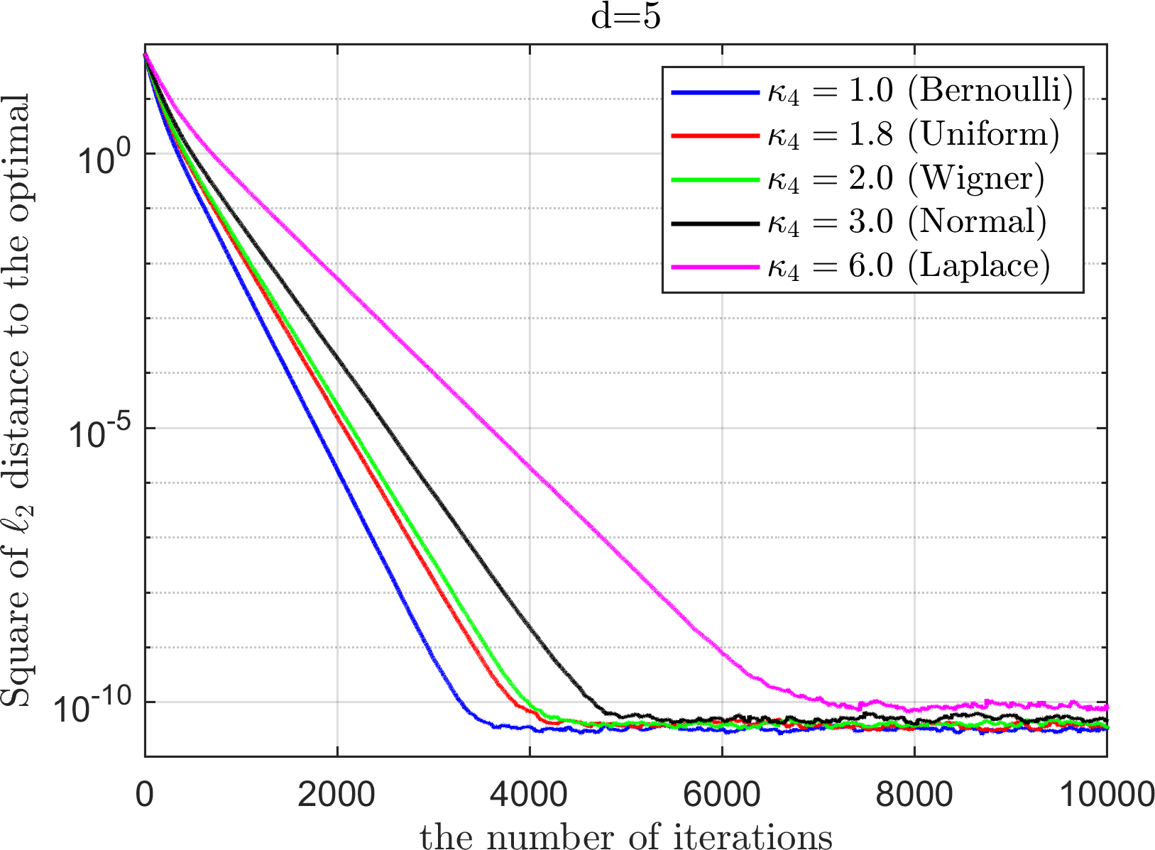
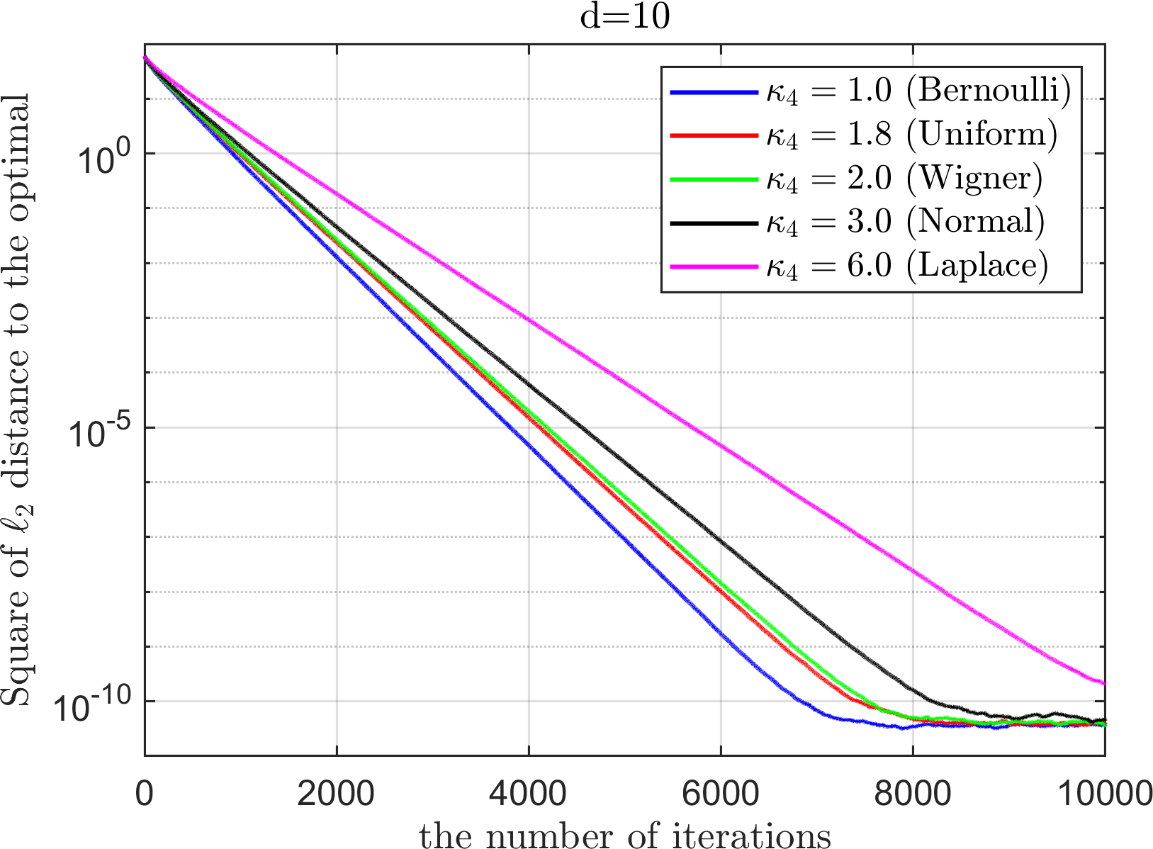
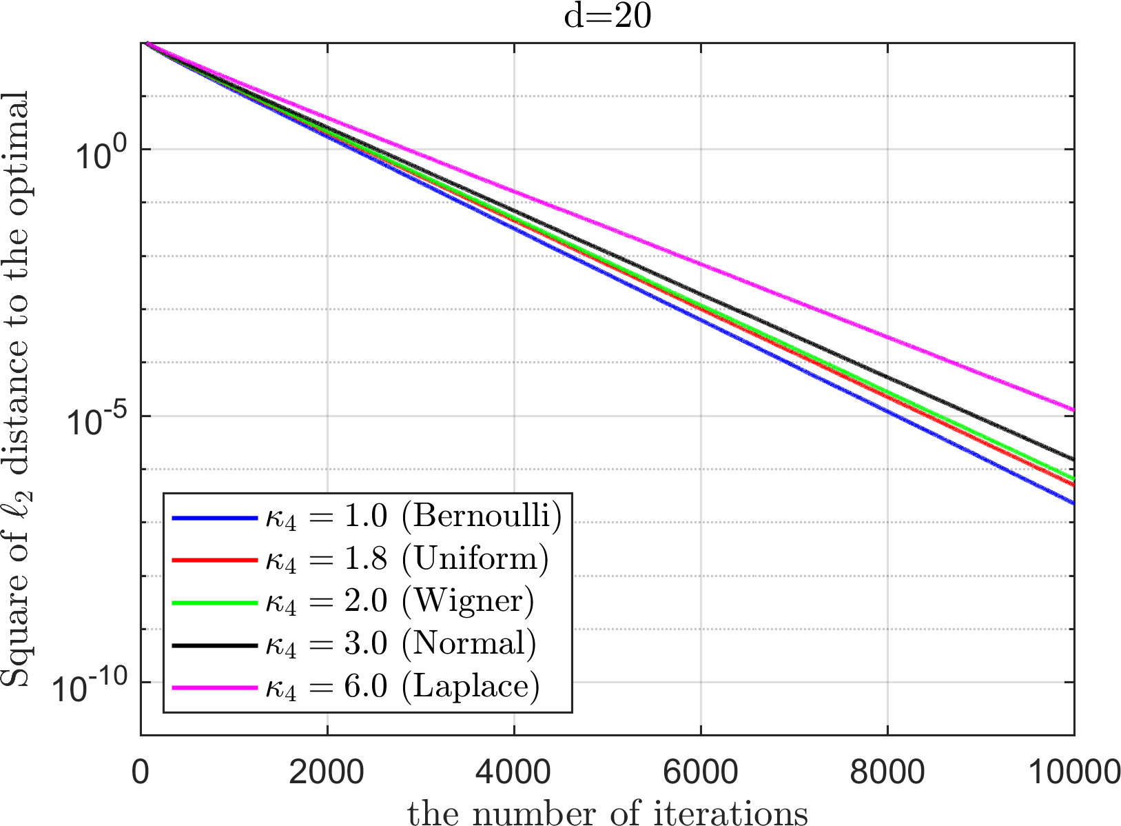
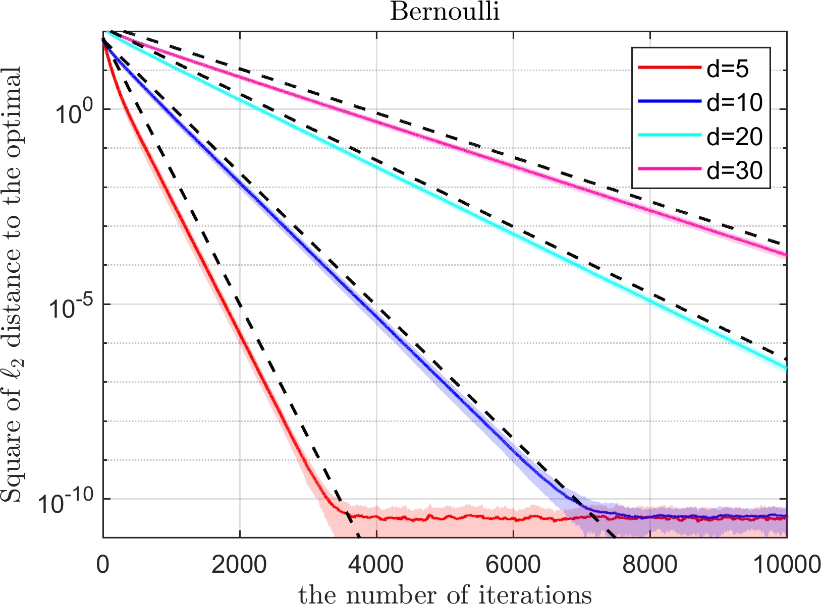
Figure 3: Top and bottom left: The averaged squared errors versus the number of iterations obtained by the RFG-based GD using the five different probability distributions at varying dimensions $d=5,10,20$. Bottom right: The averaged squared errors obtained by the Bernoulli RFG-based GD along with the upper bounds from Theorem 4.3 at varying dimensions $d=5,10,20,30$. The shaded area represents the area that falls within one standard deviation of the mean.

For RFG-based PHB, since an explicit optimal pair of $\mu$ and $\eta$ is not available from Theorem 4.5, we focus on the specialized case of $A$. As in the case of RFG-based GD, we generate a matrix $M$ and a vector $b$ randomly from the Gaussian distributions $\mathcal{N}(0,1)$ and $\mathcal{N}(5,1)$, respectively. We then perform the singular value decomposition (SVD) of $M$ to obtain $U,S,V$ matrices. We then set $S_{\text{new}}$ whose first two components are set to 1 and 10, and the remaining components are drawn independently from the uniform distribution on $(1,10)$. The newly reconstructed matrix is given by $A:=US_{\text{new}}$ whose condition number is exactly 10. Again, the data is generated once and fixed for all experiments. We remark that this allows us to find the best $\mu$ and $\eta$ from a grid search based on Proposition 4.7 for general probability distributions. The grid used for the search is

$$\Omega=\left\{(\mu,\eta):\mu=i\times 10^{-2},\eta=10^{-5+\frac{j}{100}},i\in\{-99,\dots,99\},j\in\{0,300\}\right\}.$$

which belongs to the domain $[-0.99,0.99]\times[10^{-5},10^{-2}]$. For any $(\mu,\eta)\in\Omega$, we calculate the largest eigenvalue of $\Phi^{10K}(I_{2d})$ according to Proposition 4.7 and choose the pair that gives the smallest value. On the left of Figure, the distribution of the largest eigenvalues of $\Phi^{10K}(I_{2d})$ is plotted on the grid $\Omega$. For the purpose of the visualization, we clipped the values to lie between $10^{-11}$ and $10^{0}$. The optimal pair found from the grid search is $(\mu^{*},\eta^{*})=(,)$. On the right of Figure, the sum of the consecutive squared errors, $\|\mathcal{E}_{k}\|^{2}$ defined in Theorem 4.5, is plotted with respect to the number of iterations. Again, the rate of convergence obtained from Theorem 4.5 is shown as a black dashed line, and the averaged error is shown as a black solid line.

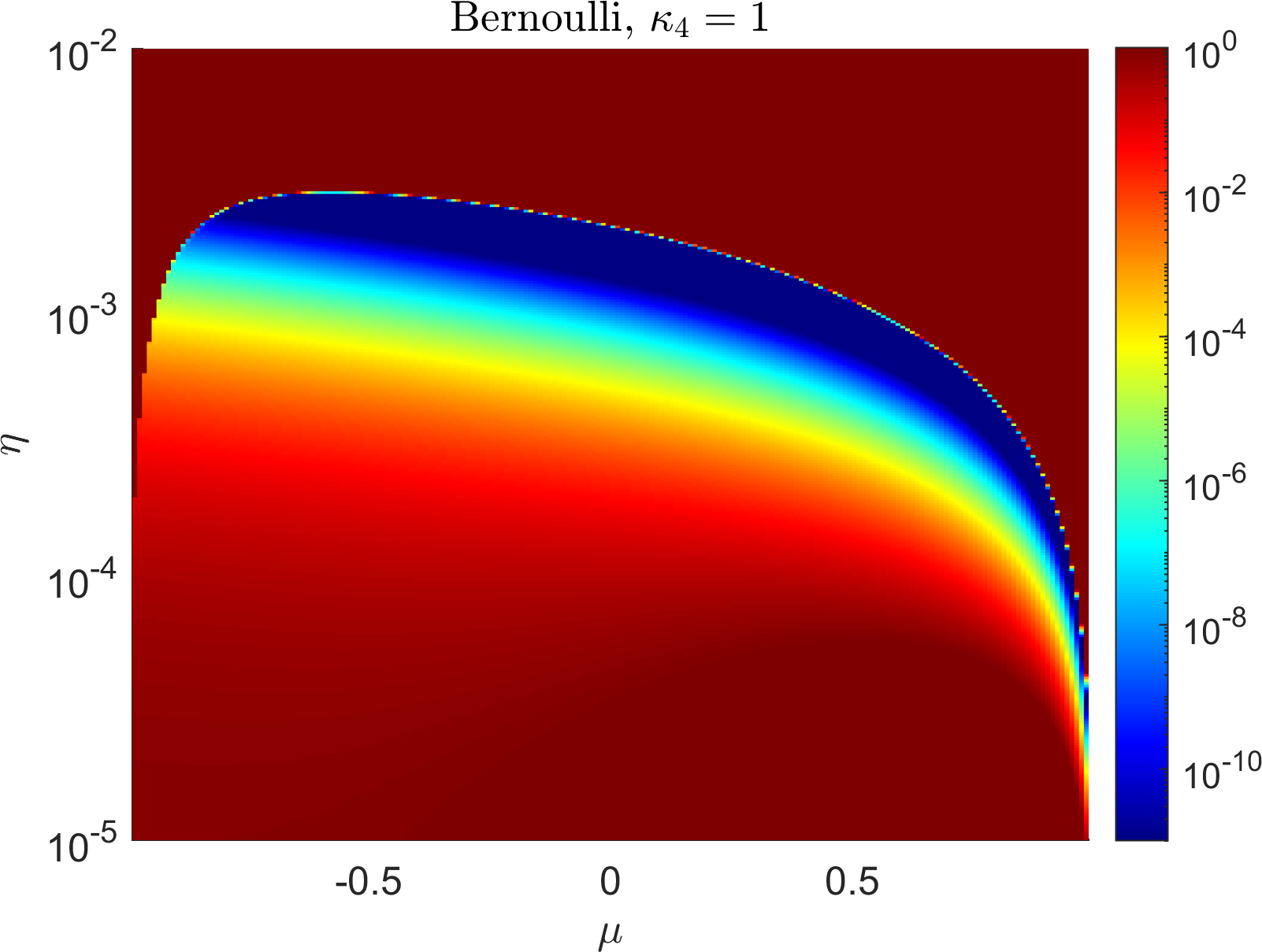
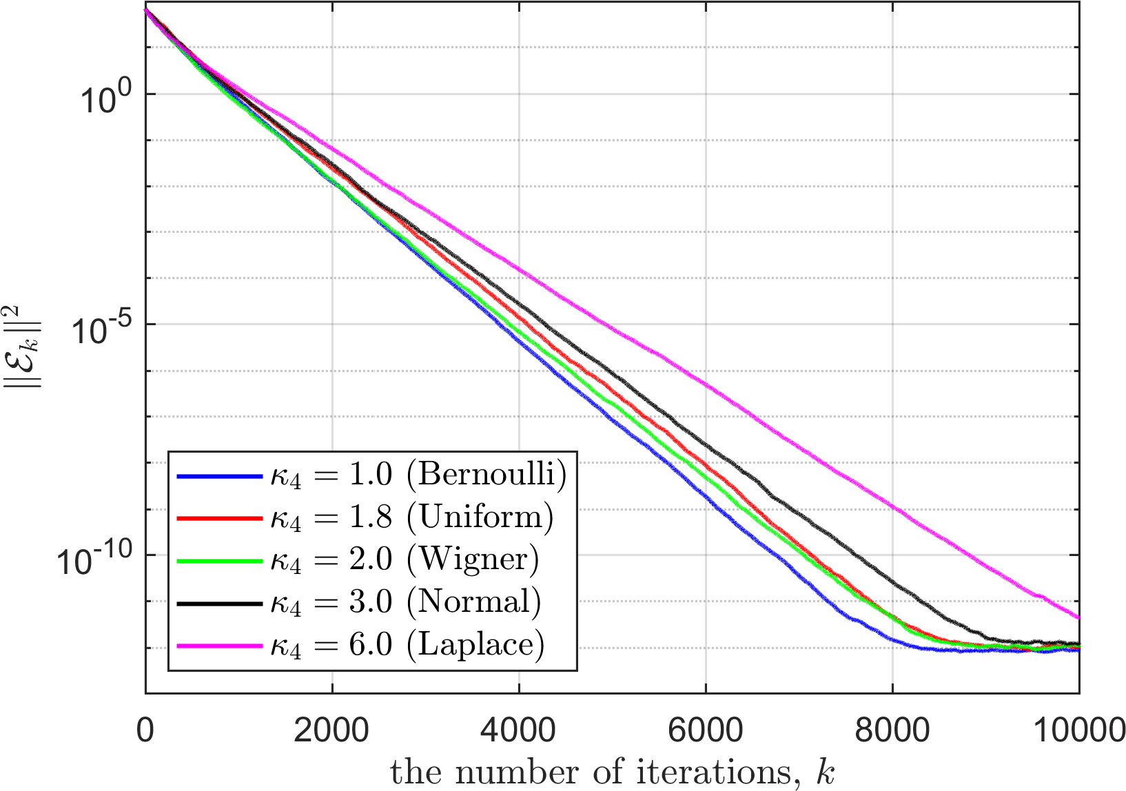
Figure 4: The value map of $\Phi^{10K}(I_{2d})$ on the grid $\Omega$ at $d=30$ for the Bernoulli distribution (left) and the Laplace distribution (middle). Right: The averaged squared errors versus the number of iterations obtained by the RFG-based PHB using the five different probability distributions at $d=30$.

5.2 Optimization test problems

We consider the non-quadratic objective functions from [10] that are popularly used as a testbed for optimization algorithms. In particular, the Rosenbrock and the Ackley functions are considered.

(13) $$\begin{split}\text{(Rosenbrock)}&\quad f_{\text{Ros}}(x_{1},x_{2})=100(x_{2}-x_{1}^{2})^{2}+(x_{1}-1)^{2},\\ \text{(Ackley)}&\quad f_{\text{Ack}}(x_{1},x_{2})=-20e^{0.5\sqrt{x_{1}^{2}+x_{2}^{2}}}-e^{\cos 2\pi x_{1}+\cos 2\pi x_{2}}+e+20.\end{split}$$

The global minima for the Rosenbrock and Ackley functions are $\textbf{x}^{*}=(1,1)$ and $\textbf{x}^{*}=(0,0)$, respectively. The initial starting point is set to $\textbf{x}^{(0)}=(0.5,0.5)$. For the Rosenbrock function, the learning rate scheduler is used with the initial rate of $10^{-1}$ with the decay rate of $0.1$ and the decay step of $25$. For the Ackley function, the learning rate is set to a constant of $2.4\times 10^{-3}$.

In Figure 5, the objective function values are reported with respect to the number of the RFG iterations. Similar to the previous example, the five different probability distributions are employed with the variance of $\frac{1}{d+\kappa_{4}-1}$. On the left and right, the results for the Rosenbrock and the Ackley are shown, respectively. It is clearly observed that the rates of convergence differ by the choice of probability distributions and in this case, the use of Bernoulli distribution results in the fastest convergence in both cases. In particular, for the Ackley case, the RFG with the Bernoulli distribution is the only one that successfully minimizes the objective function for all five independent simulations.

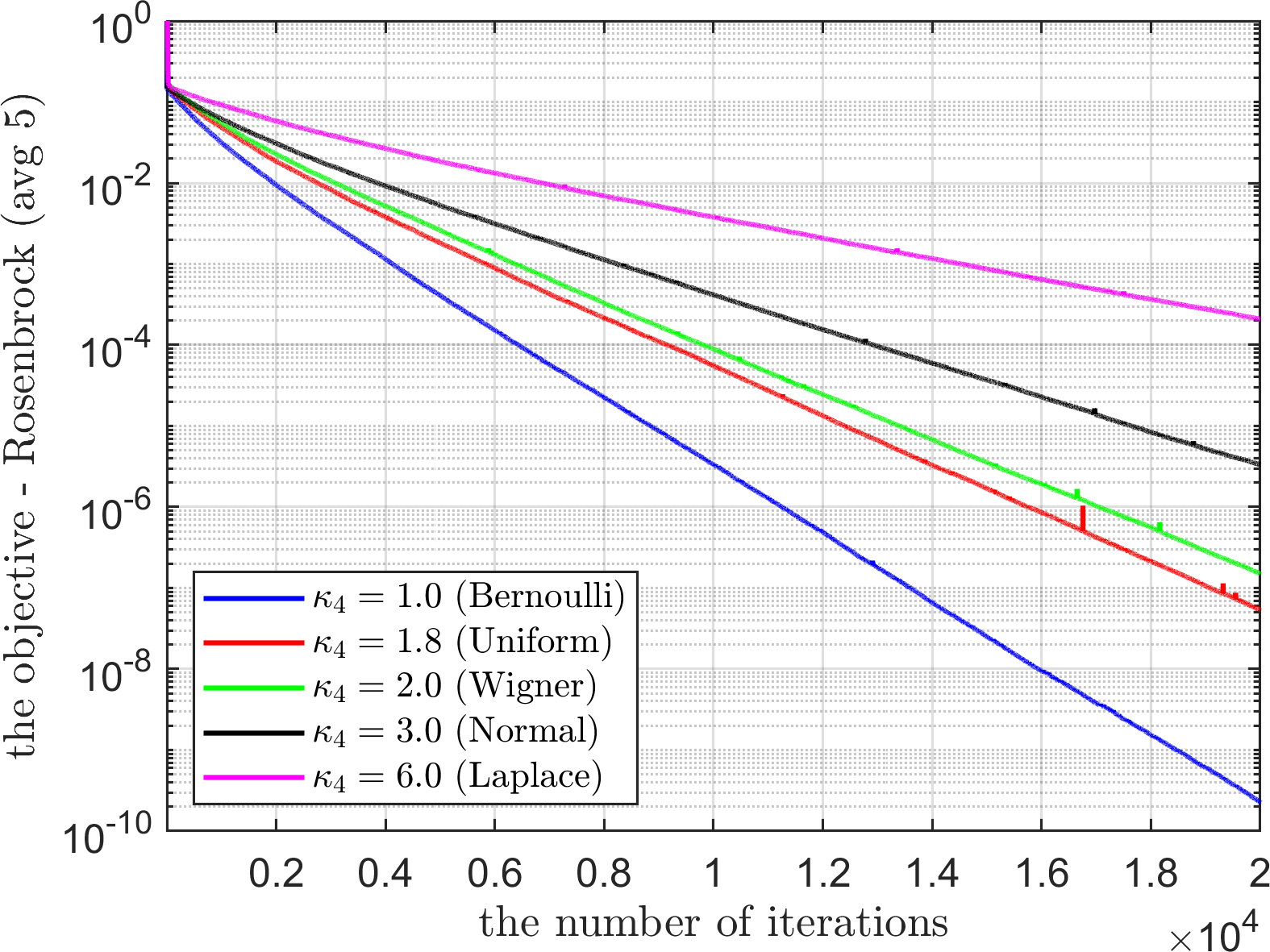
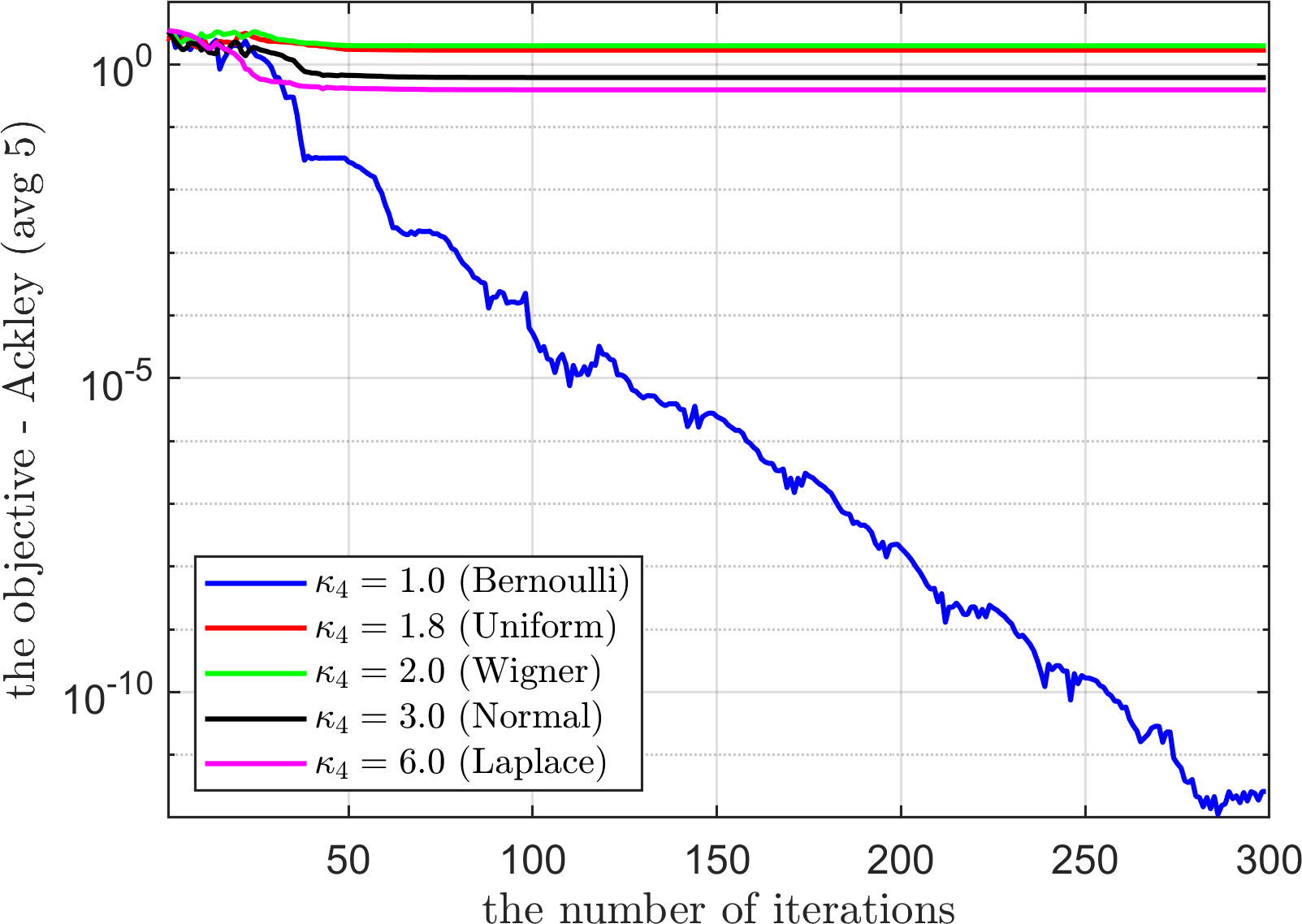
Figure 5: The objective function values versus the number of iterations by the RFG algorithms with five different probability distributions. The average of five independent simulations is reported. Left: The Rosenbrock function. Right: The Ackley function.

5.3 Scientific machine learning examples

In what follows, we demonstrate the performance of the RFG algorithm on the three scientific machine learning (SciML) applications – physics informed neural networks (PINNs), operator learning by deep operator networks (DeepONets) and function approximation. For this purpose, we briefly introduce the feed-forward neural network models. For $L\in\mathbb{N}_{\geq 2}$ and $N\in\mathbb{N}_{\geq 1}$, a $L$-layer feed-forward neural network (NN) of width $N$ is a function

$$u_{\text{NN}}(\cdot;\theta):\mathbb{R}^{d_{\text{in}}}\ni x\mapsto u^{L}(x)\in\mathbb{R}^{d_{\text{out}}},$$

where $u^{L}$ is defined recursively as follows: for $x\in\mathbb{R}^{d}$, let

$$u^{\ell}(x)=W^{\ell}\phi(u^{\ell-1}(x))+b^{\ell},\quad 2\leq\ell\leq L,$$

with $u^{1}(x)=W^{1}x+b^{1}$. Here $W^{\ell},b^{\ell}$ are the weight matrix and bias vector of the $\ell$-th hidden layer, and the collection $\theta=\{W^{\ell},b^{\ell}\}$ of them is called the network parameters. $\phi$ is an activation function that applies element-wise. Here $L$ and $N$ are referred to as the depth and width of the NN, which indicates the complexity of the deep NN.

1D Poisson equation by PINNs. Let us consider a learning task of solving the Poisson equation by the PINNs [11] with the RFG algorithm. Specifically, we consider

(14) $$-u^{\prime\prime}(x)=4\pi^{2}\sin(2\pi x),\quad\forall x\in(-1,1)\quad\text{with}\quad u(-1)=u(1)=0,$$

whose solution is given by $u(x)=\sin(2\pi x)$.

We employ a two-layer tanh NN, $u_{\text{NN}}$, of width 10, i.e., $L=2,N=10$, and train it to minimize the physics-informed loss function defined by

$$f_{\text{PINN}}(\theta)=\frac{1}{m}\sum_{i=1}^{m}\left(u^{\prime\prime}_{\text{NN}}(x_{i};\theta)+4\pi^{2}\sin(2\pi x_{i})\right)^{2}+\frac{1}{2}\left[\left(u_{\text{NN}}(-1;\theta)\right)^{2}+\left(u_{\text{NN}}(1;\theta)\right)^{2}\right],$$

where $x_{i}$’s are randomly uniformly sampled from $(-1,1)$. The goal is then to minimize $f_{\text{PINN}}$ on which we employ the RFG-based GD algorithm at varying probability distributions. The resulting NN is the approximated solution to the equation, namely, the PINN. The RFG-based GD algorithm is employed with a constant learning rate of $0.2$. The left of Figure 6 shows the relative $\ell_{2}$ errors of PINNs trained by the RFG-based GD algorithm with five different probability distributions. Notably, the Bernoulli distribution exhibits the fastest convergence while the normal distribution comes in second place. On the other hand, the uniform and Wigner distributions were unsuccessful, and the Laplace distribution diverged.

Learning an anti-derivative operator by DeepONets. Let us consider a simple ODE defined by $u^{\prime}=g$ in $(0,1)$ with $u(0)=0$. The corresponding solution operator is given by $G:g\mapsto u$ with $G[g](x)=\int_{0}^{x}g(s)ds$. The objective of the operator learning is to approximate $G$ using DeepONets. DeepONets [12] are an NN-based model for approximating nonlinear operators that consists of two subnetworks, namely, trunk and branch networks, which are $\mathbb{R}^{p}$-valued NNs. Let $t(\cdot;\theta_{t}),b(\cdot;\theta_{b})$ be the trunk and branch networks, respectively. A DeepONet is then constructed by $\mathcal{G}_{\text{NN}}[g](x)=\langle b(g;\theta_{b}),t(x;\theta_{t})\rangle$. Following [12], the training data is generated from a Gaussian random field with a spatial resolution of 100 grid points. See more details in [12]. Two-layer ReLU networks of width 40 are used for both the branch and trunk NNs. We employ the RFG-based GD algorithm with a constant learning rate of $0.1$. On the right of Figure 6, the relative $\ell_{2}$ errors are reported with respect to the number of iterations by the five probability distributions. It is seen that the normal and Bernoulli distributions perform similarly, while the other distributions fail to converge.

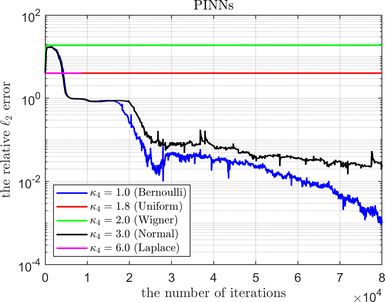
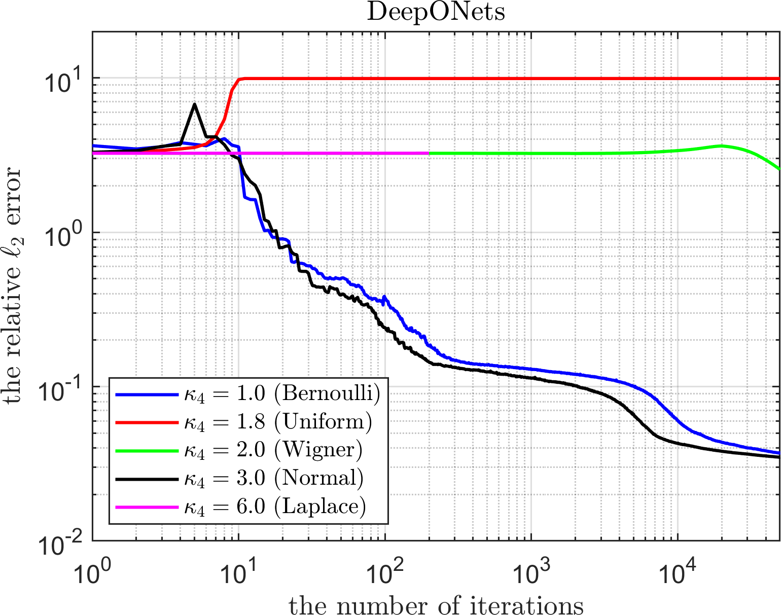
Figure 6: The training results of the RFG-based GD algorithms for the PINN (14) (left) and the DeepONet (right). The relative $\ell_{2}$ errors were reported with respect to the number of iterations.

Function approximation (FA). Let us consider a FA task, where the target function is $u(x)=\sin(2\pi x)\exp(-x^{2})$. Given a set of data points $\{x_{j}\}_{j=1}^{m}$, the loss function is defined by

(15) $$f_{\text{FA}}(\theta)=\frac{1}{m}\sum_{j=1}^{m}\left(u_{\text{NN}}(x_{j};\theta)-u(x_{j})\right)^{2}.$$

The learning goal is to minimize $f_{\text{FA}}$. A two-layer $\tanh$ NN of width 40 is employed. On the left of Figure 7, the training loss trajectories by GD and the RFG-based GD algorithm with the Bernoulli distribution were reported. It can be seen that RFG leads to a faster convergence when it is compared to GD. The right of Figure 7 depicts the NN final approximations by the two methods along with the target function.

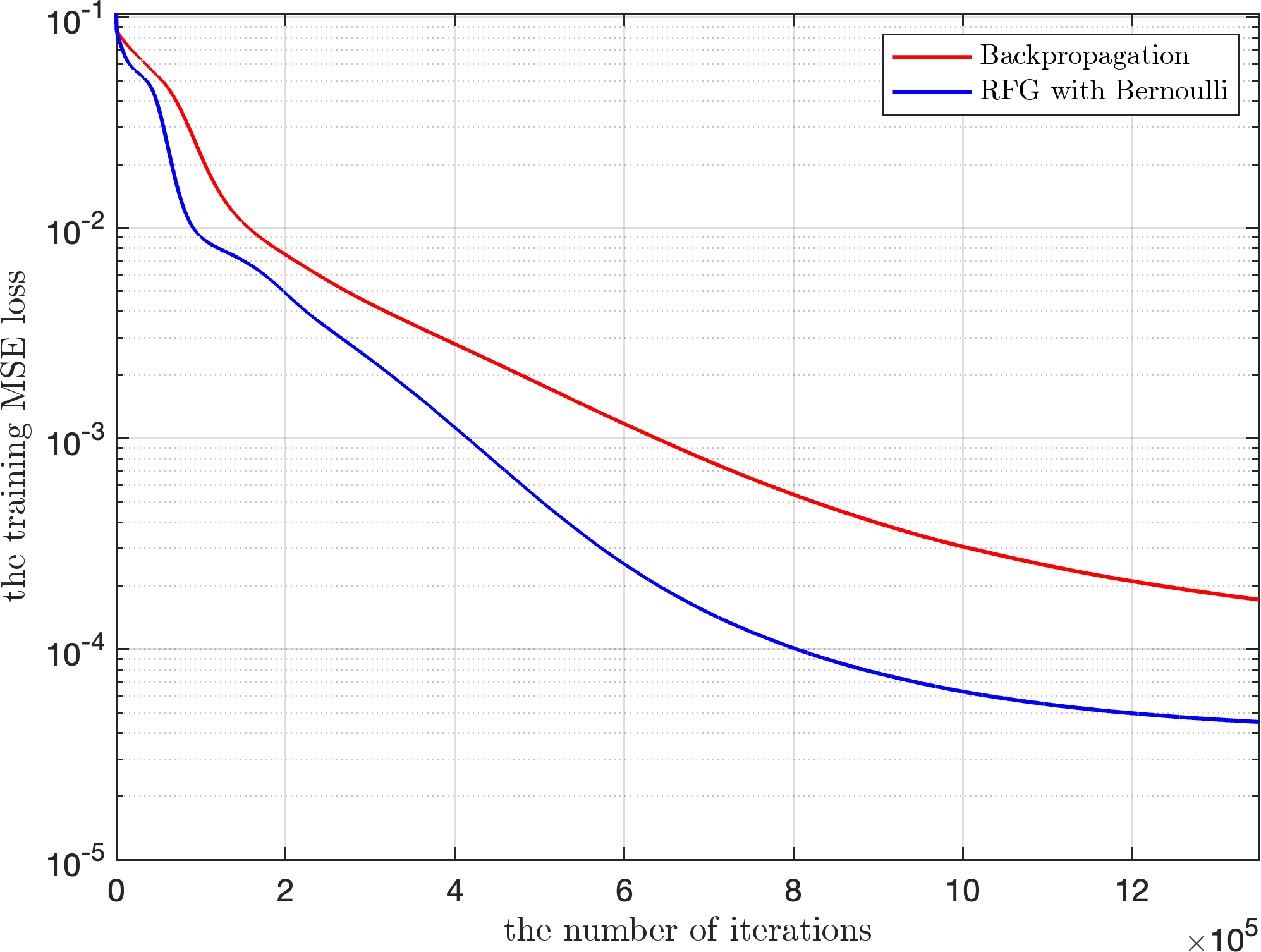
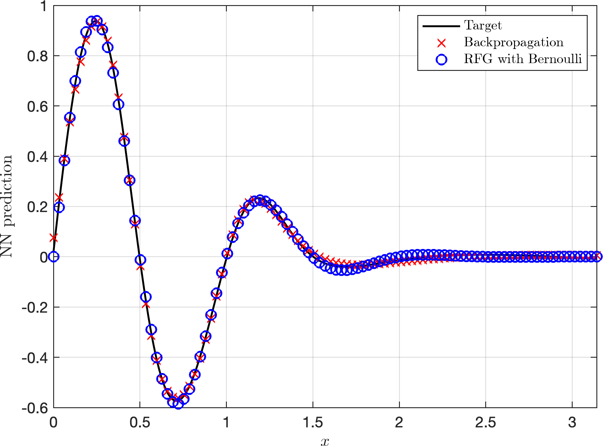
Figure 7: The function approximation results by backpropagation and the RFG. Left: The training loss trajectories by the standard GD with backpropagation and the RFG-based GD algorithm with the Bernoulli distribution. Right: The corresponding NN predictions along with the underlying target function (15)

5.4 Computational time comparison: RFG vs Backpropgation

We evaluate the computational time required for both backpropagation and the RFG method in the two problems -PINNs (14) and FA (15). The computational time is measured in terms of the number of iterations per second. Therefore, the larger the number, the better the computational efficiency. The measurements are performed by MacBookPro-2019 2.3 GHz 8-Core Intel Core i9 with 16 GB DDR memory.

We investigate the effect of the computational efficiency with respect to the NN complexity (width $N$ and depth $L$). The first set of experiments fixes the width as 200 and varies the depth from 4 to 8, while the second set fixes the depth as 4 and varies the width from 100 to 400. Table 2 summarizes all the results. $\Delta$% indicates the percentage increase of RFG with respect to BP. While no clear monotonic patterns manifest, we observe that RFG always yields higher numbers than BP, which illustrates a facet of the computation efficiency of RFG. Also, it is seen that the numbers for PINNs are smaller than those for FA. This is expected as the PINN loss requires partial derivatives which enforce reverse-mode AD. Consequently, the computational cost also rises [13], overshadowing some benefits gained from RFG.

the number of iterations per second
PINNs						Function Approx.
$N$	$L$	BP	RFG	$\Delta$%		$N$	$L$	BP	RFG	$\Delta$%
10	2	930	1030	11%
200	4	30	45	50%		200	4	80	120	50%
200	5	25	36	44%		200	5	62	92	48%
200	6	20	25	25%		200	6	47	70	49%
200	7	15	23	53%		200	7	42	60	43%
200	8	14	20	43%		200	8	35	48	37%
100	4	57	70	23%		100	4	160	270	69%
200	4	30	40	33%		200	4	70	140	100%
300	4	20	29	45%		300	4	50	81	62%
400	4	14	23	64%		400	4	35	45	29%
500	4	8	10	25%		500	4	28	32	14%

Table 2: A comparison of computational times, in terms of the number of iterations per second, for BP and RFG for the PINN (14) and the FA (15) tasks. Note that the larger the number, the better the efficiency.

6 Acknowledgements

K. Shukla gratefully acknowledges the support from the Air Force Office of Science and Research (AFOSR) under OSD/AFOSR MURI Grant FA9550-20-1-0358 and the Office of Naval Research (ONR) Vannevar Bush grant N00014-22-1-2795. Y. Shin was partially supported for this work by the NRF grant funded by the Ministry of Science and ICT of Korea (RS-2023-00219980).

Appendix A Proof of Theorem 3.6

Proof A.1.

Since $f$ is convex and $L$-strongly smooth, we have

$$\nabla_{\bm{z}}f(\bm{x})\leq\nabla_{\bm{z},h}f(\bm{x})\leq\nabla_{\bm{z}}f(\bm{x})+\frac{hL}{2}\|\bm{z}\|^{2}.$$

Let $\bm{z}=(z_{1},\dots,z_{d})^{\top}$ and observe that for any $j\in\{1,\dots,d\}$,

$$|\nabla_{\bm{z},h}f(\bm{x})z_{j}-\nabla_{\bm{z}}f(\bm{x})z_{j}|^{2}\leq\frac{h^{2}}{4}L^{2}\|\bm{z}\|^{4}|z_{j}|^{2}.$$

Since $z_{j}$’s are iid random variables whose first and third moments are zeros, we have

$$\mathbb{E}[\|\bm{z}\|^{4}|z_{j}|^{2}]=\sigma^{6}\left[\kappa_{6}+3(d-1)\kappa_{4}+(d-2)(d-1)\right],$$

where $\sigma^{2}=\mathbb{E}[Z^{2}]$ and $\kappa_{k}=\mathbb{E}[Z^{k}]/\sigma^{k}$. Hence, we have

$$\mathbb{E}\left[\|\nabla_{\bm{z},h}f(\bm{x})\bm{z}-\nabla_{\bm{z}}f(\bm{x})\bm{z}\|^{2}\right]\leq\frac{h^{2}}{4}L^{2}d\sigma^{6}\left(\kappa_{6}+(d-2+3\kappa_{4})(d-1)\right).$$

Also, observe that

$$|\nabla_{\bm{z}}f(\bm{x})z_{j}-(\nabla f(\bm{x}))_{j}|^{2} =|\nabla_{\bm{z}}f(\bm{x})|^{2}|z_{j}|^{2}+|(\nabla f(\bm{x}))_{j}|^{2}-2(\nabla f(\bm{x}))_{j}\nabla_{\bm{z}}f(\bm{x})z_{j}.$$

Thus we obtain

$$\mathbb{E}[|\nabla_{\bm{z}}f(\bm{x})z_{j}-(\nabla f(\bm{x}))_{j}|^{2}]=\sigma^{4}\|\nabla f(\bm{x})\|^{2}+(\sigma^{4}k_{4}-\sigma^{4}+1-2\sigma^{2})(\nabla f(\bm{x}))_{j}^{2},$$

which gives $\mathbb{E}\left[\|\nabla_{\bm{z}}f(\bm{x})\bm{z}-\nabla f(\bm{x})\|^{2}\right]=(\sigma^{4}(k_{4}+d-1)-2\sigma^{2}+1)\|\nabla f(\bm{x})\|^{2}$. Lastly, observe that

$$\mathbb{E}[|\langle\nabla_{\bm{z},h}^{\text{FM}}f(\bm{x})-\nabla_{\bm{z}}f(\bm{x})\bm{z},\nabla_{\bm{z}}f(\bm{x})\bm{z}-\nabla f(\bm{x})\rangle|]$$

$$\leq\mathbb{E}[|\nabla_{\bm{z},h}f(\bm{x})-\nabla_{\bm{z}}f(\bm{x})|(\|\bm{z}\|^{2}+1)\|\bm{z}\|\|\nabla f(\bm{x})\|]\leq\frac{hL}{2}\|\nabla f(\bm{x})\|\cdot\mathbb{E}[\|\bm{z}\|^{5}+\|\bm{z}\|^{3}].$$

We thus conclude that

$$\mathbb{E}\left[\|\nabla_{\bm{z},h}^{\text{FM}}f(\bm{x})-\nabla f(\bm{x})\|^{2}\right] \leq\frac{h^{2}}{2}L^{2}\sigma^{6}\left(\kappa_{6}+(d-2+3\kappa_{4})(d-1)\right)d$$

$$\qquad+hL\|\nabla f(\bm{x})\|\cdot\mathbb{E}[\|\bm{z}\|^{5}+\|\bm{z}\|^{3}]$$

$$\quad\qquad+(\sigma^{4}(d+k_{4}-1)+1-2\sigma^{2})\|\nabla f(\bm{x})\|^{2}.$$

Appendix B Useful Equalities

Lemma B.1.

Let $a,b\in\mathbb{R}^{d}$ and $A\in\mathbb{R}^{m\times d}$ whose $k,i$ component is denoted by $A_{k,i}$. Let $B$ be a diagonal matrix and $U$ be an orthogonal matrix. Suppose Assumption 4 holds. Then,

$$\mathbb{E}[|\langle a,\bm{z}\rangle|^{2}\|\bm{z}\|^{2}]=\sigma^{4}\left(\kappa_{4}+d-1\right)\|a\|^{2},$$

$$\mathbb{E}[|\langle a,\bm{z}\rangle|^{2}|\langle b,\bm{z}\rangle|^{2}\|\bm{z}\|^{2}]=\sigma^{6}\left[\alpha_{d}(\sum_{i=1}^{d}a_{i}^{2}b_{i}^{2})+\beta_{d}(\sum_{i\neq j}(a_{i}^{2}b_{j}^{2}+2a_{i}b_{i}a_{j}b_{j}))\right],$$

$$\mathbb{E}[\|A\bm{z}\|^{4}\|\bm{z}\|^{2}]=\sigma^{6}\sum_{k,l}\left[\alpha_{d}(\sum_{i=1}^{d}A_{k,i}^{2}A_{l,i}^{2})+\beta_{d}(\sum_{i\neq j}(A_{k,i}^{2}A_{l,j}^{2}+2A_{k,i}A_{l,i}A_{k,j}A_{l,j}))\right],$$

$$\mathbb{E}[Z\|BU^{\top}Z\|^{2}Z^{\top}]=\sigma^{4}\bigg{(}(\sum_{i=1}^{d}B_{i,i}^{2})I+(\kappa_{4}-1)\text{diag}(\langle U_{k,:}^{\circ 2},\text{diag}(B)^{\circ 2}\rangle)\bigg{)},$$

where $\alpha_{d}=\kappa_{6}+(d-1)\kappa_{4}$ and $\beta_{d}=d-2+2\kappa_{4}$.

Proof B.2.

For the first equality, note that $\mathbb{E}[z_{i}]=0$ and $\mathbb{E}[z_{i}z_{j}]=\sigma^{2}\delta_{ij}$. It then can be checked that

$$\mathbb{E}[\|\bm{z}\|^{2}|\langle a,\bm{z}\rangle|^{2}] =\mathbb{E}[\sum_{k}z_{k}^{2}\cdot\sum_{i,j}a_{i}a_{j}z_{i}z_{j}]=\sum_{k}\sum_{i,j}a_{i}a_{j}\mathbb{E}[z_{i}z_{j}z_{k}^{2}]$$

$$=\sum_{k}\left[a_{k}^{2}(\mathbb{E}[z^{4}]-\sigma^{4})+\sigma^{4}\|a\|^{2}\right]$$

$$=\left(\mathbb{E}[z^{4}]+(d-1)\sigma^{4}\right)\|a\|^{2}.$$

For the second equality, we categorize the index set $[d]^{4}=\{1,\dots,d\}^{4}$ by the following three cases:

$$\Omega_{1} =\{(i,j,k,l)\in[d]^{4}:i=j=k=l\},$$

$$\Omega_{2} =\{(i,j,k,l)\in[d]^{d}:i=j\neq k=l\text{ up to permutation}\},$$

$$\Omega_{3} =[d]^{4}\backslash(\Omega_{1}\cup\Omega_{2}).$$

Note that $|\Omega_{1}|=d$ and $|\Omega_{2}|=3d(d-1)$. It then can be checked that

$$(i,j,k,l)\in\Omega_{1} \implies\mathbb{E}[z_{i}z_{j}z_{k}z_{l}z_{1}^{2}]=\begin{cases}\sigma^{6}\kappa_{4}&\text{if }i\neq 1\\ \sigma^{6}\kappa_{6}&\text{if }i=1\end{cases},$$

$$(i,j,k,l)\in\Omega_{2} \implies\mathbb{E}[z_{i}z_{j}z_{k}z_{l}z_{1}^{2}]=\begin{cases}\sigma^{6}&\text{if }i\neq 1\text{ and }k\neq 1\\ \sigma^{6}\kappa_{4}&\text{if }i=1\text{ and }k\neq 1\\ \end{cases},$$

$$(i,j,k,l)\in\Omega_{3} \implies\mathbb{E}[z_{i}z_{j}z_{k}z_{l}z_{1}^{2}]=0.$$

Observe that since $|\langle a,\bm{z}\rangle|^{2}|\langle b,\bm{z}\rangle|^{2}=\sum_{i,j}a_{i}a_{j}z_{i}z_{j}\cdot\sum_{k,l}b_{k}b_{l}z_{k}z_{l}$, we have

$$|\langle a,\bm{z}\rangle|^{2}|\langle b,\bm{z}\rangle|^{2}$$

$$=\sum_{(i,j,k,l)\in\Omega_{1}}+\sum_{(i,j,k,l)\in\Omega_{2}}+\sum_{(i,j,k,l)\in\Omega_{3}}a_{i}a_{j}b_{k}b_{l}z_{i}z_{j}z_{k}z_{l}$$

$$=\sum_{i=1}^{d}a_{i}^{2}b_{i}^{2}z_{i}^{4}+\sum_{i\neq j}(a_{i}^{2}b_{j}^{2}+2a_{i}b_{i}a_{j}b_{j})z_{i}^{2}z_{j}^{2}+\sum_{(i,j,k,l)\in\Omega_{3}}a_{i}a_{j}b_{k}b_{l}z_{i}z_{j}z_{k}z_{l}.$$

Thus,

$$\mathbb{E}[|\langle a,\bm{z}\rangle|^{2}|\langle b,\bm{z}\rangle|^{2}z_{1}^{2}]$$

$$=\sigma^{6}\kappa_{4}(\sum_{i=1}^{d}a_{i}^{2}b_{i}^{2})+\sigma^{6}(\kappa_{6}-\kappa_{4})a_{1}^{2}b_{1}^{2}+\sigma^{6}\sum_{i\neq j}(a_{i}^{2}b_{j}^{2}+2a_{i}b_{i}a_{j}b_{j})$$

$$\quad+\sigma^{6}(\kappa_{4}-1)\sum_{j\neq 1}(a_{1}^{2}b_{j}^{2}+2a_{1}b_{1}a_{j}b_{j})+\sigma^{6}(\kappa_{4}-1)\sum_{i\neq 1}(a_{i}^{2}b_{1}^{2}+2a_{i}b_{i}a_{1}b_{1}),$$

which gives

$$\mathbb{E}[|\langle a,\bm{z}\rangle|^{2}|\langle b,\bm{z}\rangle|^{2}\|\bm{z}\|^{2}]$$

$$=\sigma^{6}\left[(\kappa_{6}+(d-1)\kappa_{4})(\sum_{i=1}^{d}a_{i}^{2}b_{i}^{2})+(d-2+2\kappa_{4})(\sum_{i\neq j}(a_{i}^{2}b_{j}^{2}+2a_{i}b_{i}a_{j}b_{j}))\right].$$

For the third equality, let $\alpha_{d}=\kappa_{6}+(d-1)\kappa_{4}$ and $\beta_{d}=d-2+2\kappa_{4}$. By applying the second equality, we obtain

$$\mathbb{E}[\|A\bm{z}\|^{4}\|\bm{z}\|^{2}]=\mathbb{E}[(\sum_{k=1}^{m}|\langle A_{k,:},\bm{z}\rangle|^{2})^{2}\|\bm{z}\|^{2}]=\sum_{k,l}\mathbb{E}[|\langle A_{k,:},\bm{z}\rangle|^{2}|\langle A_{l,:},\bm{z}\rangle|^{2}\|\bm{z}\|^{2}]$$

$$=\sigma^{6}\sum_{k,l}\left[\alpha_{d}(\sum_{i=1}^{d}A_{k,i}^{2}A_{l,i}^{2})+\beta_{d}(\sum_{i\neq j}(A_{k,i}^{2}A_{l,j}^{2}+2A_{k,i}A_{l,i}A_{k,j}A_{l,j}))\right].$$

For the fourth equality, let $B_{:,i}$ and $B_{k,:}$ be the $i$-th column and the $k$-th row of $B$, respectively. Observe that for any $k$,

$$\mathbb{E}[\|B^{\top}\bm{z}\|^{2}z_{k}^{2}] =\sum_{i=1}^{d}\mathbb{E}[|\langle B_{:,i},\bm{z}\rangle|^{2}z_{k}^{2}]=\sum_{i=1}^{d}[B_{k,i}^{2}(\mathbb{E}[z^{4}]-\sigma^{4})+\sigma^{4}\|B_{:,i}\|^{2}]$$

$$=\sigma^{4}(\kappa_{4}-1)\|B_{k,:}\|^{2}+\sigma^{4}\|B\|_{F}^{2}$$

Thus, $\mathbb{E}[\bm{z}\|B^{\top}\bm{z}\|^{2}\bm{z}^{\top}]=\sigma^{4}\left(\|B\|_{F}^{2}I+(\kappa_{4}-1)\text{diag}(\|B_{k,:}\|^{2})\right)$.

Appendix C Proof of Theorem 4.3

Proof C.1.

Observe that

$$\bm{x}^{(k+1)} =\bm{x}^{(k)}-\eta\left(\frac{f(\bm{x}^{(k)}+h\bm{z})-f(\bm{x}^{(k)})}{h}\right)\bm{z}$$

$$=\bm{x}^{(k)}-\eta\bm{z}\bm{z}^{\top}\left(A^{\top}(A\bm{x}^{(k)}-b)\right)-\eta\frac{h}{2}\|A\bm{z}\|^{2}\bm{z}.$$

Let $\epsilon^{(k)}=\bm{x}^{(k)}-\bm{x}^{*}$ where $\bm{x}^{*}=(A^{\top}A)^{-1}A^{\top}b$. Then,

$$\epsilon^{(k+1)} =(I-\eta\bm{z}\bm{z}^{\top}A^{\top}A)\epsilon^{(k)}-\frac{h\eta}{2}\|A\bm{z}\|^{2}\bm{z},$$

$$\|\epsilon^{(k+1)}\|^{2} =\|P_{\bm{z}}^{A}(\eta)\epsilon^{(k)}\|^{2}+\frac{h^{2}\eta^{2}}{4}\|A\bm{z}\|^{4}\|\bm{z}\|^{2}-h\eta\|A\bm{z}\|^{2}\langle\bm{z},P_{\bm{z}}^{A}(\eta)\epsilon^{(k)}\rangle,$$

where $P_{\bm{z}}^{A}(\eta):=I-\eta\bm{z}\bm{z}^{\top}A^{\top}A$.

Let $\bm{z}=(z_{1},\dots,z_{d})^{\top}$ be a random vector satisfying Assumption 4. It then can be checked (also from Lemma B.1) that $\mathbb{E}[\bm{z}\bm{z}^{\top}]=\sigma^{2}I$ and $\mathbb{E}[\|\bm{z}\|^{2}\bm{z}\bm{z}^{\top}]=\gamma_{d}I$ where $\gamma_{d}=\sigma^{4}(\kappa_{4}+(d-1))$. We then have

$$\mathbb{E}[P_{\bm{z}}^{A}(\eta)^{\top}P_{\bm{z}}^{A}(\eta)] =I-2\eta\sigma^{2}A^{\top}A+\eta^{2}\gamma_{d}A^{\top}AA^{\top}A$$

$$=(1-\frac{\sigma^{4}}{\gamma_{d}})I+\big{(}\frac{\sigma^{2}}{\sqrt{\gamma_{d}}}I-\eta\sqrt{\gamma_{d}}A^{\top}A\big{)}^{2},$$

which gives $\mathbb{E}[\|P_{\bm{z}}^{A}(\eta)\epsilon^{(k)}\|^{2}]=(1-\frac{\sigma^{4}}{\gamma_{d}})\|\epsilon^{(k)}\|^{2}+\|\big{(}\frac{\sigma^{2}}{\sqrt{\gamma_{d}}}I-\eta\sqrt{\gamma_{d}}A^{\top}A\big{)}\epsilon^{(k)}\|^{2}$. Since the 1st, 3rd, and 5th moments are zeros, $\mathbb{E}[\|A\bm{z}\|^{2}\langle\bm{z},P_{\bm{z}}^{A}(\eta)\epsilon^{(k)}\rangle]=0$.

Let $\lambda_{\min}=\lambda_{1}\leq\lambda_{2}\leq\cdots\leq\lambda_{d}=\lambda_{\max}$ be eigenvalues of $A^{\top}A$ and $q_{1},\dots,q_{d}$ be the corresponding eigenvectors. Then, since $\sigma^{4}/\gamma_{d}=1/(\kappa_{4}+d-1)$, we have

$$\mathbb{E}[\|\epsilon^{(k+1)}\|^{2}]-\frac{\eta^{2}h^{2}}{4}\sigma^{6}\mathcal{F}(d,\kappa_{4},\kappa_{6},A)$$

$$=\sum_{i=1}^{d}\left(1-\frac{1}{\kappa_{4}+d-1}+(\frac{1}{\sqrt{\kappa_{4}+d-1}}-\eta\sqrt{\kappa_{4}+d-1}\sigma^{2}\lambda_{i})^{2}\right)|\langle\epsilon^{(k)},q_{i}\rangle|^{2},$$

where $\mathcal{F}(d,\kappa_{4},\kappa_{6},A)$ is defined in Proposition 4.1. If $\eta=\frac{1}{\frac{\lambda_{\max}+\lambda_{\min}}{2}(\kappa_{4}+d-1)\sigma^{2}}$,

$$\mathbb{E}[\|\epsilon^{(k+1)}\|^{2}]$$

$$\leq\left(1-\frac{1}{\kappa_{4}+d-1}\left[1-(\frac{\kappa_{A}-1}{\kappa_{A}+1})^{2}\right]\right)\|\epsilon^{(k)}\|^{2}+\frac{h^{2}\sigma^{2}\mathcal{F}(d,\kappa_{4},\kappa_{6},A)}{(\frac{\lambda_{\max}+\lambda_{\min}}{2})^{2}(\kappa_{4}+d-1)^{2}},$$

where $\kappa_{A}=\frac{\lambda_{\max}}{\lambda_{\min}}$. By letting $r_{\text{rate}}:=1-\frac{1}{\kappa_{4}+d-1}\left[1-(\frac{\kappa_{A}-1}{\kappa_{A}+1})^{2}\right]$ and recursively applying the above inequality, the desired result is obtained.

Appendix D Proof of Theorem 4.5

Proof D.1.

Let $\epsilon_{k+1}=\bm{x}^{(k+1)}-\bm{x}^{*}$. It then follows from the update rule (10) of the RFG-based PHB method that

$$\epsilon_{k+1} =\epsilon_{k}-\eta\nabla_{\bm{z},h}^{\text{FM}}f(\bm{x}^{(k)})+\mu(\epsilon_{k}-\epsilon_{k-1})$$

$$=((1+\mu)I-\eta\bm{z}\bm{z}^{\top}A^{\top}A)\epsilon_{k}-\mu\epsilon_{k-1}-\eta\frac{h}{2}\|A\bm{z}\|^{2}\bm{z},$$

which can be equivalently written as $\mathcal{E}_{k+1}=\bm{M}\mathcal{E}_{k}+\bm{\alpha}$ where

$$\bm{M}=\begin{pmatrix}(1+\mu)I-\eta\bm{z}\bm{z}^{\top}A^{\top}A&-\mu I\\ I&0\end{pmatrix},\quad\bm{\alpha}=-\eta\frac{h}{2}\|A\bm{z}\|^{2}\begin{pmatrix}\bm{z}\\ 0\end{pmatrix}.$$

Note that it can be checked that $\bm{M}=\bm{U}\overline{\bm{M}}\bm{U}^{\top}$ where

(16) $$\overline{\bm{M}}=\begin{pmatrix}(1+\mu)I-\eta U_{A}^{\top}\bm{z}\bm{z}^{\top}U_{A}\Sigma_{A}&-\mu I\\ I&0\end{pmatrix}.$$

Let $\tilde{\mathcal{E}}_{k}=\bm{U}^{\top}\mathcal{E}_{k}$ and $\tilde{\bm{\alpha}}=\bm{U}^{\top}\bm{\alpha}$. Then, we have

(17) $$\tilde{\mathcal{E}}_{k+1}=\overline{\bm{M}}\tilde{\mathcal{E}}_{k}+\tilde{\bm{\alpha}}.$$

Also, observe that $\|\mathcal{E}_{k+1}\|^{2}=\|\overline{\bm{M}}\tilde{\mathcal{E}}_{k}\|^{2}+2\langle\overline{\bm{M}}\tilde{\mathcal{E}}_{k},\tilde{\bm{\alpha}}\rangle+\|\tilde{\bm{\alpha}}\|^{2}$. Since $\bm{z}$ satisfies Assumption 4, it can be checked that $\mathbb{E}[\langle\overline{\bm{M}}\tilde{\mathcal{E}}_{k},\tilde{\bm{\alpha}}\rangle]=0$ where the expectation is taken with respect to $\bm{z}$. From this, we obtain $\mathbb{E}[\|\mathcal{E}_{k+1}\|^{2}]=\mathbb{E}[\|\overline{\bm{M}}\tilde{\mathcal{E}}_{k}\|^{2}]+\mathbb{E}[\|\tilde{\bm{\alpha}}\|^{2}]$. It follows from Lemma D.2 that we have $\mathbb{E}[\|\mathcal{E}_{k+1}\|^{2}]=\tilde{\mathcal{E}}_{k}^{\top}\Phi_{A,\mu,\rho,\sigma^{2}}(I_{2d})\tilde{\mathcal{E}}_{k}+\mathbb{E}[\|\tilde{\bm{\alpha}}\|^{2}]$. With (17), we have

$$\mathbb{E}[\|\mathcal{E}_{k+1}\|^{2}] =\tilde{\mathcal{E}}_{k-1}^{\top}\mathbb{E}_{k-1}[\overline{\bm{M}}^{\top}\Phi(I_{2d})\overline{\bm{M}}]\tilde{\mathcal{E}}_{k-1}+\mathbb{E}[\|\tilde{\bm{\alpha}}\|^{2}_{\Phi}]+\mathbb{E}[\|\tilde{\bm{\alpha}}\|^{2}]$$

$$=\tilde{\mathcal{E}}_{k-1}^{\top}\Phi^{2}(I_{2d})\tilde{\mathcal{E}}_{k-1}+\mathbb{E}[\|\tilde{\bm{\alpha}}\|^{2}_{\Phi}]+\mathbb{E}[\|\tilde{\bm{\alpha}}\|^{2}]$$

where the expectation over the random variables used in the $(k-1)$th iteration. By repeating the above recursion, we have $\mathbb{E}[\|\tilde{\mathcal{E}}_{k}\|^{2}]=\tilde{\mathcal{E}}_{0}^{\top}\Phi^{k}(I_{2d})\tilde{\mathcal{E}}_{0}+\sum_{i=0}^{k-1}\mathbb{E}[\|\tilde{\bm{\alpha}}\|^{2}_{\Phi^{i}}]$ and the proof is completed.

Lemma D.2.

Let $\bm{S}=\begin{bmatrix}S_{1}&S_{2}^{\top}\\ S_{2}&S_{3}\end{bmatrix}\in\text{Sym}_{2d}$. Then, $\mathbb{E}[\overline{\bm{M}}^{\top}\bm{S}\overline{\bm{M}}]=\begin{bmatrix}H_{1}&H_{2}^{\top}\\ H_{2}&H_{3}\end{bmatrix}$ where $H_{i}$’s are defined in (11) and $\overline{\bm{M}}$ is defined in (16).

Proof D.3 (Proof of Lemma D.2).

Let $J=(1+\mu)I-\eta U_{A}^{\top}zz^{\top}U_{A}\Sigma_{A}$. Since $\mathbb{E}[\bm{z}\bm{z}^{\top}]=\sigma^{2}I$, we have $V:=\mathbb{E}[J]=(1+\mu)I-\eta\sigma^{2}\Sigma_{A}$. We then have

$$\mathbb{E}[\overline{\bm{M}}^{\top}\bm{S}\overline{\bm{M}}] =\mathbb{E}[\begin{bmatrix}J^{\top}&I\\ -\mu I&0\end{bmatrix}\begin{bmatrix}S_{1}&S_{2}\\ S_{2}&S_{3}\end{bmatrix}\begin{bmatrix}J&-\mu I\\ I&0\end{bmatrix}]$$

$$=\begin{bmatrix}\mathbb{E}[J^{\top}S_{1}J]+2S_{2}V+S_{3}&-\mu(V^{\top}S_{1}+S_{2})\\ -\mu(S_{1}V+S_{2})&\mu^{2}S_{1}\end{bmatrix}.$$

Since $S_{1}$ is diagonal, it follows from Lemma B.1 that

$$\mathbb{E}[J^{\top}S_{1}J]$$

$$=\mathbb{E}[((1+\mu)I-\eta\Sigma_{A}U_{A}^{\top}\bm{z}\bm{z}^{\top}U_{A})S_{1}((1+\mu)I-\eta U_{A}^{\top}\bm{z}\bm{z}^{\top}U_{A}\Sigma_{A})]$$

$$=(1+\mu)^{2}S_{1}-(1+\mu)\eta\sigma^{2}(\Sigma_{A}S_{1}+S_{1}\Sigma_{A})+\eta^{2}\Sigma_{A}U_{A}^{\top}\mathbb{E}[\bm{z}\|(U_{A}L_{1})^{\top}\bm{z}\|^{2}\bm{z}^{\top}]U_{A}\Sigma_{A}$$

$$=(1+\mu)^{2}S_{1}-(1+\mu)\eta\sigma^{2}(\Sigma_{A}S_{1}+S_{1}\Sigma_{A})+(\eta\sigma^{2})^{2}(U_{A}\Sigma_{A})^{\top}H_{4}U_{A}\Sigma_{A},$$

where $S_{1}=L_{1}L_{1}^{\top}$ is the Cholesky decomposition of $S_{1}$ and

$$H_{4}=\sigma^{4}\|U_{A}L_{1}\|_{F}^{2}I+(\kappa_{4}-1)\sigma^{4}\text{diag}(\|(U_{A}L_{1})_{k,:}\|^{2}).$$

References

- [1] A. G. Baydin, B. A. Pearlmutter, A. A. Radul, and J. M. Siskind, Automatic differentiation in machine learning: a survey, J. Mach. Learn. Res., 18 (2018), pp. 1–43.
- [2] I. Dunning, J. Huchette, and M. Lubin, JuMP: A modeling language for mathematical optimization, SIAM review, 59 (2017), pp. 295–320.
- [3] M. Innes, A. Edelman, K. Fischer, C. Rackauckas, E. Saba, V. B. Shah, and W. Tebbutt, A differentiable programming system to bridge machine learning and scientific computing, preprint arXiv:1907.07587, (2019).
- [4] G. E. Karniadakis, I. G. Kevrekidis, L. Lu, P. Perdikaris, S. Wang, and L. Yang, Physics-informed machine learning, Nat. Rev. Phys., 3 (2021), pp. 422–440.
- [5] T. P. Lillicrap, A. Santoro, L. Marris, C. J. Akerman, and G. Hinton, Backpropagation and the brain, Nat. Rev. Neurosci., 21 (2020), pp. 335–346.
- [6] G. Hinton, The forward-forward algorithm: Some preliminary investigations, preprint arXiv:2212.13345, (2022).
- [7] B. Scellier and Y. Bengio, Equilibrium propagation: Bridging the gap between energy-based models and backpropagation, Front. Comput. Neurosci., 11 (2017), p. 24.
- [8] A. G. Baydin, B. A. Pearlmutter, D. Syme, F. Wood, and P. Torr, Gradients without backpropagation, preprint arXiv:2202.08587, (2022).
- [9] J. Bradbury, R. Frostig, P. Hawkins, M. J. Johnson, C. Leary, D. Maclaurin, G. Necula, A. Paszke, J. VanderPlas, S. Wanderman-Milne, and Q. Zhang, JAX: composable transformations of Python+NumPy programs, 2018, http://github.com/google/jax.
- [10] S. Surjanovic and D. Bingham, Virtual library of simulation experiments: Test functions and datasets. Retrieved September 26, 2023, from http://www.sfu.ca/~ssurjano.
- [11] M. Raissi, P. Perdikaris, and G. E. Karniadakis, Physics-informed neural networks: A deep learning framework for solving forward and inverse problems involving nonlinear partial differential equations, J. Comput. Phys., 378 (2019), pp. 686–707.
- [12] L. Lu, P. Jin, G. Pang, Z. Zhang, and G. E. Karniadakis, Learning nonlinear operators via DeepONet based on the universal approximation theorem of operators, Nat. Mach. Intell., 3 (2021), pp. 218–229.
- [13] K. Shukla, A. D. Jagtap, and G. E. Karniadakis, Parallel physics-informed neural networks via domain decomposition, J. Comput. Phys., 447 (2021), p. 110683.