Abstract

Contextual bandit algorithms are at the core of many applications, including recommender systems, clinical trials, and optimal portfolio selection. One of the most popular problems studied in the contextual bandit literature is to maximize the sum of the rewards in each round by ensuring a sublinear regret against the best-fixed context-dependent policy. However, in many applications, the cumulative reward is not the right objective - the bandit algorithm must be fair in order to avoid the echo-chamber effect and comply with the regulatory requirements. In this paper, we consider the $\alpha$-Fair Contextual Bandits problem, where the objective is to maximize the global $\alpha$-fair utility function - a non-decreasing concave function of the cumulative rewards in the adversarial setting. The problem is challenging due to the non-separability of the objective across rounds. We design an efficient algorithm that guarantees an approximately sublinear regret in the full-information and bandit feedback settings.

1 Introduction and related work

In applications such as personalized recommendations, greedily optimizing for the most relevant content for each user profile tends to reduce the diversity of the recommended items as it induces an unhealthy echo-chamber effect and propagates systematic biases (Celis et al., 2019). Recall that standard contextual bandits with a separable cumulative utility function tend to maximize the click-through rates (CTR) by recommending the most popular item for each user profile (Semenov et al., 2022). However, an over-emphasis on the CTR metric invariably leads to polarization of opinions. A similar fairness issue arises with other popular recommender systems, such as movie or song recommendations by Netflix and Spotify and various online job recommendation portals. The main objective of this paper is to design a class of fair contextual bandit algorithms equipped with a quantifiable fairness guarantee that holds even in the adversarial setting. Towards this goal, we propose a contextual bandit algorithm that maximizes the non-linear $\alpha$-fair utility function instead of the usual time-separable utility function. Due to the diminishing return property, the optimizer of the concave $\alpha$-fair utility function strikes a trade-off between the fairness and the accuracy of the recommendations through a tunable hyperparameter $\alpha\in[0,1).$ Lan et al. (2010) gave an axiomatic characterization of fair utility functions and showed that the $\alpha$-fair utility function comes out naturally. Other standard utility functions, e.g., proportional fair and min-max utilities, can be shown to be a limiting form of the $\alpha$-fair utility.

Fairness in bandit and online convex optimization have been extensively studied in the literature (Joseph et al., 2016; Chen et al., 2020; Agarwal et al., 2014; Patil et al., 2021; Si Salem et al., 2022; Even-Dar et al., 2009; Claure et al., 2020; Li et al., 2019). Chen et al. (2020) considered a fair contextual bandit problem with a finite number of contexts. Their online policy ensures that the probability of pulling each arm is lower-bounded by a pre-specified constant on every round. They establish a $O(\sqrt{TMN\log N})$ regret bound for the usual separable cumulative loss metric. In the stochastic setting, the work by Patil et al. (2021); Claure et al. (2020), and Li et al. (2019) proposed constrained bandit policies that guarantee that the minimum fraction of pulls of each arm exceeds a given threshold. Our work complements this line of work where we consider an unconstrained maximization of the non-separable $\alpha$-fair utility function. A detailed numerical comparison between our policy and the constrained bandit policy of Chen et al. (2020) is presented in Section 4. Badanidiyuru et al. (2014) considered a similar contextual bandit problem in the stochastic setting, which was later extended to concave utility functions (Agrawal and Devanur, 2014; Agrawal et al., 2016). Agrawal et al. (2016) gave an efficient policy with $O(\sqrt{T})$ regret in the stochastic setting. However, because of the impossibility of attaining a sublinear regret bound in the full-information setting (Sinha et al., 2023, Theorem 2), their result can not be extended to the adversarial rewards, which is the main focus of this paper. Closest to this paper is the recent work by Sinha et al. (2023), which considers the problem of maximizing the $\alpha$-fair utility function in the non-contextual full-information setting. In this paper, we extend their policy to the adversarial contextual bandit setting with finitely many contexts. This is accomplished by combining a recent scale-free bandit policy with non-separable rewards.

Our contributions:

In this paper, we make the following contributions.

• We propose an approximately no-regret contextual bandit algorithm for the $\alpha$-fair global utility function with an approximation factor at most $1.445$. The non-additivity of the $\alpha$-fair utility function across rounds makes this problem significantly more challenging than the classic contextual bandit problems. We combine recent advances in online convex optimization and scale-free bandits to propose an efficient policy for this problem.

• As a by-product of our algorithm specialized to a single context, we give the first fair MAB algorithm with an approximately sublinear regret for the $\alpha$-fair utility function in the adversarial setting.

• Because of the global non-separability of the utility function, we introduce a new analytical technique involving a novel bootstrapping method to bound the regret in both full-information and bandit settings.

• We perform extensive numerical simulations of our policy and compare it with the state-of-the-art benchmarks with standard datasets.

All missing proofs can be found in the accompanying supplementary material.

2 The Full-information setting

We start our discourse with the simpler full-information setting where the entire reward vector for all arms is revealed to the policy at the end of every round. The more challenging bandit feedback setting, where only the reward component corresponding to the arm that was pulled is revealed on every round (where the event $3^{\prime}$ takes place), will be studied in Section 3. Specifically, we consider a fully adversarial setting with $N$ arms and a small number of contexts $M$. For structured contexts, one must reduce the number of distinct contexts, e.g., by clustering using similarity information (Slivkins, 2011), before using our algorithm. The following sequence of events takes place on every round $t\in[T]$.

1. The adversary first decides a context-reward pair $(c_{t},r(t))$, where $c_{t}\in[M]$ and $\delta\leq r_{i}(t)\leq 1,\forall i\in[N].$ Here $\delta>0$ is a fixed positive constant.

2. The context $c_{t}$ is revealed to the online policy, which then uses this information to choose an arm (possibly randomly) $I_{t}\in[N]$.

3. (Full-Information Setting) The policy obtains a reward of $r_{I_{t}}(t)$ and the entire reward vector $r(t)$ is revealed to the policy. Or,

4. (Bandit-feedback Setting) The policy obtains a reward of $r_{I_{t}}(t)$ and only the value of $r_{I_{t}}(t)$ is revealed to the policy.

For a given online algorithm, let the probability vector $x^{j}(t)\in\Delta_{N},j\in[M]$ denote the probability of pulling the arms when the $j$^th context is revealed to the policy on round $t$. An online policy is defined by the collection of (conditional) distributions $\big{(}x^{j}(t),j\in[M]\big{)},$ where, upon observing the current context $c_{t}$, the policy samples an arm $I_{t}\sim\bm{x}^{c_{t}}(t)$ for round $t$. The goal of the policy is to sequentially learn the best collection of distributions $\big{(}x^{j}(t),j\in[M]\big{)}$, one for each context, to maximize the $\alpha$-fair utility function described next.

2.0.1 Utility function and the regret metric

For each arm $i\in[N]$, the (expected) cumulative reward accrued till round $t$ for a given policy is defined as:

$$R_{i}(t) =R_{i}(t-1)+x^{c_{t}}_{i}(t)r_{i}(t),~{}~{}R_{i}(0)=1.$$ (1)

In this paper, we consider the problem of maximizing the sum of $\alpha$-fair utility functions of the arms where the utility of the $i$^th arm is defined as:

$$\phi(R_{i}(T)):=\dfrac{(R_{i}(T))^{1-\alpha}}{1-\alpha},~{}i\in[N],$$ (2)

where $0\leq\alpha<1$ is some fixed constant. The parameter $\alpha$ strikes a trade-off between fairness and efficiency. Setting $\alpha=0$ corresponds to the usual linear reward function. On the other hand, larger $\alpha$ induces fairness because of the diminishing return property, which encourages playing all arms evenly (Lan et al., 2010). Formally, our objective is to design an online policy that minimizes the $c$-approximate contextual regret, which competes with the best offline policy in hindsight (i.e., a fixed mapping from contexts to arms) instead of the best arm. Formally, the contextual regret is defined as:

$$\text{Regret}_{T}(c):={\max_{\bm{x_{*}}}}\sum_{i=1}^{N}\phi(R_{i}^{*}(T))-c\sum_{i=1}^{N}\phi(R_{i}(T)),$$ (3)

where $c\geq 1$ is some small constant, and, for each user $i$, $R_{i}^{*}(T)$ is the cumulative reward (1) accrued by any static policy using the fixed collection of distributions $\bm{x}_{*}\equiv(\bm{x}^{1}_{*},...,\bm{x}^{M}_{*})$ used in Eq. (1). A few words on the $c$-regret metric (3) are in order. Clearly, $c=1$ corresponds to the usual static regret. However, it is known from Sinha et al. (2023, Theorem 2) that even in the full-information setting, no online policy can achieve a sublinear regret for $c=1.$ The concept of $c$-approximate regret has been useful in other online learning problems as well (Azar et al., 2022; Emamjomeh-Zadeh et al., 2021; Paria and Sinha, 2021).

Note:

1. We initialize $R_{i}(0)$ to $1$ so that the derivative $\phi^{\prime}(R_{i}(t))$ remains well-defined for all $t\in[T]$.

2. In the full-information setting, we work exclusively with the expected cumulative rewards rather than the true rewards, which is stochastic due to the randomness of the policy. This allows us to carry out a simpler deterministic analysis. Using standard concentration inequalities, it can be shown that resulting bounds carry over for the true rewards as well (Sinha et al., 2023, Section 4). However, due to the limited feedback, this trick no longer works in the bandit setting, where we work with the stochastic true rewards.

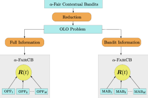
Figure 1: Diagram representing the web of reductions used in the paper. First, the contextual bandit problem with a global $\alpha$-fair objective is reduced to a standard online linear optimization (OLO) problem. The reduction works the same way in both the full-information and bandit-information feedback settings. Then, in either setting, we parallelly run $M$ instances of a non-contextual policy, and all the $M$ policies are coupled through the shared vector $\bm{R}(t)$ of cumulative rewards. On a high level, after the linearization step, the $j^{\text{th}}$ policy for $j\in[M]$ controls the regret for the $j$th context.

2.1 Algorithm design I: Linearization

Similar to Sinha et al. (2023), the algorithm design proceeds in two steps - (1) linearization with policy-dependent gradients and then (2) solving the linearized online optimization problem. See Figure 1 for a schematic. In the linearization step, we first reduce the problem to an instance of an online linear optimization (OLO) problem. Since the utility function $\phi(\cdot)$ is concave, we have

$$\phi(x)-\phi(y)\leq\phi^{\prime}(y)(x-y)$$ (4)

for all $x,y>0$. Now, let $\beta\geq 1$ be a constant, which will be fixed later. Taking $x=R_{i}^{*}(T)$ and $y=\beta R_{i}(T)$ in the above inequality, we get

$$\phi(R_{i}^{*}(T))-\beta^{1-\alpha}\phi(R_{i}(T))$$

$$\overset{(a)}{=}\phi(R_{i}^{*}(T))-\phi(\beta R_{i}(T))$$

$$\overset{(b)}{\leq}\phi^{\prime}(\beta R_{i}(T))[R_{i}^{*}(T)-\beta R_{i}(T)]$$

$$\overset{(c)}{\leq}\beta^{-\alpha}\phi^{\prime}(R_{i}(T))\sum_{t=1}^{T}r_{i}(t)[x^{c_{t}}_{*,i}-\beta x^{c_{t}}_{i}(t)],$$ (5)

where in $(a)$, we have used the property that $\phi(\beta x)=\beta^{1-\alpha}(x)$ which holds for (2); in $(b)$, we have used inequality (4), and in $(c)$, we have used the definition of the cumulative rewards given in (1), the fact that $\beta\geq 1$ and the property $\phi^{\prime}(\beta x)=\beta^{-\alpha}\phi^{\prime}(x)$. Summing up the bound (5) over all the arms $i\in[N]$, we obtain the following bound to the $\beta^{1-\alpha}$-approximate regret of any online policy:

$$\text{Regret}_{T}(\beta^{1-\alpha})$$

$$\leq\beta^{-\alpha}\sum_{t=1}^{T}\sum_{i\in[N]}\phi^{\prime}(R_{i}(T))r_{i}(t)[x^{c_{t}}_{*,i}-\beta x^{c_{t}}_{i}(t)].$$ (6)

Note that $R_{i}(T)$ is the cumulative reward accrued in the entire horizon of length $T$, and hence, it depends on the entire sequence of rewards and the actions of the policy. Clearly, this non-causal information is not available to the online policy at any intermediate round $t<T.$ This shows that directly minimizing the upper bound (2.1) using online convex optimization methods is not feasible as the reward function involves the variables $\phi^{\prime}(R_{i}(T))$’s. To get around this fundamental difficulty, we now define a surrogate online linear optimization problem by replacing the $t$^th coefficient $\phi^{\prime}(R_{i}(T))$ in the RHS of the upper bound (2.1) with its causal surrogate $\phi^{\prime}(R_{i}(t-1))$. With this substitution, the problem of minimizing (2.1) becomes an instance of the online linear optimization (OLO) problem. However, in contrast with the standard OLO problem, here the reward functions are no longer oblivious as they depend on the policy through its past actions. By bounding the regret of the surrogate problem, we show that it is possible to derive an approximate regret bound to the original regret minimization problem (3). Hence, dropping the factor $\beta^{-\alpha}$, the surrogate regret that we minimize is:

$$\text{Surrogate Regret}_{T}$$

$$=\max_{\bm{x}_{*}}\sum_{t=1}^{T}\sum_{i\in[N]}\phi^{\prime}(R_{i}(t-1))r_{i}(t)[x^{c_{t}}_{*,i}-x^{c_{t}}_{i}(t)]$$ (7)

In particular, for the surrogate problem, the linear reward vector at time step $t$ is given by $\phi^{\prime}(\bm{R}(t-1))\odot\bm{r}(t),$ which implicitly depends on the past actions of the policy (through the first term). Here, $\phi^{\prime}(\bm{R}(t-1))\equiv(\phi^{\prime}(R_{1}(t-1)),...,\phi^{\prime}(R_{N}(t-1)))$. Upon setting $\beta\equiv(1-\alpha)^{-1},$ the following result relates the original regret (3) with the surrogate regret (7) for any policy.

Lemma 2.1.

For any $T\geq 1$ and for any policy, we have

$$\emph{Regret}_{T}(c_{\alpha})\leq(1-\alpha)^{\alpha}\emph{Surrogate Regret}_{T}+c_{\alpha}N$$ (8)

where $c_{\alpha}=(1-\alpha)^{-(1-\alpha)}\leq e^{1/e}<1.445$.

After accounting for $M$ different contexts with a common cumulative reward vector $\bm{R}(t)$, the proof generalizes the arguments in Sinha et al. (2023, Lemma 1). See Section 6.1 in the Appendix for the complete proof.

2.2 Algorithm design II: Solving the linearized problem with full information

In view of the regret bound (8), we now propose $\alpha\textsc{-FairCB}$ - an online policy to approximately minimize the surrogate regret (7). In brief, $\alpha\textsc{-FairCB}$ runs $M$ instances of adaptive online gradient descent policy in parallel, where the $j$^th instance is responsible for controlling the regret for the $j$^th context. These parallel policies are coupled through the common state vector $\bm{R}(t)$ - the cumulative reward accrued up to time $t$, which is affected by all contexts. Technically, this strategy works because, after the linearization step above, using the Cauchy-Scwarz inequality, the regret can be upper-bounded by the sum of policy-dependent gradients over all $M$ instances. Finally, the norm of these policy-dependent gradients are controlled using a novel bootstrapping technique. The following lemma gives a precise regret bound for the surrogate problem.

Lemma 2.2.

The $\alpha\textsc{-FairCB}$ policy described in Algorithm 1 achieves the following static regret bound for the surrogate problem (7):

$$\emph{Surrogate Regret}_{T}=\begin{cases}O(N^{3}MT^{1/2-\alpha}),&\text{if }0<\alpha<\frac{1}{2}\\ O(N^{3}M\sqrt{\log T}),&\text{if }\alpha=\frac{1}{2}\\ O(1),&\text{if }\frac{1}{2}<\alpha<1.\end{cases}$$ (9)

See Section 6.2 for the proof of the result. The proof of this lemma exploits a novel bootstrapping technique which repeatedly boosts the estimate of the gradients, which are controlled by the policy, to obtain a better adaptive regret bound. Combining Lemma 2.1 and Lemma (2.2), we establish our main result.

Theorem 2.3.

Algorithm 1 achieves the following approximate regret bound for the contextual bandit problem in the full information setting with the $\alpha$-fair utility function:

$$\emph{Regret}_{T}(c_{\alpha})=(1-\alpha)^{\alpha}\begin{cases}O(N^{3}MT^{1/2-\alpha}),\text{if }0<\alpha<\frac{1}{2}\\ O(N^{3}M\sqrt{\log T}),\text{if }\alpha=\frac{1}{2}\\ O(1),~{}\text{if }\frac{1}{2}<\alpha<1.\end{cases}$$

where $c_{\alpha}=(1-\alpha)^{-(1-\alpha)}<1.445$.

Algorithm 1 $\alpha\textsc{-FairCB}$ (Full Information Setting)

1:Input: Fairness parameter $0\leq\alpha<1$, Sequence of reward vectors $\bm{r}(1)$, …, $\bm{r}(T)$, Sequence of contexts $c_{1},...,c_{T}$, Euclidean projection oracle on the simplex $\Pi_{\Delta_{N}}$, and an upper bound $D=\sqrt{2}$ to the Euclidean diameter of the simplex $\Delta_{N}$.

2:Output: Distributions $\bm{x}^{c_{t}}(t)$ for each round $t$.

3:Initialization:

$$R_{i}(0)\leftarrow 1,S_{j}\leftarrow 0,\bm{x}^{j}\leftarrow\dfrac{\bm{1}}{N},~{}\forall i,j.$$

4:for $t=1$ to $T$ do

5:   Receive the context $c_{t}$ for round $t$.

6:   if Context $c_{t}$ is seen for the first time then

7:      Output $\bm{x}^{c_{t}}(t)=\bm{x}^{c_{t}}$ (uniform distribution).

8:   else

9:      Let $t^{\prime}$ be the last time step when context $c_{t}$ was seen.

10:      Compute gradient vector $\bm{g}$ as follows:

$$g_{i}=\dfrac{r_{i}(t^{\prime})}{R_{i}^{\alpha}}\quad\forall i\in[N]$$

11:      Update the cumulative gradient norm:

$$S_{c_{t}}\leftarrow S_{c_{t}}+\lVert\bm{g}\rVert_{2}^{2}$$

12:      Carry out the online gradient ascent update:

$$\bm{x}^{c_{t}}\leftarrow\Pi_{\Delta_{N}}\left(\bm{x}^{c_{t}}+\dfrac{D}{\sqrt{2S_{c_{t}}}}\bm{g}\right)$$

13:      Output $\bm{x}^{c_{t}}(t)=\bm{x}^{c_{t}}$.

14:   end if

15:   Observe reward vector $\bm{r}(t)$.

16:   Update $R_{i}(t)\leftarrow R_{i}(t-1)+x^{c_{t}}_{i}(t)r_{i}(t)$.

17:end for

3 The Bandit feedback setting

We now study the same problem in the more challenging bandit feedback model. In this setup, only the reward of the arm selected by the policy, i.e., $r_{I_{t}}^{c_{t}}(t)$, is revealed on each round. Following standard practice, we assume that the reward vectors $\bm{r}(t)$ and the context sequence $c_{t}\in[M]$ for each time step $t$ are generated by an oblivious adversary, i.e., the sequence of rewards and contexts is fixed a priori.

Because of the limited feedback, an online policy cannot observe the expected cumulative rewards defined in Eqn. (1) as one needs to know the entire reward vector $\bm{r}(t)$ to compute the expected reward. Hence, instead of using the distribution $\bm{x}^{c_{t}}(t)$, we directly use the random one-hot encoded vector $\bm{X}^{c_{t}}(t)$ to define the true cumulative rewards . Here, the $I_{t}$ ^th component (which corresponds to the selected arm) of the vector $\bm{X}^{c_{t}}(t)$ is set to one, and the rest of the components are set to zero. Hence, the true cumulative reward vector, which the policy can observe under the bandit feedback setting, evolves as follows:

$$R_{i}(t) =R_{i}(t-1)+X^{c_{t}}_{i}(t)r_{i}(t),~{}R_{i}(0)=1.$$ (10)

As before, we will use the notation $\bm{x}^{c_{t}}(t)\in\Delta_{N}$ to denote the probability distribution of pulling the arms on step $t$. Hence, for all $i\in[N]$ and $t\in[1,T]$, we have

$$\mathbb{P}[X^{c_{t}}_{i}(t)=1]=x^{c_{t}}_{i}(t).$$ (11)

Our objective is to design a policy which minimizes the expected $c$-approximate regret defined below:

$$\text{Regret}_{T}(c)$$

$$:=\max_{\bm{x}_{*}\in(\Delta_{N})^{M}}\mathbb{E}\left[\sum_{i\in[N]}\phi(R_{i}^{*}(T))-c\sum_{i\in[N]}\phi(R_{i}(T))\right].$$ (12)

In the above definition, $c\geq 1$ is a small constant whose value will be specified later and $\bm{R}^{*}(T)$ is the cumulative reward vector obtained for a stationary contextual bandit policy which pulls arms according to the fixed collection of distributions $\bm{x}_{*}\equiv(\bm{x}^{1}_{*},...,\bm{x}^{M}_{*})$ depending on the current context. Let $(\bm{x}^{1}_{*},...,\bm{x}^{M}_{*})\in(\Delta_{N})^{M}$ be the best-fixed collection of distributions which achieves the maximum in (12). We have

$$\text{Regret}_{T}(c)$$

$$=\mathbb{E}\left[\sum_{i\in[N]}\phi(R_{i}^{*}(T))-c\sum_{i\in[N]}\phi(R_{i}(T))\right]$$

$$\overset{(a)}{=}\sum_{i\in[N]}\mathbb{E}[\phi(R_{i}^{*}(T))]-c\mathbb{E}\left[\sum_{i\in[N]}\phi(R_{i}(T))\right]$$

$$\overset{(b)}{\leq}\sum_{i\in[N]}\phi(\mathbb{E}[R_{i}^{*}(T)])-c\mathbb{E}\left[\sum_{i\in[N]}\phi(R_{i}(T))\right]$$

$$\overset{(c)}{=}\sum_{i\in[N]}\phi\left(1+\sum_{t=1}^{T}r_{i}(t)x^{c_{t}}_{*,i}\right)-c\mathbb{E}\left[\sum_{i\in[N]}\phi(R_{i}(T))\right]$$ (13)

Above, in $(a)$, we have used the linearity of expectation. In $(b)$, we have used Jensen’s Inequality on the concave function $\phi$. In $(c)$, we have just expanded $\mathbb{E}[R_{i}^{*}(T)]$ using (10) and (11).

3.1 Algorithm design I: Linearization

Similar to the full-information setting, we handle the non-linearity by reducing the problem to a standard bandit problem with appropriately constructed linear reward functions. Following (5), we have

$$\phi(\mathbb{E}R_{i}^{*}(T))-\beta^{1-\alpha}\phi(R_{i}(T))$$

$$\leq\beta^{-\alpha}\phi^{\prime}(R_{i}(T))\sum_{t=1}^{T}r_{i}(t)[x^{c_{t}}_{*,i}-\beta X^{c_{t}}_{i}(t)]$$ (14)

where above, $\beta\geq 1$ is some constant to be fixed later. Summing the above inequality for all $i\in[N]$ and taking expectations w.r.t the actions of the policy, we have

$$\sum_{i\in[N]}\phi(\mathbb{E}R_{i}^{*}(T))-\beta^{1-\alpha}\mathbb{E}\left[\sum_{i\in[N]}\phi(R_{i}(T))\right]$$

$$\leq\beta^{-\alpha}\mathbb{E}\left[\sum_{i\in[N]}\sum_{t=1}^{T}\phi^{\prime}(R_{i}(T))r_{i}(t)[x^{c_{t}}_{*,i}-\beta X^{c_{t}}_{i}(t)]\right].$$ (15)

Combining the last inequality with (3), we get

$$\text{Regret}_{T}(\beta^{1-\alpha})$$

$$\leq\beta^{-\alpha}\mathbb{E}\left[\sum_{i\in[N]}\sum_{t=1}^{T}\phi^{\prime}(R_{i}(T))r_{i}(t)[x^{c_{t}}_{*,i}-\beta X^{c_{t}}_{i}(t)]\right].$$ (16)

Motivated by the above bound, we now consider a surrogate bandit problem by replacing the term $\phi^{\prime}(R_{i}(T))$ with its causal counterpart $\phi^{\prime}(R_{i}(t-1))$. We now design an online policy to minimize the surrogate regret defined as follows:

$$\text{Surrogate Regret}_{T}$$

$$\equiv\mathbb{E}\left[\sum_{i\in[N]}\sum_{t=1}^{T}\phi^{\prime}(R_{i}(t-1))r_{i}(t)[x^{c_{t}}_{*,i}-X^{c_{t}}_{i}(t)]\right]$$

$$=\mathbb{E}\left[\sum_{t=1}^{T}\langle\phi^{\prime}(\bm{R}(t-1))\odot\bm{r}(t),\bm{x}^{c_{t}}_{*}-\bm{X}^{c_{t}}(t)\rangle\right].$$ (17)

As before, $\phi^{\prime}(\bm{R}(t-1))\equiv(\phi^{\prime}(R_{1}(t-1)),...,\phi^{\prime}(R_{N}(t-1)))$. Analogous to Lemma 2.1, we have the following result, which relates the regret defined in (12) to the surrogate regret defined in (17).

Lemma 3.1.

For any $T\geq 1$, we have

$$\emph{Regret}_{T}(c_{\alpha})\leq(1-\alpha)^{\alpha}\emph{Surrogate Regret}_{T}+c_{\alpha}N,$$ (18)

where $c_{\alpha}=(1-\alpha)^{-(1-\alpha)}\leq e^{1/e}<1.445$.

3.2 Algorithm design II: Solving the linearized problem with bandit feedback

Lemma 3.1 motivates us to design an online policy that minimizes the regret (17) for the surrogate bandit problem. However, unlike the standard adversarial bandit problem, where the reward functions are fixed a priori in an oblivious fashion, in this case, the rewards for each round $t$, defined as $\bm{g}_{t}\equiv\phi^{\prime}(\bm{R}(t-1))\odot\bm{r}_{t},$ depends on the past actions of the policy. We can decompose the surrogate regret over the contexts as follows:

$$\mathbb{E}\left[\sum_{t=1}^{T}\langle\bm{g}_{t},\bm{x}^{c_{t}}_{*}-\bm{X}^{c_{t}}(t)\rangle\right]$$

$$=\mathbb{E}\left[\sum_{j\in[M]}\sum_{t:c_{t}=j}\langle\bm{g}_{t},\bm{x}^{j}_{*}-\bm{X}^{j}(t)\rangle\right]$$

$$\overset{(a)}{=}\sum_{j\in[M]}\mathbb{E}\left[\sum_{t:c_{t}=j}\langle\bm{g}_{t},\bm{x}^{j}_{*}-\bm{X}^{j}(t)\rangle\right]$$

$$\overset{(b)}{\leq}\sum_{j\in[M]}\underbrace{\mathbb{E}\left[\max_{y\in\{\bm{e}_{k}\}_{k=1}^{N}}\sum_{t:c_{t}=j}\langle\bm{g}_{t},\bm{y}-\bm{X}^{j}(t)\rangle\right]}_{\textrm{regret for the}~{}j\textsuperscript{th}~{}\textrm{context}}$$

$$=:\hat{\text{Regret}}_{T}.$$ (19)

Above, in $(a)$, we have used the linearity of expectation, in $(b)$, we have used the fact that for any fixed sequence of rewards in a bandit OLO problem, the best offline benchmark is the best-fixed arm in hindsight. The above inequality can be written as

$$\text{Surrogate Regret}_{T}\leq\hat{\text{Regret}}_{T}$$ (20)

To minimize the surrogate regret, we now design a policy that minimizes $\hat{\text{Regret}}_{T}$, which is the sum of the regret for each context. Note that since the cumulative reward vector is common to all contexts, the regret bounds for different contexts are coupled with each other. To solve the per-context learning problem, we use the adaptive and scale-free multi-armed bandit policy, proposed by (Putta and Agrawal, 2022), as a black box. Specifically, we run $M$ parallel instances of this policy, one for each context where they share the global cumulative reward vector $\bm{R}(t).$ For ease of reference, we quote regret bound achieved by the bandit policy of Putta and Agrawal (2022) in the following theorem.

Algorithm 2 $\alpha\textsc{-FairCB}$ (Bandit Information Setting)

1:Input: Fairness parameter $0\leq\alpha<1$, Sequence of reward vectors $\bm{r}(1)$, …, $\bm{r}(T)$, Sequence of contexts $c_{1},...,c_{t}$.

2:Output: Arm $I_{t}\in[N]$ to be played at round $t$, for $t\in[1,T]$.

3:Initialize $R_{i}(0)\leftarrow 1$ for all $i\in[N]$.

4:Initialize $M$ adaptive, scale-free MAB policies from Putta and Agrawal (2022). Let $\mathscr{A}_{j}$ denote the $j$th instance of the policy, for $j\in[M]$.

5:for $t=1$ to $T$ do

6:   Observe context $c_{t}$.

7:   Play an arm $I_{t}$ picked by policy $\mathscr{A}_{c_{t}}$. Let $\bm{X}^{c_{t}}(t)$ denote the one-hot vector representing arm $I_{t}$.

8:   Feed the modified reward vector $\phi^{\prime}(\bm{R}(t-1))\odot\bm{r}(t)$ to policy $\mathscr{A}_{c_{t}}$.

9:   Update $R_{i}(t)\leftarrow R_{i}(t-1)+X^{c_{t}}_{i}(t)r_{i}(t)$ for all $i\in[N]$.

10:end for

Theorem 3.2 (Theorem 1 of (Putta and Agrawal, 2022)).

For any oblivious sequence of reward vectors $\bm{l}_{1},...,\bm{l}_{T}\in\mathbb{R}^{N}$, the adaptive version of Algorithm 1 of Putta and Agrawal (2022) achieves the following regret bound:

$$\mathbb{E}\left[\max_{\{\bm{e}_{k}\}_{k=1}^{N}}\sum_{t=1}^{T}\langle\bm{l}_{t},\bm{e}_{k}-\bm{X}(t)\rangle\right]$$

$$=O(\log T\cdot[\sqrt{NL_{2}}+L_{\infty}\sqrt{NL_{1}}]).$$ (21)

In the above, $\bm{X}(t)$ is the one-hot encoded vector denoting the arm pulled on round $t$, $L_{\infty}=\max_{t}\lVert\bm{l}_{t}\rVert_{\infty}$, $L_{2}=\sum_{t=1}^{T}\lVert\bm{l}_{t}\rVert_{2}^{2}$, $L_{1}=\sum_{t=1}^{T}\lVert\bm{l}_{t}\rVert_{1}$ and the expectation is taken w.r.t. the actions of the policy.

Remarks:

Technically, the regret bound in Theorem 3.2 was originally established for oblivious adversaries. However, in our case, the surrogate reward vector $\bm{g}_{t}$ depends on the past actions of the policy up to round $t-1$. To see why we can still plug in the generic regret bound (3.2), note that the reward vector $\bm{g}_{t}$ on round $t$ does not depend on the action $\bm{X}(t)$ taken on round $t$. Hence, we can use the regret bound for an imaginary adversary that fixes the reward vector $\bm{g}_{t}$ at the end of round $t-1$. Since the reward on round $t$ does not affect the previous actions of the policy, the regret bound (3.2) holds. Adapting the above bound to our contextual setting, we have the following scale-free regret bound.

Lemma 3.3.

For any $t\in[1,T]$, let $\bm{g}_{t}:=\phi^{\prime}(\bm{R}(t-1))\odot\bm{r}(t)$. The adaptive version of Algorithm 1 of (Putta and Agrawal, 2022) achieves the following bound for any $j\in[M]$:

$$\mathbb{E}\left[\max_{y\in\{\bm{e}_{k}\}_{k=1}^{N}}\sum_{t:c_{t}=j}\langle\bm{g}_{t},\bm{y}-\bm{X}^{j}(t)\rangle\right]\leq$$

$$\tilde{O}\left(\mathbb{E}\left[\sqrt{N\sum_{t:c_{t}=j}\lVert\bm{g}_{t}\rVert_{2}^{2}}+\max_{t:c_{t}=j}\lVert\bm{g}_{t}\rVert_{\infty}\sqrt{N\sum_{t:c_{t}=j}\lVert\bm{g}_{t}\rVert_{1}}\right]\right),$$ (22)

where the $\tilde{O}(\cdot)$ notation hides the logarithmic factors. Above, the expectation is taken w.r.t the policy actions.

Please refer to Section 6.5 for the proof. The following result bounds the surrogate regret (19).

Lemma 3.4.

The $\alpha\textsc{-FairCB}$ policy described in Algorithm 2 achieves the following bound on the regret of the surrogate bandit OLO problem for the $\alpha$-fair utility function:

$$\hat{\emph{Regret}}_{T}=\tilde{O}(MN^{2}T^{\frac{1-\alpha}{2}})$$ (23)

where the $\tilde{O}(\cdot)$ notation hides the $\log T$ factor.

Finally, combining Lemma 3.1, (20) and Lemma 3.4, we establish our main result.

Theorem 3.5.

Algorithm 2 achieves the following approximate regret bound for the contextual bandit problem in the bandit information feedback setting with the $\alpha$-fair utility function:

$$\emph{Regret}_{T}(c_{\alpha})=(1-\alpha)^{\alpha}\tilde{O}(MN^{2}T^{\frac{1-\alpha}{2}})$$ (24)

where $c_{\alpha}=(1-\alpha)^{-(1-\alpha)}<1.445$, and the $\tilde{O}$ notation hides factors logarithmic in $T$.

4 Experiments

We evaluate the performance of the proposed algorithm on a movie genre recommendation problem using the MovieLens 25M dataset (Harper and Konstan, 2015). The dataset consists of 25 million data points, each consisting of a movie rating given by a user. For our experiments, we take a small sample comprising of the first $5,000$ data points. The underlying contextual bandit problem is formulated as follows: we interpret the users as contexts and movie genres as arms. In the selected sample, the number of contexts turns out to be $M=33$, and the number of arms featured is $N=19$. The dataset is sorted by the column containing the timestamps at which the ratings were reported, and this is taken to be the order of request arrivals. Since our policy requires a positive lower bound to the rewards, we take the minimum reward to be $0.2$ if the recommended genre doesn’t fit the current movie and $1$ otherwise. In our experiments, we study both the full information and the bandit information settings.

Performance metrics: We define the $\alpha$-performance of a policy at time stamp $t\in[1,T]$ in these experiments as the total $\alpha$-fair utility:

$$\text{$\alpha$-Performance}(t):=\sum_{i\in[N]}\phi(R_{i}(t)).$$ (25)

To measure fairness, we use the popular Jain’s Fairness Index (Jain et al., 1998), calculated for the vector of cumulative rewards at the end of the time horizon. For any round $t\in[1,T]$, Jain’s fairness index is defined as:

$$\text{Jain's Fairness Index}:=\dfrac{(\sum_{i=1}^{N}R_{i}(t))^{2}}{N\sum_{i=1}^{N}R_{i}^{2}(t)}.$$ (26)

Jain’s fairness index assumes a value between $0$ and $1$, where a value of $1$ is obtained when all components of the reward vector are the same (i.e., fully fair). In particular, if each arm receives an equal share of cumulative rewards, this index will be $1$. Throughout our experiments, we take $\alpha=0.9$ (i.e. a high level of fairness). We also plot the approximate contextual regret as defined in equations (3) and (12) for the full information and bandit feedback settings, respectively.

Calculating the offline baseline metrics: Note that the offline benchmarks in equations (3) and (12) required for computing the approximate regret involve computing the best offline collection of $M$ distributions maximizing the cumulative $\alpha$-fair utility function. Since $\phi(\cdot)$ is a concave function, this is a standard concave maximization problem over the convex domain $(\Delta_{N})^{M}$. In our experiments, we use the CVXPY package for solving this problem (Diamond and Boyd, 2016).

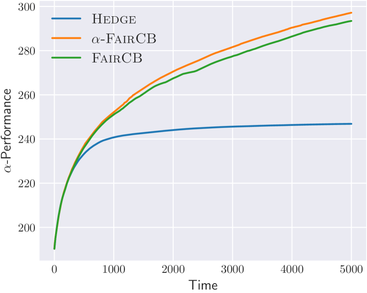
Figure 2: $\alpha$-performance for the full information setting.

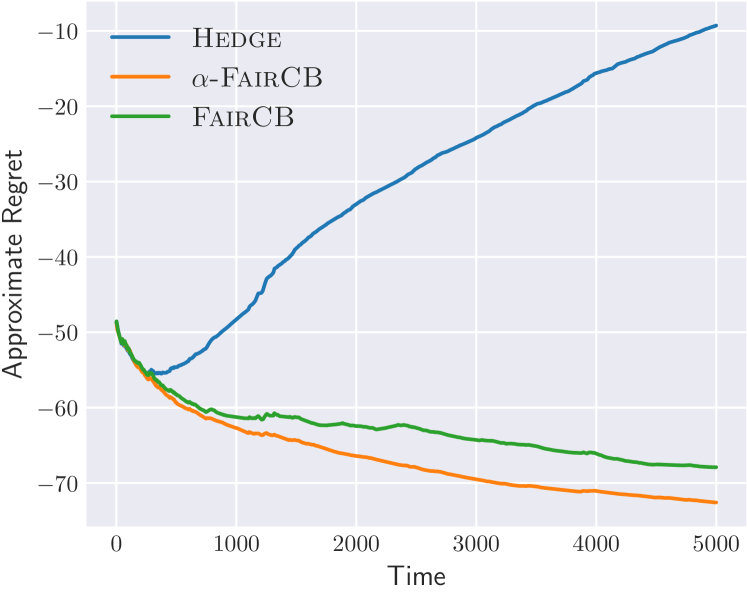
Figure 3: Approximate regret for the full information setting.

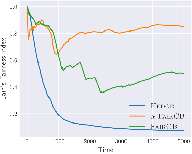
Figure 4: Jain’s Fairness Index for the full information setting.

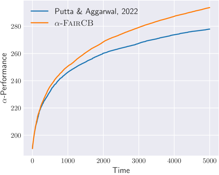
Figure 5: $\alpha$-performance for the bandit information setting.

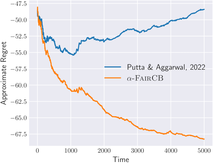
Figure 6: Approximate regret for the bandit information setting.

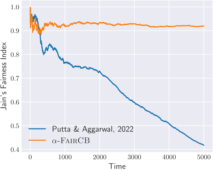
Figure 7: Jain’s Fairness Index for the bandit information setting.

4.1 Experiments in the Full-information Setting

Baseline Policies: We consider two baselines (1) a context-agnostic Hedge policy (i.e. a policy that ignores contexts) and (2) the FairCB policy from (Chen et al., 2020). Note that inherently Hedge is not a fair policy as its objective is to optimize the total reward. On the other hand, FairCB’s fairness constraint is specified by a tunable parameter $\nu\in(0,\frac{1}{N})$; in particular, the constraint is that the marginal probability of each arm being pulled at any given time step is at least $\nu$. For our experiments, we consider $\nu=\frac{1}{2N}$ (note that $\frac{1}{N}$ is the largest possible fairness level that is allowed by FairCB). Note that the FairCB policy assumes the context distribution to be known; we simply generate this distribution offline by observing the sequence of contexts (users) in the dataset (and generating a distribution based on the frequencies of each user) and feed it back to the FairCB policy.

Results: Figure 4 shows that the proposed $\alpha\textsc{-FairCB}$ policy outperforms the Hedge and FairCB policies in terms of $\alpha$-performance (25). As expected, the context-agnostic Hedge policy performs the worst among the three policies under consideration. Consequently, $\alpha\textsc{-FairCB}$ achieves the lowest approximate regret among all the policies (Figure 4). Finally, in terms of Jain’s Fairness Index (26), we observe that the proposed $\alpha\textsc{-FairCB}$ outperforms both the non-contextual Hedge and FairCB policies even for a moderately large time horizon (Figure 4).

4.2 Experiments in the Bandit Setting

Baseline Policies: As a baseline policy, we run the context-agnostic adaptive multi-armed bandit policy proposed by Putta and Agrawal (2022), which is also used by our contextual bandit policy as a subroutine.

Results: From Figure 7, it is observed that $\alpha\textsc{-FairCB}$ outperforms the policy by (Putta and Agrawal, 2022) in terms of $\alpha$-performance, and consequently $\alpha\textsc{-FairCB}$ achieves a lower approximate regret as well (as seen in Figure 7). In terms of Jain’s Fairness Index, it is observed from Figure 7 that although for the first few rounds, (Putta and Agrawal, 2022)’s policy outperforms $\alpha\textsc{-FairCB}$, but over the entire time horizon, $\alpha\textsc{-FairCB}$ achieves a significantly better fairness index. The behaviour for the first few time steps can be explained by the fact that Putta and Agrawal (2022)’s policy has an exploration component, which makes the policy choose each arm with an approximately equal probability in the initial stages. However, since their policy maximizes the cumulative rewards, it achieves a worse fairness index over a longer horizon. See Section 7 in the Appendix for additional experimental results.

5 Conclusion and Future Work

In this paper, we considered the problem of learning adversarial unstructured context-to-reward mapping and proposed an approximately regret-optimal policy in the full-information and bandit feedback setting. In the future, it will be interesting to design efficient algorithms for the case of structured contexts. Finally, similar to Chen et al. (2020), designing $\alpha$-fair bandit algorithms that guarantee a fixed fraction of pulls to each arm would also be interesting to investigate.

6 Appendix

6.1 Proof of Lemma 2.1

Before proving the claim, we establish an auxiliary result that will be useful later.

Lemma 6.1.

Under any policy which updates the cumulative rewards of the $i$^th user $R_{i}(\cdot)$ as in (1) $\forall i\in[N]$, the following inequality holds:

$$\phi^{\prime}(R_{i}(t-1))[R_{i}(t)-R_{i}(t-1)]\leq\int_{R_{i}(t-1)-1}^{R_{i}(t)-1}\phi^{\prime}(R)\emph{d}R.$$ (27)

Proof.

Since $0\leq\alpha<1$, observe that the utility function $\phi(\cdot)$ given by Eq.  (2) is well-defined on $[0,\infty)$ and is differentiable in $(0,\infty)$. Also, because $R_{i}(\cdot)$ is monotonically non-decreasing and $R_{i}(0)=1$, we note that $R_{i}(t-1)-1\geq 0$ for all $t\in[1,T]$. By the fundamental theorem of calculus combined with the mean value theorem, we have

$$\int_{R_{i}(t-1)-1}^{R_{i}(t)-1}\phi^{\prime}(R)\text{d}R=\phi^{\prime}(c_{0})[R_{i}(t)-R_{i}(t-1)]$$ (28)

for some $c_{0}\in(R_{i}(t-1)-1,R_{i}(t)-1)$; in particular, we have $c_{0}<R_{i}(t)-1$. Now, from the defintion (1) observe that $R_{i}(t)-R_{i}(t-1)=x^{c_{t}}_{i}(t)r_{i}(t)\leq 1$, where we have used the fact that $x^{c_{t}}_{i}(t),r_{i}(t)\leq 1$. This implies that $R_{i}(t)-1\leq R_{i}(t-1)$, and hence, $c_{0}<R_{i}(t-1)$.

Finally, since $\phi(\cdot)$ is concave, $\phi^{\prime}(\cdot)$ is non-increasing; this implies that $\phi^{\prime}(c_{0})\geq\phi^{\prime}(R_{i}(t-1))$. Combining this with (28), the claim follows. ∎

We now establish Lemma 2.1.

Proof.

The upper bound for $\text{Regret}_{T}(\beta^{1-\alpha})$ from Eq. (2.1) can be split into the difference of two terms $A$ and $B$ as defined below:

$$\text{Regret}_{T}(\beta^{1-\alpha})\leq\beta^{-\alpha}[A-\beta B],$$ (29)

where

$$A =\sum_{i\in[N]}\phi^{\prime}(R_{i}(T))\sum_{t=1}^{T}r_{i}(t)x^{c_{t}}_{*,i},$$ (30)

$$B =\sum_{i\in[N]}\phi^{\prime}(R_{i}(T))\sum_{t=1}^{T}r_{i}(t)x^{c_{t}}_{i}(t).$$ (31)

Also, let $A^{\prime}$ and $B^{\prime}$ denote the corresponding terms in the regret expression (7) for the surrogate OLO problem. We will now bound the terms $A$ and $B$ in terms of $A^{\prime}$ and $B^{\prime}$, respectively.

Proving $A\leq A^{\prime}$: Note that the utility function $\phi(\cdot)$ is concave, and hence its derivative is non-increasing. Also, from the recurrence equation for the cumulative rewards (1), it is clear that under any policy, $R_{i}(\cdot)$ is non-decreasing for any $i\in[N]$. Hence, we see that $\phi^{\prime}(R_{i}(t-1))\geq\phi^{\prime}(R_{i}(T))$ for all $t\in[1,T]$ and $i\in[N]$. This implies that

$$A =\sum_{i\in[N]}\phi^{\prime}(R_{i}(T))\sum_{t=1}^{T}r_{i}(t)x^{c_{t}}_{*,i}$$

$$\leq\sum_{i\in[N]}\phi^{\prime}(R_{i}(t-1))\sum_{t=1}^{T}r_{i}(t)x^{c_{t}}_{*,i}$$

$$=A^{\prime}$$ (32)

Proving $B^{\prime}\leq(1-\alpha)^{-1}(B+N)$: We now argue that the following set of inequalities holds:

$$B^{\prime} =\sum_{i}\sum_{t=1}^{T}\phi^{\prime}(R_{i}(t-1))r_{i}(t)x^{c_{t}}_{i}(t)$$

$$\overset{(a)}{=}\sum_{i}\sum_{t=1}^{T}\phi^{\prime}(R_{i}(t-1))[R_{i}(t)-R_{i}(t-1)]]$$

$$\overset{(b)}{\leq}\sum_{i}\sum_{t=1}^{T}\int_{R_{i}(t-1)-1}^{R_{i}(t)-1}\phi^{\prime}(R)\text{d}R$$

$$\overset{(c)}{\leq}\sum_{i}\int_{0}^{R_{i}(T)}\phi^{\prime}(R)\text{d}R$$

$$\overset{(d)}{=}\sum_{i}\phi(R_{i}(T))$$

$$\overset{(e)}{=}(1-\alpha)^{-1}\sum_{i}\phi^{\prime}(R_{i}(T))R_{i}(T)$$

$$\overset{(f)}{=}(1-\alpha)^{-1}\sum_{i\in[N]}\phi^{\prime}(R_{i}(T))\left(1+\sum_{t=1}^{T}x^{c_{t}}_{i}(t)r_{i}(t)\right)$$

$$\overset{(h)}{\leq}(1-\alpha)^{-1}(B+N)$$ (33)

where in $(a),$ we have used the recurrence for $R_{i}(\cdot)$ as given in (1). In $(b)$, we have used (27). In $(c)$, we have simply used the fact that $R_{i}(0)-1=0$ and $R_{i}(T)-1\leq R_{i}(T)$. In $(d)$, we have used the fundamental theorem of calculus and the fact that $\phi(0)=0$. In $(e)$, we have used the fact that $x\phi^{\prime}(x)=(1-\alpha)\phi(x)$ which holds for the $\alpha$-fair utility function $\phi(\cdot)$. In $(f)$, we have used the definition of the cumulative rewards as in (1). In $(h)$, we have used the definition of $B$ and the fact that $\phi^{\prime}(x)=x^{-\alpha}\leq 1$ for all $x\geq 1$.

Now, the inequality $B^{\prime}\leq(1-\alpha)^{-1}(B+N)$ implies that $(1-\alpha)B^{\prime}-N\leq B$. Since $\beta>0$, we have $\beta B\geq\beta(1-\alpha)B^{\prime}-\beta N$. Combining this with $A\leq A^{\prime}$, we have that

$$A-\beta B\leq A^{\prime}-\beta(1-\alpha)B^{\prime}+\beta N.$$ (34)

Now, pick $\beta=(1-\alpha)^{-1}$ (which ensures that $\beta\geq 1$), and hence we obtain

$$A-\beta B\leq A^{\prime}-B^{\prime}+(1-\alpha)^{-1}N,$$ (35)

and from Eq. (29), we see that

$$\text{Regret}_{T}(c_{\alpha}) \leq(1-\alpha)^{\alpha}(A^{\prime}-B^{\prime})+c_{\alpha}N$$

$$=(1-\alpha)^{\alpha}\text{Surrogate Regret}_{T}+c_{\alpha}N,$$ (36)

which completes the proof of the lemma. ∎

6.2 Proof of Lemma 2.2

For ease of notation, let $(\bm{x}^{1}_{*},...,\bm{x}^{M}_{*})\in(\Delta_{N})^{M}$ be the collection of distributions achieving the maximum in equation (7). Now, observe that $\text{Surrogate Regret}_{T}$ defined in (7) for the surrogate problem can be split into the sum of regrets over each of the contexts as follows:

$$\text{Surrogate Regret}_{T} =\sum_{t=1}^{T}\langle\phi^{\prime}(\bm{R}(t-1))\odot\bm{r}(t),\bm{x}^{c_{t}}_{*}-\bm{x}^{c_{t}}(t)\rangle$$

$$=\sum_{j\in[M]}\sum_{t:c_{t}=j}\langle\phi^{\prime}(\bm{R}(t-1))\odot\bm{r}(t),\bm{x}^{j}_{*}-\bm{x}^{j}(t)\rangle$$

$$\overset{(a)}{\leq}\sum_{j\in[M]}\underbrace{\max_{\bm{x}^{j}_{\circ}\in\Delta_{N}}\sum_{t:c_{t}=j}\langle\phi^{\prime}(\bm{R}(t-1))\odot\bm{r}(t),\bm{x}^{j}_{\circ}-\bm{x}^{j}(t)\rangle}_{\text{Regret for the $j^{\text{th}}$ context}}$$ (37)

where above in $(a)$, we have simply used that the regret w.r.t $\bm{x}^{j}_{*}$ for context $j$ is upper bounded by the regret associated to the best offline benchmark $\bm{x}^{j}_{\circ}$ for context $j$.

Next, from the pseudocode of $\alpha\textsc{-FairCB}$ (Full Information Version, Algorithm 1), note that a Projected Online Gradient Ascent (OGA) policy with adaptive step sizes (Theorem 4.14 of (Orabona, 2019)) controls the regret for each context $j\in[M]$. For the sake of completeness, we mention the complete statement of the regret guarantee of the OGA policy.

Theorem 6.2 (Theorem 4.14 of (Orabona, 2019)).

Let $\Delta\subset\mathbb{R}^{d}$ be a convex set with diameter $D$. Let us consider a sequence of linear reward functions with gradients $\{\bm{g}_{t}\}_{t\geq 1}$. Run the Online Gradient Ascent policy with step sizes $\eta_{t}=\dfrac{D}{\sqrt{2}\sum_{\tau=1}^{T}\lVert\bm{g}_{\tau}\rVert^{2}}$, $1\leq t\leq T$. Then, the standard regret under the OGA policy can be upper bounded as follows:

$$\text{Regret}_{T}\leq D\sqrt{2\sum_{t=1}^{T}\lVert\bm{g}_{t}\rVert^{2}}.$$ (38)

Note that, for our case we have $D=\sqrt{2}$. So, by the regret bound of the OGA policy (38), for any $j\in[M]$ we have

$$\max_{\bm{x}^{j}_{\circ}\in\Delta_{N}}\sum_{t:c_{t}=j}\langle\phi^{\prime}(\bm{R}(t-1))\odot\bm{r}(t),\bm{x}^{j}_{\circ}-\bm{x}^{j}(t)\rangle$$

$$\leq D\sqrt{2\sum_{t:c_{t}=j}\lVert\phi^{\prime}(\bm{R}(t-1))\odot\bm{r}(t)\rVert_{2}^{2}}$$

$$\overset{(a)}{\leq}D\sqrt{2\sum_{t:c_{t}=j}\lVert\phi^{\prime}(\bm{R}(t-1))\rVert_{2}^{2}}$$

$$\overset{(b)}{=}D\sqrt{2\sum_{t:c_{t}=j}\sum_{i\in[N]}\dfrac{1}{R_{i}^{2\alpha}(t-1)}}$$ (39)

where above in $(a)$, we have used the fact that $\bm{r}(t)\leq\bm{1}$ for all $t$, and in $(b)$ we have used the fact that $\phi^{\prime}(x)=x^{-\alpha}$. Now, summing (39) over all the contexts $j\in[M]$ and combining this with (37), we see that

$$\text{Surrogate Regret}_{T} \leq\sum_{j\in[M]}D\sqrt{2\sum_{t:c_{t}=j}\sum_{i\in[N]}\dfrac{1}{R_{i}^{2\alpha}(t-1)}}$$

$$=M\sum_{j\in[M]}\dfrac{1}{M}D\sqrt{2\sum_{t:c_{t}=j}\sum_{i\in[N]}\dfrac{1}{R_{i}^{2\alpha}(t-1)}}$$

$$\overset{(a)}{\leq}DM\sqrt{\dfrac{2}{M}\sum_{j\in[M]}\sum_{t:c_{t}=j}\sum_{i\in[N]}\dfrac{1}{R_{i}^{2\alpha}(t-1)}}$$

$$=D\sqrt{M}\sqrt{2\sum_{t=1}^{T}\sum_{i\in[N]}\dfrac{1}{R_{i}^{2\alpha}(t-1)}},$$ (40)

where above in $(a)$, we have used Jensen’s Inequality for the square root function. Using the fact that $R_{i}(t-1)\geq 1$ for all $t$, bound (40) implies that

$$\text{Surrogate Regret}_{T}\leq O(\sqrt{MNT}).$$ (41)

In the following, we show that the above $O(\sqrt{T})$ regret bound can be substantially improved using a novel bootstrapping technique described below.

Bootstrapping:

Note that the adaptive regret bound depends on the sum of the norm of gradients of the reward vectors, which are controlled by the policy itself. This is in sharp contrast with the usual OCO setting where the policy does not explicitly control the gradients, and the final regret bound is given in terms of the sum of the norm of gradients as given in (38). The bootstrapping technique starts with a trivial upper bound on the gradient norms and then uses the regret bound itself to improve the upper bounds on the gradient norms. This, in turn, improves the regret bound through the adaptive regret bound (38). The process is repeated a few times to get the best possible bound.

We now apply the general bootstrapping method to our problem. Note that by the definition of $\text{Surrogate Regret}_{T}$ in (7), we have the following inequality for any fixed collection $(\bm{x}^{1}_{0},...,\bm{x}^{M}_{0})\in(\Delta_{N})^{M}$ of distributions:

$$\sum_{t=1}^{T}\langle\phi^{\prime}(\bm{R}(t-1))\odot\bm{r}(t),\bm{x}^{c_{t}}(t)\rangle$$

$$\geq\sum_{t=1}^{T}\langle\phi^{\prime}(\bm{R}(t-1))\odot\bm{r}(t),\bm{x}^{c_{t}}_{0}\rangle-\text{Surrogate Regret}_{T}.$$ (42)

Also, using the fact that $x^{c_{t}}_{i}(t)r_{i}(t)=R_{i}(t)-R_{i}(t-1)$ and following the same calculations up to step (d) of (6.1), we see that

$$\sum_{t=1}^{T}\langle\phi^{\prime}(\bm{R}(t-1))\odot\bm{r}(t),\bm{x}^{c_{t}}(t)\rangle\leq\sum_{i\in[N]}\phi(R_{i}(T)).$$ (43)

Combining the above inequality with (6.2), we have

$$\sum_{i\in[N]}\phi(R_{i}(T))$$

$$\geq\sum_{t=1}^{T}\langle\phi^{\prime}(\bm{R}(t-1))\odot\bm{r}(t),\bm{x}^{c_{t}}_{0}\rangle-\text{Surrogate Regret}_{T}.$$ (44)

Next, we lower bound $\phi^{\prime}(\bm{R}(t-1))$ by $\phi^{\prime}(\bm{R}(T))$ and pick $\bm{x}^{j}_{0}=\frac{1}{N}\bm{1}$ for all $j\in[M]$ (i.e., we pick the uniform distribution as an offline benchmark for each context). Doing so, and using the fact that $\bm{r}(t)\geq\delta\bm{1}$ for all $t$, we have

$$\sum_{t=1}^{T}\langle\phi^{\prime}(\bm{R}(t-1))\odot\bm{r}(t),\bm{x}^{c_{t}}_{0}\rangle \geq\sum_{t=1}^{T}\langle\phi^{\prime}(\bm{R}(T))\odot\bm{r}(t),\bm{x}^{c_{t}}_{0}\rangle$$

$$=\sum_{i\in[N]}\sum_{t=1}^{T}\phi^{\prime}(R_{i}(T))r_{i}(t)\dfrac{1}{N}$$

$$\geq T\sum_{i\in[N]}\phi^{\prime}(R_{i}(T))\dfrac{\delta}{N}.$$ (45)

Plugging the last inequality in (44), we conclude that

$$\sum_{i\in[N]}\phi(R_{i}(T))\geq T\sum_{i\in[N]}\phi^{\prime}(R_{i}(T))\dfrac{\delta}{N}-\text{Surrogate Regret}_{T}.$$ (46)

Now, noting that $0<R_{i}(T)\leq T$ for all $i$, and that $\phi(\cdot)$ is monotone non-decreasing, we see that for any $i\in[N]$ the above inequality implies

$$\dfrac{NT^{1-\alpha}}{1-\alpha}\geq T\phi^{\prime}(R_{i}(T))\dfrac{\delta}{N}-\text{Surrogate Regret}_{T},$$ (47)

which implies the following inequality after dividing throughout by $T$ and replacing $\phi^{\prime}(R_{i}(T))$ by $\frac{1}{R_{i}^{\alpha}(T)}$:

$$\dfrac{N}{(1-\alpha)T^{\alpha}}\geq\dfrac{1}{R_{i}^{\alpha}(T)}\dfrac{\delta}{N}-\dfrac{\text{Surrogate Regret}_{T}}{T},$$ (48)

which is equivalent to

$$\dfrac{1}{R_{i}^{\alpha}(T)}\leq\dfrac{N}{\delta}\left[\dfrac{N}{(1-\alpha)T^{\alpha}}+\dfrac{\text{Surrogate Regret}_{T}}{T}\right].$$ (49)

Now, from Eq. (41), we have the following preliminary bound $\text{Surrogate Regret}_{T}\leq O(\sqrt{MNT})$. We use the bootstrapping technique by plugging this in (49) to derive the following improved bound on the cumulative reward accrued by the $i$^th arm.

$$\dfrac{1}{R_{i}^{\alpha}(T)}\leq O\left(\dfrac{N^{2}\sqrt{MN}}{T^{\min(1/2,\alpha)}}\right),~{}\forall i\in[N].$$ (50)

Now, we consider the following two cases:

Case 1: $0\leq\alpha\leq 1/2$. In this case, from (50) we see that $\frac{1}{R_{i}^{\alpha}(T)}\leq O(\frac{N^{2}\sqrt{MN}}{T^{\alpha}})$, and hence $\frac{1}{R_{i}^{2\alpha}(T)}\leq O(\frac{N^{5}M}{T^{2\alpha}})$. Note that this bound holds for all $T$. Hence, plugging this in (40), we get

$$\text{Surrogate Regret}_{T}\leq O\left(DN^{\frac{5}{2}}M\sqrt{2\sum_{t=2}^{T}\sum_{i\in[N]}\dfrac{1}{(t-1)^{2\alpha}}}\right)$$ (51)

If $0\leq\alpha<1/2$, the above bound becomes $\text{Surrogate Regret}_{T}\leq O\left(DN^{3}MT^{\frac{1}{2}-\alpha}\right)$. If $\alpha=\frac{1}{2}$, the above bound becomes $\text{Surrogate Regret}_{T}\leq O\left(DN^{3}M\sqrt{\log T}\right)$.

Case 2: $1/2<\alpha<1$. In this case, bound (50) implies that $\frac{1}{R_{i}^{\alpha}(T)}\leq\left(\dfrac{N^{2}\sqrt{MN}}{T^{1/2}}\right)$, and hence $\dfrac{1}{R_{i}^{2\alpha}(T)}\leq O\left(\dfrac{N^{5}M}{T}\right)$. Again, this is true for all $T$. So, plugging this in (40), we get

$$\text{Surrogate Regret}_{T} \leq O\left(DN^{\frac{5}{2}}M\sqrt{2\sum_{t=2}^{T}\sum_{i\in[N]}\dfrac{1}{(t-1)}}\right)$$

$$=O(DN^{3}M\sqrt{\log T})$$ (52)

Plugging this back in (49), we get that $\frac{1}{R_{i}^{\alpha}(T)}\leq O(\frac{N^{5}M}{T^{\alpha}})$, and hence $\frac{1}{R_{i}^{2\alpha}(T)}\leq O(\frac{N^{10}M^{2}}{T^{2\alpha}})$. Again, note that this holds for all $T$. Hence, plugging this in (40), we see that

$$\text{Surrogate Regret}_{T} \leq O\left(DN^{5}M^{\frac{3}{2}}\sqrt{2\sum_{t=2}^{T}\sum_{i\in[N]}\dfrac{1}{(t-1)^{2\alpha}}}\right)$$

$$=O(1)$$ (53)

where above, we have used the fact that $2\alpha>1$.

6.3 Proof of Lemma 3.1

The proof of Lemma 2.1 works here with minor modifications. Again, the upper bound in (16) for $\text{Regret}_{T}(\beta^{1-\alpha})$ can be split into the difference of two terms $A$ and $B$ as follows:

$$\text{Regret}_{T}(\beta^{1-\alpha})\leq\beta^{-\alpha}\mathbb{E}[A-\beta B]$$ (54)

where

$$A =\sum_{i\in[N]}\phi^{\prime}(R_{i}(T))\sum_{t=1}^{T}r_{i}(t)x^{c_{t}}_{*,i}$$ (55)

$$B =\sum_{i\in[N]}\phi^{\prime}(R_{i}(T))\sum_{t=1}^{T}r_{i}(t)X^{c_{t}}_{i}(t)$$ (56)

Also, let $A^{\prime}$ and $B^{\prime}$ denote the corresponding terms in the surrogate regret for the OLO problem defined in (17). Following the same argument as in the proof of Lemma 2.1, we can obtain $A\leq A^{\prime}$ and $B^{\prime}\leq(1-\alpha)^{-1}(B+N)$.

As before, the inequality $B^{\prime}\leq(1-\alpha)^{-1}(B+N)$ implies that $(1-\alpha)B^{\prime}-N\leq B$. Since $\beta>0$, we have $\beta B\geq\beta(1-\alpha)B^{\prime}-\beta N$. Combining this with $A\leq A^{\prime}$, we see that

$$A-\beta B\leq A^{\prime}-\beta(1-\alpha)B^{\prime}+\beta N.$$ (57)

Now, pick $\beta=(1-\alpha)^{-1}$ (ensuring that $\beta\geq 1$), and hence, we obtain

$$A-\beta B\leq A^{\prime}-B^{\prime}+(1-\alpha)^{-1}N.$$ (58)

Taking expectations w.r.t the policy actions, we get

$$\mathbb{E}[A-\beta B]\leq\mathbb{E}[A^{\prime}-B^{\prime}]+(1-\alpha)^{-1}N.$$ (59)

Finally, from (54), we get

$$\text{Regret}(c_{\alpha}) \leq\beta^{-\alpha}\mathbb{E}[A^{\prime}-B^{\prime}]+\beta^{-\alpha}(1-\alpha)^{-1}N$$

$$=(1-\alpha)^{\alpha}\text{Surrogate Regret}_{T}+c_{\alpha}N,$$ (60)

completing the proof of the lemma.

6.4 Proof of Lemma 3.4

Consider some context $j\in[M]$. As before, for any $t\in[1,T]$ let $\bm{g}_{t}:=\phi^{\prime}(\bm{R}(t-1))\odot\bm{r}(t)$. Then, we have the following set of inequalities considering the adaptive regret bound of the MAB policy handling context $j$:

$$\tilde{O}\left(\mathbb{E}\left[\sqrt{N\sum_{t:c_{t}=j}\lVert\bm{g}_{t}\rVert_{2}^{2}}+\max_{t:c_{t}=j}\lVert\bm{g}_{t}\rVert_{\infty}\sqrt{N\sum_{t:c_{t}=j}\lVert\bm{g}_{t}\rVert_{1}}\right]\right)$$

$$\overset{(a)}{\leq}\tilde{O}\left(\mathbb{E}\left[\sqrt{N\sum_{t:c_{t}=j}\lVert\bm{g}_{t}\rVert_{2}^{2}}+\sqrt{N\sum_{t:c_{t}=j}\lVert\bm{g}_{t}\rVert_{1}}\right]\right)$$

$$\overset{(b)}{\leq}\tilde{O}\left(\mathbb{E}\left[\sqrt{N\sum_{t:c_{t}=j}\lVert\phi^{\prime}(\bm{R}(t-1))\rVert_{2}^{2}}+\sqrt{N\sum_{t:c_{t}=j}\lVert\phi^{\prime}(\bm{R}(t-1))\rVert_{1}}\right]\right)$$

$$\overset{(c)}{=}\tilde{O}\left(\mathbb{E}\left[\sqrt{N\sum_{t:c_{t}=j}\sum_{i\in[N]}\dfrac{1}{R_{i}^{2\alpha}(t-1)}}+\sqrt{N\sum_{t:c_{t}=j}\sum_{i\in[N]}\dfrac{1}{R_{i}^{\alpha}(t-1)}}\right]\right)$$

$$\overset{(d)}{\leq}\tilde{O}\left(\mathbb{E}\left[\sqrt{N\sum_{t:c_{t}=j}\sum_{i\in[N]}\dfrac{1}{R_{i}^{\alpha}(t-1)}}\right]\right)$$

$$\overset{(e)}{\leq}\tilde{O}\left(\sqrt{N\sum_{t:c_{t}=j}\sum_{i\in[N]}\mathbb{E}\dfrac{1}{R_{i}^{\alpha}(t-1)}}\right).$$ (61)

Above, in $(a)$ we have used the fact that $\max_{t:c_{t}=j}\lVert\bm{g}_{t}\rVert_{\infty}\leq 1$, which follows because $\bm{r}(t)\leq\bm{1}$ and $\phi^{\prime}(\bm{R}(t-1))\leq\bm{1}$. In $(b)$, we have used the fact that $\bm{r}(t)\leq\bm{1}$. In $(c)$, we have used $\phi^{\prime}(x)=x^{-\alpha}$. In $(d)$, we have used the fact that for each $i\in[N]$, $R_{i}(t-1)\geq 1$. Finally, in $(e)$, we have applied Jensen’s Inequality to the concave square root function. So, from the last inequality and Lemma 3.3, we get

$$\mathbb{E}\left[\max_{y\in\{\bm{e}_{k}\}_{k=1}^{N}}\sum_{t:c_{t}=j}\langle\phi^{\prime}(\bm{R}(t-1)\odot\bm{r}(t)),\bm{y}-\bm{X}^{j}(t)\rangle\right]$$

$$\leq\tilde{O}\left(2\sqrt{N\sum_{t:c_{t}=j}\sum_{i\in[N]}\mathbb{E}\dfrac{1}{R_{i}^{\alpha}(t-1)}}\right)$$ (62)

Summing the above inquality over all contexts $j\in[M]$, we get the following inequality on $\hat{\text{Regret}}_{T}$ defined in (19):

$$\hat{\text{Regret}}_{T} \leq\sum_{j\in[M]}\tilde{O}\left(\sqrt{N\sum_{t:c_{t}=j}\sum_{i\in[N]}\mathbb{E}\dfrac{1}{R_{i}^{\alpha}(t-1)}}\right)$$

$$=M\sum_{j\in[M]}\dfrac{1}{M}\tilde{O}\left(\sqrt{N\sum_{t:c_{t}=j}\sum_{i\in[N]}\mathbb{E}\dfrac{1}{R_{i}^{\alpha}(t-1)}}\right)$$

$$\overset{(a)}{\leq}M\tilde{O}\left(\sqrt{\sum_{j\in[M]}\dfrac{N}{M}\sum_{t:c_{t}=j}\sum_{i\in[N]}\mathbb{E}\dfrac{1}{R_{i}^{\alpha}(t-1)}}\right)$$

$$=\sqrt{MN}\tilde{O}\left(\sqrt{\sum_{t=1}^{T}\sum_{i\in[N]}\mathbb{E}\dfrac{1}{R_{i}^{\alpha}(t-1)}}\right),$$ (63)

where in $(a)$ above, we have used Jensen’s Inequality on the concave square root function. Note that this bound is similar to the bound in (40) for the full information feedback setting, with the only difference being in the exponent of the cumulative reward sequence ($2\alpha$ versus $\alpha$).

Next, we will derive a bound similar to (49). Note that by the definition of $\hat{\text{Regret}_{T}}$ in (19), we have the following inequality for any fixed collection of distributions $(\bm{x}^{1}_{0},...,\bm{x}^{M}_{0})$:

$$\sum_{j\in[M]}\mathbb{E}\left[\sum_{t:c_{t}=j}\langle\bm{g}_{t},\bm{X}^{j}(t)\rangle\right]$$

$$\geq\sum_{j\in[M]}\mathbb{E}\left[\sum_{t:c_{t}=j}\langle\bm{g}_{t},\bm{x}^{j}_{0}\rangle\right]-\hat{\text{Regret}}_{T}.$$ (64)

Using the linearity of expectation, the above inequality can be written as

$$\mathbb{E}\left[\sum_{t=1}^{T}\langle\bm{g}_{t},\bm{X}^{c_{t}}(t)\rangle\right]\geq\mathbb{E}\left[\sum_{t=1}^{T}\langle\bm{g}_{t},\bm{x}^{c_{t}}_{0}\rangle\right]-\hat{\text{Regret}}_{T}.$$ (65)

Next, observing that $X^{c_{t}}_{i}(t)r_{i}(t)=R_{i}(t)-R_{i}(t-1)$ and following the same calculations up to step (d) of (6.1) and taking expectations w.r.t the policy actions, we get

$$\mathbb{E}\left[\sum_{t=1}^{T}\langle\bm{g}_{t},\bm{X}^{c_{t}}(t)\rangle\right]\leq\mathbb{E}\left[\sum_{i\in[N]}\phi(R_{i}(T))\right]$$ (66)

Lower bounding $\phi^{\prime}(R_{i}(t-1))$ by $\phi^{\prime}(R_{i}(T))$ yields

$$\sum_{t=1}^{T}\langle\bm{g}_{t},\bm{x}_{0}^{c_{t}}\rangle\geq\sum_{t=1}^{T}\langle\phi^{\prime}(\bm{R}(T))\odot\bm{r}(t),\bm{x}_{0}^{c_{t}}\rangle.$$ (67)

Finally, taking expectations w.r.t. the policy actions, we get

$$\mathbb{E}\left[\sum_{t=1}^{T}\langle\bm{g}_{t},\bm{x}_{0}^{c_{t}}\rangle\right]\geq\mathbb{E}\left[\sum_{t=1}^{T}\langle\phi^{\prime}(\bm{R}(T))\odot\bm{r}(t),\bm{x}_{0}^{c_{t}}\rangle\right].$$ (68)

Now, let us take the offline benchmark policy to be the uniform distribution for all contexts, i.e., $\bm{x}^{j}_{0}=\frac{1}{N}\bm{1}$ for all $j\in[M]$, which will imply that $\sum_{t=1}^{T}r_{i}(t)x^{c_{t}}_{0,i}\geq\frac{\delta T}{N}$ for all $i\in[N]$. So, the RHS in the last equation can be lower bounded by $\sum_{i\in[N]}\mathbb{E}[\phi^{\prime}(R_{i}(T))]\cdot\frac{\delta T}{N}$. Hence, we get

$$\mathbb{E}\left[\sum_{t=1}^{T}\langle\bm{g}_{t},\bm{x}_{0}^{c_{t}}\rangle\right]\geq\sum_{i\in[N]}\mathbb{E}[\phi^{\prime}(R_{i}(T))]\cdot\dfrac{\delta T}{N}$$ (69)

So, from the last equation and equations (65) and (66), we get

$$\mathbb{E}\left[\sum_{i\in[N]}\phi(R_{i}(T))\right]\geq\sum_{i\in[N]}\mathbb{E}[\phi^{\prime}(R_{i}(T))]\cdot\dfrac{\delta T}{N}-\hat{\text{Regret}}_{T}$$ (70)

So from here, following the same steps as in the full information feedback setting, we obtain

$$\mathbb{E}\left[\dfrac{1}{R_{i}^{\alpha}(T)}\right]\leq\dfrac{N}{\delta}\left[\dfrac{N}{(1-\alpha)T^{\alpha}}+\dfrac{\hat{\text{Regret}}_{T}}{T}\right]$$ (71)

Note the similarity between the above inequality and inequality (49) for the full information setting.

Now, we know that $R_{i}^{\alpha}(t-1)\geq 1$ for all $i\in[N]$ and $t$. Plugging this in (63), we get our first bound, which is $\hat{\text{Regret}}_{T}\leq\tilde{O}(N\sqrt{MT})$.

As before, we do a tighter analysis to get a better regret bound. So, let $\alpha_{0}\in[0,1)$ be any number. As the result of Lemma 3.4 claims, we want to show that $\hat{\text{Regret}}_{T}=\tilde{O}(T^{\frac{1-\alpha_{0}}{2}})$. Since $\alpha_{0}\in[0,1)$, there is some positive integer $N_{0}\geq 0$ such that

$$\dfrac{2^{N_{0}}-1}{2^{N_{0}}}\leq\alpha_{0}<\dfrac{2^{N_{0}+1}-1}{2^{N_{0}+1}}$$ (72)

Now, let $\epsilon_{0}>0$ be a very small number which satisfies the following inequalities for all $0\leq n\leq N_{0}$:

$$\dfrac{2^{n}-1}{2^{n}} <\dfrac{2^{n+1}-1}{2^{n+1}}-\left(\dfrac{2^{n+1}-1}{2^{n}}\right)\epsilon_{0}$$ (73)

$$\alpha_{0} \leq\dfrac{2^{N_{0}+1}-1}{2^{N_{0}+1}}-\left(\dfrac{2^{N_{0}+1}-1}{2^{N_{0}}}\right)\epsilon_{0}$$ (74)

Note that, the above two conditions are equivalent to the following two conditions for all $0\leq n\leq N_{0}$:

$$\epsilon_{0} <\dfrac{2^{n}}{2^{n+1}-1}\left[\dfrac{2^{n+1}-1}{2^{n+1}}-\dfrac{2^{n}-1}{2^{n}}\right]\quad$$ (75)

$$\epsilon_{0} <\dfrac{2^{N_{0}}}{2^{N_{0}+1}-1}\left[\dfrac{2^{N_{0}+1}-1}{2^{N_{0}+1}}-\alpha_{0}\right]$$ (76)

Since all the quantities on the RHS in the two equations above are positive, $\epsilon_{0}$ can be taken to be something smaller than the minimum of all the above quantities. Now, we have obtained $\hat{\text{Regret}}_{T}\leq\tilde{O}(N\sqrt{MT})=O(\log T\cdot N\sqrt{MT})$. Plugging this in (71), we get the following:

$$\mathbb{E}\left[\dfrac{1}{R_{i}^{\alpha}(T)}\right] \leq O\left(N^{2}\left[\dfrac{1}{T^{\alpha}}+\dfrac{\hat{\text{Regret}}_{T}}{T}\right]\right)$$

$$=O\left(N^{3}\sqrt{M}\left[\dfrac{1}{T^{\alpha}}+\dfrac{\log T}{\sqrt{T}}\right]\right)$$

$$\overset{(a)}{=}O\left(N^{3}\sqrt{M}\left(\dfrac{1}{T^{\alpha}}+\dfrac{T^{\epsilon_{0}}}{\sqrt{T}}\right)\right)$$

$$=O\left(\dfrac{N^{3}\sqrt{M}}{T^{\min(\alpha,\frac{1}{2}-\epsilon_{0})}}\right)$$ (77)

where above in $(a)$, we have used the simple fact that $\log T=O(T^{\epsilon_{0}})$. Plugging the above bound in (63), we get the following bound for any $0\leq\alpha\leq\frac{1}{2}-\epsilon_{0}$:

$$\hat{\text{Regret}}_{T} \leq\tilde{O}\left(\sqrt{MN}\sqrt{\sum_{t=1}^{T}\sum_{i\in[N]}\mathbb{E}\frac{1}{R_{i}^{\alpha}(t-1)}}\right)$$

$$\leq\tilde{O}\left(M^{\frac{1}{2}+\frac{1}{4}}N^{\frac{1}{2}+\frac{3}{2}}\sqrt{N\sum_{t=1}^{T}\dfrac{1}{(t-1)^{\alpha}}}\right)$$

$$=\tilde{O}(M^{\frac{1}{2}+\frac{1}{4}}N^{\frac{1}{2}+\frac{3}{2}+\frac{1}{2}}T^{\frac{1-\alpha}{2}})$$

$$=\tilde{O}(M^{\frac{3}{4}}N^{\frac{5}{2}}T^{\frac{1-\alpha}{2}})$$ (78)

By the same inequalities as above, for any $\frac{1}{2}-\epsilon_{0}\leq\alpha<1$ we will have the bound:

$$\hat{\text{Regret}}_{T} \leq\tilde{O}\left(M^{\frac{3}{4}}N^{\frac{5}{2}}T^{\frac{1-(\frac{1}{2}-\epsilon_{0})}{2}}\right)$$

$$=\tilde{O}(M^{\frac{3}{4}}N^{\frac{5}{2}}T^{\frac{1}{4}+\frac{\epsilon_{0}}{2}})$$ (79)

More generally, suppose for some $0\leq n<N_{0}$, we have

$$\hat{\text{Regret}}_{T} \leq\tilde{O}(M^{\frac{2^{n+2}-1}{2^{n+2}}}N^{\frac{2^{n+3}-3}{2^{n+1}}}T^{\frac{1-\alpha}{2}})$$ (80)

$$\hat{\text{Regret}}_{T} \leq\tilde{O}(M^{\frac{2^{n+2}-1}{2^{n+2}}}N^{\frac{2^{n+3}-3}{2^{n+1}}}T^{\frac{1}{2^{n+2}}+\frac{2^{n+1}-1}{2^{n+1}}\epsilon_{0}})$$ (81)

where (80) holds for all $\alpha\in\left[\frac{2^{n}-1}{2^{n}},\frac{2^{n+1}-1}{2^{n+1}}-\left(\frac{2^{n+1}-1}{2^{n}}\right)\epsilon_{0}\right]$, and (81) holds for all $\alpha\in\left[\frac{2^{n+1}-1}{2^{n+1}}-\left(\frac{2^{n+1}-1}{2^{n}}\right)\epsilon_{0},1\right)$. Note that, by our choice of $\epsilon_{0}$, both these intervals have non-negative measure (recall (73)). Also, note that we have shown the base case for $n=0$ via inequalities (78) and (79). We will now show that (80) and (81) continue to hold for $n+1$.

Now, since we know that (81) holds for all $\alpha\in\left[\frac{2^{n+1}-1}{2^{n+1}}-\left(\frac{2^{n+1}-1}{2^{n}}\right)\epsilon_{0},1\right)$, we plug the bound (81) in (71) and get the following for such $\alpha$:

$$\mathbb{E}\left[\dfrac{1}{R_{i}^{\alpha}(t)}\right]$$

$$\leq O\left(M^{\frac{2^{n+2}-1}{2^{n+2}}}N^{\frac{2^{n+3}-3}{2^{n+1}}+2}\left[\dfrac{1}{T^{\alpha}}+\dfrac{\log T\cdot T^{\frac{1}{2^{n+2}}+\frac{2^{n+1}-1}{2^{n+1}}\epsilon_{0}}}{T}\right]\right)$$

$$=O\left(M^{\frac{2^{n+2}-1}{2^{n+2}}}N^{\frac{2^{n+3}-3}{2^{n+1}}+2}\left[\dfrac{1}{T^{\alpha}}+\dfrac{\log T}{T^{1-\frac{1}{2^{n+2}}-\left(\frac{2^{n+1}-1}{2^{n+1}}\right)\epsilon_{0}}}\right]\right)$$

$$\overset{(a)}{=}O\left(M^{\frac{2^{n+2}-1}{2^{n+2}}}N^{\frac{2^{n+3}-3}{2^{n+1}}+2}\left[\dfrac{1}{T^{\alpha}}+\dfrac{T^{\epsilon_{0}}}{T^{1-\frac{1}{2^{n+2}}-\left(\frac{2^{n+1}-1}{2^{n+1}}\right)\epsilon_{0}}}\right]\right)$$

$$=O\left(M^{\frac{2^{n+2}-1}{2^{n+2}}}N^{\frac{2^{n+3}-3}{2^{n+1}}+2}\left[\dfrac{1}{T^{\alpha}}+\dfrac{1}{T^{\frac{2^{n+2}-1}{2^{n+2}}-\left(\frac{2^{n+2}-1}{2^{n+1}}\right)\epsilon_{0}}}\right]\right)$$

$$=O\left(M^{\frac{2^{n+2}-1}{2^{n+2}}}N^{\frac{2^{n+3}-3}{2^{n+1}}+2}\left[\dfrac{1}{T^{\min\left(\alpha,\frac{2^{n+2}-1}{2^{n+2}}-\left(\frac{2^{n+2}-1}{2^{n+1}}\right)\epsilon_{0}\right)}}\right]\right)$$ (82)

where in $(a)$ above, we have simply used the fact that $\log T=O(T^{\epsilon_{0}})$. Note that by our choice of $\epsilon_{0}$ (recall inequality (73)), we have

$$\dfrac{2^{n+1}-1}{2^{n+1}}\leq\dfrac{2^{n+2}-1}{2^{n+2}}-\left(\dfrac{2^{n+2}-1}{2^{n+1}}\right)\epsilon_{0}$$ (83)

So, plugging the bound of (82) in (63), we can obtain

$$\hat{\text{Regret}}_{T} \leq\tilde{O}(M^{\frac{2^{n+3}-1}{2^{n+3}}}N^{\frac{2^{n+4}-3}{2^{n+2}}}T^{\frac{1-\alpha}{2}})$$ (84)

$$\hat{\text{Regret}}_{T} \leq\tilde{O}(M^{\frac{2^{n+3}-1}{2^{n+3}}}N^{\frac{2^{n+4}-3}{2^{n+2}}}T^{\frac{1}{2^{n+3}}+\frac{2^{n+2}-1}{2^{n+2}}\epsilon_{0}})$$ (85)

where (84) holds for all $\alpha\in\left[\frac{2^{n+1}-1}{2^{n+1}},\frac{2^{n+2}-1}{2^{n+2}}-\left(\frac{2^{n+2}-1}{2^{n+1}}\right)\epsilon_{0}\right]$ and (85) holds for all $\alpha\in\left[\frac{2^{n+2}-1}{2^{n+2}}-\left(\frac{2^{n+2}-1}{2^{n+1}}\right)\epsilon_{0},1\right)$. Hence, by induction, we see that (80) and (81) hold for all $0\leq n\leq N_{0}$ in the respective intervals.

Finally, (72) and (74) imply that $\alpha_{0}\in\left[\frac{2^{N_{0}}-1}{2^{N_{0}}},\frac{2^{N_{0}+1}-1}{2^{N_{0}+1}}-\left(\frac{2^{N_{0}+1}-1}{2^{N_{0}}}\right)\epsilon_{0}\right]$. So, by what we’ve shown above, we conclude that

$$\hat{\text{Regret}}_{T}\leq\tilde{O}(M^{\frac{2^{N_{0}+2}-1}{2^{N_{0}+2}}}N^{\frac{2^{N_{0}+3}-3}{2^{N_{0}+1}}}T^{\frac{1-\alpha_{0}}{2}})$$ (86)

and this completes the proof of the claim.

6.5 Proof of Lemma 3.3

Fix some context $j\in[M]$ and a time horizon $T$. Consider the sequence $(\bm{g}_{t})_{t:c_{t}=j}$ of all reward vector that context $j$ sees. Recall that $\bm{g}_{t}=\phi^{\prime}(\bm{R}(t-1))\odot\bm{r}(t)$. By our assumption, the reward vectors $\bm{r}(t)$ are generated by an oblivious adversary, i.e they are fixed beforehand. However, the cumulative reward vectors $\bm{R}(t-1)$ for $t\in[1,T]$ are policy-dependent, i.e they are random. Also, note that at every time step $t$, our policy picks some arm $I_{t}\in[N]$ to be played; from equation (10) that defines how cumulative rewards are updated, we see that there are only finitely many sequences $(g_{t})_{t:c_{t}=j}$ that our policy can see over the time horizon $T$.

So, let $S$ be the set of all sequences $(\bm{g}_{t})_{t:c_{t}=j}$ that our policy can see. Let $\bm{q}\in\Delta_{S}$ be the probability distribution that the policy induces over the set $S$ of possible reward sequences. For a fixed reward sequence $(\bm{l}_{t})_{t:c_{t}=t}\in S$, we have the following by Theorem 3.2:

$$\mathbb{E}\left[\max_{\{\bm{e}_{k}\}_{k=1}^{N}}\sum_{t:c_{t}=j}\langle\bm{l}_{t},\bm{e}_{k}-\bm{X}^{j}(t)\rangle\right]$$

$$\leq\tilde{O}\left(\sqrt{N\sum_{t:c_{t}=j}\lVert\bm{l}_{t}\rVert_{2}^{2}}+\max_{t:c_{t}=j}\lVert\bm{l}_{t}\rVert_{\infty}\sqrt{N\sum_{t:c_{t}=j}\lVert\bm{l}_{t}\rVert_{1}}\right)$$ (87)

Above, the expectation in the first time is taken w.r.t the policy actions. Now, taking expectations in the above inequality w.r.t the distribution $\bm{q}$ over $S$, we get

$$\mathbb{E}\left[\mathbb{E}\left[\max_{\{\bm{e}_{k}\}_{k=1}^{N}}\sum_{t:c_{t}=j}\langle\bm{l}_{t},\bm{e}_{k}-\bm{X}^{j}(t)\rangle\right]\right]$$

$$\leq\mathbb{E}\left[\tilde{O}\left(\sqrt{N\sum_{t:c_{t}=j}\lVert\bm{l}_{t}\rVert_{2}^{2}}+\max_{t:c_{t}=j}\lVert\bm{l}_{t}\rVert_{\infty}\sqrt{N\sum_{t:c_{t}=j}\lVert\bm{l}_{t}\rVert_{1}}\right)\right]$$ (88)

By the tower property of conditional expectations, the first term on the LHS in the above inequality is just

$$\mathbb{E}\left[\mathbb{E}\left[\max_{\{\bm{e}_{k}\}_{k=1}^{N}}\sum_{t:c_{t}=j}\langle\bm{l}_{t},\bm{e}_{k}-\bm{X}^{j}(t)\rangle\right]\right]$$

$$=\mathbb{E}\left[\max_{\{\bm{e}_{k}\}_{k=1}^{N}}\sum_{t:c_{t}=j}\langle\bm{g}_{t},\bm{e}_{k}-\bm{X}^{j}(t)\rangle\right]$$ (89)

where the expectation on the RHS above is taken w.r.t the policy actions. Combining the above with (88), the claim follows.

7 Additional Experiments

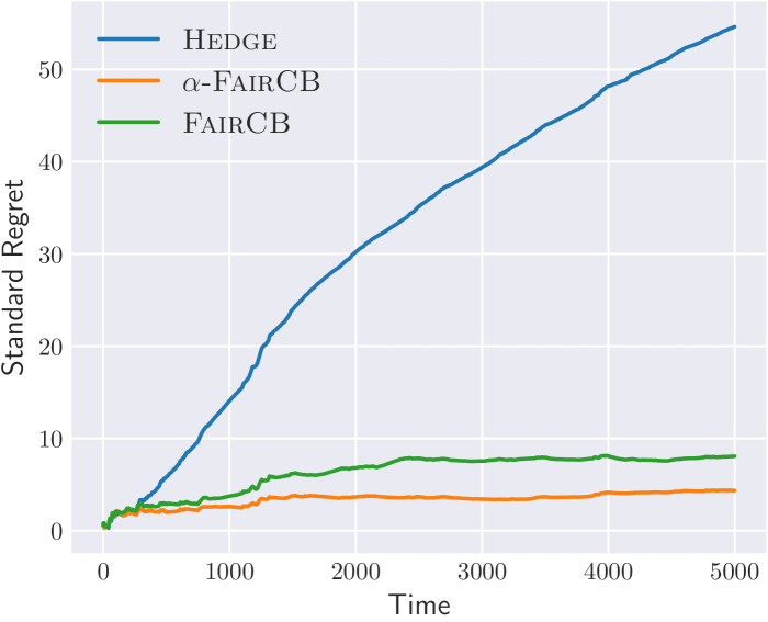
Figure 8: Standard regret for the full information setting.

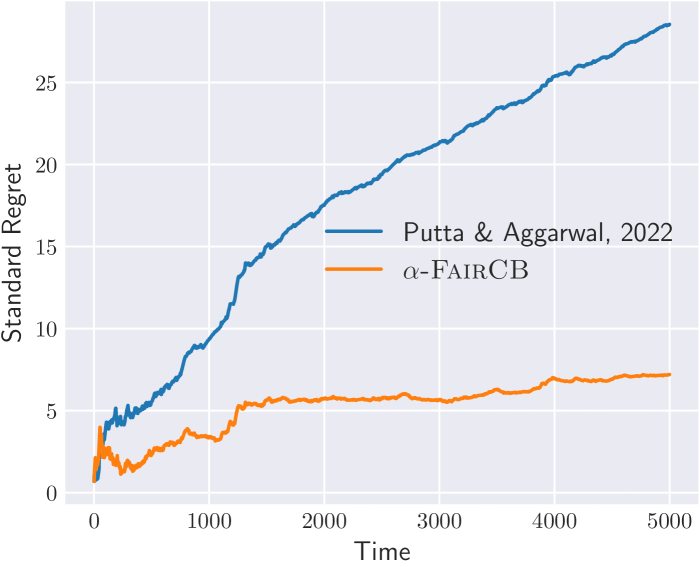
Figure 9: Standard regret for the bandit information setting.

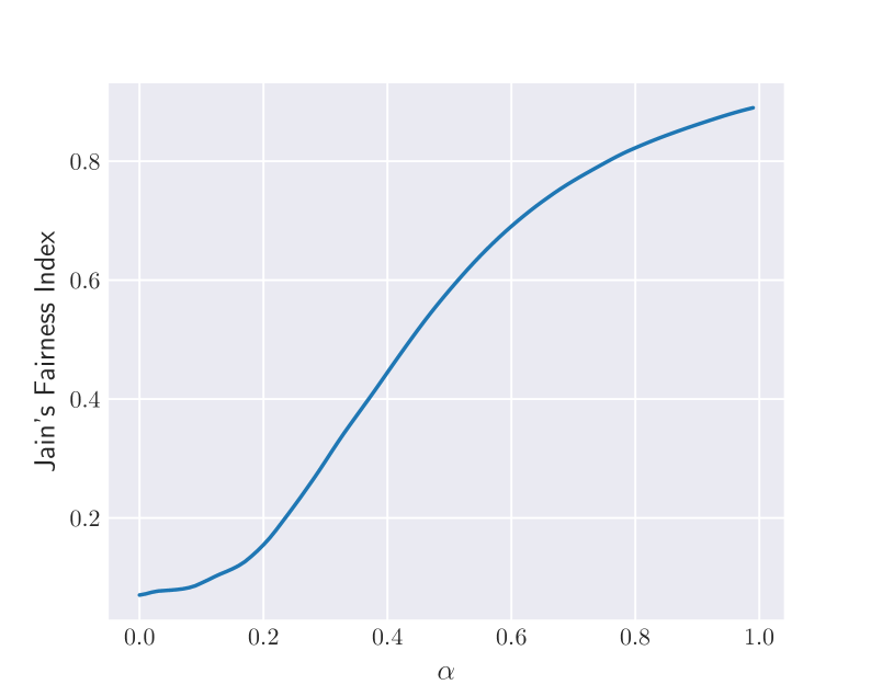
Figure 10: Jain’s Fairness Index for varying values of $\alpha$

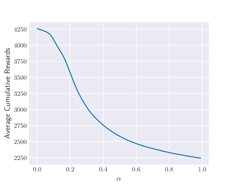
Figure 11: Averaged Cumulative Rewards for varying values of $\alpha$

Figures 9 and 9 show plots of the standard regret of all the policies in the full information and the bandit information settings respectively. As before, it is clearly seen that the $\alpha\textsc{-FairCB}$ policy beats all the other policies in terms of the standard regret in both the settings.

We also run a few experiments to see how varying values of $\alpha$ in the interval $[0,1)$ affects fairness levels in terms of Jain’s Fairness Index (26). Note that the offline benchmark defined by equations (3) and (12) becomes the usual sum of rewards benchmark in the case of $\alpha=0$, i.e it corresponds to an unfair objective. Thus, increasing values of $\alpha$ in the range $[0,1)$ should increase fairness levels. Consequently, the average of cumulative rewards, defined by the equation

$$\text{Average Cumulative Reward}:=\dfrac{\sum_{i\in[N]}R_{i}(T)}{N}$$ (90)

should also decrease as $\alpha$ increases.

For these experiments, we only consider those contexts (users) in the dataset that occur with a high frequency (at least $5000$). In the dataset, there are $M=18$ such contexts, and as before there are $N=19$ arms (genres). In this case, the time horizon was $T=136267$. We again sort the rows of the filtered dataset by timestamps. We took $100$ distinct values of $\alpha$ in the interval $[0,1)$, and trained the $\alpha\textsc{-FairCB}$ policy for each of these values of $\alpha$ in the full information setting. Figure 11 shows a plot of Jain’s Fairness Index achieved by the $\alpha\textsc{-FairCB}$ policy for varying values of $\alpha$ (the index was calculated for the cumulative rewards at the final time step $T$). It is clearly seen that as $\alpha$ increases, the fairness index also increases. Figure 11 shows the average cumulative reward (90, computed at the final time step $T$) and it is observed that as $\alpha$ increases, the average cumulative reward decreases.

References

- Agarwal et al. (2014) Alekh Agarwal, Daniel Hsu, Satyen Kale, John Langford, Lihong Li, and Robert Schapire. Taming the monster: A fast and simple algorithm for contextual bandits. In International Conference on Machine Learning, pages 1638–1646. PMLR, 2014.
- Agrawal and Devanur (2014) Shipra Agrawal and Nikhil R Devanur. Bandits with concave rewards and convex knapsacks. In Proceedings of the fifteenth ACM conference on Economics and computation, pages 989–1006, 2014.
- Agrawal et al. (2016) Shipra Agrawal, Nikhil R Devanur, and Lihong Li. An efficient algorithm for contextual bandits with knapsacks, and an extension to concave objectives. In Conference on Learning Theory, pages 4–18. PMLR, 2016.
- Auer et al. (2002) Peter Auer, Nicolo Cesa-Bianchi, Yoav Freund, and Robert E Schapire. The nonstochastic multiarmed bandit problem. SIAM journal on computing, 32(1):48–77, 2002.
- Azar et al. (2022) Yossi Azar, Amos Fiat, and Federico Fusco. An -regret analysis of adversarial bilateral trade. Advances in Neural Information Processing Systems, 35:1685–1697, 2022.
- Badanidiyuru et al. (2014) Ashwinkumar Badanidiyuru, John Langford, and Aleksandrs Slivkins. Resourceful contextual bandits. In Conference on Learning Theory, pages 1109–1134. PMLR, 2014.
- Celis et al. (2019) L Elisa Celis, Sayash Kapoor, Farnood Salehi, and Nisheeth Vishnoi. Controlling polarization in personalization: An algorithmic framework. In Proceedings of the conference on fairness, accountability, and transparency, pages 160–169, 2019.
- Chen et al. (2020) Yifang Chen, Alex Cuellar, Haipeng Luo, Jignesh Modi, Heramb Nemlekar, and Stefanos Nikolaidis. Fair contextual multi-armed bandits: Theory and experiments. In Conference on Uncertainty in Artificial Intelligence, pages 181–190. PMLR, 2020.
- Claure et al. (2020) Houston Claure, Yifang Chen, Jignesh Modi, Malte Jung, and Stefanos Nikolaidis. Multi-armed bandits with fairness constraints for distributing resources to human teammates. In Proceedings of the 2020 ACM/IEEE International Conference on Human-Robot Interaction, pages 299–308, 2020.
- Diamond and Boyd (2016) Steven Diamond and Stephen Boyd. Cvxpy: A python-embedded modeling language for convex optimization. The Journal of Machine Learning Research, 17(1):2909–2913, 2016.
- Emamjomeh-Zadeh et al. (2021) Ehsan Emamjomeh-Zadeh, Chen-Yu Wei, Haipeng Luo, and David Kempe. Adversarial online learning with changing action sets: Efficient algorithms with approximate regret bounds. In Algorithmic Learning Theory, pages 599–618. PMLR, 2021.
- Even-Dar et al. (2009) Eyal Even-Dar, Robert Kleinberg, Shie Mannor, and Yishay Mansour. Online learning with global cost functions. In 22nd Annual Conference on Learning Theory, COLT, 2009. URL http://www.cs.mcgill.ca/~colt2009/papers/005.pdf#page=1.
- Harper and Konstan (2015) F. Maxwell Harper and Joseph A. Konstan. The movielens datasets: History and context. ACM Trans. Interact. Intell. Syst., 5(4), dec 2015. ISSN 2160-6455. doi: 10.1145/2827872. URL https://doi.org/10.1145/2827872.
- Jain et al. (1998) R. Jain, D. Chiu, and W. Hawe. A quantitative measure of fairness and discrimination for resource allocation in shared computer systems, 1998.
- Joseph et al. (2016) Matthew Joseph, Michael Kearns, Jamie H Morgenstern, and Aaron Roth. Fairness in learning: Classic and contextual bandits. Advances in neural information processing systems, 29, 2016.
- Lan et al. (2010) Tian Lan, David Kao, Mung Chiang, and Ashutosh Sabharwal. An axiomatic theory of fairness in network resource allocation. IEEE, 2010.
- Li et al. (2019) Fengjiao Li, Jia Liu, and Bo Ji. Combinatorial sleeping bandits with fairness constraints. IEEE Transactions on Network Science and Engineering, 7(3):1799–1813, 2019.
- Orabona (2019) Francesco Orabona. A modern introduction to online learning. arXiv preprint arXiv:1912.13213, 2019.
- Paria and Sinha (2021) Debjit Paria and Abhishek Sinha. LeadCache : Regret-optimal caching in networks. Advances in Neural Information Processing Systems, 34:4435–4447, 2021.
- Patil et al. (2021) Vishakha Patil, Ganesh Ghalme, Vineet Nair, and Yadati Narahari. Achieving fairness in the stochastic multi-armed bandit problem. The Journal of Machine Learning Research, 22(1):7885–7915, 2021.
- Putta and Agrawal (2022) Sudeep Raja Putta and Shipra Agrawal. Scale-free adversarial multi armed bandits. In International Conference on Algorithmic Learning Theory, pages 910–930. PMLR, 2022.
- Semenov et al. (2022) Alexander Semenov, Maciej Rysz, Gaurav Pandey, and Guanglin Xu. Diversity in news recommendations using contextual bandits. Expert Systems with Applications, 195:116478, 2022.
- Si Salem et al. (2022) Tareq Si Salem, Georgios Iosifidis, and Giovanni Neglia. Enabling long-term fairness in dynamic resource allocation. Proceedings of the ACM on Measurement and Analysis of Computing Systems, 6(3):1–36, 2022.
- Sinha et al. (2023) Abhishek Sinha, Ativ Joshi, Rajarshi Bhattacharjee, Cameron Musco, and Mohammad Hajiesmaili. No-regret algorithms for fair resource allocation. arXiv preprint arXiv:2303.06396, 2023.
- Slivkins (2011) Aleksandrs Slivkins. Contextual bandits with similarity information. In Proceedings of the 24th annual Conference On Learning Theory, pages 679–702. JMLR Workshop and Conference Proceedings, 2011.