Genetic Algorithms with Neural Cost Predictor for Solving Hierarchical Vehicle Routing Problems

Abstract

When vehicle routing decisions are intertwined with higher-level decisions, the resulting optimization problems pose significant challenges for computation. Examples are the multi-depot vehicle routing problem (MDVRP), where customers are assigned to depots before delivery, and the capacitated location routing problem (CLRP), where the locations of depots should be determined first. A simple and straightforward approach for such hierarchical problems would be to separate the higher-level decisions from the complicated vehicle routing decisions. For each higher-level decision candidate, we may evaluate the underlying vehicle routing problems to assess the candidate. As this approach requires solving vehicle routing problems multiple times, it has been regarded as impractical in most cases. We propose a novel deep-learning-based approach called Genetic Algorithm with Neural Cost Predictor (GANCP) to tackle the challenge and simplify algorithm developments. For each higher-level decision candidate, we predict the objective function values of the underlying vehicle routing problems using a pre-trained graph neural network without actually solving the routing problems. In particular, our proposed neural network learns the objective values of the HGS-CVRP open-source package that solves capacitated vehicle routing problems. Our numerical experiments show that this simplified approach is effective and efficient in generating high-quality solutions for both MDVRP and CLRP and has the potential to expedite algorithm developments for complicated hierarchical problems. We provide computational results evaluated in the standard benchmark instances used in the literature.

Key words: multi-depot vehicle routing problem, genetic algorithm, deep learning, cost prediction

1 Introduction

Vehicle Routing Problems (VRPs) have been extensively studied over the past few decades, owing to their crucial role in last-mile delivery logistics. As a direct extension of the traveling salesman problem, the Capacitated Vehicle Routing Problem (CVRP) is a fundamental VRP class that provides a basis for many VRP variants. In many real-life routing problems, the VRP in focus often includes additional constraints, parameters, or assumptions. Such problems are referred to as VRP variants or rich VRPs.

Among many VRP variants, we focus on hierarchical VRPs, where the upper-level decisions impact the lower-level decisions. Examples include two widely used VRP variants called Multi-Depot VRP (MDVRP) and Capacitated Location Routing Problem (CLRP). In essence, the MDVRP involves the additional task of clustering customers with order-fulfillment centers from where the respective demands are fulfilled. Clustering decomposes the original problem into multiple CVRPs. A simple example is illustrated in Figure 1. Evidently, the MDVRP is at least as difficult as CVRP, and thus an $\mathcal{NP}$-Hard problem. In MDVRPs, the upper-level decisions are the assignment of each customer to a depot, and the lower-level decisions are the routing of vehicles for each depot. As a generalization of MDVRP, CLRP has an additional upper-level decision to be made regarding which depots should be opened from the available candidate locations.

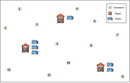
(a) An example MDVRP instance

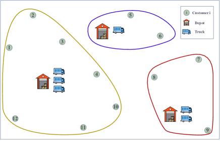
(b) Customer assignments to depots in an MDVRP

Figure 1: A distinct decomposition of MDVRP to VRPs

MDVRP is a fundamental optimization problem in many real-world transportation problems, such as grocery delivery, waste collection, mobile healthcare routing, and field service management. Take the example of an organization that operates a chain of grocery stores or hypermarkets throughout a region. If a customer’s delivery demands can be satisfied from multiple stores, the company needs to decide which store fulfills the customer demand. With several incoming orders from different geographical locations and a limited number of delivery agents available at each store, the organization needs to determine the optimal assignment of each customer to a store such that the overall transportation cost is minimized. It is evident that the allocation of one or more customers to their nearest store, disregarding other factors such as geographical distribution of demands, may lead to suboptimal or even infeasible solutions.

The main challenge in obtaining real-time solutions to combinatorial optimization (CO) problems is their computational complexity. Although heuristics tackle this issue for relatively small and medium-sized problems, the search space for good solutions increases exponentially as the problem size increases. For problems that can be decomposed into “simpler” subproblems, a convenient solution method is to find the optimal decomposition. The objective function value of our original MDVRP with customer-depot assignments is the sum of the optimal costs of all decomposed CVRPs. However, recall that MDVRP decomposition leads to multiple CVRPs that are still $\mathcal{NP}$-Hard. To evaluate a decomposition, the only requirement is the optimal routing cost of each subproblem without the need for routing decisions.

In this paper, we train a deep neural network (NN) model to predict the optimal cost of a given CVRP instance, arising in the decomposition of hierarchical VRPs without actually solving the problem. The predicted cost can be leveraged as an approximate measure of the decomposition strategy’s effectiveness. With the help of a Genetic Algorithm (GA), we improve the clustering of customers with depots. The fitness cost of an assignment is calculated from the sum of the subproblems’ cost and the distinctiveness of the decomposition among other assignments. We refer to this approach as the Genetic Algorithm with Neural Cost Predictor (GANCP).

Our numerical experiments demonstrate that GANCP is effective in obtaining high-quality solutions with outstanding computational advantages. At the final stage of the proposed method, we use the HGS-CVRP solver (Vidal, 2022) to obtain an actual routing solution. Therefore, we refer to our complete end-to-end solution method with the use of the subproblem solver as $\text{GANCP}^{+}$. Test results are compared with the performance of an open-source generic VRP solver, the Vehicle Routing Open-source Optimization Machine (VROOM) (Coupey et al., 2023). In many variants of VRPs, VROOM is known to produce high-quality solutions that are close to the best-known solutions reported in the literature. We analyze the performance of the cost prediction model using three different train data generation procedures. We also showcase the transferability of our heuristic for instances distinct from the trained distribution and range.

We believe that the proposed $\text{GANCP}^{+}$ has the potential to tackle many challenging hierarchical VRPs arising in the real world for the following reasons. First, the trained NN can predict the cost of each candidate quickly. The biggest challenge in the decomposition approach for hierarchical VRPs is the time to solve subproblems. In our approach, we use an NN to obtain a cost prediction in a short amount of time without solving the problem. Second, our proposed NN can learn the cost values from standard VRP solvers for a wide range of problem sizes. Fundamental building blocks in hierarchical VRPs are well-studied problems such as CVRP, for which several outstanding VRP solvers exist. Therefore, we can train an NN for each standard VRP class and use it for various hierarchical VRPs that use the same VRP class of problems as a lower-level decision. This can reduce the algorithm development time significantly, as we can focus on how to handle non-standard modeling components within the GA framework without considering the routing solutions. Third, our proposed NN architecture can provide a robust prediction capability for the same VRP class within different problem contexts. We demonstrate the transferability of the trained NN from MDVRP to CLRP by experimenting with various benchmark datasets.

Our goal in this paper is, therefore, to show that the proposed approach can simplify algorithm development processes for complicated hierarchical vehicle routing problems and produce quality solutions in a short amount of time rather than to develop an algorithm that can produce the best solutions and outperform all existing algorithms. We will focus on illustrating this main point throughout the paper and will use MDVRP and CLRP as examples.

The remainder of this paper is organized as follows. In Section 2, we discuss the relevant literature on CVRP methodologies involving reinforcement learning (RL), machine learning (ML), and heuristics, followed by a brief review of related literature on MDVRP and CLRP. Section 3 describes hierarchical vehicle routing problems in general and discusses the mathematical formulation for CLRP. The neural network prediction model and training details are discussed in Section 4. Section 5 discusses our MDVRP solution methodology with details on the NN model architecture and the heuristics. In Section 6, we briefly discuss the changes to our MDVRP heuristics to solve a CLRP instance. We discuss and evaluate the performance of the NN model using three different training procedures in Section 7. We further demonstrate the effectiveness of our proposed heuristic on multiple MDVRP instances, including out-of-distribution and out-of-range instances. Section 8 discusses the results of the CLRP experiments. The paper finally concludes with a discussion of relevant and related research directions in optimization using supervised learning in Section 9.

2 Literature Review

First, we review the relevant literature on VRPs that use deep RL as a solution methodology. This follows a review of relevant research on solution methods for MDVRP and CLRP. Finally, we highlight our contribution to the existing research gap.

2.1 Deep Reinforcement Learning Approaches for VRPs

Over the past few years, deep reinforcement learning has been demonstrating notable success in solving combinatorial optimization problems, especially TSP and CVRP. Bello et al. (2017) introduces an efficient deep RL framework to train and solve the Traveling Salesman Problem using Pointer Networks by Vinyals et al. (2015). The problem is modeled as a Markov Decision Process and uses the pointer network for encoding the inputs, which are then learned using policy gradients. Nazari et al. (2018) extends this work for VRPs without a Recurrent Neural Network for input encoding. Unlike Natural Language Processing, the order of the input sequence—the customer locations—can be treated independently in VRP. While the inclusion of a pointer encoder network does not negatively impact the final accuracy, it delays learning due to added model complexity. Kool et al. (2019) yields better performance for CVRPs using an architecture for solution construction with multiple multi-head attention layers, proposed in Vaswani et al. (2017), to capture the node dependencies and REINFORCE algorithm to train the model. With consideration of symmetries in the solutions of a CO problem, Kwon et al. (2020) designs the Policy Optimization with Multiple Optima (POMO) network with a modified REINFORCE algorithm to explore the solution space more effectively. This improves the results in terms of both optimality gap and inference time compared to the existing architectures. All of these approaches are end-to-end solution approaches that rely solely on neural networks to solve the problem.

Traditional end-to-end RL frameworks for CO solution construction have limitations concerning the scope and size of the problems they can effectively address. Another active research focus is on the use of RL as an enhancement heuristic for problem partitions or when an initial solution is known. Li et al. (2021) proposes a method that iteratively improves the solution to large-scale VRPs by learning to select subproblems and estimating the corresponding subsolution costs using a transformer architecture. Using a combination of a subproblem selector and cost estimation, the problem can be partitioned into smaller problems that are easily solved. Zong et al. (2022) proposes a Rewriting-by-Generating framework for solving large-scale VRPs hierarchically. Here, the Rewriter agent partitions the customers into independent regions, and the Generator agent solves the routing problem in each region. This method outperforms a widely used CVRP solver by Vidal (2022) for large-scale problems, where the hyperparameters are fine-tuned for small to medium-size CVRP problems. Kim et al. (2023) proposes a neural cross-exchange operator to solve multiple VRP variants with reduced computational complexity than the traditional operator. The results of these studies demonstrate the effectiveness of supervised learning in solving large-scale routing problems. Unlike end-to-end approaches that learn routing solutions, these improvement approaches learn potential cost improvements for a subproblem. This stream of research motivates our proposed approach in this paper.

2.2 Optimization Approaches for MDVRP and CLRP

Multiple studies use exact methods to solve MDVRP, such as Laporte et al. (1988), Contardo and Martinelli (2014), and Baldacci and Mingozzi (2009). Similarly, for the study of CLRP using exact methods, please refer to Baldacci et al. (2011), Belenguer et al. (2011) and Contardo et al. (2014). As a consequence of the $\mathcal{NP}$-hardness of these problems, efficient heuristics are critical to the development of industrial routing solutions.

Cordeau et al. (1997) proposes a notable Tabu Search (TS) heuristic to solve MDVRP, Periodic VRP, and the Periodic Traveling Salesman Problem. A few years later, genetic algorithms emerged as one of the most effective routing heuristics. Vidal et al. (2012) proposes a fast and efficient hybrid genetic algorithm that solves MDVRP and Periodic VRP. The algorithm differentiates neighboring solutions using a diversity factor in fitness cost. In addition, a pool of infeasible solutions is preserved for diversification and better search space. Vidal et al. (2014) further improves the results where the depot, vehicle, and first customer visited on each route are optimally determined using a dynamic programming methodology. Sadati et al. (2021) presents a Variable Neighborhood Search algorithm that solves MDVRP variants with a tabu-shaking mechanism to improve the search trajectory. End-to-end RL frameworks for MDVRP are presented in Zou et al. (2022) based on an improved transformer model and Zhang et al. (2023) using Graph Attention Networks.

One of the most effective existing algorithms for solving large-scale CLRP is by Schneider and Löffler (2019), which explores multiple depot configurations using a Tree-Based Search Algorithm (TBSA). For a given configuration, an MDVRP is solved at the routing phase using a granular tabu search. The paper also discusses different variants of the algorithm with trade-offs in computational time and solution quality. More recently, Akpunar and Akpinar (2021) proposes a Hybrid Adaptive Large Neighborhood Search method that demonstrates improved benchmark performance in a few CLRP benchmark instances.

Our $\text{GANCP}^{+}$ heuristic is empowered with a supervised learning model for cost estimation, which requires less training time and is more importantly applicable to distinct and large problem sizes producing near-optimal results. To the best of our knowledge, this paper is the first to address solving large-scale hierarchical VRPs using a deep learning architecture to evaluate subproblem decompositions.

3 Hierarchical Vehicle Routing Problems

Hierarchical vehicle routing problems (HVRPs) involve decisions made at multiple levels, often executed sequentially, to obtain an optimal routing solution. A large instance or a complex problem can be decomposed into smaller subproblems by breaking HVRPs into multiple levels of decision-making and finding effective upper-level decisions in consideration of the original problem constraints and the objective function. Higher-level decisions influence subsequent decisions, solution quality, and the optimal objective cost of the original problem. Lower-level decisions include detailed vehicle routing and schedule plans to complete deliveries or services for each vehicle.

As the HVRPs require decisions in addition to and including vehicle routing, it is computationally challenging to solve such problems in many real-life scenarios. In this paper, we focus on two widely applicable HVRP variants, MDVRP and CLRP. Due to the complexity of the HVRPs, multiple techniques and their combination are often used to solve large instances. A straightforward approach is to focus on the method to find effective upper-level decisions and solve the corresponding subproblems using an existing efficient algorithm or a proven solver. The upper-level decisions decompose the MDVRPs and CLRPs into subsequent CVRPs, where the total solution cost determines the quality of the upper-level decisions. Because VRPs are well-researched, we focus on a heuristic method to find higher-level decisions for MDVRPs and CLRPs.

We examine the Mixed Integer Linear Programming formulation of the CLRP, as proposed in Laporte et al. (1986), in this section. Since CLRP is a generalization of MDVRP, the formulation can be easily extended to MDVRP by eliminating the additional assumptions. We consider a complete and undirected graph $\mathcal{G}=(\mathcal{V},\mathcal{E})$. Let $\mathcal{V}$ be the set of all nodes, $\mathcal{D}\subset\mathcal{V}$ be the set of potential depots, and $\mathcal{E}$ denote the set of all edges that connect nodes in $\mathcal{V}$. Each demand location $i\in\mathcal{V}\setminus\mathcal{D}$ has a positive demand $q_{i}$ such that $q_{i}\leq Q$, where $Q$ is the vehicle capacity of a homogeneous fleet of vehicles. Number of vehicles or routes $m_{d}$ used from a depot $d$ lies within a given bound: $m_{d}\in[0,\mkern 1.5mu\overline{\mkern-1.5mum\mkern-1.5mu}\mkern 1.5mu_{d}]$. Similarly, the number of depots opened in the optimal solution also lies within a specified bound of potential depots, i.e., $[\underline{$D$},\mkern 1.5mu\overline{\mkern-1.5muD\mkern-1.5mu}\mkern 1.5mu]$ where $\underline{$D$}\geq 1$ and $\mkern 1.5mu\overline{\mkern-1.5muD\mkern-1.5mu}\mkern 1.5mu\leq|\mathcal{D}|$. For MDVRP and some VRP variants, the number of depots to be opened is exactly the number of depots given in the instance.

An assumption follows in CLRP that vehicles that start from a depot must return to the same depot after services. Opening of a depot $d$ and a route corresponding to depot $d$ results in depot opening cost $c^{D}_{d}$ and vehicle opening cost $c^{V}_{d}$, respectively. In addition, consider $\mathcal{S}\subset\mathcal{V}\setminus\mathcal{D}$ for subtour elimination. Let $x_{ij}$ be an integer decision variable representing the number of times the edge $(i,j)$ is traversed in the optimal solution, and we assume $i<j$. Since the edges are undirected, $x_{ij}$ should be represented as $x_{ji}$ when $j>i$. The traversal cost for the edge $(i,j)$ is denoted as $c_{ij}$, where $c_{ij}=c_{ji}$. We assume that the costs associated with edges adhere to the triangle inequality. Opening of a potential depot is indicated by the binary decision variable $y_{d}$, where $d\in\mathcal{D}$. The problem is then formulated as follows:

$$\min z= \sum_{d\in\mathcal{D}}(c^{D}_{d}y_{d}+c^{V}_{d}m_{d})+\sum_{i,j\in\mathcal{V}}c_{ij}x_{ij}$$ (1)

$$\sum_{i<k}x_{ik}+\sum_{k<j}x_{kj}=2 \forall k\in\mathcal{V}\setminus\mathcal{D}$$ (2)

$$\sum_{i<d}x_{id}+\sum_{d<j}x_{dj}=2m_{d} \forall d\in\mathcal{D}$$ (3)

$$\sum_{i,j\in\mathcal{S}}x_{ij}\leq|\mathcal{S}|-\left\lceil\frac{\sum_{k\in\mathcal{S}}q_{k}}{Q}\right\rceil \mathcal{S}\subseteq\mathcal{V}\setminus\mathcal{D}:|\mathcal{S}|\geq 3$$ (4)

$$x_{i_{1},i_{2}}+3x_{i_{2},i_{3}}+x_{i_{3},i_{4}}\leq 4 \forall i_{1},i_{4}\in\mathcal{D};i_{2},i_{3}\in\mathcal{V}\setminus\mathcal{D}$$ (5)

$$x_{i_{1},i_{2}}+x_{i_{h-1},i_{h}}+2\sum_{i,j\in\{i_{2},\dots,i_{h-1}\}}x_{ij}\leq 2h-5 \forall h\geq 5;i_{1},i_{h}\in\mathcal{D};i_{2},\dots,i_{h-1}\in\mathcal{V}\setminus\mathcal{D}$$ (6)

$$0\leq m_{d}\leq\mkern 1.5mu\overline{\mkern-1.5mum\mkern-1.5mu}\mkern 1.5mu_{d}y_{d} \forall d\in\mathcal{D}$$ (7)

$$\underline{$D$}\leq\sum_{d\in\mathcal{D}}y_{d}\leq\mkern 1.5mu\overline{\mkern-1.5muD\mkern-1.5mu}\mkern 1.5mu$$ (8)

$$y_{d}\in\{0,1\} \forall d\in\mathcal{D}$$ (9)

$$x_{ij}\in\{0,1\} \forall i,j\in\mathcal{V}\setminus\mathcal{D}$$ (10)

$$x_{ij}\in\{0,1,2\} \forall i\text{ or }j\in\mathcal{D}$$ (11)

The objective function (1) is to minimize the total cost of the solution, inclusive of depot and vehicle opening costs as well as the routing costs. Constraint (2) ensures that each customer is visited exactly once in the optimal solution. Similarly, constraint (3) indicates that exactly $m_{d}$ vehicles must leave and return to the depot $d$. Subtour elimination constraint is presented in (4), which further ensures that the vehicle capacities are not violated. Constraints (5), (6) are referred to as chain-barring constraints, and they ensure that the vehicles start and end their journey at the same depot. For a detailed explanation of these results, readers are referred to Laporte et al. (1986). Constraint (7) specifies the bounds for the number of opened routes associated with a depot, and the binary decision variable is positive only if at least one vehicle is used from a depot. Similarly, the given bounds in the number of depots to be opened, if any, is given in constraint (8). From constraint (9), if the decision variable $y_{d}=1$, the depot at location $d$ is opened and $y_{d}=0$, otherwise. Constraints (10), (11) determines the number of trips in an arc $(i,j)$ corresponding to the decision variable $x_{ij}$. Here, $x_{ij}=2$ denotes a return trip between $i$ and $j$ after a single service. In some scenarios, each depot $d\in\mathcal{D}$ has a capacity $U_{d}$. Then, the total demand satisfied by the depot is bounded by $y_{d}U_{d}$. The MDVRP, as defined in Cordeau et al. (1997), does not have depot capacities, depot costs, and vehicle opening costs.

We will now examine the decomposition of the CLRP model in (1)–(11) to VRP subproblems. For a given instance, let us consider a partial feasible solution $\hat{y}=(\hat{y}_{d})_{d\in\mathcal{D}}$ such that the constraints (8) and (9) are satisfied. With a collection of all depots $d$ where $\hat{y}_{d}=1$, the problem reduces to an MDVRP with the depot set $\tilde{\mathcal{D}}\subseteq\mathcal{D}$. This is evident from the above CLRP formulation.

Next, if we assign the customers distinctly to the depots in $\tilde{\mathcal{D}}$, we obtain at most $\sum_{d\in\mathcal{D}}\hat{y}_{d}=|\tilde{\mathcal{D}}|$ non-empty CVRPs. Let $\mathcal{V}^{P}=\{\mathcal{V}_{1},\mathcal{V}_{2},\dots,\mathcal{V}_{|\tilde{\mathcal{D}}|}\}$ be a partition of $\mathcal{V}\setminus\mathcal{D}$ such that $\mathcal{V}\setminus\mathcal{D}=\mathcal{V}_{1}\cup\mathcal{V}_{2}\cup\cdots\cup\mathcal{V}_{|\tilde{\mathcal{D}}|}$ and $\mathcal{V}_{i}\cap\mathcal{V}_{j}=\emptyset$ for $1\leq i<j\leq|\tilde{\mathcal{D}}|$ and $i\neq j$. With an one-to-one mapping $\hat{\rho}:\{1,2,...,|\tilde{\mathcal{D}}|\}\mapsto\{1,2,...,|\mathcal{D}|\}$, this partition represents the assignment of customers to $|\tilde{\mathcal{D}}|$ out of $|\mathcal{D}|$ depots. We assume that the partition is ordered so that $\mathcal{V}_{d}$ is served by depot $d$. If $|\mathcal{D}|-|\tilde{\mathcal{D}}|\geq 1$, there exists at least one depot that does not have customers to service. In this case, the upper-level decisions comprise the opening of depots, followed by the assignment of customers to each depot that has been opened. It is assumed that the customer assignments are carefully executed to ensure compliance with vehicle capacity and fleet number constraints for each depot. Given a feasible $\mathcal{V}^{P}$, we denote the resultant VRP subproblem for each depot $d\in\tilde{\mathcal{D}}$ and corresponding set of parameters $\phi_{d}$ as $\mathsf{VRP}(\mathcal{V}_{d};\phi_{d})$ with the following formulation:

$$\min_{x,m_{d}}\quad c^{D}_{d}+c^{V}_{d}m_{d}+\sum_{i,j\in\mathcal{V}_{d}}c_{ij}x_{ij}$$ (12)

$$\sum_{i<k}x_{ik}+\sum_{k<j}x_{kj}=2 \forall k\in\mathcal{V}_{d}$$ (13)

$$\sum_{i<d}x_{id}+\sum_{d<j}x_{dj}=2m_{d}$$ (14)

$$\sum_{i,j\in\mathcal{S}}x_{ij}\leq|\mathcal{S}|-\left\lceil\frac{\sum_{k\in\mathcal{S}}q_{k}}{Q}\right\rceil \mathcal{S}\subseteq\mathcal{V}_{d}:|\mathcal{S}|\geq 3$$ (15)

$$0\leq m_{d}\leq\mkern 1.5mu\overline{\mkern-1.5mum\mkern-1.5mu}\mkern 1.5mu_{d}$$ (16)

$$x_{ij}\in\{0,1\} \forall i,j\in\mathcal{V}_{d}$$ (17)

$$x_{dj},x_{jd}\in\{0,1,2\} \forall j\in\mathcal{V}_{d}$$ (18)

It can be noticed that the chain barring constraints are missing in the above VRP subproblem. Constraints (5), (6) are defined using two distinct depots $i_{1},i_{4}\in\mathcal{D}$ or $i_{1},i_{h}\in\mathcal{D}$, respectively. In the decomposition of CLRP to multiple VRPs using upper-level decisions $\hat{y}$, these constraints are no longer present. The above reduction of CLRP into subsequent subproblems is to demonstrate the mathematical accuracy of using our decomposition strategy in HVRPs. For the MDVRP and CVRP instances considered in this study, $c^{D}_{d}=0$ and $c^{V}_{d}=0$. Therefore, the CVRP prediction model is trained to predict only the optimal routing cost. To simplify the prediction model, we assume that there is no upper bound in the number of vehicles for the CVRP instances. When vehicle opening costs are involved, i.e., in CLRP instances, we approximate $m_{d}$ to evaluate a decomposition. However, the costs are calculated near-optimal in the final step.

In general, many VRP variants can be decomposed into VRP subproblems as above, such as Periodic VRP, MDVRP, Periodic MDVRP, Split Delivery VRP, etc. Suppose $\hat{x}_{d}$ be an optimal solution to $(\mathcal{V}_{d};\phi_{d})$ such that $\hat{x}=(\hat{x}_{d})_{d\in\mathcal{D}}$, and let a function $P(\cdot)$ calculate the total routing cost for a given route.

$$P(\hat{x})=P(\hat{x}_{1})+P(\hat{x}_{2})+\dots+P(\hat{x}_{|\tilde{\mathcal{D}}|})$$ (19)

$P(\hat{x})$ gives the total optimal routing cost for the original HVRP, subject to parameters $\phi$ used in the subproblems, and can be used as a measure to evaluate the upper-level decisions in association with the costs corresponding to depot and vehicle opening costs, say $R(\hat{y},\hat{x})$.

Although this is a direct decomposition approach, there has been limited research on related methodologies due to the challenge of evaluating multiple decomposition strategies by addressing several subproblems. Our solution to this issue involves training a supervised learning network to predict the optimal routing cost of a CVRP based on the input graph structure. Since the neural network is trained only to predict the near-optimal cost, rather than the actual routing solution, we benefit from significant computational advantages. Consequently, to evaluate upper-level decisions, we need $P(x)$ and do not directly require $x\in\mathcal{X}$. The next section discusses the neural network architecture used to approximate the optimal cost of a subproblem.

4 Learning to predict CVRP Costs

For a formal definition of our CVRP training instances, consider the complete and undirected graph $\mathcal{G}=(\mathcal{V},\mathcal{E})$ defined in Section 3, with $|\mathcal{V}|=N+1$ and the cardinality of depot set $|\mathcal{D}|=1$. Each customer $i$ has a positive demand denoted as $q_{i},i=1,2,\dots,N$. The objective of CVRP is to find the minimum total cost for all routes where each route is traversed by one of the fixed number of homogeneous vehicles, each with a capacity of $Q$, satisfying the following conditions:

• Each route must start and end at the depot.

• Each customer must belong to exactly one route.

• The total demand of customers assigned to a route must not exceed the vehicle capacity $Q$.

An effective and widely used heuristic method for this problem is Hybrid Genetic Search (HGS) for CVRP by Vidal (2022), which has an open-source implementation. HGS-CVRP solver remains a top-performing metaheuristic in terms of methodological simplicity, solution quality, and convergence speed. Among the features of this solver is the ability to specify a time limit that restricts the run time of large problems. In the following section, we describe how we predict the near-optimal CVRP cost using a graph neural network (GNN). For model simplicity, we do not explicitly consider the number of vehicles available at a depot as an input parameter. Instead, the network learns to predict the optimal solution cost by analyzing the vehicle capacity, thus indirectly estimating the number of vehicles required. The feasibility of CVRP decomposition, however, is analyzed approximately in light of the total demand, vehicle capacity, and the number of available vehicles. An overview of the prediction model is presented in Figure 2. The GNN is trained to predict optimal CVRP cost, estimated by HGS.

4.1 Predict Cost of CVRP using Graph Neural Network

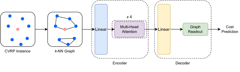
Figure 2: NN architecture

The cost-prediction GNN $f_{\theta}$ predicts the optimal cost of a CVRP instance $\mathcal{G}$ as follows:

$$\mathcal{G}_{\text{knn}} \approx\mathcal{G},$$ (20)

$$\hat{v} =f_{\theta}(\mathcal{G}_{\text{knn}}),$$ (21)

where $\mathcal{G}_{\text{knn}}$ is the graph representation of $\mathcal{G}$ constructed by the k-nearest neighbor (KNN) method, $f_{\theta}$ is the cost-prediction GNN with parameters $\theta$ which will be discussed in the following sections, and $\hat{v}$ is the predicted optimal cost of $\mathcal{G}$.

KNN graph construction

The KNN graph, denoted as $\mathcal{G}_{\text{knn}}$, is constructed by connecting each node to its $k$ nearest neighbors based on the Euclidean distance between the nodes. The node features $U$ consists of two components: normalized node coordinates and normalized demand.

• The normalized node coordinates of $\mathcal{G}_{\text{knn}}$ are computed by translating the node coordinates to ensure they are positive. This is achieved by adding the absolute value of the minimum coordinate values and then dividing them by the maximum coordinate value.

• The normalized demand is defined as the ratio of the demand $q_{i}$ to the vehicle capacity $Q$.

Graph Neural Network Architecture

The cost-prediction GNN $f_{\theta}$ is composed of the encoder, a stack of self-attention blocks (Vaswani et al., 2017), and the decoder, a linear layer followed by the graph readout module. $f_{\theta}$ predicts the cost as follows:

$$\hat{v}=f_{\theta}(\mathcal{G}_{\text{knn}})\coloneqq\texttt{Decoder}(\texttt{Encoder}(\mathcal{G}_{\text{knn}})),$$ (22)

where $\texttt{Encoder}(\cdot)$ and $\texttt{Decoder}(\cdot)$ are described in the following paragraphs.

The $\texttt{Encoder}(\cdot)$ operator transforms $\mathcal{G}_{\text{knn}}$ into the latent vectors $U^{\prime}\in\mathbb{R}^{(N+1)\times h}$, where $N+1$ represents the number of nodes (i.e., customers and depot), and $h$ denotes the hidden node feature dimension. This transformation is achieved through a series of operations.

First, a linear embedding layer is applied to match the input node feature dimension $\tilde{d}$ to $h$. Then, multiple self-attention blocks are employed. Each self-attention block consists of two steps: $\texttt{MultiHeadAttention}(\cdot)$ and $\texttt{FeedForward}(\cdot)$.

The $\texttt{MultiHeadAttention}(\cdot)$ step is defined as follows:

$$\texttt{MultiHeadAttention}(U) =\text{Concat}(\text{head}_{1},\dots,\text{head}_{H})\cdot W^{O}$$ (23)

$$\text{head}_{i} =\texttt{Attention}(U)$$ (24)

In the above equations, $W^{O}\in\mathbb{R}^{H\times h}$ is a learnable parameter, and $\text{head}_{i}$ denotes the attention applied to $U$. The $\texttt{Attention}(\cdot)$ transformation is applied to each node $u_{i}$ in $U$ to compute the updated node feature $u^{\prime}_{i}$:

$$u^{\prime}_{i}=\sum_{j\in\mathcal{N}(i)}\underset{j\in\mathcal{N}(i)}{\text{{softmax}}}\left(\frac{W^{Q}u_{i}\cdot W^{K}u_{j}}{\sqrt{h}}\right)\cdot W^{V}u_{j}$$ (25)

Here, $W^{Q}$, $W^{K}$, and $W^{V}\in\mathbb{R}^{h\times h}$ are learnable parameters, $\mathcal{N}(i)$ represents the set of neighbors of node $i$, and softmax denotes the softmax function applied over $j\in\mathcal{N}(i)$. After the Multi-Head Attention step, the updated node features $U^{\prime}$ are obtained. The attention mechanism is applied to the neighbors of each node, and the attention weights are computed based on the similarity between the node features. This approach allows the encoder to capture the local relationships between the nodes.

After accounting for the local relationships between the nodes, $\texttt{Encoder}(\cdot)$ applies $\texttt{FeedForward}(\cdot)$ to process nodes independently. The $\texttt{FeedForward}(\cdot)$ operator is a multilayer perceptron model applied to each node feature. The updated node features $U^{\prime}$ are computed as follows:

$$U^{\prime} =\texttt{{FeedForward}}(U^{\prime})$$ (26)

To summarize, $\texttt{Encoder}(\cdot)$ consists of the following steps:

$$U^{\prime} =\texttt{{LayerNorm}}(U+\texttt{{MultiHeadAttention}}(U))$$ (27)

$$U^{\prime} =\texttt{{LayerNorm}}(U^{\prime}+\texttt{{FeedForward}}(U^{\prime}))$$ (28)

where the residual connections (He et al., 2016) and normalization layer, $\texttt{LayerNorm}(\cdot)$ (Ba et al., 2016), are applied to attain better trainability of the deep models.

The $\texttt{Decoder}(\cdot)$ operator then transforms the latent vectors $U^{\prime}$ into the predicted optimal cost $\hat{v}$ by applying the graph readout module followed by a linear layer. $\texttt{Decoder}(\cdot)$ is defined as follows:

$$\hat{v}=W\bigg{(}\underbrace{\sum_{i\in\mathcal{N}}\underset{i\in\mathcal{N}}{\text{{softmax}}}\left(u^{\prime}_{i}\right)u^{\prime}_{i}}_{\text{graph readout}}\bigg{)}+b,$$ (29)

where $\mathcal{N}$ represents the set of nodes in $\mathcal{G}_{\text{knn}}$, softmax is applied over the nodes, and $W\in\mathbb{R}^{h\times 1}$ and $b\in\mathbb{R}^{1}$ are the linear projection parameters.

The graph readout module computes the weighted sum of the latent vectors $U^{\prime}$, where the weights are computed based on the similarity between the latent vectors. This approach allows the decoder to capture the global relationships between the nodes. And then, the linear projection is performed to predict the optimal cost.

4.2 Training

Existing CVRP benchmark datasets are insufficient in quantity to train this model, and thus, based on the problem requirements, CVRP instances need to be generated and solved to optimality (or near-optimality) to form the training data. Moreover, the batch processing capability of the deep learning model can be used to our advantage to simultaneously process multiple CVRPs. We use the simple yet effective mean squared error as our loss function.

$$L(\theta,U)=(f_{\theta}(\mathcal{G}_{\text{knn}})-f_{\text{solver}}(\mathcal{G}))^{2}$$

Due to input data normalization, the final cost from average pooling needs to be rescaled by a corresponding factor to obtain the final cost prediction of the CVRP instance.

5 Solution Methodology for MDVRP

In this section, we propose our solution methodology to solve large-scale MDVRPs that involve the decomposition of the original problem into different CVRP subproblems. This approach aims to determine the optimal decomposition of the MDVRP into subsequent subproblems, where each CVRP instance corresponds to a depot of the main problem. Using an effective decomposition strategy, the desired CVRP subproblems can be obtained and solved using any existing method or solver. As CVRPs have been extensively studied, we do not attempt to develop a novel method for solving them. Instead, we utilize a well-established and validated heuristic solver to arrive at the final solution. An evaluation of all possible decomposition strategies could be computationally intractable. Therefore, we first select a set of random customer assignment strategies and improve them iteratively with a simplified genetic algorithm. Note that evaluating each MDVRP decomposition in the GA with an existing VRP solver is computationally expensive and it defeats our goal of solving MDVRPs more effectively than the existing methods in the literature. With a supervised deep learning model, we predict the optimal routing cost of a CVRP instance almost instantly without actually solving it.

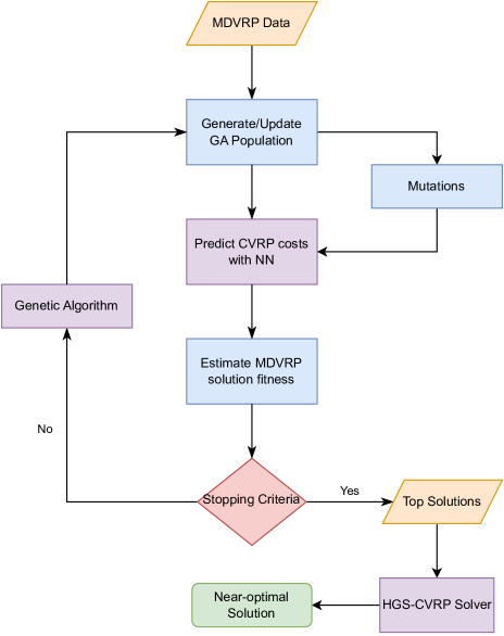
Figure 3: An outline of $\text{GANCP}^{+}$

An outline of our methodology is illustrated in Figure 3. The following sections will discuss the main components of our $\text{GANCP}^{+}$ heuristic, such as genetic algorithm, fitness estimation, and obtaining a final routing solution.

5.1 Genetic Algorithm for MDVRP decomposition

Figure 4: Chromosome representation of customer allocations to depots $\{1,2,3\}$

As an evolutionary approach, GAs represent possible solutions as a set of chromosomes that evolve towards optimality through a process of parent selection, crossover, and mutation over multiple generations. To apply GA, each chromosome is encoded as a string of data. We represent each individual as an $N$-length chromosome of depot allocations that corresponds to customers $i\in\{1,2,\dots,N\}$, as depicted in Figure 4. The customer indices with the same depot allocation $d$ are selected to form the CVRP with depot $d$.

Our algorithm begins with generating an initial population that consists of multiple MDVRP decompositions. Random assignments of customers to depots generate a diverse initial population, and it ensures that the population starts at a high level of diversity, leading to a larger solution search space over time. Besides this rule, we also initialize two to three potential solutions based on the input graph structure. Our study found that a combination of targeted and random assignments in the initial population results in faster algorithm convergence. One of the targeted assignment strategies includes customer allocation to the nearest depot. The second strategy is to allocate each customer to the closest neighbor’s nearest depot. These initial assignment rules have been discussed in de Oliveira et al. (2016). Additionally, we initialize a chromosome where customers are allocated to their second nearest depot for problems with more than two depots. Targeted assignments serve as an effective initial solution to problems involving uniform customer distribution in a region. Metaheuristics can improve such initial solutions and achieve near-optimal results. Random or targeted assignments may, however, provide infeasible candidates with a vehicle capacity that exceeds its total demand, subject to a limited number of vehicles available at the depot. Such individuals could be repaired by selecting a random customer from the infeasible CVRP and reassigning it to a depot that can fulfill the corresponding demand.

Algorithm 1 $\text{GANCP}^{+}$

1:$\Omega\leftarrow\emptyset$ $\triangleright$ Feasible and Infeasible Population

2:$\Omega=\texttt{initial\_population()}$

3:$\texttt{repair\_infeasibles}(\Omega)$

4:$\hat{S}=\texttt{fitness\_scores}(f_{\theta},\Omega)$

5:while number of generations $<N_{\textsc{G}}$ do

6:     $\Omega_{\textsc{sub}}=\texttt{sub\_population}(\Omega,\hat{S},P_{\textsc{l}})$ $\triangleright$ Subpopulation

7:     $\texttt{repair\_infeasibles}(\Omega_{\textsc{sub}})$

8:     $\hat{S}=\texttt{fitness\_scores}(f_{\theta},\Omega_{\textsc{sub}})$

9:     $\Omega_{\textsc{sub}}\leftarrow\texttt{mutations}(\Omega_{\textsc{sub}},\hat{S},\textsc{elite})$

10:     $\hat{S}=\texttt{fitness\_scores}(f_{\theta},\Omega_{\textsc{sub}})$

11:     $\Omega=\texttt{top\_candidates}(\Omega_{\textsc{sub}},\hat{S},\Omega,P_{\textsc{H}})$

12:end while

13:$\texttt{evaluate\_best\_candidates}(\Omega,\texttt{CVRP\_Solver})$

14:Return $\texttt{best\_solutions}()$

Algorithm 2 Repair Infeasible Assignments

1:for $\omega$ in $\Omega$ do $\triangleright$ Infeasible candidate

2:     $r\leftarrow\texttt{rand}(0,1)$

3:     if $r<p_{\textsc{repair}}$ then

4:         while $\omega$ is infeasible assignment do

5:              Find $\texttt{VRP}_{\omega,\textsc{INF}}$ with sum(demands) > sum(vehicle_capacities) $\triangleright$ Infeasible VRP

6:              Randomly remove customer $i$ in $\texttt{VRP}_{\omega,\textsc{INF}}$

7:              Find $\texttt{VRP}_{\omega,\textsc{F}}$ with sufficient remaining capacity. $\triangleright$ Feasible VRP

8:              $\texttt{VRP}_{\omega,\textsc{F}}\leftarrow\texttt{VRP}_{\omega,\textsc{F}}\cup i$

9:         end while

10:     end if

11:end for

12:Return $\Omega$

The next generation of the population is propagated using multiple iterations. At each iteration, two distinct parents are selected from the current solution pool based on fitness scores using a $K$ tournament selection method. As larger tournament sets select better chromosomes but require more computation and may result in premature convergence, we use the binary tournament selection procedure. To generate children, uniform crossover operations are performed over the selected parents by randomly selecting offspring genes from the corresponding genes of the parents. Our simple chromosome representation requires minimal information about the routing solution, so more sophisticated crossover operations are not necessary. The population size is maintained in the range $[P_{L},P_{H}]$. Mutations are performed once crossover operations have generated $P_{L}$ chromosomes for the next generation.

Mutations include the random reset of a customer’s depot, called FLIP, and the SWAP operation, in which two selected customers’ depots are interchanged. Based on their fitness score, chromosomes in the first tertile are selected for mutation. Approximately $5\%$ of all customers undergo a mutation, resulting in either a FLIP or SWAP operation with a probability of $p_{m}$ or $1-p_{m}$. Additional targeted mutations are also carried out over $5\%$ of the child population using a binary tournament selection process. As part of targeted mutations, $10\%$ of the customers are randomly selected, and the depot allocations of these individuals are copied from one of the elite individuals within the initial population of targeted assignments.

5.2 NN Estimation and Fitness function

A candidate solution generated by the GA should be evaluated using a measure of fitness to guide the population toward the direction of minimum cost. In MDVRP, the solution cost is simply the sum of the optimal routing costs for its CVRP subproblems. These costs are predicted using the NN prediction model trained with parameters $\theta$. Although our objective is to minimize the routing cost of the main problem, the application of the MDVRP cost directly as a measure of fitness may lead to premature convergence. With a score for the diversity of a solution in the population, in addition to the predicted cost, which measures solution quality, the GA expands its search space and often overcomes local optima. Hence, the fitness of an individual is calculated using the weighted difference between the predicted MDVRP cost and the diversity factor. In addition, there is a penalty when the assignment is an infeasible decomposition. As seen in (32), normalized solution cost $\tilde{C}$ and normalized diversity factor $\tilde{\delta}$ are used to calculate the fitness score $\text{fit}(I)$ of chromosome $I$. Here, $l_{d}$, $m_{d}$, and $Q$ represent the total demand, the number of available vehicles, and homogeneous vehicle capacity at the depot $d$, respectively. The diversity factor of a chromosome is measured as the mean Hamming distance of the individual from the rest of the population, as shown in (30).

$$\delta(I) =\frac{1}{N|\Omega|}\sum_{\begin{subarray}{c}I^{\prime}\in\Omega\\ I^{\prime}\neq I\end{subarray}}\sum_{i=1}^{N}\mathbbm{1}(I(i)\neq I^{\prime}(i))$$ (30)

$$C(I) =\sum_{d\in\mathcal{D}}f_{\theta}(\mathsf{VRP}(\mathcal{V}_{d};\phi_{d}))$$ (31)

$$\text{fit}(I) =w_{1}\tilde{C}(I)-w_{2}\tilde{\delta}(I)+w_{3}\tilde{C}(I)\sum_{d\in\mathcal{D}}(l_{d}-m_{d}Q)^{+}$$ (32)

Newly generated chromosomes from crossovers and mutations are evaluated in batches to find MDVRP cost predictions, and duplicate solutions are eliminated before the batch processing. When CVRP subproblems from multiple chromosomes are processed together with the NN model, the computational time reduces significantly. Following this, fitness scores are calculated for the new generation. According to fitness scores, a group of $P_{H}$ individuals are selected and represent the next generation. To avoid wide divergences from our objective, the top $1\%$ of the individuals from one generation are preserved for the next. This process is repeated until there is no improvement over multiple generations or up to the desired number of generations.

5.3 Determining the final solution by HGS-CVRP

Once GANCP reaches the stopping criteria, producing potential solutions with cost predictions, the next step is to determine the final routing solution. Since solution diversification is no longer crucial, we rank the population and the top individuals from previous generations based on the predicted MDVRP cost. At this stage, GANCP generates good-quality decompositions, yet the routing solutions to the CVRP subproblems remain unknown. To obtain an actual MDVRP solution cost and the corresponding vehicle routes, we use the HGS-CVRP solver by Vidal (2022). With a manually defined time limit for the solver based on the approximate input problem size, HGS-CVRP provides near-optimal solutions to even large-scale CVRP instances. In addition, machine learning predictions may contain errors. In consideration of prediction errors, to obtain a better MDVRP solution, we evaluate the top $k$ individuals ranked according to our heuristics using the HGS-CVRP solver. Our prediction-based heuristic, GANCP with the HGS-CVRP solver at the final stage, is referred to as $\text{GANCP}^{+}$.

6 Solution Methodology for CLRP

We take the Capacitated Vehicle Routing Problem as an example to demonstrate the applicability of our cost prediction-based heuristics for other HVRPs. CLRP is a three-level hierarchical optimization problem that consists of opening depots, assigning customers to the opened depots, and vehicle routing decisions to satisfy customer demands such that overall operational costs are minimized. We consider CLRP instances where depots and vehicles are capacitated, and opening a depot and a route (vehicle) results in depot/vehicle opening costs. For a given choice of depots to open from the set of candidate locations, CLRP reduces to a variant of MDVRP with the distinction that depots are capacitated and multiple routes can be added (or more vehicles can be utilized), but with an opening cost.

Our GA for CLRP is extended by modifying the MDVRP chromosome representation to include both depot opening and customer assignment decisions, as shown in Figure 5. A depot-opening chromosome is a binary vector that indicates whether a depot is open or closed. Customer allocation chromosomes indicate the active depot to which a customer has been allocated. For an allocation to be valid, the corresponding depot must be open. Following the GA methodology for MDVRP, each parent is selected using binary tournament selection, and crossovers can be applied to customer allocation chromosomes. Once all customer assignments are decided for a child, only the corresponding depots to which customers are allocated are opened on the depot chromosome. A similar approach can be used to determine the solution representation after mutations on the customer allocation chromosome. However, since this experiment is a proof of concept for our approach to hierarchical problems, we do not explore advanced location searches or mutations. In each generation of the GA, a mutation of targeted customer assignments is performed to the nearest depot or the nearest neighbor’s nearest depot. This is applied to approximately $10\%$ of the candidates determined by tournament selection from the population.

Figure 5: Depot opening and customer allocation chromosomes

Although CLRP vehicles are capacitated, the number of vehicles that can be used from a depot is unlimited. Therefore, infeasibility in CLRP chromosome representation can arise not from vehicle capacity constraints but rather from depot capacity limitations. Similar to the MDVRP methodology, infeasible candidates are repaired with a probability by random assignment to available open depots. During initial population generation, it must be ensured that the open depots can satisfy the total demand for all customers. Each CLRP chromosome is identical to an MDVRP solution once the locations to be opened are determined. CVRP subproblems obtained from solution decompositions can be passed to the NN model in batches to obtain cost predictions. To assess the quality of a CLRP chromosome, subproblem routing costs and diversity scores alone are insufficient. Depot opening costs and an approximate estimate of vehicle opening costs, based on a lower bound on the number of vehicles, are considered along with total routing cost and solution diversity.

Our computational study, including NN training and validation experiments, will focus on the MDVRP problem. The trained NN weights from such experiments will be used in determining solutions to CLRP benchmark datasets. This ensures that our approach applies to CLRP without the need for computational effort in training a problem-specific NN model.

7 Computational Study for MDVRP

In this section, we discuss the training procedure of the NN model for CVRPs, followed by MDVRP large-scale experiments and tests for the out-of-range and out-of-distribution robustness of the proposed method. All the computational experiments have been performed in a computer with 11th Gen Intel(R) Core(TM) i9-11900H 2.50GHz processor, 32GB RAM, 8 CPU cores with 2 logical processors each, and NVIDIA GeForce RTX 3080 Laptop GPU with 8 GB memory, running Windows 11. We implemented the NN model with hyperparameters similar to those reported in Li et al. (2021) and tuned the number of layers using grid search. The NN architecture is implemented and trained in Python 3.9, while our proposed algorithm is implemented in Julia 1.7.2 with function calls to Python for cost predictions using a Julia package PyCall. Our heuristic has been adapted to minimize the number of Python calls by using batch estimation of VRP costs.

7.1 NN Training

In this study, we explore the effectiveness of multiple training phases using different schemes of CVRP training data generation in the effective ranking of decomposed MDVRP subproblems. Each phase consists of $128,000$ VRP instances as the training data, each with a random number of customer locations $N\in[50,500]$. Random samples are taken from the generated data in a ratio of $80:20$ for both training and validation. For the evaluation of the trained model, a test set consisting of $1000$ random VRP instances is generated separately. To determine the optimal or near-optimal routing cost for each VRP instance used in the supervised learning, the HGS-CVRP solver is used with a time limit of 5 seconds. It is recommended to use parallel processing to speed up the process of finding CVRP costs using the HGS-CVRP solver.

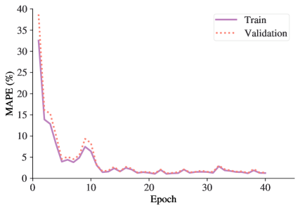
Figure 6: Training progress of the supervised learning NN model during Phase I

(a) Near-optimal vs Predicted Costs

(b) Prediction error for different problem sizes

Figure 7: Phase I test results of NN trained with random VRP instances where $N\in[50,500]$

Our training process for the NN model consists of three phases. In Phase I, the VRP instances were created following the rules of Uchoa et al. (2017) with randomly placed depots and customers, where coordinates are integers from a grid of size $[0,1000]\times[0,1000]$ and demands are integers in the range $[1,100]$. Our large-scale MDVRP Test (T) instances are also generated using the same rules for customer positions, depot positions, and demands. Although this trained model provides good estimates for the initial MDVRP solutions, the prediction error increases significantly in the direction of the optimality as the GA propagates. Phase I training is effective for estimating the cost of random allocation of customers to depots. Figure 7 depicts the training accuracy of this phase with an average mean absolute percentage error (MAPE) of $1.06\%$. However, it fails to incorporate the VRPs due to the near-optimal allocation of customers to depots in the event of an MDVRP decomposition.

In Phase II, CVRP instances were generated from customer allocations from random MDVRP instances to incorporate the near-optimal cases seen during our methodology. $80\%$ of the train data were generated using the two targeted assignment rules, out of which in $70\%$ of the instances, exceptions were made to the targeted assignments by randomly reallocating up to $10\%$ of the customers. A random allocation of customers to depots was used to obtain the remaining $20\%$ of data. In this Phase, we train the NN model using the targeted train data based on a partial understanding of our real data distribution. As a result of comparing multiple assignments, MDVRP solutions are better represented, and cost prediction errors are fewer towards optimal decompositions.

In the final training phase, i.e., Phase III, we generated train/validation data in four steps using random MDVRP instances in conjunction with GANCP. In the first step, the NN prediction model is initialized with randomized parameters $\theta$. For an input CVRP, this untrained model is incapable of a fair cost prediction and would provide a real number as the output based on $\theta$. Therefore, the final solutions from GANCP are random assignments. The obtained VRP subproblems are evaluated and trained with the NN model to update the parameter values. Now, the updated NN model is used in GANCP for random MDVRP instances to generate new VRP decompositions. This process of NN parameter estimation using partial train data is repeated until the generated data from the fourth step is used for NN model training. For each MDVRP evaluation, the top $2$ solutions using GANCP are selected to produce the corresponding CVRP subproblems. Each step contributes to the generation of $1/4$-th of the total train/validation data. Once the data is generated, the HGS-CVRP solver is used to find the near-optimal cost labels with a time limit of $5$ seconds for a CVRP. At each step, the data generated is used for training in combination with data from previous steps, when applicable. This improves the NN model’s ability to evaluate CVRP instances of various assignment patterns observed during our heuristic algorithm.

7.2 T instances

For evaluation of our $\text{GANCP}^{+}$ methodology, $150$ T instances are generated in the range $N\in[100,1500]$ and $D\in[2,10]$. The number of depots for each problem is chosen so that the approximate CVRP subproblem size falls within the range of trained data, i.e., $\frac{N}{D}\in[50,500]$. Instances are generated based on random customer and depot positioning in a grid of size $[0,1000]\times[0,1000]$, while demands are integers in the range of $[1,100]$. T instances were evaluated using each of the above-trained models, and results from an average of 10 experiments and the best out of 10 experiments are reported. Table 1 summarizes the results on T instances for different training phases and compares the results for a test of $1000$ CVRP instances with random customer positions. CVRP optimality gaps are calculated as absolute values for the NN model to avoid overshooting and undershooting. Note that the computational times are recorded in seconds throughout the document.

Table 1: NN model accuracy for different training phases

Train Data Type	CVRP Test Gap	T Ins Gap A	T Ins Gap B
	(%)	(%)	(%)
Phase I	1.06	0.50	-0.49
Phase II	2.21	-0.09	-0.47
Phase III	2.26	-0.58	-0.89

Algorithm Settings

The computational requirements of the HGS-CVRP solver increase as the size of the problem increases. The time limits for the HGS-CVRP solver, shown in Table 2, are used to ensure an equivalent exploration of the solution space for different problem sizes. Additionally, the number of CVRP instances that can be processed by the NN model in a batch depends on the memory limitations of the computer. On the specified computer, the batch processing is executed in units as specified in Table 2 to avoid memory overflows.

Table 2: Hyperparameters used under the given system specifications

Approximate	NN batch size	HGS time
subproblem size		(sec)
$N/D\in[50,100)$	512	0.1
$N/D\in[100,200)$	256	1.0
$N/D\in[200,300)$	128	2.0
$N/D\in[300,400)$	64	2.0
$N/D\in[400,500]$	32	2.0

Benchmark Algorithm

Table 3 shows the performance of our method on benchmark instances in Cordeau et al. (1997). Only instances without route-duration constraints were used in the experiment. We compare our results to the best-known solution costs in the literature. A distinct training of the NN model using random VRP instances of small problem sizes in the range $N\in[10,50]$ was performed to evaluate the subproblems of benchmark instances. Customer and depot positioning were randomly chosen, similar to Phase I train data. As expected, $\text{GANCP}^{+}$ performs relatively poorly for the out-of-distribution Cordeau et al. (1997) instances, with a maximum gap of $4.61\%$. MDVRP’s best-known results are also compared with an open-source VROOM (Coupey et al., 2023) solver on the same machine running Ubuntu 22.04.1, and the results indicate that VROOM is a competitive solver for MDVRP instances that yields high-quality solutions in a short time frame. To ensure that the comparison between the benchmark MDVRP solver and the use of our NN model on a GPU is fair, we run VROOM using 16 CPU threads on the same machine for all future experiments. Through the use of multiple CPU threads, we improve the benchmark solver’s computational speed.

Table 3: Evaluation of Cordeau Instances

		GANCP		$\text{GANCP}^{+}$			VROOM
Instance	Best	NN Cost	Time	Cost	Time	Gap	Cost	Time	Gap
	Known		(sec)		(sec)	(%)		(sec)	(%)
p01-n50-d4	576.87	697.00	1.64	586.39	3.64	1.65	576.87	0.15	0.00
p02-n50-d4	473.53	593.56	1.61	495.38	3.61	4.61	476.66	0.08	0.66
p03-n75-d5	641.19	844.65	2.23	662.14	4.73	3.27	647.89	0.28	1.04
p04-n100-d2	1001.04	1121.68	1.16	1013.37	2.16	1.23	1013.50	0.52	1.24
p05-n100-d2	750.03	876.46	1.24	763.90	2.24	1.85	759.05	0.52	1.20
p06-n100-d3	876.50	1026.63	1.60	885.92	3.11	1.07	884.67	0.55	0.93
p07-n100-d4	881.97	1102.56	1.24	916.65	3.24	3.93	901.82	0.48	2.25

We executed $\text{GANCP}^{+}$ on $150$ MDVRP T instances of varying size, and a summary of the results is shown in Table 4. The results indicate the effectiveness of our approach in obtaining high-quality solutions at faster computational speeds. The appendix contains detailed results of the experiments. VROOM timed is the execution of VROOM with a time limit equal to the run time of $\text{GANCP}^{+}$ heuristic corresponding to the best solution achieved. VROOM, with a shorter time limit, often obtains the same solutions as the full run but fails to improve the early-on solutions. In many real-life applications, the geographical location of customers and demand distributions follow a historical pattern. Thus, NN can be advantageous in training routing problem predictions and solving hierarchical optimization problems in real time.

Table 4: Summary of experiments on T instances

# Nodes	Average of 10 runs			Best	VROOM		Gap A	Gap B
	NN Cost	Cost	Time	Cost	Cost	Time	(%)	(%)
[100,200]	29117.09	29506.57	2.90	29321.03	29498.94	1.66	0.03	-0.60
[201,300]	40341.34	40806.03	7.15	40651.23	41080.90	4.58	-0.67	-1.05
[301,400]	48376.34	48604.29	11.24	48434.45	48987.85	9.85	-0.78	-1.13
[401,500]	57233.29	57929.15	15.42	57719.28	58326.76	22.28	-0.68	-1.04
[501,600]	73598.78	74174.46	22.86	73934.97	74497.23	48.52	-0.43	-0.75
[601,700]	78006.76	78170.21	30.29	77930.80	78687.05	102.69	-0.66	-0.96
[701,800]	99638.54	100795.98	41.97	100516.96	101334.56	155.25	-0.53	-0.81
[801,900]	100531.98	100784.26	45.56	100544.05	101510.61	228.24	-0.72	-0.95
[901,1000]	116908.49	117343.41	54.00	117118.12	118042.43	330.17	-0.59	-0.78
[1001,1100]	124396.17	125074.06	67.32	124800.93	125837.19	453.42	-0.61	-0.82
[1101,1200]	122553.92	123121.97	73.37	122851.90	124239.53	551.04	-0.90	-1.12
[1201,1300]	140751.63	140683.88	82.05	140339.98	141516.74	752.71	-0.59	-0.83
[1301,1400]	156527.15	155526.77	87.82	155101.03	155932.46	923.81	-0.26	-0.53
[1401,1500]	166412.10	166956.54	97.05	166641.89	167286.25	1110.83	-0.20	-0.39

7.3 Out-of-range data

We further evaluate the predictive accuracy of our heuristics for MDVRP instances with approximate subproblem sizes that are outside the range of the trained data. A summary of the results of 50 randomly generated Out-of-range (O) Instances with $\frac{N}{D}\notin[50,500]$ is provided in Table 5. From the results, it can be seen that our method achieves better results than VROOM for problems with $N\in[101,250]$. This is likely because the NN model observes some out-of-range VRP instances during the stepwise training procedure and learns from them. However, our method fails to outperform VROOM for relatively smaller and larger problems in the O instances dataset.

Table 5: Summary of experiments on O instances

# Nodes	Average of 10 runs			Best	VROOM		Gap A	Gap B
	NN Cost	Cost	Time	Cost	Cost	Time	(%)	(%)
[50,100]	16328.06	16513.03	2.15	16467.98	16371.24	0.23	0.94	0.66
[101,150]	22021.44	22027.67	3.65	21930.31	22040.55	0.80	-0.05	-0.49
[151,200]	24994.17	25268.67	4.92	25108.81	25161.54	1.74	0.48	-0.18
[201,250]	35150.75	35246.59	6.55	34999.57	35356.99	4.21	-0.33	-1.03
[1000,1500]	220043.57	223942.65	56.88	223747.96	222183.17	330.73	0.77	0.68

7.4 Out-of-distribution data

The robustness of our heuristic in association with the NN model is tested for multiple combinations of coordinates and demand distributions. Uchoa et al. (2017) uses similar customer positioning and demand distributions to generate a class of VRP benchmark instances.

The positioning of customers is determined using three different rules, namely Random (R), Clustered (C), and Random-Clustered (RC), as described in Solomon (1987) VRPTW instances. In C, a few randomly positioned customers $s\in\text{UD}[3,8]$ act as cluster seeds to attract $N\setminus s$ customers with an exponential decay. In RC, half of the customers are randomly positioned, and the remaining are clustered as in C. Two different types of demand distributions such as Unitary (U), where each demand is equal to 1, and Quadrant-Dependent (Q), where demand belongs to $\text{UD}[1,50]$ for even quadrant and $\text{UD}[51,100]$ for odd quadrant customers, respectively, are considered for evaluation. Our T instances were generated using R customer positioning within the grid and demand from $\text{UD}[1,100]$. Depots are assumed to take a random position on the grid in all cases. Using the above rules, eight classes of out-of-distribution MDVRP instances are generated, as shown in Table 6.

Table 6: D instances generated using multiple combinations of rules

Instance Class	Customer Positioning	Demand Distribution
D1	C	UD[1,100]
D2	RC	UD[1,100]
D3	R	U
D4	R	Q
D5	C	U
D6	C	Q
D7	RC	U
D8	RC	Q

Table 7: Summary of experiments on D instances

Instances	Average of 10 runs			Best	VROOM		Gap A	Gap B
	NN Cost	Cost	Time	Cost	Cost	Time	(%)	(%)
D1	79405.89	77606.12	39.69	77347.84	77202.13	389.16	0.62	0.20
D2	79777.80	80365.79	29.34	80178.28	80189.65	173.94	0.08	-0.19
D3	86458.29	83043.41	35.46	82900.18	82998.27	235.70	0.06	-0.15
D4	85711.91	85326.44	40.43	85002.43	85577.51	288.23	-0.26	-0.69
D5	59134.12	55126.99	22.23	54847.38	54606.09	106.43	1.28	0.56
D6	67575.29	64184.02	37.20	63903.97	63872.70	330.80	0.49	0.06
D7	81024.07	77722.09	26.95	77527.93	77442.77	98.38	0.49	0.23
D8	68419.02	68330.90	22.05	68060.73	67933.00	126.03	0.80	0.17

A performance summary of $\text{GANCP}^{+}$ for eight instance classes, each of different distributions, can be found in Table 7. Given that our NN model was trained over a specific distribution of CVRPs, the results for out-of-distribution instances, while there is a positive optimality gap compared to the solver in some cases, are satisfactory. A noticeable difference is observed for D4 instances, where customer positioning and demand distribution resemble our T instances with minor modifications. The average result of our heuristics in 10 runs for D4 is better than VROOM. Similarly, the maximum deviation from optimality is visible for instances in class D5 where customer locations are purely clustered, and all demands are assumed to be unitary. Moreover, we still retain a considerable computational advantage for out-of-distribution data as well as being able to achieve satisfactory results.

8 Computational Study for CLRP

Our modified genetic algorithm for CLRP is carried out by using the same set of trained parameters $\theta$ as in the MDVRP experiments. Note that some local searches, such as random mutations, are not considered in this evaluation of CLRP benchmark datasets. We focus on our main goal in the applicability of decomposition evaluation using cost prediction and thus do not explore additional solution improvement strategies for CLRP. We analyze the performance of our modified heuristic in two popular CLRP benchmark sets, Tuzun and Burke (1999) and Barreto (2004). Tuzun and Burke (1999) contains $36$ instances with $N\in\{100,150,200\}$ customers, $M\in\{10,20\}$ uncapacitated depots and capacitated vehicles. Customers are distributed in varying densities, and clusters are sized differently in these instances. Barreto (2004) instances are derived from the CVRP instances with up to $150$ customers and $10$ depots. Routing (vehicle) opening costs are ignored in these instances.

Table 8: Evaluation of Barreto benchmark set

Instance	Best	TBSA	$\text{GANCP}^{+}$				Gap
	Known		Best Cost	Time	Opened
					Depots	Vehicles	(%)
Christofides69-50x5	565.6	565.6	592.9	2.90	1	5	4.83
Christofides69-75x10	844.4	848.9	855.8	3.41	2	9	1.35
Christofides69-100x10	833.4	833.4	839.7	3.13	2	8	0.76
Daskin95-88x8	355.8	355.8	355.8	3.18	2	8	0.00
Daskin95-150x10	43919.9	43919.9	47303.6	7.35	4	14	7.70
Gaskell67-21x5	424.9	424.9	429.6	3.37	2	5	1.11
Gaskell67-22x5	585.1	585.1	585.1	3.01	1	3	0.00
Gaskell67-29x5	512.1	512.1	512.1	2.57	2	4	0.00
Gaskell67-32x5-1	562.2	562.2	562.2	3.02	1	4	0.00
Gaskell67-32x5-2	504.3	504.3	504.3	2.70	1	3	0.00
Gaskell67-36x5	460.4	460.4	460.4	2.54	1	4	0.00
Min92-27x5	3062.0	3062.0	3062.0	2.85	2	4	0.00
Min92-134x8	5709.0	5709.0	6112.0	4.95	4	11	7.06
						Average	1.75

Table 9: Evaluation of Tuzun-Burke benchmark set

Instance	Best	TBSA	$\text{GANCP}^{+}$				Gap
	Known		Best Cost	Time	Opened
					Depots	Vehicles	(%)
111112	1467.68	1467.68	1500.42	3.35	2	11	2.23
111122	1448.37	1448.37	1453.89	2.99	2	11	0.38
111212	1394.80	1394.80	1427.53	4.01	2	11	2.35
111222	1432.29	1432.29	1435.36	3.97	2	11	0.21
112112	1167.16	1167.16	1217.84	3.35	2	12	4.34
112122	1102.24	1102.24	1102.24	3.50	2	10	0.00
112212	791.66	791.66	791.66	3.21	2	11	0.00
112222	728.30	728.30	728.30	3.15	2	11	0.00
113112	1238.24	1238.24	1285.25	3.30	2	11	3.80
113122	1245.30	1245.30	1255.51	3.32	2	11	0.82
113212	902.26	902.26	902.26	3.28	3	12	0.00
113222	1018.29	1018.29	1051.20	3.62	3	11	3.23
121112	2237.73	2237.73	2307.14	3.34	3	22	3.10
121122	2137.45	2137.45	2264.78	4.87	3	22	5.96
121212	2195.17	2195.17	2257.68	3.69	3	22	2.85
121222	2214.86	2214.86	2276.02	3.77	4	22	2.76
122112	2070.43	2070.43	2096.32	3.25	2	21	1.25
122122	1685.52	1685.52	1712.32	4.34	3	21	1.59
122212	1449.93	1449.93	1469.70	3.08	2	20	1.36
122222	1082.46	1082.46	1160.78	3.51	3	22	7.24
123112	1942.23	1942.23	1974.40	4.36	4	22	1.66
123122	1910.08	1910.08	2102.32	4.58	4	22	10.06
123212	1760.84	1761.11	1778.96	3.33	2	22	1.03
123222	1390.86	1390.86	1423.86	4.93	5	22	2.37
131112	1866.75	1892.17	1944.22	3.42	2	15	4.15
131122	1819.68	1819.68	1880.57	4.64	3	16	3.35
131212	1960.02	1960.02	2038.57	3.18	3	17	4.01
131222	1792.77	1792.77	1879.86	3.45	2	16	4.86
132112	1443.32	1443.32	1531.33	3.90	3	16	6.10
132122	1429.30	1429.30	1446.68	3.54	2	16	1.22
132212	1204.42	1204.42	1204.42	3.01	3	17	0.00
132222	924.68	924.68	998.24	3.05	2	17	7.96
133112	1694.18	1694.18	1757.34	3.97	2	16	3.73
133122	1392.00	1392.01	1408.83	4.01	4	16	1.21
133212	1197.95	1197.95	1217.50	3.08	3	17	1.63
133222	1151.37	1151.37	1214.22	3.99	4	17	5.46
						Average	2.84

CLRP’s best-known solutions (BKS) have been compiled from the literature, which is widely spread in multiple research studies. We also compare our $\text{GANCP}^{+}$ performance with TBSA, as it is one of the most effective heuristics for CLRP. In a few instances, $\text{GANCP}^{+}$ achieves proven optimal solutions. Tables 8 and 9 show that our NN model provides good estimates of the decompositions leading to good solutions, even when the prediction model has been trained on a different distribution of CVRPs.

9 Conclusions

In this work, we propose a genetic algorithm to solve the MDVRP based on a decomposition approach where the fitness of a chromosome is evaluated using a neural network-based cost predictor instead of solving the optimization subproblem. Our method GANCP in conjunction with a hybrid genetic algorithm for post-processing is referred to as $\text{GANCP}^{+}$. Numerical experiments show that our approach is effective in obtaining good solutions for large-scale data with significant computational advantages in comparison to an effective open-source MDVRP solver VROOM. The accuracy of the prediction model depends on the similarity of training and testing data distributions and problem size. Our experiments on out-of-distribution and out-of-range instances show that the results are satisfactory for practical execution with a significant advantage in computational time. A direct extension of this work is to consider route duration constraints for the MDVRP. The idea of subproblem cost prediction is a promising research direction and can be applied to multiple optimization problems such as Periodic VRP, VRP with profits, VRP with time windows, Split Delivery VRP, etc. We verify this idea by using the existing trained NN model to evaluate the Capacitated Location Routing Problem benchmark datasets. It further validates the transferability of the trained model for a more generalized problem and still leads to satisfactory results.

Detailed Results of Computational Experiments

Table 10: Results of T instances

Instance	Average of 10 runs				Best of 10 runs				VROOM		VROOM timed		Gap A	Gap B
	NN Cost	Time	$\text{GANCP}^{+}$	Time	NN Cost	Time	$\text{GANCP}^{+}$	Time	Cost	Time	Cost	Time	(%)	(%)
T001-n100-d2	16553.16	1.01	17315.14	2.01	16572.26	0.95	17183.24	1.95	17166.17	0.50	17166.17	0.49	0.87	0.10
T002-n113-d2	22450.15	1.04	22554.59	2.02	22349.68	1.04	22500.46	2.04	22489.61	0.78	22489.61	0.78	0.29	0.05
T003-n127-d2	24704.28	1.18	25462.76	2.18	24580.86	1.18	25138.36	2.18	25330.31	0.86	25330.31	0.83	0.52	-0.76
T004-n143-d2	34057.09	1.32	35250.60	2.32	34240.41	1.28	35023.34	2.28	35259.19	1.06	35259.19	1.13	-0.02	-0.67
T005-n151-d3	23013.48	1.68	24175.28	3.18	23013.48	1.67	24175.28	3.17	24081.61	1.18	24081.61	1.18	0.39	0.39
T006-n167-d2	32767.70	1.49	33020.89	2.49	32797.49	1.46	32764.11	2.47	32671.05	1.88	32671.05	1.84	1.07	0.28
T007-n196-d3	28533.28	2.13	27711.31	3.63	28241.50	2.11	27557.16	3.61	27893.84	2.18	27893.84	2.17	-0.65	-1.21
T008-n198-d2	41817.22	1.70	41229.69	2.70	41649.54	1.68	40981.93	2.68	41398.74	3.05	41398.74	2.78	-0.41	-1.01
T009-n199-d3	35547.01	2.14	36965.70	3.64	35864.57	2.19	36783.30	3.69	36923.56	2.39	36923.56	2.42	0.11	-0.38
T010-n200-d4	31727.54	2.80	31379.72	4.80	31610.42	2.89	31103.13	4.89	31775.31	2.74	31775.31	2.71	-1.24	-2.12
T011-n203-d3	34627.33	2.31	34382.04	3.81	34846.36	2.32	34278.09	3.82	34305.96	2.72	34305.96	2.67	0.22	-0.08
T012-n207-d4	30453.94	2.80	31588.49	4.80	29970.32	2.80	31369.87	4.80	32042.14	3.37	32042.14	3.34	-1.42	-2.10
T013-n222-d3	42589.75	2.56	43565.26	4.06	42582.72	2.62	43125.71	4.12	43287.22	3.06	43287.22	3.02	0.64	-0.37
T014-n229-d2	38898.84	2.20	38405.54	12.20	37913.70	2.18	38320.44	12.18	38721.88	3.61	38721.88	3.57	-0.82	-1.04
T015-n232-d4	40301.62	3.39	40525.98	5.39	40128.80	3.42	40361.03	5.43	40492.83	3.52	40492.83	3.50	0.08	-0.33
T016-n235-d3	39610.28	2.69	41510.99	4.19	39627.43	2.72	41470.60	4.22	42086.26	3.60	42086.26	3.67	-1.37	-1.46
T017-n269-d5	33460.22	4.45	34119.98	6.95	33470.84	4.43	33904.89	6.93	34389.10	3.85	34389.10	3.88	-0.78	-1.41
T018-n276-d2	49908.66	2.78	49289.98	12.78	49974.84	2.85	49264.31	12.85	50123.49	5.27	50123.49	5.44	-1.66	-1.71
T019-n288-d4	35480.95	4.34	35718.69	6.34	35323.99	4.42	35594.19	6.42	35927.17	5.68	35927.17	5.80	-0.58	-0.93
T020-n297-d2	50630.73	3.06	50661.79	13.06	50338.92	2.95	50606.84	12.96	51370.55	6.21	51370.55	6.39	-1.38	-1.49
T021-n298-d3	47792.38	3.55	49097.61	5.05	47809.72	3.53	48867.59	5.03	49143.33	9.51	49143.33	5.36	-0.09	-0.56
T022-n306-d3	47299.71	3.83	48104.63	18.83	47423.41	3.76	48050.86	18.76	49115.12	6.03	49115.12	6.20	-2.06	-2.17
T023-n308-d5	37624.79	5.20	38724.29	7.70	37770.39	5.10	38610.51	7.60	38860.82	7.80	38860.82	7.74	-0.35	-0.64
T024-n314-d5	40865.76	5.25	40846.95	7.75	41054.88	5.19	40488.90	7.69	41139.55	10.47	41139.55	8.14	-0.71	-1.58
T025-n314-d6	36171.00	5.87	36555.12	8.87	36624.60	5.90	36399.74	8.90	36660.97	7.98	36660.97	8.23	-0.29	-0.71
T026-n324-d5	43090.65	5.54	43958.06	8.05	43306.11	5.64	43407.38	8.14	43423.42	6.67	43423.42	6.29	1.23	-0.04
T027-n326-d2	55351.76	3.41	54587.47	13.42	55136.66	3.29	54387.16	13.30	54856.20	7.83	54856.20	8.03	-0.49	-0.86
T028-n339-d4	47322.44	4.95	47783.97	6.96	47369.11	5.09	47691.77	7.09	47938.52	8.84	47938.52	7.43	-0.32	-0.51
T029-n348-d3	65707.48	4.59	65270.16	19.60	65436.03	4.49	65202.67	19.49	66172.13	10.76	66172.13	11.14	-1.36	-1.47
T030-n355-d6	50930.74	6.86	51699.52	9.87	50191.62	6.69	51414.50	9.69	51907.11	10.51	51907.11	9.89	-0.40	-0.95
T031-n359-d7	43514.97	7.52	42584.23	11.02	43677.50	7.34	42536.33	10.84	42970.07	11.56	42970.07	11.06	-0.90	-1.01
T032-n367-d5	41662.81	6.44	42003.96	8.94	41620.55	6.35	41787.08	8.85	42287.09	10.99	42287.09	9.30	-0.67	-1.18
T033-n380-d2	69376.44	4.20	69304.32	14.21	69338.15	4.17	69300.57	14.18	70364.10	12.69	70364.10	13.06	-1.51	-1.51
T034-n393-d6	49973.83	7.96	50433.09	10.96	49990.52	8.06	50370.40	11.06	51146.93	15.88	51146.93	12.33	-1.40	-1.52
T035-n402-d6	47911.93	8.04	49138.92	11.04	47691.78	8.30	48942.76	11.30	49288.75	17.79	49288.75	12.11	-0.30	-0.70
T036-n405-d3	73434.15	5.54	74281.41	20.55	74293.45	5.71	74023.18	20.71	74816.30	15.67	74816.30	16.79	-0.71	-1.06
T037-n409-d5	65174.49	7.37	67507.97	9.87	65209.96	7.37	67458.47	9.88	67186.06	17.31	67186.06	10.59	0.48	0.41
T038-n411-d8	38738.91	10.03	39926.70	14.03	39154.52	9.96	39775.92	13.96	40227.96	12.75	40227.96	12.81	-0.75	-1.12
T039-n426-d5	52346.05	7.89	54223.79	10.39	52685.60	7.71	54014.84	10.21	54699.31	28.62	54949.84	11.25	-0.87	-1.25
T040-n426-d3	58263.56	5.88	57771.13	20.88	58121.93	5.98	57732.58	20.99	59195.59	23.61	59195.59	21.96	-2.41	-2.47
T041-n429-d7	43703.81	9.67	43703.07	13.17	43807.12	9.43	43638.52	12.93	44248.05	15.94	44248.05	13.48	-1.23	-1.38
T042-n442-d5	58721.94	8.22	58947.15	10.73	59348.71	8.17	58374.75	10.67	58666.22	19.78	58666.22	11.31	0.48	-0.50
T043-n465-d2	84669.22	5.56	85760.01	25.57	84549.69	5.72	85587.25	25.72	86902.96	29.52	86902.96	26.90	-1.32	-1.51
T044-n482-d8	49984.72	12.53	49725.66	16.53	49826.80	13.11	49338.53	17.11	49903.86	31.06	49903.86	18.51	-0.36	-1.13
T045-n489-d7	61848.66	11.18	61895.05	14.68	61930.31	10.91	61649.19	14.42	62185.92	29.83	62185.92	15.56	-0.47	-0.86
T046-n497-d9	52002.07	13.06	52268.90	17.56	52295.85	12.87	52095.42	17.37	52600.17	25.49	52600.17	19.27	-0.63	-0.96
T047-n503-d3	78054.59	7.19	79218.41	22.20	77829.63	7.27	79084.49	22.28	79547.74	56.52	79547.74	24.38	-0.41	-0.58
T048-n505-d6	61682.04	10.54	61846.28	13.55	61668.49	10.43	61539.96	13.43	61555.26	36.23	61599.50	14.67	0.47	-0.02
T049-n509-d8	51403.11	12.65	50581.33	16.65	51686.86	12.82	50278.10	16.82	50857.82	39.48	50857.82	19.36	-0.54	-1.14
T050-n510-d2	91931.96	6.21	93549.19	26.22	91859.63	6.40	93415.66	26.42	94044.04	35.12	94044.04	27.68	-0.53	-0.67
T051-n524-d9	56690.04	14.22	56451.31	18.73	57178.70	14.33	56169.36	18.83	56508.63	32.84	56508.63	21.47	-0.10	-0.60
T052-n527-d2	100910.17	6.54	102462.67	26.55	100449.18	6.48	102302.44	26.49	103008.16	36.05	103008.16	28.16	-0.53	-0.69
T053-n534-d10	55644.95	15.56	56424.74	20.56	55402.19	15.71	56179.64	20.71	56749.52	30.71	56749.52	22.91	-0.57	-1.00
T054-n540-d7	79479.85	12.66	80678.59	16.17	79274.33	12.74	80241.18	16.25	80059.69	58.48	80059.69	17.80	0.77	0.23
T055-n566-d5	80285.61	10.89	80317.27	35.89	80071.35	10.94	80053.77	35.95	80780.27	49.44	80780.27	38.63	-0.57	-0.90
T056-n568-d4	84066.56	9.76	82199.30	29.77	84178.61	9.99	82164.22	30.00	83556.16	55.14	83556.16	33.19	-1.62	-1.67
T057-n575-d8	58550.50	14.56	58945.34	18.57	58300.47	14.54	58411.12	18.54	58955.89	42.22	58955.89	20.66	-0.02	-0.92
T058-n579-d2	98187.65	7.63	100464.83	27.65	98160.17	7.81	100341.27	27.83	100663.45	95.22	100663.45	31.91	-0.20	-0.32
T059-n581-d7	58646.00	13.69	59597.09	17.19	58638.11	13.81	59343.40	17.32	59614.05	60.39	59878.72	18.89	-0.03	-0.45
T060-n593-d4	74849.83	10.39	75706.15	30.40	74885.91	10.38	75564.90	30.38	77060.51	51.47	77060.51	34.24	-1.76	-1.94
T061-n603-d6	67309.91	13.34	66127.94	43.34	67309.91	13.24	66127.94	43.25	67270.27	76.83	67270.27	48.01	-1.70	-1.70
T062-n618-d9	64666.71	17.15	63988.05	21.66	64836.56	17.05	63879.86	21.55	64736.50	98.16	64769.85	24.81	-1.16	-1.32
T063-n623-d2	105633.81	9.04	106273.68	29.07	105823.64	8.94	106161.43	28.96	106461.77	81.29	106461.77	31.60	-0.18	-0.28
T064-n634-d4	84698.75	11.15	85389.24	31.16	84827.26	10.99	85330.18	31.00	86214.91	92.96	86214.91	35.54	-0.96	-1.03
T065-n647-d9	59704.36	18.64	60284.43	23.14	59955.58	18.86	60113.71	23.36	60554.03	99.27	60643.85	27.64	-0.45	-0.73
T066-n680-d5	97205.11	13.94	97929.07	38.95	97752.78	14.03	97429.40	39.04	98220.53	95.60	98220.53	43.40	-0.30	-0.81
T067-n682-d8	64433.33	18.62	66402.29	22.62	64760.69	18.40	66108.98	22.40	66696.34	148.73	67153.71	25.44	-0.44	-0.88
T068-n684-d7	65112.27	17.30	65034.52	20.81	64893.53	17.29	64657.34	20.80	65503.01	100.25	65503.01	24.31	-0.72	-1.29
T069-n686-d4	96952.69	12.91	96006.46	32.92	98751.09	12.88	95345.17	32.89	95966.77	106.22	95966.77	37.81	0.04	-0.65
T070-n692-d5	74350.61	14.27	74266.39	39.27	74185.54	14.22	74153.97	39.22	75246.33	127.60	75246.33	45.19	-1.30	-1.45
T071-n723-d6	83098.01	17.29	83867.82	47.30	83298.31	17.58	83666.89	47.59	84919.30	158.59	84919.30	53.24	-1.24	-1.47
T072-n734-d7	70067.65	18.67	70008.68	53.68	70265.25	18.80	69739.71	53.81	71147.92	122.61	71149.48	60.08	-1.60	-1.98
T073-n745-d3	106860.85	13.63	107700.60	43.66	106775.14	13.71	107371.74	43.73	108173.93	209.11	108173.93	50.41	-0.44	-0.74
T074-n756-d5	89410.22	16.54	89528.35	41.55	88576.01	16.68	89235.37	41.70	90896.57	132.71	90998.02	47.77	-1.51	-1.83
T075-n777-d10	72722.36	25.12	72682.64	30.12	71872.47	25.07	72368.54	30.07	72726.66	155.51	72831.48	35.81	-0.06	-0.49
T076-n789-d2	149084.74	13.12	156080.91	33.15	148717.15	13.28	155770.73	33.30	155606.23	175.99	155606.23	38.07	0.31	0.11
T077-n794-d3	126225.92	14.34	125702.85	44.36	126020.00	14.42	125465.72	44.44	125871.32	132.21	125871.32	49.37	-0.13	-0.32
T078-n803-d4	103011.71	16.33	100427.03	56.35	104121.95	16.41	100085.25	56.43	101208.62	144.27	101208.62	64.10	-0.77	-1.11
T079-n810-d7	81296.17	21.82	80410.27	56.83	81092.54	22.42	80203.44	57.43	81726.09	204.31	81726.09	64.18	-1.61	-1.86
T080-n816-d3	156839.64	15.36	154770.21	45.39	156887.23	15.18	154764.43	45.21	154897.13	179.42	154897.13	51.42	-0.08	-0.09
T081-n817-d6	83751.60	20.21	83325.57	50.22	83974.90	20.02	83069.44	50.03	85041.40	196.15	85041.40	53.87	-2.02	-2.32
T082-n820-d3	99951.16	15.55	101516.00	45.57	100857.08	15.25	101069.89	45.26	102080.29	284.99	102080.29	54.59	-0.55	-0.99
T083-n831-d5	99536.21	19.01	98684.59	44.03	99824.62	18.85	98552.29	43.86	99617.52	182.24	99617.52	49.64	-0.94	-1.07
T084-n858-d6	89026.06	21.33	89889.84	51.34	88822.20	21.61	89675.35	51.61	90993.54	206.43	90993.54	56.78	-1.21	-1.45
T085-n859-d10	69405.42	28.70	69436.16	33.70	69475.73	28.66	69344.10	33.66	70188.38	209.29	70188.38	41.59	-1.07	-1.20
T086-n864-d7	82035.41	24.06	82539.78	59.07	82178.62	24.72	82159.35	59.73	84005.31	264.38	84005.31	68.27	-1.74	-2.20
T087-n867-d9	74842.08	27.90	75544.66	32.40	75360.29	27.26	75364.30	31.77	76007.36	241.15	76007.36	37.82	-0.61	-0.85
T088-n871-d3	142145.70	17.35	142083.23	47.39	141900.85	17.64	141628.80	47.66	142381.34	334.79	142381.34	54.47	-0.21	-0.53
T089-n871-d2	136886.35	16.62	140354.87	36.66	136760.01	16.81	140028.42	36.84	139854.93	242.94	139854.93	45.02	0.36	0.12
T090-n899-d9	88188.19	28.85	91213.19	33.36	88049.00	28.89	91127.65	33.40	91636.03	276.72	91636.03	39.47	-0.46	-0.55
T091-n903-d8	84326.78	27.62	84890.96	67.63	85353.18	27.76	84671.14	67.76	86309.03	320.92	86309.03	78.28	-1.64	-1.90
T092-n905-d4	114491.36	20.06	111349.14	60.08	114801.56	19.65	111193.74	59.66	112733.10	204.08	112733.10	69.45	-1.23	-1.37
T093-n923-d3	129804.53	18.68	131532.07	48.71	130626.41	18.20	131240.89	48.23	132114.76	307.15	132114.76	57.77	-0.44	-0.66
T094-n924-d2	145856.23	18.75	149205.18	38.80	145545.28	18.81	149067.94	38.86	149215.21	423.03	149215.21	46.51	-0.01	-0.10
T095-n935-d6	100996.00	24.73	99495.71	54.74	101593.91	24.22	99103.53	54.23	100293.22	275.39	100293.22	65.68	-0.80	-1.19
T096-n943-d7	123099.97	27.29	120442.95	62.31	122453.18	26.92	120283.93	61.94	121321.95	290.12	121321.95	70.10	-0.72	-0.86
T097-n955-d5	115041.59	23.22	116150.59	48.24	115868.20	23.67	115919.05	48.69	116720.57	459.82	116720.57	60.57	-0.49	-0.69
T098-n972-d10	84943.55	34.17	86073.25	39.18	84641.04	33.55	85681.08	38.57	86493.27	395.53	86493.27	47.37	-0.49	-0.94
T099-n985-d2	183225.95	21.31	187548.18	41.35	183225.95	21.33	187523.11	41.35	186937.02	301.76	186937.02	51.35	0.33	0.31
T100-n1000-d9	87298.92	33.93	86746.11	78.94	87478.59	33.69	86496.79	78.69	88286.12	323.93	88313.91	91.69	-1.74	-2.03
T101-n1012-d3	133386.18	22.05	136702.19	52.11	133908.63	21.89	136314.29	51.92	137128.19	503.12	137128.19	62.88	-0.31	-0.59
T102-n1024-d6	113487.73	28.51	112393.72	58.52	113618.40	28.52	111780.84	58.54	113598.46	315.52	113598.46	66.28	-1.06	-1.60
T103-n1036-d6	117209.51	28.91	118602.35	58.93	116733.89	29.48	118451.87	59.50	119230.85	485.94	119230.85	73.00	-0.53	-0.65
T104-n1039-d10	80207.17	37.32	79751.46	87.33	80322.15	37.45	79493.12	87.45	81504.88	429.35	81504.88	103.47	-2.15	-2.47
T105-n1047-d5	137159.93	27.44	137152.49	77.46	137281.90	27.44	136981.06	77.47	138035.45	433.75	138035.45	91.39	-0.64	-0.76
T106-n1050-d4	135559.82	25.38	135818.12	65.42	135683.24	25.77	135707.54	65.80	136444.69	527.57	136444.69	78.68	-0.46	-0.54
T107-n1069-d6	124901.44	30.40	126846.52	60.42	125241.04	30.44	126564.79	60.46	127508.99	388.72	127508.99	74.26	-0.52	-0.74
T108-n1085-d10	101099.50	40.17	99856.78	90.18	101659.70	39.68	99734.51	89.69	101617.66	488.53	101617.66	107.28	-1.73	-1.85
T109-n1086-d4	130250.51	27.36	133097.33	67.39	129957.41	27.84	132865.80	67.88	133504.62	487.10	133504.62	81.98	-0.31	-0.48
T110-n1094-d3	170699.90	25.38	170519.61	55.42	171287.24	25.96	170115.51	56.00	169798.14	474.56	169798.14	65.97	0.42	0.19
T111-n1109-d10	95929.01	41.56	95231.63	91.56	96211.32	40.47	95014.25	90.48	96864.21	609.60	96864.21	105.37	-1.69	-1.91
T112-n1112-d7	115983.72	34.76	116944.58	69.77	116341.74	35.13	116613.98	70.15	118486.60	372.79	118486.60	84.96	-1.30	-1.58
T113-n1160-d7	116637.40	37.24	117573.47	72.26	116801.56	36.39	117389.65	71.40	119276.20	577.77	119355.61	87.51	-1.43	-1.58
T114-n1178-d3	156795.91	29.60	158060.74	59.64	158290.13	28.56	157542.17	58.61	157700.30	660.99	157700.30	71.18	0.23	-0.10
T115-n1195-d7	127423.57	38.60	127799.41	73.62	127862.09	38.78	127699.43	73.80	128870.34	534.07	128870.34	86.26	-0.83	-0.91
T116-n1209-d9	107538.47	45.51	105386.76	90.52	108132.34	45.76	105084.45	90.78	107213.41	627.89	107213.41	102.73	-1.70	-1.99
T117-n1214-d8	117275.13	42.56	113478.04	82.57	118165.31	43.60	113112.51	83.62	114964.45	642.77	114964.45	100.03	-1.29	-1.61
T118-n1229-d4	192079.47	35.13	194043.87	75.17	191751.01	35.30	193845.81	75.34	194196.06	720.72	194196.06	89.94	-0.08	-0.18
T119-n1235-d9	98876.96	46.84	100185.33	91.85	99173.31	47.36	99717.09	92.37	102023.33	631.84	102041.54	116.60	-1.80	-2.26
T120-n1248-d5	132321.77	37.07	130430.20	87.10	133220.92	36.93	129911.19	86.95	131277.99	551.14	131277.99	107.53	-0.65	-1.04
T121-n1258-d3	175925.98	34.40	178135.55	64.45	177976.30	33.99	177304.83	64.04	177554.29	802.46	177554.29	83.57	0.33	-0.14
T122-n1264-d8	118013.90	45.64	114004.01	85.66	118298.26	44.95	113728.75	84.97	115954.00	795.74	116461.00	101.22	-1.68	-1.92
T123-n1266-d3	207573.56	35.34	213058.09	65.40	207142.97	35.99	212950.25	66.06	211823.19	773.96	211823.19	81.78	0.58	0.53
T124-n1274-d8	119675.00	46.53	120763.31	86.55	119867.91	47.03	120452.11	87.04	121600.10	950.42	121600.10	110.27	-0.69	-0.94
T125-n1282-d9	122120.43	49.45	122656.43	94.47	122334.40	50.37	122454.05	95.39	124118.94	971.50	124118.94	115.83	-1.18	-1.34
T126-n1288-d7	156867.22	43.79	155381.08	78.82	157145.39	43.35	155178.70	78.37	155958.43	811.37	155958.43	103.53	-0.37	-0.50
T127-n1307-d9	116588.78	50.13	114634.46	95.16	117943.23	50.33	114010.67	95.35	116019.74	850.76	116019.74	115.33	-1.19	-1.73
T128-n1313-d7	132072.48	45.17	131515.32	80.19	132295.46	45.37	131308.79	80.40	132031.36	1044.56	132031.36	103.08	-0.39	-0.55
T129-n1316-d9	136132.01	50.90	134836.31	95.92	136835.38	49.94	134379.45	94.95	135909.98	990.16	135909.98	116.71	-0.79	-1.13
T130-n1330-d3	181088.57	38.59	180034.69	68.65	183624.14	38.38	179657.59	68.44	179318.58	975.40	179318.58	89.59	0.40	0.19
T131-n1334-d8	153130.75	48.77	151301.40	88.80	154594.38	48.40	150873.28	88.42	151824.31	711.69	151824.31	105.73	-0.34	-0.63
T132-n1357-d6	156737.67	45.29	158392.38	105.32	157090.76	44.96	157846.18	104.99	158945.23	881.19	158945.23	125.32	-0.35	-0.69
T133-n1367-d3	194203.06	41.52	194883.83	71.57	194964.72	41.69	194577.00	71.73	193117.99	864.75	193117.99	86.08	0.91	0.76
T134-n1369-d7	147384.09	48.67	146367.35	83.70	147752.71	48.24	146037.32	83.26	147257.34	1003.38	147257.34	102.89	-0.60	-0.83
T135-n1377-d8	139862.53	52.21	135927.93	92.24	140619.68	51.98	135310.68	92.00	137546.06	943.86	137546.06	114.75	-1.18	-1.63
T136-n1393-d9	116212.09	55.63	114523.54	100.65	116186.72	55.28	113954.07	100.29	115941.32	816.88	115941.32	120.41	-1.22	-1.71
T137-n1398-d4	248386.57	43.74	248377.29	83.81	249829.27	44.20	248156.34	84.26	247345.20	1079.25	247345.20	109.30	0.42	0.33
T138-n1403-d3	197503.76	45.01	199168.47	75.11	198397.07	45.05	198730.98	75.36	197685.13	897.59	197685.13	89.96	0.75	0.53
T139-n1412-d8	150265.32	54.36	152103.87	94.39	150514.54	54.68	151895.39	94.70	152670.38	824.18	152670.38	113.81	-0.37	-0.51
T140-n1416-d6	144065.03	48.45	143045.96	108.48	145102.85	47.69	142810.76	107.73	143970.64	1091.44	143970.64	130.62	-0.64	-0.81
T141-n1420-d4	215670.00	44.22	218922.90	84.28	215670.00	44.63	218922.74	84.68	218221.47	1026.84	218221.47	105.88	0.32	0.32
T142-n1421-d5	153487.60	47.75	153863.12	97.78	154060.54	47.74	153623.91	97.78	154568.56	1047.29	154568.56	122.43	-0.46	-0.61
T143-n1435-d7	154796.83	52.90	160469.56	122.93	154924.93	53.04	160244.62	123.06	161428.99	1121.70	161428.99	148.12	-0.59	-0.73
T144-n1442-d4	172676.80	46.39	174375.78	86.43	173445.11	45.43	173786.05	85.48	174162.14	984.09	174162.14	101.50	0.12	-0.22
T145-n1444-d6	149798.24	50.71	144344.69	110.74	151345.11	50.37	144083.52	110.41	145903.76	1065.12	145903.76	128.88	-1.07	-1.25
T146-n1455-d5	164432.19	47.88	163710.61	97.91	165592.08	49.39	163484.26	99.42	164500.99	1061.19	164500.99	122.63	-0.48	-0.62
T147-n1480-d10	123792.98	65.23	122356.36	115.25	124349.50	65.11	122006.96	115.14	123704.54	1257.74	123704.54	146.43	-1.09	-1.37
T148-n1486-d4	197865.09	48.17	194736.76	88.23	198642.04	47.70	194516.38	87.76	194583.28	1570.57	194583.28	114.61	0.08	-0.03
T149-n1494-d3	191113.36	48.48	191983.30	78.55	192550.93	48.44	191283.05	78.51	190969.10	1301.99	190973.31	102.45	0.53	0.16
T150-n1500-d5	147890.13	51.51	151353.62	101.55	148648.78	51.62	150955.98	101.66	152352.28	1191.00	152352.28	130.73	-0.66	-0.92
Average													-0.59	-0.90

Table 11: Results of O instances

Instance	Average of 10 runs				Best of 10 runs				VROOM		Gap A	Gap B
	NN Cost	Time	$\text{GANCP}^{+}$	Time	NN Cost	Time	$\text{GANCP}^{+}$	Time	Cost	Time	(%)	(%)
O01-n55-d2	13120.58	0.86	13119.74	1.87	13120.58	2.00	13119.74	3.02	13046.00	0.11	0.57	0.57
O02-n58-d2	13795.52	0.71	13484.07	1.70	13795.52	0.70	13484.07	1.70	13396.68	0.11	0.65	0.65
O03-n64-d2	18300.79	0.81	17721.86	1.82	18147.48	0.82	17719.46	1.82	17634.26	0.14	0.50	0.48
O04-n70-d2	15780.17	0.78	16344.11	1.78	15727.08	0.78	16287.42	1.78	16284.54	0.14	0.37	0.02
O05-n72-d2	17405.01	0.79	17764.05	1.79	17405.01	0.77	17764.05	1.77	17668.66	0.18	0.54	0.54
O06-n74-d2	16809.40	0.80	16888.19	1.81	17042.84	0.84	16835.85	1.84	16798.60	0.20	0.53	0.22
O07-n75-d3	15702.28	1.04	15327.23	2.55	15745.88	1.08	15323.38	2.58	15020.76	0.27	2.04	2.01
O08-n78-d2	15138.23	0.79	15306.72	1.79	15212.67	0.77	15108.62	1.77	15062.94	0.18	1.62	0.30
O09-n84-d3	15286.93	1.19	16523.24	2.69	14952.71	1.20	16429.19	2.70	15709.18	0.30	5.18	4.58
O10-n86-d2	19431.91	0.92	19869.00	1.94	19431.91	0.96	19869.00	1.98	20149.83	0.25	-1.39	-1.39
O11-n91-d3	15716.74	1.19	16072.47	2.66	15630.49	1.15	15967.37	2.65	16141.22	0.36	-0.43	-1.08
O12-n96-d2	18101.00	0.92	18632.94	1.92	18209.62	0.91	18587.77	1.91	18838.04	0.33	-1.09	-1.33
O13-n100-d4	17676.24	1.63	17615.75	3.64	18072.63	1.69	17587.82	3.69	17075.42	0.44	3.16	3.00
O14-n104-d4	17913.12	1.66	17019.30	3.66	17969.85	1.68	16971.73	3.68	16872.50	0.45	0.87	0.59
O15-n108-d3	20167.59	1.38	19924.81	2.88	20192.75	1.32	19804.07	2.82	19933.67	0.47	-0.04	-0.65
O16-n116-d4	20765.39	1.67	19583.03	3.67	20742.90	1.65	19501.74	3.65	19602.32	0.62	-0.10	-0.51
O17-n120-d3	18497.58	1.52	18603.24	3.02	18519.01	1.57	18590.85	3.07	18541.54	0.57	0.33	0.27
O18-n124-d4	19908.36	1.87	20424.76	3.87	20094.64	1.85	20342.63	3.85	20533.69	0.80	-0.53	-0.93
O19-n126-d3	21504.54	1.54	21953.41	3.04	21490.86	1.51	21798.10	3.01	21866.33	0.68	0.40	-0.31
O20-n130-d5	22075.37	2.25	20699.88	4.75	22029.50	2.25	20562.09	4.75	20626.56	0.94	0.36	-0.31
O21-n135-d3	21711.80	1.56	22000.31	3.06	21472.18	1.54	21766.66	3.04	22076.84	0.72	-0.35	-1.41
O22-n136-d4	18775.31	1.91	19441.89	3.91	18777.62	1.83	19376.81	3.83	19619.87	0.86	-0.91	-1.24
O23-n141-d3	26770.58	1.72	26739.24	3.22	26578.64	1.69	26621.22	3.19	26515.67	1.01	0.84	0.40
O24-n144-d3	24865.40	1.75	25117.44	3.25	24781.35	1.73	25033.45	3.23	25254.53	0.96	-0.54	-0.88
O25-n145-d5	24456.78	2.48	24405.61	4.99	24643.78	2.46	24361.35	4.98	24631.29	1.14	-0.92	-1.10
O26-n148-d4	28866.93	2.16	30446.77	4.16	29058.94	2.08	30363.39	4.08	30452.34	1.19	-0.02	-0.29
O27-n152-d4	23909.02	2.12	23190.83	4.12	24056.06	2.15	23012.42	4.15	23002.27	1.26	0.82	0.04
O28-n155-d5	22400.90	2.54	22763.71	5.04	22196.92	2.47	22531.04	4.97	22448.21	1.32	1.41	0.37
O29-n156-d4	22736.68	2.15	22881.73	4.15	22755.60	2.10	22699.61	4.10	22491.65	1.21	1.73	0.92
O30-n160-d5	20805.68	2.76	21369.47	5.26	20979.59	2.80	21146.07	5.30	21172.66	1.48	0.93	-0.13
O31-n168-d4	24409.43	2.36	24474.04	4.36	24418.79	2.44	24470.40	4.44	24661.25	1.34	-0.76	-0.77
O32-n170-d5	22899.82	2.76	22556.04	5.27	23034.71	2.73	22317.75	5.23	22214.60	1.55	1.54	0.46
O33-n172-d4	24233.68	2.40	24406.92	4.40	23942.73	2.39	24341.63	4.39	24362.44	1.48	0.18	-0.09
O34-n180-d4	25247.69	2.63	25349.07	4.63	25160.86	2.70	25254.69	4.70	25596.32	1.58	-0.97	-1.33
O35-n185-d5	29161.16	3.08	29247.41	5.58	29437.03	3.05	28917.75	5.55	28925.29	2.37	1.11	-0.03
O36-n190-d5	26621.62	3.10	27792.71	5.60	26639.15	3.05	27666.90	5.55	27751.61	2.30	0.15	-0.31
O37-n192-d4	29165.67	2.64	30495.66	4.64	29165.67	2.62	30495.66	4.62	30592.23	2.17	-0.32	-0.32
O38-n200-d5	28338.64	3.44	28696.39	5.95	28110.76	3.41	28451.80	5.92	28719.89	2.76	-0.08	-0.93
O39-n235-d5	35817.58	3.86	36125.30	6.37	35542.19	3.81	35877.75	6.32	35792.40	3.98	0.93	0.24
O40-n245-d5	34483.92	4.22	34367.88	6.72	34358.67	4.18	34121.39	6.68	34921.58	4.44	-1.59	-2.29
O41-n1050-d2	209828.27	24.20	219915.25	44.25	209003.43	24.13	219880.61	44.15	218719.85	161.32	0.55	0.53
O42-n1159-d2	185472.05	29.24	188159.35	49.28	185535.67	29.47	188034.38	49.50	186810.50	225.55	0.72	0.66
O43-n1173-d2	197200.95	30.84	200890.55	50.88	197214.94	30.42	200407.18	50.43	199873.12	247.61	0.51	0.27
O44-n1225-d2	182652.25	33.34	182235.49	53.38	183394.59	33.09	181895.12	53.14	181660.32	266.65	0.32	0.13
O45-n1249-d2	241640.56	35.01	245262.65	55.10	241108.19	35.42	245090.26	55.52	242165.71	312.11	1.28	1.21
O46-n1318-d2	235774.70	38.29	238350.86	58.32	236098.34	38.81	238220.44	58.85	236007.13	354.64	0.99	0.94
O47-n1330-d2	253226.30	39.17	259360.85	59.22	252670.20	39.20	258961.63	59.26	256601.82	369.99	1.08	0.92
O48-n1364-d2	253759.75	41.31	264193.95	61.35	253422.38	41.11	264086.01	61.13	261990.53	413.47	0.84	0.80
O49-n1402-d2	225343.35	46.29	222983.69	66.38	225343.35	45.79	222983.69	65.85	221057.67	436.67	0.87	0.87
O50-n1500-d2	215537.51	50.61	218073.88	70.66	215596.35	52.43	217920.27	72.47	216945.08	519.33	0.52	0.45
Average											0.49	0.10

Table 12: Results of D instances

Instance	Average of 10 runs				Best of 10 runs				VROOM		Gap A	Gap B
	NN Cost	Time	$\text{GANCP}^{+}$	Time	NN Cost	Time	$\text{GANCP}^{+}$	Time	Cost	Time	(%)	(%)
D1-n105-d2	13652.76	1.09	14272.19	2.09	13392.72	1.14	14156.04	2.14	13966.79	0.37	2.19	1.35
D1-n237-d3	30495.33	2.76	30905.40	4.27	30195.75	2.76	30667.79	4.26	30436.81	3.28	1.54	0.76
D1-n255-d2	64715.86	2.45	63669.52	12.45	64715.86	2.46	63669.52	12.47	63931.22	3.21	-0.41	-0.41
D1-n350-d4	35034.46	5.23	35814.37	7.23	34863.14	5.28	35728.89	7.29	35926.04	9.40	-0.31	-0.55
D1-n416-d8	49348.75	10.23	45202.43	13.25	49762.01	10.10	45063.58	13.40	44776.34	46.41	0.95	0.64
D1-n517-d5	65921.00	9.72	65612.61	34.72	65597.96	9.99	65168.55	34.99	65750.49	46.38	-0.21	-0.89
D1-n1063-d8	77777.84	35.07	74677.58	75.11	78612.17	35.25	74337.72	75.29	74467.69	941.65	0.28	-0.17
D1-n1288-d3	136794.39	37.30	136001.49	67.35	137565.85	36.99	135412.45	67.04	135040.47	520.17	0.71	0.28
D1-n1333-d3	206426.12	38.60	195036.98	68.77	207239.83	38.32	194840.14	68.60	193723.42	580.32	0.68	0.58
D1-n1453-d6	113892.40	51.66	114868.64	111.70	115401.83	51.35	114433.72	111.41	114002.06	1740.45	0.76	0.38
D2-n225-d4	31095.13	3.20	31880.11	5.20	31150.20	3.28	31776.15	5.28	31800.99	2.91	0.25	-0.08
D2-n289-d2	46363.22	2.98	46493.52	12.99	46178.99	2.96	46358.03	12.97	46880.29	3.87	-0.83	-1.11
D2-n446-d6	50755.17	9.33	50480.35	12.34	50906.04	9.32	50165.78	12.32	50367.79	34.54	0.22	-0.40
D2-n467-d5	54963.91	8.73	55623.93	11.25	54676.11	8.80	55492.69	11.32	55440.76	29.59	0.33	0.09
D2-n469-d9	41104.02	12.50	41361.43	17.01	40891.80	12.49	41269.91	16.99	41824.28	77.51	-1.11	-1.33
D2-n577-d3	113853.28	9.03	115449.78	24.04	113840.34	8.78	115426.24	23.81	114942.42	33.47	0.44	0.42
D2-n598-d9	68665.20	17.02	68490.47	21.53	68430.55	17.08	68341.38	21.61	68269.87	176.12	0.32	0.10
D2-n905-d3	135122.55	20.04	136227.53	50.06	135058.10	19.19	136074.30	49.23	135398.79	162.65	0.61	0.50
D2-n1149-d3	123002.16	28.34	122613.29	58.39	123829.23	28.31	122052.76	58.35	121888.70	350.68	0.59	0.13
D2-n1356-d4	132853.38	40.49	135037.44	80.54	133021.32	39.44	134825.57	79.49	135082.62	868.01	-0.03	-0.19
D3-n154-d3	34852.45	1.68	34185.13	3.19	34852.45	1.65	34185.13	3.15	34138.57	0.85	0.14	0.14
D3-n177-d2	35161.24	1.51	34182.21	2.52	35085.14	1.51	34038.42	2.51	33998.02	1.01	0.54	0.12
D3-n247-d2	37504.73	2.40	35779.37	12.40	37325.24	2.40	35676.03	12.40	35903.84	1.73	-0.35	-0.63
D3-n294-d5	39183.31	5.07	37810.46	7.57	39163.25	4.98	37666.86	7.48	37730.98	5.42	0.21	-0.17
D3-n491-d6	56483.44	10.14	54385.41	13.14	56069.70	10.05	54252.02	13.05	54254.96	42.67	0.24	-0.01
D3-n521-d3	74808.23	8.24	72132.17	23.27	74648.36	8.16	71961.79	23.17	72339.41	15.95	-0.29	-0.52
D3-n1018-d5	125479.87	27.04	121077.33	77.08	125447.17	27.34	120871.55	77.39	121107.62	367.77	-0.03	-0.19
D3-n1085-d7	108608.95	33.61	103098.52	68.63	108683.84	33.86	102974.72	68.87	103426.63	672.55	-0.32	-0.44
D3-n1148-d3	175989.32	28.27	167161.43	58.29	176851.84	28.05	166918.42	58.08	166580.22	316.14	0.35	0.20
D3-n1489-d4	176511.37	48.47	170622.06	88.52	176738.28	48.58	170456.85	88.63	170502.44	932.90	0.07	-0.03
D4-n206-d4	26096.64	2.86	26471.97	4.87	26051.33	2.91	26180.63	4.93	25996.98	2.50	1.83	0.71
D4-n300-d4	37745.89	4.43	37460.16	6.43	37476.12	4.38	37226.41	6.38	37680.82	5.89	-0.59	-1.21
D4-n407-d3	56943.06	5.64	56721.52	20.65	56977.67	5.53	56559.23	20.53	57492.66	10.71	-1.34	-1.62
D4-n518-d6	53465.05	10.60	53791.62	13.61	53561.76	10.33	53671.92	13.33	54065.37	56.61	-0.51	-0.73
D4-n816-d5	86506.00	18.79	85718.78	43.81	86715.06	18.92	85246.81	43.93	86453.35	218.73	-0.85	-1.40
D4-n836-d10	71956.42	28.38	71833.28	33.40	71830.11	27.97	71701.61	32.99	72035.33	572.58	-0.28	-0.46
D4-n937-d4	107324.33	20.81	107980.17	60.83	107982.78	20.95	107536.19	60.97	108823.75	263.31	-0.78	-1.18
D4-n980-d3	141768.74	21.74	141841.62	51.77	141460.04	21.88	141331.46	51.92	141680.00	211.99	0.11	-0.25
D4-n1078-d5	113446.01	28.80	114478.61	78.83	113966.60	28.31	114101.77	78.34	114888.41	538.28	-0.36	-0.68
D4-n1325-d5	161866.91	40.08	156966.62	90.12	162311.84	39.57	156468.23	89.61	156658.45	1001.65	0.20	-0.12
D5-n173-d2	31091.85	1.55	30348.10	2.55	31091.85	1.61	30348.10	2.61	30294.37	1.13	0.18	0.18
D5-n188-d3	30187.07	2.16	29099.04	3.32	30187.07	2.15	29099.04	3.45	28977.50	1.26	0.42	0.42
D5-n327-d4	46645.53	4.98	42675.38	6.98	47008.71	5.05	42232.63	7.05	41956.74	6.85	1.71	0.66
D5-n338-d5	33721.74	5.71	32107.76	7.96	34918.14	5.83	30788.70	8.14	30268.50	7.97	6.08	1.72
D5-n376-d6	41444.97	7.39	40189.35	9.30	41477.41	7.35	40020.94	9.26	39652.81	15.35	1.35	0.93
D5-n451-d4	51159.73	7.26	48535.83	27.27	51497.75	7.40	48424.48	27.40	48405.36	18.44	0.27	0.04
D5-n481-d4	78707.88	8.06	69258.96	28.07	80339.53	8.14	69056.36	28.14	68770.32	26.24	0.71	0.42
D5-n483-d5	62789.31	9.44	57947.16	11.10	63140.45	9.50	57624.69	11.31	56995.74	30.42	1.67	1.10
D5-n774-d7	71715.51	20.31	67433.17	55.33	71753.59	20.42	67396.33	55.45	67316.12	261.44	0.17	0.12
D5-n1318-d4	143877.62	39.36	133675.10	70.41	144482.17	39.52	133482.48	71.58	133423.44	695.19	0.19	0.04
D6-n109-d2	20783.63	1.08	19706.16	2.08	20622.64	0.99	19690.67	1.99	19554.78	0.53	0.77	0.69
D6-n281-d2	46393.95	2.95	44832.92	12.95	46393.95	2.95	44832.92	12.95	45264.51	3.96	-0.95	-0.95
D6-n297-d3	42311.02	3.51	41161.03	5.02	42917.10	3.47	40556.48	4.97	40563.14	5.04	1.47	-0.02
D6-n353-d7	54988.05	7.69	49054.30	9.91	54988.05	7.86	49054.30	9.28	49174.16	21.19	-0.24	-0.24
D6-n505-d8	42191.81	13.20	43221.34	15.46	42300.26	13.02	43167.09	16.02	42845.09	86.89	0.88	0.75
D6-n603-d4	106039.66	11.03	98178.77	31.05	106039.66	10.94	98178.18	30.94	98238.34	64.31	-0.06	-0.06
D6-n827-d8	113206.89	24.04	107848.32	64.06	115317.66	23.93	107424.27	63.96	107572.54	419.15	0.26	-0.14
D6-n894-d8	66027.29	27.12	64006.53	67.14	66402.99	26.76	63608.59	66.79	63464.64	533.24	0.85	0.23
D6-n987-d9	82446.11	32.81	76747.24	73.84	83217.42	32.77	75747.88	73.80	76435.96	877.08	0.41	-0.90
D6-n1396-d5	101364.48	50.45	97083.59	90.52	102358.14	47.85	96779.28	87.93	95613.79	1296.63	1.54	1.22
D7-n100-d2	15801.87	1.04	15618.27	2.05	15694.74	1.08	15564.03	2.08	15463.60	0.25	1.00	0.65
D7-n260-d5	35513.99	4.40	34800.25	6.91	35465.57	4.40	34721.21	6.90	34545.92	3.93	0.74	0.51
D7-n287-d5	44611.06	4.82	44037.15	7.33	44993.42	4.78	44001.48	7.30	43532.64	5.40	1.16	1.08
D7-n386-d2	62147.20	4.33	59020.77	14.34	62147.20	4.28	59020.77	14.28	58990.09	6.18	0.05	0.05
D7-n399-d2	55158.03	4.23	53328.72	14.23	55181.18	4.19	53242.81	14.19	53163.55	6.46	0.31	0.15
D7-n494-d3	69557.11	7.19	66198.80	22.20	69547.35	7.06	66131.57	22.07	66277.93	13.60	-0.12	-0.22
D7-n633-d5	83749.06	12.86	79825.00	37.88	84581.12	12.95	79491.06	37.98	79355.94	88.76	0.59	0.17
D7-n661-d4	103492.99	12.34	100014.76	32.35	103773.03	12.46	99640.68	32.48	99725.00	70.69	0.29	-0.08
D7-n817-d4	102620.72	17.17	97041.95	57.19	104288.37	17.09	96215.17	57.11	96363.84	138.82	0.70	-0.15
D7-n1418-d3	237588.70	45.00	227335.22	75.04	237577.83	44.82	227250.53	74.85	227009.22	649.70	0.14	0.11
D8-n105-d2	17076.87	1.06	19049.21	2.07	17250.87	1.11	18734.74	2.11	18578.74	0.40	2.53	0.84
D8-n167-d3	31806.10	1.88	32873.73	3.38	31981.01	1.89	32357.66	3.39	32308.97	1.29	1.75	0.15
D8-n257-d3	38107.55	2.97	38167.63	4.48	37831.69	2.92	38082.38	4.42	37934.63	3.49	0.61	0.39
D8-n364-d4	48540.66	5.58	48475.39	7.58	48388.79	5.59	48247.72	7.60	48285.40	11.27	0.39	-0.08
D8-n373-d7	44017.55	7.95	44804.36	11.47	43795.82	8.03	44554.37	11.57	44323.28	23.58	1.09	0.52
D8-n593-d7	69376.10	14.10	70043.28	17.60	69376.31	13.80	69859.77	17.31	69517.24	118.01	0.76	0.49
D8-n608-d8	61089.49	15.90	61294.88	19.90	62264.79	15.85	60812.51	19.86	60892.67	161.43	0.66	-0.13
D8-n719-d7	66864.91	18.11	67019.28	53.12	67034.39	18.18	66704.40	53.19	67667.85	219.56	-0.96	-1.42
D8-n903-d6	175076.48	24.02	167180.61	54.06	175076.48	24.19	167180.61	54.22	166240.31	387.51	0.57	0.57
D8-n916-d5	132234.50	21.76	134400.62	46.79	132684.31	21.55	134073.10	46.58	133580.89	333.77	0.61	0.37

Table 13: Detailed results of Tuzun-Burke CLRP Instances

Instance	Best	$\text{TBSA}_{\text{speed}}$		$\text{TBSA}_{\text{qual}}$		$\mkern 1.5mu\overline{\mkern-1.5mu\text{TBSA}\mkern-1.5mu}\mkern 1.5mu$	Hybrid ALNS		$\text{GANCP}^{+}$				Gap (%)
	Known								Best Cost	Time	Opened
		Cost	Time	Cost	Time		Cost	Time			Depots	Vehicles
111112	1467.68	1467.68	22.80	1467.68	345.07	1467.68	1467.68	546	1500.42	3.35	2	11	2.23
111122	1448.37	1449.20	24.33	1448.37	369.68	1448.37	1448.37	451	1453.89	2.99	2	11	0.38
111212	1394.80	1396.46	22.36	1394.80	326.02	1394.80	1394.80	312	1427.53	4.01	2	11	2.35
111222	1432.29	1432.29	20.32	1432.29	336.30	1432.29	1432.29	297	1435.36	3.97	2	11	0.21
112112	1167.16	1167.16	20.73	1167.16	354.64	1167.16	1167.16	234	1217.84	3.35	2	12	4.34
112122	1102.24	1102.24	16.16	1102.24	354.15	1102.24	1102.24	764	1102.24	3.50	2	10	0.00
112212	791.66	791.82	16.32	791.66	324.80	791.66	791.66	342	791.66	3.21	2	11	0.00
112222	728.30	728.30	12.74	728.30	294.14	728.30	728.30	261	728.30	3.15	2	11	0.00
113112	1238.24	1238.67	19.99	1238.49	349.72	1238.49	1238.49	465	1285.25	3.30	2	11	3.80
113122	1245.30	1245.42	18.91	1245.31	390.48	1245.30	1245.42	597	1255.51	3.32	2	11	0.82
113212	902.26	902.33	15.61	902.26	311.39	902.26	902.26	176	902.26	3.28	3	12	0.00
113222	1018.29	1022.79	18.79	1018.29	331.00	1018.29	1018.29	247	1051.20	3.62	3	11	3.23
121112	2237.73	2267.30	125.30	2238.52	1773.32	2237.73	2238.37	1075	2307.14	3.34	3	22	3.10
121122	2137.45	2168.06	107.41	2138.38	1801.37	2137.45	2139.67	856	2264.78	4.87	3	22	5.96
121212	2195.17	2207.35	145.34	2206.69	2110.47	2195.17	2219.14	952	2257.68	3.69	3	22	2.85
121222	2214.86	2227.98	130.88	2214.86	2181.95	2214.86	2240.13	705	2276.02	3.77	4	22	2.76
122112	2070.43	2081.23	116.85	2072.92	1947.71	2070.43	2084.67	863	2096.32	3.25	2	21	1.25
122122	1685.52	1685.54	127.88	1685.65	1974.23	1685.52	1685.65	812	1712.32	4.34	3	21	1.59
122212	1449.93	1452.41	127.69	1449.93	1703.98	1449.93	1456.63	647	1469.70	3.08	2	20	1.36
122222	1082.46	1083.39	100.80	1082.46	1600.30	1082.46	1082.78	890	1160.78	3.51	3	22	7.24
123112	1942.23	1959.25	120.39	1943.10	1746.15	1942.23	1954.70	915	1974.40	4.36	4	22	1.66
123122	1910.08	1926.54	156.82	1910.66	1618.94	1910.08	1918.16	971	2102.32	4.58	4	22	10.06
123212	1760.84	1764.63	103.33	1763.20	1565.78	1761.11	1760.84	1100	1778.96	3.33	2	22	1.03
123222	1390.86	1391.87	90.97	1391.46	1484.46	1390.86	1395.48	712	1423.86	4.93	5	22	2.37
131112	1866.75	1904.28	55.77	1895.48	1104.45	1892.17	1900.68	462	1944.22	3.42	2	15	4.15
131122	1819.68	1824.47	60.61	1819.68	901.59	1819.68	1822.95	316	1880.57	4.64	3	16	3.35
131212	1960.02	1967.80	48.78	1960.02	989.23	1960.02	1969.40	751	2038.57	3.18	3	17	4.01
131222	1792.77	1798.38	63.18	1795.84	879.03	1792.77	1795.84	843	1879.86	3.45	2	16	4.86
132112	1443.32	1443.32	72.00	1443.32	776.99	1443.32	1445.68	912	1531.33	3.90	3	16	6.10
132122	1429.30	1441.86	72.50	1429.52	941.75	1429.30	1431.40	754	1446.68	3.54	2	16	1.22
132212	1204.42	1205.10	51.26	1204.62	880.01	1204.42	1204.42	822	1204.42	3.01	3	17	0.00
132222	924.68	925.95	54.82	925.05	738.18	924.68	924.68	945	998.24	3.05	2	17	7.96
133112	1694.18	1694.18	49.59	1694.18	828.29	1694.18	1694.18	931	1757.34	3.97	2	16	3.73
133122	1392.00	1404.21	55.81	1392.18	882.56	1392.01	1396.34	854	1408.83	4.01	4	16	1.21
133212	1197.95	1198.53	42.24	1198.08	877.64	1197.95	1198.31	860	1217.50	3.08	3	17	1.63
133222	1151.37	1152.49	57.89	1151.83	771.61	1151.37	1152.30	647	1214.22	3.99	4	17	5.46
Average			65.75		1004.65			674.64		3.65			2.84

Remarks for Table LABEL:tab:clrp_tuzun_detailed:

1. TBSA and Hybrid ALNS results (inclusive of run times) have been directly taken from Schneider and Löffler (2019) and Akpunar and Akpinar (2021), respectively.

2. $\text{TBSA}_{\text{speed}}$ is the fast-variant and $\text{TBSA}_{\text{qual}}$ is the quality-oriented variant of TBSA.

3. $\mkern 1.5mu\overline{\mkern-1.5mu\text{TBSA}\mkern-1.5mu}\mkern 1.5mu$ shows the best result from all four variants of TBSA proposed in Schneider and Löffler (2019).

Table 14: Detailed results of Barreto CLRP Instances

Instance	BKS	$\text{TBSA}_{\text{speed}}$		Hybrid ALNS		$\text{GANCP}^{+}$				Gap (%)
						Best Cost	Time	Opened
		Cost	Time	Cost	Time			Depots	Vehicles
Christofides69-50x5	565.6	565.6	1.94	565.6	60	592.9	2.90	1	5	4.83
Christofides69-75x10	844.4	848.9	12.14	848.9	110	855.8	3.41	2	9	1.35
Christofides69-100x10	833.4	833.4	25.57	833.4	501	839.7	3.13	2	8	0.76
Daskin95-88x8	355.8	355.8	6.44	355.8	49	355.8	3.18	2	8	0.00
Daskin95-150x10	43919.9	43919.9	51.65	43919.9	563	47303.6	7.35	4	14	7.70
Gaskell67-21x5	424.9	424.9	0.65	424.9	2	429.6	3.37	2	5	1.11
Gaskell67-22x5	585.1	585.1	0.47	585.1	6	585.1	3.01	1	3	0.00
Gaskell67-29x5	512.1	512.1	0.76	512.1	11	512.1	2.57	2	4	0.00
Gaskell67-32x5-1	562.2	562.2	1.07	562.2	5	562.2	3.02	1	4	0.00
Gaskell67-32x5-2	504.3	504.3	0.78	504.3	25	504.3	2.70	1	3	0.00
Gaskell67-36x5	460.4	460.4	0.87	460.4	26	460.4	2.54	1	4	0.00
Min92-27x5	3062	3062	0.74	3062	15	3062	2.85	2	4	0.00
Min92-134x8	5709	5709	29.11	5709	285	6112	4.95	4	11	7.06
Average			10.17		127.54		3.46			1.75

Remarks for Table LABEL:tab:clrp_barreto_detailed:

1. TBSA and Hybrid ALNS results (inclusive of run times) have been directly taken from Schneider and Löffler (2019) and Akpunar and Akpinar (2021), respectively.

2. $\text{TBSA}_{\text{speed}}$ is the fast-variant of the TBSA. The quality-oriented variant of TBSA, $\text{TBSA}_{\text{qual}}$, produced the same results as $\text{TBSA}_{\text{speed}}$ with an average run time of 171.43 seconds for Barreto instances.

References

- Akpunar and Akpinar (2021) Akpunar, Ö. Ş., Ş. Akpinar. 2021. A hybrid adaptive large neighbourhood search algorithm for the capacitated location routing problem. Expert Systems with Applications 168 114304.
- Ba et al. (2016) Ba, J. L., J. R. Kiros, G. E. Hinton. 2016. Layer normalization. Advances in NIPS 2016 Deep Learning Symposium. (p. arXiv preprint arXiv:1607.06450).
- Baldacci and Mingozzi (2009) Baldacci, R., A. Mingozzi. 2009. A unified exact method for solving different classes of vehicle routing problems. Mathematical Programming 120 347–380.
- Baldacci et al. (2011) Baldacci, R., A. Mingozzi, R. Wolfler Calvo. 2011. An exact method for the capacitated location-routing problem. Operations Research 59(5) 1284–1296.
- Barreto (2004) Barreto, S. d. S. 2004. Análise e modelização de problemas de localização-distribuição [analysis and modelling of location-routing problems]. Unpublished doctoral dissertation, University of Aveiro, Campus Universitário de Santiago 3810–193.
- Belenguer et al. (2011) Belenguer, J.-M., E. Benavent, C. Prins, C. Prodhon, R. W. Calvo. 2011. A branch-and-cut method for the capacitated location-routing problem. Computers & Operations Research 38(6) 931–941.
- Bello et al. (2017) Bello, I., H. Pham, Q. V. Le, M. Norouzi, S. Bengio. 2017. Neural combinatorial optimization with reinforcement learning. 5th International Conference on Learning Representations, ICLR 2017, Toulon, France, April 24-26, 2017, Workshop Track Proceedings. OpenReview.net. URL https://openreview.net/forum?id=Bk9mxlSFx.
- Contardo et al. (2014) Contardo, C., J.-F. Cordeau, B. Gendron. 2014. An exact algorithm based on cut-and-column generation for the capacitated location-routing problem. INFORMS Journal on Computing 26(1) 88–102.
- Contardo and Martinelli (2014) Contardo, C., R. Martinelli. 2014. A new exact algorithm for the multi-depot vehicle routing problem under capacity and route length constraints. Discrete Optimization 12 129–146.
- Cordeau et al. (1997) Cordeau, J.-F., M. Gendreau, G. Laporte. 1997. A tabu search heuristic for periodic and multi-depot vehicle routing problems. Networks: An International Journal 30(2) 105–119.
- Coupey et al. (2023) Coupey, J., J.-M. Nicod, C. Varnier. 2023. VROOM v1.13, Vehicle Routing Open-source Optimization Machine. http://vroom-project.org/ (Last Accessed: October 1, 2023).
- de Oliveira et al. (2016) de Oliveira, F. B., R. Enayatifar, H. J. Sadaei, F. G. Guimarães, J.-Y. Potvin. 2016. A cooperative coevolutionary algorithm for the multi-depot vehicle routing problem. Expert Systems with Applications 43 117–130.
- He et al. (2016) He, K., X. Zhang, S. Ren, J. Sun. 2016. Deep residual learning for image recognition. Proceedings of the IEEE Conference on Computer Vision and Pattern Recognition. 770–778.
- Kim et al. (2023) Kim, M., J. Park, J. Park. 2023. Learning to CROSS exchange to solve min-max vehicle routing problems. The Eleventh International Conference on Learning Representations. URL https://openreview.net/forum?id=ZcnzsHC10Y.
- Kool et al. (2019) Kool, W., H. van Hoof, M. Welling. 2019. Attention, learn to solve routing problems! International Conference on Learning Representations. URL https://openreview.net/forum?id=ByxBFsRqYm.
- Kwon et al. (2020) Kwon, Y.-D., J. Choo, B. Kim, I. Yoon, Y. Gwon, S. Min. 2020. Pomo: Policy optimization with multiple optima for reinforcement learning. Advances in Neural Information Processing Systems 33 21188–21198.
- Laporte et al. (1986) Laporte, G., Y. Nobert, D. Arpin. 1986. An exact algorithm for solving a capacitated location-routing problem. Annals of Operations Research 6 291–310.
- Laporte et al. (1988) Laporte, G., Y. Nobert, S. Taillefer. 1988. Solving a family of multi-depot vehicle routing and location-routing problems. Transportation Science 22(3) 161–172.
- Li et al. (2021) Li, S., Z. Yan, C. Wu. 2021. Learning to delegate for large-scale vehicle routing. Advances in Neural Information Processing Systems 34 26198–26211.
- Nazari et al. (2018) Nazari, M., A. Oroojlooy, L. Snyder, M. Takác. 2018. Reinforcement learning for solving the vehicle routing problem. Advances in Neural Information Processing Systems 31.
- Sadati et al. (2021) Sadati, M. E. H., B. Çatay, D. Aksen. 2021. An efficient variable neighborhood search with tabu shaking for a class of multi-depot vehicle routing problems. Computers & Operations Research 133 105269.
- Schneider and Löffler (2019) Schneider, M., M. Löffler. 2019. Large composite neighborhoods for the capacitated location-routing problem. Transportation Science 53(1) 301–318.
- Solomon (1987) Solomon, M. M. 1987. Algorithms for the vehicle routing and scheduling problems with time window constraints. Operations Research 35(2) 254–265.
- Tuzun and Burke (1999) Tuzun, D., L. I. Burke. 1999. A two-phase tabu search approach to the location routing problem. European Journal of Operational Research 116(1) 87–99.
- Uchoa et al. (2017) Uchoa, E., D. Pecin, A. Pessoa, M. Poggi, T. Vidal, A. Subramanian. 2017. New benchmark instances for the capacitated vehicle routing problem. European Journal of Operational Research 257(3) 845–858.
- Vaswani et al. (2017) Vaswani, A., N. Shazeer, N. Parmar, J. Uszkoreit, L. Jones, A. N. Gomez, Ł. Kaiser, I. Polosukhin. 2017. Attention is all you need. Advances in Neural Information Processing Systems 30.
- Vidal (2022) Vidal, T. 2022. Hybrid genetic search for the CVRP: Open-source implementation and SWAP* neighborhood. Computers & Operations Research 140 105643.
- Vidal et al. (2012) Vidal, T., T. G. Crainic, M. Gendreau, N. Lahrichi, W. Rei. 2012. A hybrid genetic algorithm for multidepot and periodic vehicle routing problems. Operations Research 60(3) 611–624.
- Vidal et al. (2014) Vidal, T., T. G. Crainic, M. Gendreau, C. Prins. 2014. Implicit depot assignments and rotations in vehicle routing heuristics. European Journal of Operational Research 237(1) 15–28.
- Vinyals et al. (2015) Vinyals, O., M. Fortunato, N. Jaitly. 2015. Pointer networks. Proceedings of the 28th International Conference on Neural Information Processing Systems-Volume 2. 2692–2700.
- Zhang et al. (2023) Zhang, K., X. Lin, M. Li. 2023. Graph attention reinforcement learning with flexible matching policies for multi-depot vehicle routing problems. Physica A: Statistical Mechanics and its Applications 128451.
- Zong et al. (2022) Zong, Z., H. Wang, J. Wang, M. Zheng, Y. Li. 2022. Rbg: Hierarchically solving large-scale routing problems in logistic systems via reinforcement learning. Proceedings of the 28th ACM SIGKDD Conference on Knowledge Discovery and Data Mining. 4648–4658.
- Zou et al. (2022) Zou, Y., H. Wu, Y. Yin, L. Dhamotharan, D. Chen, A. K. Tiwari. 2022. An improved transformer model with multi-head attention and attention to attention for low-carbon multi-depot vehicle routing problem. Annals of Operations Research 1–20.