Counterfactual Prediction Under Selective Confounding

Abstract

This research addresses the challenge of conducting interpretable causal inference between a binary treatment and its resulting outcome when not all confounders are known. Confounders are factors that have an influence on both the treatment and the outcome. We relax the requirement of knowing all confounders under desired treatment, which we refer to as Selective Confounding, to enable causal inference in diverse real-world scenarios. Our proposed scheme is designed to work in situations where multiple decision-makers with different policies are involved and where there is a re-evaluation mechanism after the initial decision to ensure consistency. These assumptions are more practical to fulfill compared to the availability of all confounders under all treatments. To tackle the issue of Selective Confounding, we propose the use of dual-treatment samples. These samples allow us to employ two-step procedures, such as Regression Adjustment or Doubly-Robust, to learn counterfactual predictors. We provide both theoretical error bounds and empirical evidence of the effectiveness of our proposed scheme using synthetic and real-world child placement data. Furthermore, we introduce three evaluation methods specifically tailored to assess the performance in child placement scenarios. By emphasizing transparency and interpretability, our approach aims to provide decision-makers with a valuable tool. The source code repository of this work is located at https://github.com/sohaib730/CausalML.

1 Introduction

Accurately predicting the outcomes of treatments is essential for decision-makers in various domains, including health care [3], child welfare [11], criminal justice [5], and marketing [4]. Predictive algorithms that can extract valuable insights from rich case information have the potential to enable better decision-making and improve future outcomes. However, earlier risk assessment tools that rely on past decisions to train predictive algorithms suffer from selective and confounding bias [11]. In observational data, confounders – factors that influence both treatment assignment and outcome – introduce bias in standard supervised learning framework [45]. To address this issue, counterfactual prediction algorithms have been widely adopted in healthcare [39] and are now being increasingly used in other domains such as child welfare [10] and education [47, 48]. For applications involving interventional decisions, counterfactual learning is essential to avoid confounding bias, which can otherwise lead to erroneous training, performance, and fairness evaluations [11]. The problem of counterfactual prediction differs from the standard supervised learning problem [42]. Mainly because outcomes for all treatments are not observed for each unit corresponding to the missing label problem. Unlike traditional prediction models, counterfactual prediction infers causal relationships between treatment and resulting outcomes [30, 42].

While randomized control trials (RCTs) are viewed as the ideal approach for establishing causal relationships, they are often impractical for numerous applications due to their cost, ethical considerations, or the unavailability of sufficient data [32]. Conversely, inferring causality from observed data necessitates the observation of all confounding variables [12]. This stringent requirement considerably restricts the practicality of these models in real-world scenarios where not all confounding factors are reported or obtainable [19, 10].

In various decision-making scenarios, such as child placement, ICU admission, or police arrests, limited information is reported or available under the baseline treatment with no intervention. For example, in the context of child welfare, practitioners often face challenges regarding whether to remove children from their homes and place them in foster care or keep them in their homes [2]. Errors in judgment can occur on either end of this decision spectrum. Children who remain at home may experience additional maltreatment, while children who are removed from their homes may eventually return after a short stay in out-of-home placement before being reunited with their families. These short stays can be traumatic, making it crucial to avoid them [36]. A counterfactual prediction algorithm can address both issues by answering the question: What would happen if a child is kept in their home? In the field of child welfare, decision-making factors include demographic data, case records, and sensitive information such as maltreatment reports, mental health, and disabilities. It is common for the information reported for children who remain with their families to be less comprehensive compared to those who are placed out of the home [8, 9]. This poses a challenge of hidden confounders under the desired treatment, which we refer to as Selective Confounding.

Learning causal relationships from observed data is already a complex task, and it becomes even more challenging when confounding factors are hidden [17]. Existing techniques in the literature address this issue in specific settings, such as when hidden confounders are proxies of observed confounders [26], when there is limited randomized control trial (RCT) data available [19], or when confounders are hidden only during prediction [10]. However, to the best of our knowledge, no method has been proposed that provides an interpretable counterfactual model under the scenario of Selective Confounding.

In this work, we address the challenge of Selective Confounding using interpretable techniques, relying on two key assumptions: 1) there exists a variation in decision policies during the initial decision-making process. 2) the recidivism of the initial decision in appeal or reevaluation is attributed to errors or biases in the initial judgment, rather than being a consequence of covariate shift. These conditions are applicable in real-world scenarios involving child placement, ICU admission, and police arrests, where multiple decision-makers are involved, and opportunities for appeal or reevaluation exist. For instance, in child placement, we often observe varying decision policies, with initial screenings conducted by police officers or trained child welfare professionals [37], and state policies varying [28]. As a result, there are cases of short-stayer children who are reunited with their families soon after being removed due to erroneous out-of-home placements. Similarly, in cases of short stays in the ICU, where patients are released after two days of monitoring, different hospitals or attending physicians correspond to varying decision policies, and the release without any intervention indicates that the stay could have been avoided. Likewise, in instances where individuals are arrested but subsequently released because no charges are filed against them by the attorney, different police officers and locations reflect varying decision policies, and the release without charges may be due to judgmental errors.

This paper proposes a specialized approach that leverages the structure of selective confounding by using dual-treatment samples, such as short stayers in child placement applications. These samples are unconfounded under selective confounding and can be adjusted to obtain the desired treatment outcome, allowing us to identify the target estimator without any confounding bias [17, 10]. We adapt well-known two-stage learning algorithms, Regression Adjustment (RA) and Doubly Robust (DR) [45], to train the target model. In this regard, we have opted for Linear regression as our target model, owing to its intrinsic interpretability, making it highly suitable for sensitive social applications.

We demonstrate the effectiveness of our approach through empirical evaluations on both synthetic and real-world data. Since evaluation over real-world data is not straightforward due to missing ground truth labels over subpopulations, we propose novel evaluation methods specifically tailored to child placement applications. Our work represents a significant contribution to the field of causal inference and has the potential to enhance decision-making in sensitive domains, including child welfare and ICU admissions, among others. The complete code for training and reproducing the results over synthetic data is accessible at .

2 Setup

Selective Confounding: Our goal is to predict the outcome under a desired treatment $a_{1}$ for a binary treatment application where possible treatments are $\{a_{1},a_{2}\}$. Let $X,Z$ be the confounding factors. We have considered the problem setting of selective confounding where $Z$ represents hidden confounders that are not available under desired treatment $T=a_{1}$ and $X$ are observable under all treatments. Our aim is to relax the condition of observable confounding features to accommodate more applications. According to the potential outcome framework [17], the target estimator is $\nu_{a_{1}}(x):=E(Y_{a_{1}}|X=x)$, where $Y_{a_{1}}\in R$ is the potential outcome one would observe under treatment $T=a_{1}$.

Dual-Treatment Samples: In an observational study of a binary treatment application, few samples experience treatment reversal, e.g., a child reunited with their family after removal or bail may have been granted in the appeal. These samples were previously ignored or considered only under one treatment to ensure training samples are independent. In our work, we still maintain that samples are independent by either including them under one treatment or identifying them with another treatment $T=a_{3}$ - namely, dual-treatment. We argue that a change in decision usually occurs due to two reasons: 1) Covariate Shift, when things improve or deteriorate over time, or 2) Error in the Initial judgment. The dual-treatment samples are those where decisions have been reverted from $a_{2}$ to the desired treatment $a_{1}$ due to a mistake in the initial judgment. For example, in the child placement application, Short-stayers are considered dual-treatment samples. Short-stayers are the children who are reunited with their families within 30-days after out-of-home placement [13]. The 30-day separation window is quite small for a change in covariates, and the main reason behind reunification is errors in earlier judgment [36]. Thus, the observed treatment for each sample is given as $T\in\{a_{1},a_{2},a_{3}\}$.

Data: The $n$ i.i.d. samples in a training data are described as $D_{i=\{1..n\}}=(X_{i},Z_{i},T_{i},Y_{i})$, where $T_{i}\in\{a_{1},a_{2},a_{3}\}$ is the observed treatment, $X_{i}\in\mathbb{R}^{p}$ are the observable confounding features, $Z_{i}\in\{z:z\in\mathbb{R}^{q}$ and $T_{i}\neq a_{1}\}$ are the hidden confounding features not reported under treatment $T=a_{1}$, and $Y_{i}\in\mathbb{R}$ is the observed outcome. The impact of hidden confounders is evident through the following propositions:

• P.2.1 - Training Ignorability: Decisions are unconfounded given $X$ and $Z$: $Y_{a_{2}},Y_{a_{3}}\perp T|X,Z$.

• P.2.2 - Selective Confounding: Decisions are confounded given only $X$: $Y_{a_{1}}\not\perp T|X$.

This means that when all confounders are observed, the potential outcomes $Y_{a_{2}}$ or $Y_{a_{3}}$ are directly identifiable from observed data, i.e., $E(Y_{a_{2}}|X,Z)=E(Y|X,Z,T=a_{2})$. Conversely, due to the hidden confounders, the target quantity is not identifiable, i.e., $E(Y_{a_{1}}|X)\neq E(Y|X,T=a_{1})$ [17].

Next, the marginal and conditional propensity to receive any treatment $t$ are defined as $\pi_{T=t}(X,Z):=P(T=t|X=x,Z=z)$ and $\pi_{T=t|T\neq t^{\prime}}(X,Z):=P(T=t|X=x,Z=z,T\neq t^{\prime})$ respectively. The outcome regression for treatment $T=t$ is defined as $\mu_{t}(X,Z):=E(Y_{t}|X=x,Z=z)$.

Assumptions: To identify the target quantity $\nu_{a_{1}}(x)$, we adopt the following standard assumptions commonly used in causal inference research [30], which are easier to satisfy:

• Consistency: A case that receives treatment $t$ has outcome $Y=Y_{t}$. This gives $Y=\mathbb{I}(T=a_{1})Y_{a_{1}}+\mathbb{I}(T=a_{2})Y_{a_{2}}+\mathbb{I}(T=a_{3})Y_{a_{3}}$.

• Positivity: There is a non-zero probability of assigning any treatment to a unit, i.e., $\mathbb{P}(\pi_{T=t}(X,Z)\geq\epsilon>0)=1$ $\forall\ t\in\{a_{1},a_{2},a_{3}\}$.

Miscellaneous notation: In the paper, we use both $\hat{f}$ and $\tilde{f}$ to denote estimate of $f$, and $\mathbb{I}$ to represent the indicator function. We will use $\mathbb{I}_{t}$ instead of $\mathbb{I}_{T=t}$. For simplicity, we denote the propensity score with short subscripts, such as $\pi_{t}(.)$ and $\pi_{t|\neq t^{\prime}}(.)$ for $\pi_{T=t}(.)$ and $\pi_{T=t|T\neq t^{\prime}}(.)$, respectively. Finally, we represent the target estimator as $\hat{\nu}(x)$ instead of $\hat{\nu}_{a_{1}}(x)$.

3 Related Work

There has been a significant amount of research on addressing confounding bias with no hidden confounders. One of the classical methods for counterfactual estimation is matching [35, 1, 22]. Matching methods estimate the counterfactual outcomes by the nearest neighbor of each individual in terms of covariates. Because the curse of dimensionality makes finding appropriate nearest neighbors of each individual more difficult, propensity score matching, was developed [34]. Tree-based methods, such as Random forest and Bayesian additive regression trees (BART), have also been applied . [7, 16]. Some literature has focused on learning treatment-invariant representations to remove confounding bias [18, 46]. These methods are not applicable for counterfactual prediction with hidden confounders and will result in more loss [23].

Methods for addressing the problem of hidden confounders in counterfactual estimation can generally be divided into generic and specialized approaches. Generic approaches tend to focus on robustness and one such approach is sensitivity analysis [20]. It aims to minimize the worst-case estimated regret of a candidate decision policy compared to a baseline decision policy over an uncertainty set for propensity weights that control the extent of unobserved confounding. However, this approach is unsuitable for our problem settings as it requires observed outcomes from all treatments to estimate the uncertainty set for propensity weights. Another generic approach for addressing hidden confounders is learning latent representations using Variational Autoencoder (VAE) [26, 27, 15]. These methods assume that observed confounders are proxies of hidden confounders and that hidden confounders can be estimated to some extent through a generative model. The deep generative models such as VAE do not leverage the structure in selective confounding to outperform proposed methods. Also, they are not interpretable to be applicable in the social science domain.

In contrast to generic ones, specialized methods exploit the structure in problem in setting to address hidden confounders. Similar to our approach, these methods are more specific to the applications at hand, and provide better performance gains than generic approaches.

For applications where limited RCT data is available, Kallus et. al. proposed an approach to address hidden confounders [19]. Since scope of experimental data does not cover observational data, they have proposed to learn calibration parameter from experimental data to adjust counterfactual outcome of observational data. Another approach utilized the network information to unravel patterns of hidden confounders [14].

Structural nested models (SNMs) have been applied in various contexts to address the issue of hidden confounders in data that has multiple levels, such as cross-sectional or longitudinal settings [33, 44]. In our case, the focus is on safety when a child stays at home, and not how state-level predictors or programs play any role in the outcome [31]. Additionally, the longitudinal aspect of the data is irrelevant to this research question as the aim is not to study how the likelihood of abuse changes over time [31].

Another widely used approach for addressing hidden confounding in causal inference is the use of Instrument Variables (IV) [24, 6, 40]. It is important to note that when using IV, certain assumptions must be met such as: 1) the IV being strongly correlated with the treatment variable, 2) independent of the outcome variable and any unobserved confounding factors, and 3) not affecting the outcome variable through any other path than through the treatment variable. In our study, it’s not possible that decision policy will always be a valid IV. For instance, in child placement example, a lenient decision policy results in other programs offered by state that ensures In-Home treatment is safe.

Negative control outcomes are used to address the problem of hidden confounding by providing a way to control for the effects of hidden confounding factors [43, 29]. The idea is to find an outcome variable that is not affected by the treatment or exposure of interest, but is affected by the same unobserved confounding factors. By comparing the treatment effect on the negative control outcome to the treatment effect on the outcome of interest, it is possible to control for the effects of unobserved confounding factors. These approaches are only suitable for applications where negative control exposures or outcomes exist. This technique is not suitable for societal applications, as it’s not possible to record additional outcomes due to privacy concerns.

The work closest to ours deals with run-time confounding only [10]. For them, training nuisance estimator without confounding bias was straightforward due to no hidden confounders during training. Our work address selective confounding, where confounding bias is present during both training and prediction.

4 Methodology

The target model $\hat{\nu}(x)$ is usually termed as a counterfactual predictor [10]. Since in an observational study, all samples did not get the desired-treatment to have the factual outcome $Y_{a_{1}}$. In this section, we start by introducing the standard method to learn the target model. Then will present the proposed two-step approaches.

4.1 Standard Predictor (SP)

The straightforward method is to ignore all samples that didn’t receive the proposed treatment i.e. with $T\neq a_{1}$. This procedure estimates target quantity $\hat{\nu}(x)$ by learning $\hat{\mathbb{E}}[Y|T=a_{1},X=x]$. This method works well-given access to all the confounders i.e. if $T\ \perp Y_{a_{1}}|X$. However, under Selective Confounding with hidden confounders $Z$, the quantities are not conditional independent. So, the method does not target the right counterfactual quantity and may produce misleading predictions due to confounding bias [41].

4.2 Counterfactual Predictors

Standard method involves training the model on samples with available ground truth labels $Y_{a_{1}}$, leading to an estimator $\tilde{\omega}_{a_{1}}(x)=\hat{\mathbb{E}}(Y_{a_{1}}|X)=\hat{\mathbb{E}}(Y|X,T=a_{1})$ [38, 11]. However, this approach is only valid under certain conditions, such as when all confounders are observed as given in proposition P.2.1, or in randomized controlled trials (RCT) [19]. For our problem setting, these conditions are not met, and training on a subpopulation with available ground truth labels will result in underestimating the risk in cases where the desired treatment has historically been assigned to lower-risk cases [10].

To overcome confounding bias during training, we propose leveraging dual-treatment samples, which are defined in Section 2. The intuition behind our solution is that dual-treatment samples are unconfounded and it is sometimes feasible to estimate potential outcome $\hat{Y}_{a_{1}}$ for subpopulation. In that case, the outcome estimator $\hat{\mu}_{a_{1}}(x,z)=\hat{\mathbb{E}}(\hat{Y}_{a_{1}}|X,Z)=\hat{\mathbb{E}}(\hat{Y}_{a_{1}}|X,Z,T=a_{3})$ and the conditional propensity score estimator $\hat{\pi}_{a_{3}|\neq a_{1}}=\hat{P}(T=a_{3}|X=x,Z=z,T\neq a_{1})$ can be identified without any confounding bias. These two nuisance estimators with no confounding bias can then be used to train the target estimator $\hat{\nu}(x)$ using two-step methods like Regression Adjustment (RA) and Doubly Robust (DR). These two-step methods provide theoretical error bounds and interpretable target model like linear regression [45].

4.2.1 Data Preprocessing - Treatment Adjustment for Dual-Treatment Samples

In order to learn target estimator using a two-step procedure, we require potential outcome label $Y_{a_{1}}$ for dual-treatment samples but the observed label is $Y_{a_{3}}$ for them. The difference between the outcomes of two treatments is usually given as the Conditional Average Treatment Effect (CATE). By design, samples from desired-treatment $T=a_{1}$ are closely related to dual-treatment samples. It is possible for certain applications that CATE$(a_{1},a_{3})$ is negligible. In that case, the observed label $Y_{a_{3}}$ for dual-treatment samples is equivalent to potential outcome $Y_{a_{1}}$ and the outcome regressor is identifiable by $\mu_{a_{1}}(x,z)=\mathbb{E}(Y_{a_{1}}|X,Z)=\mathbb{E}(Y_{a_{3}}|X,Z)=\mathbb{E}(Y|X,Z,T=a_{3})$.

$$\text{CATE}(a_{1},a_{3})=\mathbb{E}(Y_{a_{1}}|X,Z)-\mathbb{E}(Y_{a_{3}}|X,Z)\\$$

In case there is a possibility that CATE might be non-zero between two treatments $a_{1},a_{3}$, then it’s necessary to estimate potential outcome $\hat{Y}_{a_{1}}$ for dual-treatment samples. The proposed solution works irrespective of the CATE value.

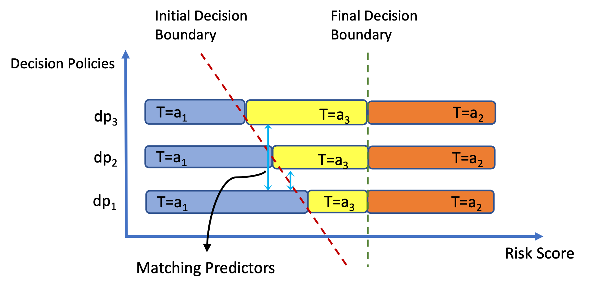
Figure 1: Decision policies across different locations

The proposed solution assumes there exist multiple locations with slightly different initial decision policies (dp) as shown in Figure 1. It represents a real-world scenario when some judges are strict and some are lenient [25]. The same is the case in child welfare, where some initial placement screenings are performed by police officers or by trained child welfare professionals [37] or state policies are different [28].

As mentioned earlier, the regressor $\tilde{\omega}_{a_{1}}(x)=\hat{\mathbb{E}}(Y|X,T=a_{1})$ will be erroneous due to confounding bias. However, in the case of randomized controlled trials (RCT), where $Y_{a_{1}}\perp T$, there will be no confounding bias for $\tilde{\omega}_{a_{1}}(x)$ even with hidden confounders [19]. Although observed samples from the whole population do not result from RCT, in data preprocessing, we only need to estimate $\hat{Y}_{a_{1}}$ for dual-treatment samples. By definition, dual-treatment samples are those for whom an erroneous decision was made initially and later reverted. In cases where we have varying decision boundaries between locations, the scope of samples with treatment $T=a_{1}$ from one location covers samples with treatment $T=a_{3}$ from another location, resembling an RCT between two treatments $a_{1}$ and $a_{3}$.

For instance, let’s consider there are three different decision policies (DPs) resulting in different decision boundaries for the initial decision as shown in Figure 1. It shows $dp_{1}$ is the lenient, and $dp_{3}$ is the strictest. Also, it is expected that the final decision boundary is uniform among locations since the review process is to ensure removing any biases in the judgment process. As a result, the scope of desired-treatment sample $T=a_{1}$ in $dp_{1}$ will cover the scope of dual-treatment samples $T=a_{3}$ in $dp_{2}$ and $dp_{3}$. Eventually when samples from all locations are considered as a whole, it will resemble a scenario of RCT between treatments $a_{1},a_{3}$ with $P(T=a_{1}|X,Z,T\neq a_{2})=P(T=a_{3}|X,Z,T\neq a_{2})\approx 0.5$.

The two subpopulations with treatments $a_{1}$ and $a_{3}$ satisfy $Y_{a_{1}}\perp T|T\neq a_{2}$. Thus, it is possible to correctly estimate potential outcome $\hat{Y}_{a_{1}}$ for dual-treatment samples from $\tilde{\omega}_{a_{1}}(x)$ . The detailed procedure is provided in Algorithm 1. First, it learns $\tilde{\omega}_{a_{1}}(x)=\hat{\mathbb{E}}(Y|T=a_{1},x)$, and then estimates potential outcome $\hat{Y}_{a_{1}}$ for dual-treatment samples. In Section 5.1, we have presented the effectiveness of this approach with varying CATE over synthetic data.

Algorithm 1 Label Estimation for dual-treatment samples

  Input: Data $D_{d\in\{dp_{1}...dp_{L}\}}=\{(X_{i},Z_{i},T_{i},Y_{i})\}_{i=1}^{n_{d}}$

  

  1. Train regressor $\tilde{\omega}_{a_{1}}(x)$ over $Y\sim X|T=a_{1}$

  2. Estimate $\hat{Y}_{a_{1}}$ from $\tilde{\omega}_{a_{1}}(x)$ for samples with $T=a_{3}$

  

  Return: Desired Labels $\hat{Y}_{a_{1}}$ for dual-treatment samples

4.2.2 Regression-Adjustment (RA) Predictor

In the Regression Adjustment (RA) method, target estimator $\hat{\nu}(x)$ is learned in two stages. The procedure is presented in Algorithm 2. First a nuisance estimator $\hat{\mu}_{a_{1}}(X,Z)=\hat{\mathbb{E}}(\hat{Y}_{a_{1}}|X,Z,T=a_{3})$ is learned with no confounding bias. Then similar to the semi-supervised learning approach the nuisance estimator will be used to provide a pseudo-outcome for the whole population. Then target model $\hat{\nu}(x)$ is estimated over the whole population using ground truth label for samples received treatment $T=a_{1}$ and pseudo outcome $\hat{\mu}_{a_{1}}(X,Z)$ for other samples with $T=\{a_{2},a_{3}\}$.

For theoretical error bounds, we have adopted a procedure similar to [21] which bounds the error for a two-stage regression on the full set of confounding variables.

Theorem 4.1.

Under sample-splitting to learn $\hat{\mu}_{a_{1}}(x,z)$, $\hat{\nu}(x)$, the RA method has pointwise regression error that is bounded by:

$$\mathbb{E}\Big{[}\big{(}\hat{\nu}(x)-\nu(x)\big{)}^{2}\Big{]}\lesssim\mathbb{E}\Big{[}\big{(}\tilde{\nu}(X)-\nu(X)\big{)}^{2}\Big{]}\\ +\mathbb{E}\Big{[}\big{(}\tilde{\mu}_{a_{1}}(x,Z)-\mu_{a_{1}}(x,Z)\big{)}^{2}|X=x\Big{]}\\ +\mathbb{E}\Big{[}\big{(}\Delta(x,Z)\big{)}^{2}|X=x\Big{]}$$

where $\hat{\nu}(x)$ is the final regressor. The right-hand side splits the error bounds according to the different stages of the algorithm, where $\tilde{\nu}(x)=\hat{\mathbb{E}}(\mathbb{I}_{a_{1}}Y+\mathbb{I}_{\neq a_{1}}\mu_{a_{1}}(X,Z)|X=x)$ denotes second-stage regression with oracle access to the first-stage output. $\tilde{\mu}_{a_{1}}(X,Z)=\hat{\mathbb{E}}(Y_{a_{1}}|X,Z)$ is the first stage regressor with oracle access to $Y_{a_{1}}$ and $\Delta(X,Z)=\mathbb{E}(\hat{Y}_{a_{1}}-Y_{a_{1}}|X,Z,T=a_{3})$ is the label estimation error for dual-treatment samples. Notably, the bound depend linearly on the Mean square error of $\tilde{\mu}_{a_{1}}(x,Z)$. The next approach provides a more robust mechanism by introducing another first-stage estimator.

Algorithm 2 Regression-Adjustment (RA) Algorithm

  Input: Data $D=\{(X_{i},Z_{i},T_{i},Y_{i})\}_{i=1}^{n}$

  

  Randomly divide $D$ into two partitions $W^{1},W^{2}$

  for (i,j) $\in$ {(1,2),(2,1)} do

     Stage 1: On $W^{i}$, learn regression function $\hat{\mu}_{a_{1}}(X,Z)$ over $\hat{Y}_{a_{1}}\sim X=x,Z=z|T=a_{3}$

     

     Stage 2: On $W^{j}$, learn regressor $\hat{\nu}^{j}(x)$ over $\mathbb{I}_{a_{1}}Y+\mathbb{I}_{\neq a_{1}}\hat{\mu}_{a_{1}}(X,Z)\sim X$

  end for

  

  Prediction: $\hat{\nu}(x)=\sum_{q=1}^{2}\hat{\nu}^{q}(x)$

4.2.3 Doubly-Robust (DR) Predictor

This method introduces two nuisance estimators, i.e. $\hat{\mu}_{a_{1}}(X,Z)$ and $\hat{\pi}_{a_{3}|\neq a_{1}}(X,Z)$. It guarantees robustness since it requires only one of the nuisance estimators to be closer to the true estimator. The DR method is presented in Algorithm 3. Again it’s a two-step procedure. At the first, it trains regressor $\hat{\mu}_{a_{1}}(X,Z)$ and conditional propensity score model $\hat{\pi}_{a_{3}|\neq a_{1}}(X,Z)$. The propensity score model allows us to estimate the likelihood of being a dual-treatment sample given it can not be a desired-treatment sample. Thus to train the propensity score model, no desired-treatment samples with $T=a_{1}$ are included. The second step of the DR algorithm involves training the target model $\hat{\nu}(x)$ over the whole population.

DR method provides better theoretical guarantees as compared to RA due to two nuisance estimators.

Theorem 4.2.

Under sample-splitting to learn $\hat{\mu}_{a_{1}}(x,z)$, $\hat{\nu}(x)$ and $\hat{\pi}_{a_{3}|\neq a_{1}}(x,z)$ the pointwise error bound for proposed DR method is given as:

$$\mathbb{E}\Big{[}\big{(}\hat{\nu}(x)-\nu(x)\big{)}^{2}\Big{]}\lesssim\mathbb{E}\Big{[}\big{(}\tilde{\nu}(x)-\nu(x)\big{)}^{2}\Big{]}\\ +\mathbb{E}\Big{[}\big{(}\tilde{\mu}_{a_{1}}(x,Z)-\mu_{a_{1}}(x,Z)\big{)}^{2}|X{=}x\Big{]}\\ \times\mathbb{E}\Big{[}\big{(}\hat{\pi}_{a_{3}|\neq a_{1}}(x,Z)-\pi_{a_{3}|\neq a_{1}}(x,Z)\big{)}^{2}|X{=}x\Big{]}\\ +\mathbb{E}\Big{[}\big{(}\Delta(x,Z)\big{)}^{2}|X{=}x\Big{]}$$

where $\hat{\nu}(x)$ is the final regressor and the error bound is split between different stages at the right-hand side. $\tilde{\nu}(x)$ denotes second-stage regressor with oracle access to true first-stage estimators ${\mu}_{a_{1}}(x,Z)$, ${\pi}_{a_{3}|\neq a_{1}}(x,Z)$. $\tilde{\mu}_{a_{1}}(x,Z)$ is the first stage regressor with oracle access to $Y_{a_{1}}$ and $\hat{\pi}_{a_{3}|\neq a_{1}}(x,Z)$ is the propensity score estimator. Finally, $\Delta(x,Z)=\mathbb{E}(\hat{Y}_{a_{1}}-Y_{a_{1}}|X,Z,T=a_{3})$ is the desired label estimation error for dual-treatment samples. Here, in the error bound there is a product between errors of nuisance estimators, which guarantees its robustness. The error bound still linearly depends on the label estimation error of dual-treatment samples. However, that estimation error over subpopulation is much simpler to handle as compared to the target problem of the whole population. Also, in some cases label estimation for dual-treatment samples might not be needed at all where $\text{CATE}(a_{1},a_{3})$ is negligible, as mentioned in Section 4.2.1.

Algorithm 3 Doubly-Robust (DR) Algorithm

  Input: $D=\{(X_{i},Z_{i},T_{i},Y_{i})\}_{i=1}^{n}$

  

  Randomly divide $D$ into three partitions $W^{1},W^{2},W^{3}$

  for (i,j,k) $\in$ {(1,2,3), (3,1,2), (2,3,1)}  do

     Stage 1: On $W^{i}$, train regression function $\hat{\mu}_{a_{1}}(X,Z)$ over $\hat{Y}_{a_{1}}\sim X=x,Z=z|T=a_{3}$

     

         On $W^{j}$, train conditional propensity estimator $\hat{\pi}_{a_{3}|\neq a_{1}}(X,Z)$ over $\mathbb{I}_{a_{3}}\sim X=x,Z=z|T\neq a_{1}$

     

     Stage 2: On $W^{k}$, train $\hat{\nu}^{k}(x)$ by regressing $\mathbb{I}_{a_{1}}Y+\mathbb{I}_{\neq a_{1}}\bigg{[}\frac{\mathbb{I}_{a_{3}}}{\hat{\pi}_{a_{3}|\neq a_{1}}(X,Z)}\big{(}\hat{Y}_{a_{1}}-\hat{\mu}_{a_{1}}(X,Z)\big{)}+\hat{\mu}_{a_{1}}(X,Z)\bigg{]}\sim X$

  end for

  

  Prediction: $\hat{\nu}(x)=\sum_{q=1}^{3}\hat{\nu}^{q}(x)$

5 Experiments

The evaluation of counterfactual prediction algorithms is challenging due to the absence of ground truth labels for subpopulations with different treatments. To overcome this challenge, counterfactual evaluation is typically performed using synthetic, semi-synthetic, or RCT data [45, 18]. In this study, we evaluated the proposed counterfactual prediction algorithms using both synthetic and real-world child placement data, and compared the results to the SP baseline approach. It is important to note that we are not aware of any other techniques that are both interpretable and able to predict under selective confounding, as discussed in Section 3.

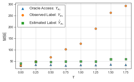
Figure 2: Performance under Varying Treatment Effects

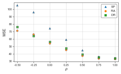
Figure 3: Performance Comparison over Confounders Correlation

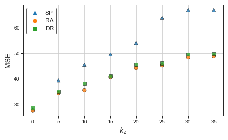
Figure 4: Performance comparison over Hidden-Confounders

5.1 Synthetic-Data Evaluation

Data: The synthetic data is generated for $L=20$ locations to simulate different decision policies. For each location, the acceptance rate between $ar=[0.3,0.5]$ is randomly picked which will determine how strict or lenient the initial decision policy is. Once determined, the acceptance rate will stay fixed for each location. There is $n=1000$ number of data points in each location.

The confounders $X,Z$ are sampled from Normal Distribution and the correlation among them is controlled using parameter $\rho$.

$$X_{i}\sim\mathbb{N}(0,1)\ \ ,\ Z_{i}\sim\mathbb{N}(\rho X_{i},1-\rho^{2})\ \ \ \ ;0\leq i\leq d$$

where $2*d$ is the total number of confounders present in a single sample. The potential outcome $\mu_{a_{1}},\mu_{a_{3}}$ under treatments $a_{1},a_{3}$ is determined by:

$$\mu_{a_{1}}(X,Z) =\frac{k_{x}}{k_{x}+\rho k_{z}}\left(\sum_{i=0}^{k_{x}}X_{i}+\sum_{i=0}^{k_{z}}Z_{i}\right)+\epsilon$$

$$\mu_{a_{3}}(X,Z) =\frac{k_{x}}{k_{x}+\rho k_{z}}\Big{[}\sum_{i=0}^{d}X_{i}+\sum_{i=0}^{d}Z_{i}$$

$$-\tau\big{(}\sum_{i=0}^{d}X_{i}+\sum_{i=0}^{d}Z_{i}^{2}\big{)}\Big{]}+\epsilon$$

with,

$$\epsilon\sim\mathbb{N}\big{(}0,\frac{1}{2n}\left\|\mu_{a_{1}}(X,Z)\right\|^{2}_{2})$$

and $k_{x},k_{z}$ determines the number of confounders impacting the outcome. CATE between two treatments $a_{1},a_{3}$ is controlled with parameter $\tau$. To compare learned estimator $\hat{\nu}(x)$, the ground truth outcome based on confounders $X$ is given as:

$$\nu(X)=\frac{k_{x}}{k_{x}+\rho k_{z}}\Big{[}\sum_{i=0}^{k_{x}}X_{i}+\rho\sum_{i=0}^{k_{z}}X_{i}\Big{]}$$

The propensity score, probability of treatment assignment, is given as $\pi(X,Z)$. To replicate real-world scenarios where decision reversal is possible through appeals and gives dual-treatment samples, we simulate two decision stages $d_{1},d_{2}$ corresponding to the initial and final decision.

$$\pi(X,Z)=\sigma\Big{(}\frac{1}{\sqrt{k_{x}+k_{z}}}\big{(}\sum_{i=0}^{k_{v}}X_{i}+\sum_{i=0}^{k_{z}}Z_{i}\big{)}\Big{)}$$

$$d_{1}=\text{Bernoulli}(min(\frac{\pi(X,Z)}{\text{ar}}*0.5,0.99))$$

$$d_{2}=\text{Bernoulli}(\pi(X,Z))$$

where $\sigma(x)=\frac{1}{1+e^{-x}}$ and $ar=[0.3,0.5]$ is the acceptance rate randomly picked for each location in the dataset. Lower $ar$ values mean a strict decision policy as it brings down the decision boundary from $0.5$. Based on $d_{1},d_{2}$, the assigned treatment is given as:

$$T=\left\{\begin{matrix}a_{1}&d_{1}=0\\ a_{2}&d_{1}=1\ \&\ d_{2}=1\\ \ a_{3}&d_{1}=1\ \&\ d_{2}=0\end{matrix}\right.$$

Metric: The dataset contain samples from all $L$ locations. For evaluation, the dataset is partitioned into train and test sets. The metric used to evaluate the performance of target estimator $\hat{\nu}(x)$ is Mean Square Error (MSE) given as:

$$\text{MSE}=\frac{1}{n}\sum_{i=1}^{n}\big{[}(\nu(x_{i})-\hat{\nu}(x_{i}))^{2}\big{]}$$ (1)

where $n$ is the total number points of points in the test set.

Results: Our solution comprises of two main components: 1) Estimation of potential outcome $\hat{Y}_{a_{1}}$ for dual-treatment samples using Algorithm 1 and 2) Training a counterfactual predictor model $\hat{\nu}(x)$ using RA (Algorithm 2) and DR (Algorithm 3) schemes.

Figure 4 demonstrates Algorithm 1’s effectiveness by comparing its performance over varying CATE($a_{1},a_{3}$) with three techniques for handling labels in dual-treatment samples. The estimator $\hat{\nu}(x)$ used only the DR scheme to ensure a fair comparison, and setting A in Table 1 was used for the experiment. The error lower bound is obtained with oracle access to potential outcome $Y_{a_{1}}$ for dual-treatment samples. Performance deteriorates with increasing $\tau$ when observed label $Y_{a_{3}}$ for dual-treatment samples is used without label estimation. However, when Algorithm 1 is used to estimate $\hat{Y}{a_{1}}$ for dual-treatment samples, performance does not degrade with $\tau$. Moreover, the proposed algorithm 1 performs similarly to using observed label $Y{a_{3}}$ as it is when the treatment effect is negligible (i.e., when $\tau\approx 0$). Thus, the proposed algorithm 1 can be used in any application with different values of $\tau$ without switching between label handling techniques.

Table 1: Experimental settings over synthetic-data

Setting	$d$	$k_{x}$	$k_{z}$	$\rho$	$\tau$
A	250	25	25	0.25	*
B	250	25	25	*	0.5
C	250	25	*	0.25	0.5

In Figure 4, we compare the final predictor approaches of AR and DR with the baseline SP, using Setting B given in Table 1. We plot their performances against the correlation $\rho$ between hidden and observed confounders. As $\rho$ increases, the observed features $X$ serve as proxies for $Z$. In such cases, SP performs comparably due to low confounding bias. However, when the correlation is low, there is a clear advantage of using counterfactual estimation approaches (AR, DR).

Figure 4 presents the impact of directly controlling confounding bias using $k_{z}$, with other parameter values set according to Setting C in Table 1. As expected, the performance of all algorithms decreases as the value of $k_{z}$ increases. However, the proposed counterfactual approaches, AR and DR, outperform the baseline SP, demonstrating their ability to effectively handle confounding bias during training.

It is important to note that in our experiments, there was no clear advantage of using the DR scheme over RA. While the DR scheme involves a more challenging training process for the conditional propensity score estimator ($\hat{\pi}_{{a_{3}}|\neq{a_{1}}}(x,z)$) compared to the outcome regressor $\hat{\mu}_{a_{1}}(x,z)$ used in RA, the DR scheme still provides robustness in case the outcome regressor fails to converge properly.

5.2 Real-World Data Evaluation

Data: The real-world data used in this study consists of placement decisions from eight states in the USA, with In-Home placement ($T=a_{1}$) as the desired treatment. While the eight locations cover a wide area with overlapping attributes, each state may handle cases differently. The observed features $X$ include demographics, case records, and complaints, while hidden features $Z$ include substantiated maltreatment, mental health, and disability type. The relevant outcome is whether or not further maltreatment occurred within six months of In-Home placement.

Figure 5 displays $N=5000$ samples randomly drawn from each location. As depicted in Figure 1, nearly similar proportions of Out-of-Home samples at each location led to a uniform final decision boundary. To compare the nature of sub-populations or the effectiveness of initial decision criteria among each state, two new metrics are introduced: Acceptance Rate (AR) and Failure Rate (FR), given as follows:

AR $$=\frac{\text{Number of In-Home samples}}{N}$$

FR $$=\frac{\text{Number of maltreated In-Home samples}}{N}$$

While a high AR usually results in a high FR and vice versa, not all states follow the same trend, as shown in Figure 5. This suggests that In-home sample distribution may vary among states, and certain states may have room for improvement in terms of FR.

Evaluation: To circumvent the issue of missing ground truth labels in evaluation, we have devised three new methods that are applicable in applications similar to child placement. The first method enables us to quantify the benefit of using a prediction model as compared to historical decision [25]. Meanwhile, the second and third methods allow us to compare different prediction models to select the best.

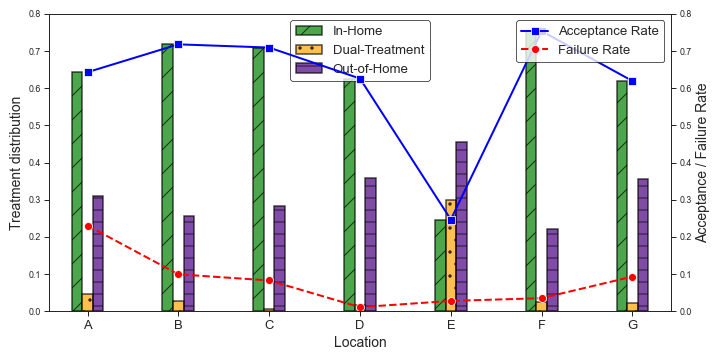
Figure 5: Real-World data Statistics

Method 1 - Comparison with Humans: In the child placement application, initial decisions may be wrong in two ways 1) higher FR among the In-home population, and 2) significant proportions of dual-treatment samples. For comparison, we see if the proposed prediction model (DR) can switch high-risk in-home samples with low-risk dual-treatment samples. The risk-score for dual-treatment samples can be estimated using Algorithm 1.

First using DR method, we estimate the risk score for the In-Home and dual-treatment samples. Then without modifying the AR of each location, assign In-Home treatment based on predicted risk scores of In-Home and dual-treatment samples. It can be seen in Figure 6, that prediction models bring down the FR for all locations. This improvement in FR is evident either for locations with a high proportion of dual-treatment samples like B,E,F, and G. Or, for a location where FR was already quite poor like A, B, C and G. After further analyses, we have discovered that the most common predictor responsible for short-stays is reported as child neglect [36], and our prediction algorithm rightfully assigns negative weightage to this predictor.

Method 2 - Evaluation over Outlier State: In Figure 5, AR and FR for different states are presented. Two locations, A and E, stand out with minimal difference between AR and FR. For evaluation purposes, location A is important due to its high FR. Its In-Home samples contain a significant number of high-risk samples that are usually Out-of-Home samples in other states. It allows us to train predictors over other locations B to F and evaluate them over In-Home samples of Location A. The results are reported in Table 2, and it can be seen that MSE is different between Standard Predictors (SP) and counterfactual predictors (RA, DR). First, it validates the evaluation method and also shows a gain in performance by circa 10% due to counterfactual predictors.

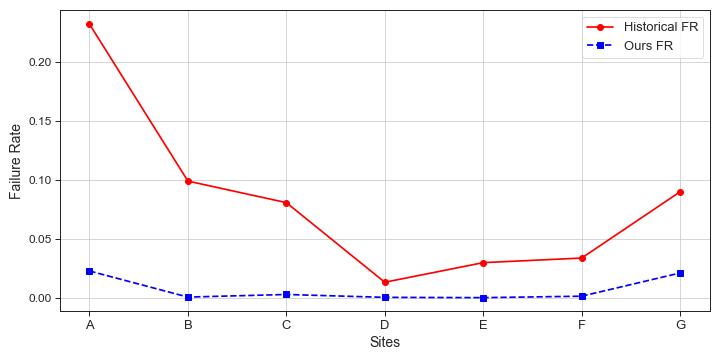
Figure 6: FR Comparison with Similar AR

Table 2: MSE Comparison from Proposed Evaluation Methods

Prediction Algorithm	Method 2	Method 3
Standard Predictor (SP)	0.8	0.83
Regression Adjustment (RA)	0.69	0.39
Doubly-Robust (DR)	0.68	0.26

Method 3 - Doubly-Robust Evaluation: The prediction error is identifiable when there are no hidden confounders under desired treatment as $\mathbb{E}((Y_{a_{1}}-\hat{\nu}(x))^{2}|X,Z)=\mathbb{E}((\hat{Y}_{a_{1}}-\hat{\nu}(x))^{2}|X,Z,T=a_{3})$. We propose the Doubly-Robust Evaluation approach similar to [10], with the difference that it can handle selective confounding. Our evaluation procedure identifies error term using dual-treatment samples. Defining identifiable error regressor as $\eta(X,Z):=\mathbb{E}((\hat{Y}_{a_{1}}-\hat{\nu}(x))^{2}|X,Z,T=a_{3})$, the doubly-robust estimate of MSE is given as:

$$\frac{1}{n}\sum_{i=1}^{n}\bigg{[}\mathbb{I}_{\neq a_{1}}^{i}\Big{[}\frac{\mathbb{I}_{a_{3}}^{i}}{\hat{\pi}_{a_{3}|\neq a_{1}}(X_{i},Z_{i})}\big{(}(\hat{Y}_{a_{1}}^{i}-\hat{\nu}(x_{i}))^{2}-\hat{\eta}(X_{i},Z_{i})\big{)}\\ +\hat{\eta}(X_{i},Z_{i})\Big{]}+\mathbb{I}_{a_{1}}^{i}(Y_{i}-\hat{\nu}(x_{i}))^{2}\bigg{]}$$

The results are reported in Table 2. It can be seen that there is a significant gain in using counterfactual predictors RA and DR as compared to SP. It is interesting to note that DR performs slightly better than RA which is highlighted by this method.

6 Summary

Counterfactual predictions for desired treatments play a crucial role in aiding decision-makers in real-world applications. However, assuming all confounders or their proxies are observable might not be realistic. In this work, we address this limitation by considering the scenario of selective confounding, where confounders can be hidden under a desired treatment. Despite this relaxation, our proposed method guarantees the identifiability of the target quantity and offers an interpretable target model, subject to two key assumptions: 1) The existence of different decision makers and 2) the possibility of appeal. To train the target model, we employ a two-stage counterfactual learning technique with no confounding bias. This allows us to use Linear Regression as the target model, making it inherently interpretable and suitable for societal applications. Our empirical results demonstrate that the proposed framework surpasses both human decision-makers and conventional statistical learning models in terms of performance. While we provide results for child-placement examples, the proposed method can be extended to other applications that satisfy the two conditions, such as ICU admission and police arrests.

Appendix A Appendix

A.1 Proof of Theorems

The theoretical results for our two-stage procedures relies on the theory for pseudo-outcome regression, which bounds the error for a two-stage regression on the full set of confounding variables during training [21, 10]. However, our setting is different due to confounded data in first stage. Let $D=(X,Z,T,Y)$ be the training data, split into two parts $D^{1}$ and $D^{2}$ to train first stage and second stage estimators respectively. Let $\hat{\mathbb{E}}_{n}(Y|X=x)$ be the estimator of regression function $\mathbb{E}_{n}(Y|X=x)$. The results assume the following two stability conditions on the second-stage regression estimators:

• Condition 1: $\hat{\mathbb{E}}_{n}(Y|X=x)+c\hat{\mathbb{E}}_{n}(Y+c|X=x)$ for any constant $c$.

• Condition 2: For any two random variables $R$ and $Q$ if $\mathbb{E}(R|X=x)=\mathbb{E}(Q|X=x)$, then

  $$\mathbb{E}\Big{[}\big{(}\hat{\mathbb{E}}_{n}(R|X=x)-{\mathbb{E}}(R|X=x)\big{)}^{2}\Big{]}\asymp\mathbb{E}\Big{[}\big{(}\hat{\mathbb{E}}_{n}(Q|X=x)-{\mathbb{E}}(Q|X=x)\big{)}^{2}\Big{]}$$

In our notations ${m}(x)=\mathbb{E}(f(Z)|X=x)$ represents the conditional expectation. $\tilde{m}(x)=\hat{\mathbb{E}}(f(Z)|X=x)$ represents oracle regression. $\hat{m}(x)=\hat{\mathbb{E}}(\hat{f}(Z)|X=x)$ represents regression over estimated $\hat{f}(Z)$.

Finally, the two-stage regressor error bound can be written as [21]:

$$\mathbb{E}\Big{[}\big{(}\hat{\nu}(x)-\nu(x)\big{)}^{2}\Big{]}\lesssim\mathbb{E}\Big{[}\big{(}\tilde{\nu}(X)-\nu(X)\big{)}^{2}\Big{]}\\ +\mathbb{E}\Big{[}\hat{r}(x)^{2}\Big{]}$$

Theorem 1:

$$\hat{r}(x) =\mathbb{E}_{D|X=x}\big{(}\mathbb{I}_{a_{1}}.Y+\mathbb{I}_{\neq a_{1}}.\hat{\mu}_{a_{1}}(x,Z)\big{)}-\mathbb{E}\big{(}\mu_{a_{1}}(x,Z)|X=x\big{)}$$

$$=\mathbb{E}_{Z,T|X=x}\Big{[}E_{Y|T=t,X=x,Z=z}\big{(}\mathbb{I}_{a_{1}}.Y+\mathbb{I}_{\neq a_{1}}.\hat{\mu}_{a_{1}}(x,Z)\big{)}\Big{]}-\mathbb{E}\big{(}\mu_{a_{1}}(x,Z)|X=x\big{)}$$

$$=\mathbb{E}_{Z,T|X=x}\Big{[}\big{(}\mathbb{I}_{a_{1}}.\mu_{a_{1}}(x,Z)+\mathbb{I}_{\neq a_{1}}.\hat{\mu}_{a_{1}}(x,Z)\big{)}\Big{]}-\mathbb{E}\big{(}\mu_{a_{1}}(x,Z)|X=x\big{)}$$

$$=\mathbb{E}_{Z,T|X=x}\Big{[}\big{(}\mathbb{I}_{a_{1}}.\mu_{a_{1}}(x,Z)+\mathbb{I}_{\neq a_{1}}.\hat{\mu}_{a_{1}}(x,Z)\big{)}\Big{]}-\mathbb{E}\big{(}\mathbb{I}_{a_{1}}\mu_{a_{1}}(x,Z)+\mathbb{I}_{\neq a_{1}}\mu_{a_{1}}(x,Z)|X=x\big{)}$$

$$=\mathbb{E}_{Z,T|X=x}\Big{[}\big{(}\mathbb{I}_{a_{1}}.\mu_{a_{1}}(x,Z)+\mathbb{I}_{\neq a_{1}}.\hat{\mu}_{a_{1}}(x,Z)-\mathbb{I}_{a_{1}}\mu_{a_{1}}(x,Z)-\mathbb{I}_{\neq a_{1}}\mu_{a_{1}}(x,Z)\big{)}\Big{]}$$

$$=\mathbb{E}_{Z,T|X=x}\Big{[}\big{(}\mathbb{I}_{\neq a_{1}}.\hat{\mu}_{a_{1}}(x,Z)-\mathbb{I}_{\neq a_{1}}\mu_{a_{1}}(x,Z)\big{)}\Big{]}$$

$$=\mathbb{E}_{Z,T|X=x}\Big{[}\big{(}\mathbb{I}_{\neq a_{1}}.\hat{\mathbb{E}}_{n}(\hat{Y}_{a_{1}}|X=x,Z=z)-\mathbb{I}_{\neq a_{1}}\mu_{a_{1}}(x,Z)\big{)}\Big{]}$$

$$=\mathbb{E}_{Z,T|X=x}\Big{[}\big{(}\mathbb{I}_{\neq a_{1}}.\hat{\mathbb{E}}_{n}(Y_{a_{1}}+\hat{Y}_{a_{1}}-Y_{a_{1}}|X=x,Z=z)-\mathbb{I}_{\neq a_{1}}\mu_{a_{1}}(x,Z)\big{)}\Big{]}$$

$$=\mathbb{E}_{Z,T|X=x}\Big{[}\mathbb{I}_{\neq a_{1}}\big{(}\tilde{\mu}_{a_{1}}(x,Z)+\Delta(x,Z)-\mu_{a_{1}}(x,Z)\big{)}\Big{]}$$

$$=\mathbb{E}_{Z|X=x}\Big{[}\pi_{\neq a_{1}}(x,Z)\big{(}\tilde{\mu}_{a_{1}}(x,Z)+\Delta(x,Z)-\mu_{a_{1}}(x,Z)\big{)}\Big{]}$$

$$\leq\mathbb{E}\Big{[}\big{(}\tilde{\mu}_{a_{1}}(x,Z)-\mu_{a_{1}}(x,Z)\big{)}|X=x\Big{]}+\mathbb{E}\Big{[}\Delta(x,Z)|X=x\Big{]}$$

The first line is the definition of error term $\hat{r}$ and the second line by iterated expectation. The third line uses the fact that only randomness inside is $Y$ and uses the definition of $\mu_{a_{1}}(x,Z)=\mathbb{E}(Y|X,Z,T=a_{1})$. The fourth line split second term among two populations. The fifth and sixth line rearranges terms and performs cancellation. The seventh line uses definition of $\hat{\mu}_{a_{1}}(x,z)$. Eighth line add and subtract $Y_{a}1$. The ninth line use definitions of $\tilde{\mu}_{a_{1}}(x,Z)$ and $\Delta(x,Z):=\hat{Y}_{a_{1}}-Y_{a_{1}}$. The tenth line performs iterated expectation $E_{T|X=x,Z=z}$ inside, where $T$ is the only random variable and applies definition of $\pi_{\neq a_{1}}(x,Z)=P(T\neq a_{1}|X,Z)$. The eleventh line ignores $\pi_{\neq a_{1}}(x,Z)$ to get the upper bound and rearranges the terms.

Taking square on both sides and using the fact $(a+b)^{2}\leq a^{2}+b^{2}$ gives:

$$\hat{r}(x)^{2}\leq\mathbb{E}\Big{[}\big{(}\tilde{\mu}_{a_{1}}(x,Z)-\mu_{a_{1}}(x,Z)\big{)}^{2}|X=x\Big{]}+\mathbb{E}\Big{[}\Delta(x,Z)^{2}|X=x\Big{]}$$

If $\hat{\mu}$ are estimated using separate training samples $D^{1}$, then taking the expectation over the first-stage training sample yields:

$$\mathbb{E}(\hat{r}(x)^{2})=\mathbb{E}\Big{[}\big{(}\tilde{\mu}_{a_{1}}(x,Z)-\mu_{a_{1}}(x,Z)\big{)}^{2}|X=x\Big{]}+\mathbb{E}\Big{[}\Delta(x,Z)^{2}|X=x\Big{]}$$

Theorem 2:

$$\hat{r}(x) =\mathbb{E}_{D|X=x}\Big{[}\mathbb{I}_{a_{1}}.Y+\mathbb{I}_{\neq a_{1}}.\big{\{}\frac{\mathbb{I}_{a_{3}}}{\hat{\pi}_{a_{3}|\neq a_{1}}(x,Z)}(\hat{Y}_{a_{1}}-\hat{\mu}_{a_{1}}(x,Z))+\hat{\mu}_{a_{1}}(x,Z)\big{\}}\Big{]}$$

$$\qquad\qquad\qquad\qquad\qquad\qquad\qquad\qquad\qquad\qquad\qquad\qquad-\mathbb{E}\big{(}\mathbb{I}_{a_{1}}\mu_{a_{1}}(x,Z)+\mathbb{I}_{\neq a_{1}}\mu_{a_{1}}(x,Z)|X=x\big{)}$$

$$=\mathbb{E}_{Z,T|X=x}\Big{[}E_{Y|T=t,X=x,Z=z}\ \ \mathbb{I}_{\neq a_{1}}.\big{\{}\frac{\mathbb{I}_{a_{3}}}{\hat{\pi}_{a_{3}|\neq a_{1}}(x,Z)}(Y_{a_{1}}+\Delta(x,Z)-\hat{\mu}_{a_{1}}(x,Z))+\hat{\mu}_{a_{1}}(x,Z)-\mu_{a_{1}}(x,Z)\big{\}}\Big{]}$$

$$=\mathbb{E}_{Z,T|X=x}\Big{[}\mathbb{I}_{\neq a_{1}}.\big{\{}\frac{\mathbb{I}_{a_{3}}}{\hat{\pi}_{a_{3}|\neq a_{1}}(x,Z)}(\mu_{a_{1}}(x,Z)-\hat{\mu}_{a_{1}}(x,Z)+\Delta(x,Z))+\hat{\mu}_{a_{1}}(x,Z)-\mu_{a_{1}}(x,Z)\big{\}}\Big{]}$$

$$=\mathbb{E}_{Z|X=x}\Big{[}\pi_{\neq a_{1}}(x,Z).\big{\{}\frac{\pi_{a_{3}|\neq a_{1}}(x,Z)}{\hat{\pi}_{a_{3}|\neq a_{1}}(x,Z)}(\mu_{a_{1}}(x,Z)-\hat{\mu}_{a_{1}}(x,Z)+\Delta(x,Z))+\hat{\mu}_{a_{1}}(x,Z)-\mu_{a_{1}}(x,Z)\big{\}}\Big{]}$$

$$=\mathbb{E}_{Z|X=x}\Big{[}\pi_{\neq a_{1}}(x,Z).\big{\{}\frac{1}{\hat{\pi}_{a_{3}|\neq a_{1}}(x,Z)}(\mu_{a_{1}}(x,Z)-\hat{\mu}_{a_{1}}(x,Z))(\pi_{a_{3}|\neq a_{1}}(x,Z)-\hat{\pi}_{a_{3}|\neq a_{1}}(x,Z))$$

$$\qquad+\frac{\pi_{a_{3}|\neq a_{1}}(x,Z)}{\hat{\pi}_{a_{3}|\neq a_{1}}(x,Z)}\Delta(x,Z)\big{\}}\Big{]}$$

$$\leq\mathbb{E}_{Z|X=x}\Big{[}\big{\{}\frac{1}{\hat{\pi}_{a_{3}|\neq a_{1}}(x,Z)}(\mu_{a_{1}}(x,Z)-\hat{\mu}_{a_{1}}(x,Z))(\pi_{a_{3}|\neq a_{1}}(x,Z)-\hat{\pi}_{a_{3}|\neq a_{1}}(x,Z))\big{\}}\Big{]}$$

$$\qquad\qquad\qquad\qquad\qquad\qquad\qquad\qquad\qquad\qquad\qquad\qquad+\mathbb{E}_{Z|X=x}\Big{[}\frac{\pi_{a_{3}|\neq a_{1}}(x,Z)}{\hat{\pi}_{a_{3}|\neq a_{1}}(x,Z)}\Delta(x,Z)\Big{]}$$

The first line uses the definition of $\hat{r}$. The second line rearrange terms, replace $\hat{Y}_{a_{1}}$ with $\hat{Y}_{a_{1}}+Y_{a_{1}}-Y_{a_{1}}$ and apply iterated expectation. In the third line only randomness inside is $Y$ and uses the definition of $\mu_{a_{1}}$. Fourth line uses iterated expecatation over $T$ and applies definition of $\pi_{t}$. The fifth and sixth lines simply rearrange terms.

By Cauchy-Schwarz Inequality and positivity assumption, we get:

$$\hat{r}(x)\leq C.\sqrt{\mathbb{E}[(\mu_{a_{1}}(x,Z)-\hat{\mu}_{a_{1}}(x,Z))^{2}|X=x]}\sqrt{\mathbb{E}[(\pi_{a_{3}|\neq a_{1}}(x,Z)-\hat{\pi}_{a_{3}|\neq a_{1}}(x,Z))^{2}|X=x]}+\mathbb{E}[\Delta(x,Z)|X=x]$$

where $C$ is constant. Then take square on both sides, and use the fact $(a+b)^{2}\leq a^{2}+b^{2}$ and apply Jensen’s Inequality on the second term.

$$\hat{r}(x)^{2}\leq{\mathbb{E}[(\mu_{a_{1}}(x,Z)-\hat{\mu}_{a_{1}}(x,Z))^{2}|X=x]}.{\mathbb{E}[(\pi_{a_{3}|\neq a_{1}}(x,Z)-\hat{\pi}_{a_{3}|\neq a_{1}}(x,Z))^{2}|X=x]}+\mathbb{E}[\Delta(x,Z)^{2}|X=x]\\$$

If nuisance estimator $\hat{\pi}$ and $\hat{\mu}$ are estimated using separate training samples, then taking the expectation over the first-stage training sample yields:

$$\mathbb{E}(\hat{r}(x)^{2})\leq{\mathbb{E}[(\mu_{a_{1}}(x,Z)-\hat{\mu}_{a_{1}}(x,Z))^{2}|X=x]}.{\mathbb{E}[(\pi_{a_{3}|\neq a_{1}}(x,Z)-\hat{\pi}_{a_{3}|\neq a_{1}}(x,Z))^{2}|X=x]}+\mathbb{E}[\Delta(x,Z)^{2}|X=x]\\$$

References

- [1] Alberto Abadie and Guido W Imbens, ‘Large sample properties of matching estimators for average treatment effects’, econometrica, (2006).
- [2] Charles Bhatti-Sinclair, Kish Sutcliffe, ‘Challenges in identifying factors which determine the placement of children in care? an international review’, Child and Adolescent Social Work Journal, (2013).
- [3] Ioana Bica, Ahmed M. Alaa, James Jordon, and Mihaela van der Schaar, ‘Estimating counterfactual treatment outcomes over time through adversarially balanced representations’, in 8th International Conference on Learning Representations ICLR, (2020).
- [4] Léon Bottou, Jonas Peters, Joaquin Quiñonero-Candela, Denis X. Charles, D. Max Chickering, Elon Portugaly, Dipankar Ray, Patrice Simard, and Ed Snelson, ‘Counterfactual reasoning and learning systems: The example of computational advertising’, Journal of Machine Learning Research (JMLR), (2013).
- [5] Tim Brennan, William Dieterich, and Beate Ehret, ‘Evaluating the predictive validity of the compas risk and needs assessment system’, Criminal Justice and Behavior, (2009).
- [6] Peter Bühlmann, Jonas Peters, and Jan Ernest, ‘Cam: Causal additive models, high-dimensional order search and penalized regression’, The Annals of Statistics, (2014).
- [7] Hugh A Chipman, Edward I George, and Robert E McCulloch, ‘Bart: Bayesian additive regression trees’, The Annals of Applied Statistics, (2010).
- [8] Ka Ho Brian Chor, Gary M. McClelland, Dana A. Weiner, Neil Jordan, and John S. Lyons, ‘Patterns of out-of-home placement decision-making in child welfare’, Child Abuse & Neglect, (2013).
- [9] Ka Ho Brian Chor, Gary M. McClelland, Dana A. Weiner, Neil Jordan, and John S. Lyons, ‘Out-of-home placement decision-making and outcomes in child welfare: A longitudinal study’, Administration and Policy in Mental Health and Mental Health Services Research, (2014).
- [10] Amanda Coston, Edward H. Kennedy, and Alexandra Chouldechova, ‘Counterfactual predictions under runtime confounding’, in 33: Annual Conference on Neural Information Processing Systems (NeurIPS), (2020).
- [11] Amanda Coston, Alan Mishler, Edward H. Kennedy, and Alexandra Chouldechova, ‘Counterfactual risk assessments, evaluation, and fairness’, in Proceedings of the Conference on Fairness, Accountability, and Transparency (FAT), (2020).
- [12] Michele Jonsson Funk, Daniel Westreich, Chris Wiesen, Til Stürmer, M. Alan Brookhart, and Marie Davidian, ‘Doubly robust estimation of causal effects’, American Journal of Epidemiology, (2011).
- [13] Zoe Getz, Cassandra Simmel, Liwei Zhang, and Brett Greenfield, ‘“short-stayers” in child welfare: Characteristics and system experiences’, Children and Youth Services Review, (2022).
- [14] Ruocheng Guo, Jundong Li, and Huan Liu, ‘Learning individual causal effects from networked observational data’, in Proceedings of the 13th International Conference on Web Search and Data Mining, WSDM ’20. Association for Computing Machinery, (2020).
- [15] Shonosuke Harada and Hisashi Kashima, ‘Infocevae: treatment effect estimation with hidden confounding variables matching’, Machine Learning, 1–19, (2022).
- [16] Jennifer L Hill, ‘Bayesian nonparametric modeling for causal inference’, Journal of Computational and Graphical Statistics, (2011).
- [17] Guido W. Imbens and Donald B. Rubin, Causal Inference for Statistics, Social, and Biomedical Sciences: An Introduction, Cambridge University Press, USA, 2015.
- [18] Fredrik D. Johansson, Uri Shalit, and David Sontag, ‘Learning representations for counterfactual inference’, in Proceedings of the 33rd International Conference on International Conference on Machine Learning (ICML), (2016).
- [19] Nathan Kallus, Aahlad Manas Puli, and Uri Shalit, ‘Removing hidden confounding by experimental grounding’, in Advances in Neural Information Processing Systems (NeurIPS), eds., S. Bengio, H. Wallach, H. Larochelle, K. Grauman, N. Cesa-Bianchi, and R. Garnett, (2018).
- [20] Nathan Kallus and Angela Zhou, ‘Confounding-robust policy improvement’, in Advances in Neural Information Processing Systems (NeurIPS), eds., S. Bengio, H. Wallach, H. Larochelle, K. Grauman, N. Cesa-Bianchi, and R. Garnett, (2018).
- [21] Edward H. Kennedy, ‘Optimal doubly robust estimation of heterogeneous causal effects’, arXiv: Statistics Theory, (2020).
- [22] Gary King and Richard Nielsen, ‘Why propensity scores should not be used for matching’, Political Analysis, 27(4), 435–454, (2019).
- [23] Toru Kitagawa and Aleksey Tetenov, ‘Who should be treated? empirical welfare maximization methods for treatment choice’, Econometrica, (2018).
- [24] Zhaobin Kuang, Frederic Sala, Nimit Sohoni, Sen Wu, Aldo Córdova-Palomera, Jared Dunnmon, James Priest, and Christopher Ré, ‘Ivy: Instrumental variable synthesis for causal inference’, in International Conference on Artificial Intelligence and Statistics. PMLR, (2020).
- [25] Himabindu Lakkaraju, Jon Kleinberg, Jure Leskovec, Jens Ludwig, and Sendhil Mullainathan, ‘The selective labels problem: Evaluating algorithmic predictions in the presence of unobservables’, in Conference on Knowledge Discovery and Data Mining (KDD), (2017).
- [26] Christos Louizos, Uri Shalit, Joris Mooij, David Sontag, Richard Zemel, and Max Welling, ‘Causal effect inference with deep latent-variable models’, in Proceedings of the 31st International Conference on Neural Information Processing Systems (NeurIPS), (2017).
- [27] David Madras, Elliot Creager, Toniann Pitassi, and Richard Zemel, ‘Fairness through causal awareness: Learning causal latent-variable models for biased data’, in Proceedings of the Conference on Fairness, Accountability, and Transparency (FAT), (2019).
- [28] Ferol E. Mennen, Matthew Brensilver, and Penelope K. Trickett, ‘Do maltreated children who remain at home function better than those who are placed?’, Children and youth services review, (2010).
- [29] Wang Miao, Zhi Geng, and Eric J Tchetgen Tchetgen, ‘Identifying causal effects with proxy variables of an unmeasured confounder’, Biometrika, (2018).
- [30] Judea Pearl, ‘Theoretical impediments to machine learning with seven sparks from the causal revolution’, Proceedings of the Eleventh ACM International Conference on Web Search and Data Mining, (2018).
- [31] James L. Peugh, ‘A practical guide to multilevel modeling’, Journal of School Psychology, (2010).
- [32] Yoshihiko Raita, Carlos Camargo, Liming Liang, and Kohei Hasegawa, ‘Big data, data science, and causal inference: A primer for clinicians’, Frontiers in Medicine, (2021).
- [33] James M. Robins, ‘Correcting for non-compliance in randomized trials using structural nested mean models’, Communications in Statistics - Theory and Methods, (1994).
- [34] Paul R. Rosenbaum and Donald B. Rubin, ‘The central role of the propensity score in observational studies for causal effects’, Biometrika, (1983).
- [35] Donald B Rubin, ‘Matching to remove bias in observational studies’, Biometrics, (1973).
- [36] Vivek S. Sankaran and Christopher E. Church, ‘Easy come, easy go: The plight of children who spend less than thirty days in foster care’, University of Pennsylvania Journal of Law and Social Change, (2016).
- [37] Vivek S. Sankaran, Christopher E. Church, and Monique T. Mitchell, ‘A cure worse than the disease? the impact of removal on children and their families’, Marquette Law Review, (2019).
- [38] Peter Schulam and Suchi Saria, ‘Reliable decision support using counterfactual models’, in Advances in Neural Information Processing Systems (NeurIPS), (2017).
- [39] Uri Shalit, ‘Can we learn individual-level treatment policies from clinical data?’, Biostatistics, (2019).
- [40] Rahul Singh, Maneesh Sahani, and Arthur Gretton, ‘Kernel instrumental variable regression’, Advances in Neural Information Processing Systems (NeurIPS), (2019).
- [41] Andrea C Skelly, Joseph R Dettori, and Erika D Brodt, ‘Assessing bias: the importance of considering confounding’, Evidence-based spine-care journal, (2012).
- [42] Peter Spirtes. A tutorial on causal inference, 2018.
- [43] Eric Tchetgen Tchetgen, ‘The control outcome calibration approach for causal inference with unobserved confounding’, American journal of epidemiology, (2014).
- [44] Stijn Vansteelandt and Marshall Joffe, ‘Structural Nested Models and G-estimation: The Partially Realized Promise’, Statistical Science, (2014).
- [45] Liuyi Yao, Zhixuan Chu, Sheng Li, Yaliang Li, Jing Gao, and Aidong Zhang, ‘A survey on causal inference’, Conference on Knowledge Discovery and Data Mining (KDD), (2021).
- [46] Weijia Zhang, Lin Liu, and Jiuyong Li, ‘Treatment effect estimation with disentangled latent factors’, Proceedings of the AAAI Conference on Artificial Intelligence, (2021).
- [47] Siyuan Zhao and Neil T. Heffernan, ‘Estimating individual treatment effect from educational studies with residual counterfactual networks’, in Educational Data Mining, (2017).
- [48] Min Zheng, Jessecae K. Marsh, Jeffrey V. Nickerson, and Samantha Kleinberg, ‘How causal information affects decisions’, Cognitive Research: Principles and Implications, (2020).