Caching Connections in Matchings

Abstract

Motivated by the desire to utilize a limited number of configurable optical switches by recent advances in Software Defined Networks (SDNs), we define an online problem which we call the Caching in Matchings problem. This problem has a natural combinatorial structure and therefore may find additional applications in theory and practice.

In the Caching in Matchings problem our cache consists of $k$ matchings of connections between servers that form a bipartite graph. To cache a connection we insert it into one of the $k$ matchings possibly evicting at most two other connections from this matching. This problem resembles the problem known as Connection Caching [20], where we also cache connections but our only restriction is that they form a graph with bounded degree $k$. Our results show a somewhat surprising qualitative separation between the problems: The competitive ratio of any online algorithm for caching in matchings must depend on the size of the graph.

Specifically, we give a deterministic $O(nk)$ competitive and randomized $O(n\log k)$ competitive algorithms for caching in matchings, where $n$ is the number of servers and $k$ is the number of matchings. We also show that the competitive ratio of any deterministic algorithm is $\Omega(\max(\frac{n}{k},k))$ and of any randomized algorithm is $\Omega(\log\frac{n}{k^{2}\log k}\cdot\log k)$. In particular, the lower bound for randomized algorithms is $\Omega(\log n)$ regardless of $k$, and can be as high as $\Omega(\log^{2}n)$ if $k=n^{1/3}$, for example. We also show that if we allow the algorithm to use at least $2k-1$ matchings compared to $k$ used by the optimum then we match the competitive ratios of connection catching which are independent of $n$. Interestingly, we also show that even a single extra matching for the algorithm allows to get substantially better bounds.

1 Introduction

We define the Caching in Matchings online problem, on a fixed set of $n$ nodes. Requests are edges between these node. The algorithm maintains a cache of $k$ matchings, i.e. a $k$-edge-colorable graph. To serve a request for an edge $(u,v)$ which is not in its cache (i.e. a miss), the algorithm has to insert it into one of its matchings. To do this it may need to evict the edges incident to $u$ and $v$ in this specific matching. Note that an evicted edge may later be re-inserted into a different matching. The algorithm has to choose which matching to use for each miss in order to minimize its total number of misses.

One can look at this problem as a new variation of the online Connection Caching problem. In Connection Caching [20] the setup is the same, but the cache maintained by the algorithm must be a graph in which each node is of degree at most $k$. In case of a miss on an edge $(u,v)$ we may choose any edge incident to $u$ and any edge incident to $v$ to evict. We do not have to maintain the edges partitioned into a particular set of $k$ matchings. Thus in Caching in Matchings we are less flexible in our eviction decisions. Once we color the new edge then the two edges we have to evict are determined.

At a first glance, the two caching problems seem similar. In fact, the only difference is the added restriction of the coloring (matchings) that affects how the cache is maintained. Interestingly, it turns out that this seemingly small difference makes Caching in Matchings a much harder online problem compared to Connection Caching.

A common measure to evaluate online algorithms is their competitive ratio. We say that an online algorithm is $c$-competitive if its cost (in our case, miss count) on every input sequence is at most $c$ times the minimal possible cost for serving this sequence. One would like to design algorithms with as small $c$ as possible. The problem of Connection Caching is known to be $\Theta(k)$ (deterministic) and $\Theta(\log k)$ (randomized) competitive, and in contrast we show that the dependence on $n$ (the number of nodes) in Caching in Matchings cannot be avoided.

The motivation to our Caching in Matchings problem comes from a data-center architecture described in [5]. In this setting we have $n$ servers connected via a communication network which is equipped with a set $O$ of $k$ optical switches. Each server is connected to all the $k$ optical switches and in each of them it is connected to both an input and an output port. Each switch is configured to implement a matching between the input and the output ports of the servers, see Figure 1. Since each server is connected to both input and output sides, the optical switches effectively induce a degree $k$ bipartite graph with $2n$ nodes (two nodes per server). Each optical switch corresponds to a matching in our cache. It is dynamic as we can insert and evict connections from the switch, but we try to minimize these reconfigurations since they are costly (involve shifting mirrors, and down-time).

At this point we clarify that there are two “kinds” of optical switching architectures. The one which we model, as explained, is based on off-the-shelf commodity switches and is sometimes referred to as Optical Circuit Switching (OCS). Each switch is a separate box, and each box, at any time, implements a matching between its ports. We use $k$ switches and connect every server to every switch, so this architecture induces $k$ matching at any time. To add a connection between two servers we have to choose through which box we want to do it (choose a matching to insert it to) and then reconfigure the matching implemented by this particular box to include this edge. The other kind of switching is known as Free Space Optics (FSO) where every transmitter can point towards any receiver. When each server is connected to $k$ transmitters and $k$ receivers we get the standard connection caching setting. This is not the architecture that we model here. See Table-1 of [26] for several references and their architecture types.

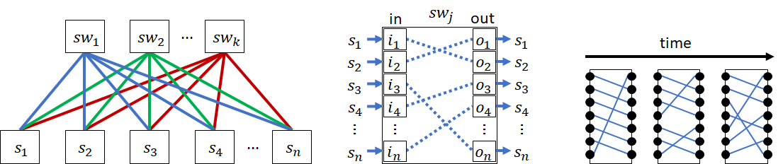
Figure 1: The physical topology that motivates our problem: $n$ servers $s_{1},\ldots,s_{n}$, each is connected to the in/out ports of $k$ optical switches ${sw}_{1}$ through ${sw}_{k}$. Each switch ${sw}_{j}$ uses mirrors to switch optical links, effectively inducing an in/out permutation, which may change over time at a reconfiguration cost of $1$ per each new pairing. Abstractly, we get a bipartite graph with $n$ nodes on each side (one per server), and each permutation is a matching that caches links.

Several cost models considering both communication and adjustment cost were suggested for this setting [5]. We choose to work with arguably the simplest model of paying $1$ for an insertion of a new edge (formally defined in Section 2). This simple model already captures the qualitative properties of the problem. We note that the competitive results shown here can be adapted (up to constant factors) to a more complicated cost model that has additional communication costs per request. We believe that our combinatorial abstraction of this setting is natural and will find additional applications.

Here is a detailed summary of our results.

Our contributions:

(1) We define a new caching problem, “Caching in Matchings” (Problem 1), on a bipartite graph with $n$ nodes on each side. In this problem, the cache is a union of $k$ matchings. When we insert an edge we pick the matching to insert it to and evict edges from this matching if necessary.

(2) We show that the competitive ratio of Caching in Matchings depends not only on the cache size $k$ as is common for caching problems, but also on the number of nodes in the network $n$. One might argue that since we define the cache to be $k$ matchings, its size is $\Theta(nk)$ rather than $k$, so the dependency on $n$ is not surprising. But such an argument also applies to Connection Caching [20] and in that problem the competitive ratio does not depend on $n$. In other words, Caching in Matchings is provably harder than Connection Caching. For the competitive ratios we prove an $\Omega(\max(\frac{n}{k},k))$ lower bound for deterministic algorithms and give a deterministic algorithm with $nk$ competitive ratio. This is tight for $k=O(1)$. In contrast, in the randomized case we have a larger gap. We describe an $O(n\log k)$ competitive algorithm and prove lower bounds of $\Omega(\log n)$ and $\Omega(\log\frac{n}{k^{2}\log k}\cdot\log k)$. The latter can get as worse as $\Omega(\log^{2}n)$ if $k=n^{1/3}$ (for example). This is in contrast to other caching problems whose randomized competitive ratio is a single logarithm (i.e., polylog of degree $1$).

(3) We show that resource augmentation of almost-twice as many matchings, specifically $2k-1$ for the algorithm versus $k$ for the optimum, allows to get rid of the dependence on $n$. Specifically, we show a deterministic $O(k)$ competitive algorithm and a randomized $O(\log k)$ competitive algorithm for this case. Furthermore, with $2(1+\alpha)k$ matchings we get a deterministic $O(1+\frac{1}{\alpha})$ competitive algorithm. We also show that a single extra matching already helps by allowing us to “trade” $\sqrt{n}$ for $\sqrt{k}$ in the competitive ratio. Concretely and more generally, with $h\geq 1$ extra matchings we get a deterministic $O(n^{1/2}(k/h)^{3/2})$ and a randomized $O(n^{1/2}(k/h)^{1/2}\log\frac{2k+h}{h})$ competitive algorithms.

Our problem is a special case of a more general problem of convex body chasing in $L_{1}$. Bhattacharya et al. [11] gave a general fractional algorithm for this body chasing problem with packing and covering constraints. Their fractional algorithm requires a slight resource augmentation. For a few special cases, they show how to round their fractional solution to an integral solution that does not use additional resources. Our problem is another interesting test-case of this general setting (see Appendix 6.3).

Our full list of results is summarized in Table 1. The rest of the paper is structured as follows. Section 2 formally defines the model, the notations that we use, and the caching problems. Section 3 studies in depth the Caching in Matchings problem (Problem 1). Section 4 surveys related work on caching and coloring problems, and in Section 5 we conclude and list a few open questions. Section 6 serves as an appendix that contains deferred proofs, and a few additional discussions.

2 Model and Definitions

In the following we formally define two caching problems of interest, the premise of each of them is a graph with a set $V$ of $n$ nodes. Every turn, a new edge is requested. If it is already cached, we have a “hit” and no cost is paid. Otherwise, we have a “miss”, and the edge must be brought into the cache at a cost of $1$, possibly at the expense of evicting other edges. In fact, the problem that arises from [5] consists of a bipartite graph in which each server $v$ is associated with two nodes $v^{in}\in V^{in}$ and $v^{out}\in V^{out}$, modeling its receiving and sending ports, respectively. Each among $v^{in}$ and $v^{out}$ can be incident to one edge in each matching. Formally the problem is as follows.

Problem 1 (Caching in Matchings).

Requests arrive for edges $(u,v)\in V^{in}\times V^{out}$. The cache $M$ is a union of $k$ matchings. When a requested edge is missing from all the matchings, an algorithm must fetch it into one of the matchings (possibly evicting other edges from this matching). In addition, the algorithm may choose to add any edge to the cache at any time (while maintaining the cache’s restrictions), the cost of adding an edge to the cache is $1$. It is not allowed to move an edge between matchings, but an edge may be evicted and immediately re-fetched into a new matching.

Remark 2.1.

There are other caching models in which reorganizing the cache is free, such as [17, 25]. In our model reorganizing the matchings incurs a cost. This is because we model a setting where changing the cache (physical links) is slow. In other cases accessing the slow memory is the costly operation.

We use the terminology of coloring edges when discussing Caching in Matchings (Problem 1). Recoloring an edge implies that we evict it, and then immediately fetch it back into a different matching according to the new color of the edge. Recoloring is not free, but has the same cost of standard fetching. This models, for example, the physical setting in which such a rearrangement requires reconfiguring the link in a different optical switch.

Problem 2 (Connection Caching [20]).

Requests arrive for edges $(u,v)\in V^{in}\times V^{out}$. The cache $M$ is a set of edges such that every node is of degree at most $k$ in the sub-graph induced by $M$. When a requested edge is missing from $M$, an algorithm must fetch it (possibly evicting other edges). In addition, the algorithm may choose to add any edge to the cache at any time (while maintaining the degrees at most $k$), the cost of adding an edge to the cache is $1$.

Remark 2.2.

Note that in both problems that we defined, an algorithm is allowed to add (fetch) and remove (evict) additional edges. Technically, it is not strictly necessary because a non-lazy algorithm can always be simulated by a lazy version that fetches an edge only when it is actually needed. This is also true for the offline optimum. That being said, we will describe non-lazy algorithms for Caching in Matchings, that recolor edges, to simplify the presentation.

To emphasize the difference between the problems see Figure 2, which shows the difference on bipartite graphs, as well as on general graphs (for the generalized problem).

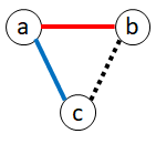
Figure 2: An example of the difference between connection caching versus caching in matchings. (left) With $k=2$ max degree and $n=3$ nodes, all the connections can be cached simultaneously, but not in $2$ matchings, red and blue. (right) Bipartite example: Caching the edge $(s^{i}_{1},s^{o}_{2})$ (i/o for in/out) is not possible without changing the matchings (red: $\{(s^{i}_{1},s^{o}_{3}),(s^{i}_{3},s^{o}_{1})\}$; blue: $\{(s^{i}_{3},s^{o}_{2}),(s^{i}_{2},s^{o}_{1})\}$), although both $s^{i}_{1}$ and $s^{o}_{2}$ only have a single connection.

The objective of an online algorithm is to minimize the number of fetched edges. The benchmark for evaluating the algorithms will be competitive-analysis.

Definition 2.3 (Cost, Competitive Ratio).

Consider a specific caching problem. Let $A$ be an online algorithm that serves requests, and let $\sigma$ be a sequence of requests. We denote by $A(\sigma)$ the execution of $A$ on $\sigma$, and $cost(A(\sigma))$ for the cost of $A$ when processing $\sigma$.

We denote by $OPT(\sigma)$ the optimum (offline) algorithm to serve the sequence, or simply $OPT$ when $\sigma$ is clear from the context. If there exist functions of the problem’s parameters (in our case: $k$ and $n$) $c=c(n,k)$ and $d=d(n,k)$ such that $\forall\sigma:cost(A(\sigma))\leq c\cdot cost(OPT(\sigma))+d$ then we say that $A$ is $c$-competitive. Note that $\sigma$ may be arbitrarily long, so the “asymptotic ratio” is indeed $c$.

Remark 2.4.

Denote the optima for Caching in Matchings and Connection Caching by $OPT_{m}$ and $OPT_{c}$, respectively. Since $OPT_{m}$ implicitly maintains connection caching (ignore the colors), then for any sequence of edge requests $\sigma$, $cost(OPT_{c}(\sigma))\leq cost(OPT_{m}(\sigma))$.

3 Caching in Matchings

In this section we study the problem of Caching in Matchings (Problem 1). We summarize the results of this section in Table 1. We start with upper bounds (Section 3.1), including those with resource augmentation, and then proceed to lower bounds (Section 3.2). Some additional discussion on randomization is deferred to the appendix (Section 6.3).

Result		Deterministic	Randomized	Notes
Cor. 3.4		$\leq nk$	$O(n\log k)$	The standard scenario
Cor. 3.4		$O(n^{1/2}(k/h)^{3/2})$	$O(n^{1/2}(k/h)^{1/2}\log\frac{2k+h}{h})$	RA: $k+h$ vs. $k$ for $h\geq 1$
Cor. 3.4	${*}$	$\leq k$	$O(\log k)$	RA: $2k-1$ vs. $k$
Thm. 3.4	${*}$	$O(1+\frac{1}{\alpha})$	.	RA: $(2+\alpha)k$ vs. $k$ for $\alpha>0$
Thm. 3.2	${*}$	.	$\Omega(\log\frac{n}{k^{2}\log k}\cdot\log k)$	.
Cor. 3.6	${*}$	$\Omega(max(\frac{n}{k},k))$	$\Omega(\log n)$	Due to Theorems 3.2+3.2
Cor. 3.6	${*}$	.	$\Omega(\epsilon\cdot\log n\cdot\log k)$	$k=O(n^{1/2-\epsilon})$; Due to Theorem 3.2

Table 1: Our bounds on the competitive ratio for Caching in Matchings (Problem 1), for $2\leq k<n$. If $k=1$ or $k\geq n$ optimality is trivial. Results marked with ${*}$ also apply to general graphs. RA is short for Resource-Augmentation, i.e., the algorithm has more matchings than the optimum.

3.1 Upper Bounds for Bipartite Graphs

In this section we prove upper bounds on the competitive ratio of algorithms for Caching in Matchings, focusing on the non-trivial case of $2\leq k\leq n-1$. Indeed, if $k=1$ there are no eviction-decisions to take so the only (lazy) algorithm is the optimal one. The other extreme case of $k\geq n$ in bipartite graphs is also easy since we can just cache the entire graph: Number the nodes $0$ to $n-1$ on each side, and use matching $i$ to store edges from node $j$ to $i+j$ modulo $n$.

Our general technique is to reduce the problem of Caching in Matchings to Connection Caching. Our algorithm, $A_{m}$, will run a Connection Caching algorithms $A_{c}$ with cache parameter $k$ to insert requested edges into the cache. Then, layered on top of $A_{c}$, we have the “coloring component” of $A_{m}$ that chooses the color of the new edge, and also recolors existing edges in order to produce a proper Caching in Matchings algorithm. The coloring component of $A_{m}$ uses a color-swap operation, of two (different) colors $c_{1}$ and $c_{2}$ with respect to a node $v$. The procedure looks at the bi-colored alternating path of edges of colors $c_{1}$ and $c_{2}$ that goes through a node $v$, and flips the color of every edge on this path. A color-swap maintains a proper edge coloring of the graph.

Observe that by the way $A_{m}$ is defined, it can be thought of as an edge coloring algorithm in the dynamic graph settings, and in this context $A_{c}$ is the adversary that tells $A_{m}$ which edges are inserted and which are removed (with a guarantee of bounded degree $k$). As a consequence we would like to use algorithms that are efficient in terms of recoloring, to achieve the best competitive results. Unfortunately, since edge coloring of graphs of bounded degree $k$ may require $k+1$ colors by Vizing’s theorem, the dynamic graph coloring literature studies this coloring problem while typically allowing more than $k$ colors. The number of extra colors ranges from $k+1$ colors [31], to $2k-1$ colors [10, 12], and sometimes even more [9, 32] (the last group of citations actually study vertex coloring). Extra colors correspond to resource augmentation, which we study too, in our simpler case of bipartite graphs.

Remark 3.1.

There are known algorithms that are $k$ competitive (deterministic) and $O(\log k)$ competitive (randomized) for Connection Caching, as studied in [20].

Due to Remark 2.4 and Remark 3.1, it suffices to analyze the cost ratio between $A_{m}$ and $A_{c}$. A ratio of $\rho$ implies a $\rho\cdot k$ deterministic and a $O(\rho\cdot\log k)$ randomized competitive algorithms for Caching in Matchings. We derive our competitive ratios from Theorem 3.1.

theoremtheoremUpperBoundReductionToCC Consider a bipartite graph with $n$ nodes on each side, and consider our algorithm $A_{m}$ that runs $A_{c}$, where the cache parameter of $A_{c}$ is $k$ and $A_{m}$ uses $x\geq k$ colors. Denote $\rho(x)\equiv\sup_{\sigma}{\frac{cost(A_{m}(\sigma))}{cost(A_{c}(\sigma))}}$ where $\sigma$ runs over all possible request sequences. Then: $\rho(k)\leq n$, $\rho(k+h)=O(\sqrt{nk/h})$ for $h\geq 1$, and $\rho(2k-1)=1$. ($\rho(2k-1)=1$ holds for general graphs.)

A proof sketch follows, the complete proof of Theorem 3.1 is deferred to Appendix 6.1.

Proof Sketch.

Whenever an edge $(u,v)$ is requested, $A_{m}$ has it cached if and only if $A_{c}$ has it cached. So for each $1$ paid by $A_{c}$, $A_{m}$ pays $1$ for coloring the new edge, plus the number of recolorings. Thus, to bound $\rho(x)$, it suffices to analyze the maximum such cost of $A_{m}$ per single missing edge of $A_{c}$. $u$ has some free color $c_{1}$ and $v$ has some free color $c_{2}$. There is only a problem if $c_{1}\neq c_{2}$. If $x=2k-1$ there is always a free common color for both $u$ and $v$ since each has (at least) $k$ different choices for the color of the new edge. If $x=k$ then we can apply a color-swap with respect to either $u$ or $v$ (the cheaper), of a path of length at most $n-1$. If $x=k+1$ we maintain a coloring such that no more than $O(\sqrt{nk})$ edges use the extra color. We use color-swaps in $u$, $v$, or both, to free this color if necessary. Once too many edges of this color exist, we fully recolor the graph. With $h\geq 1$ extra colors we generalize such that each extra color may have at most $O(\sqrt{nk/h})$ edges. When all fill up, we invoke a full recoloring. ∎

Next, we list three important facts about caching and connection caching algorithms, which we will use as $A_{c}$ to derive our matchings caching algorithm $A_{m}$, in a scenario of resource augmentation. Concretely, Lemma 3.2 details a concrete deterministic algorithm for Connection Caching, and Lemma 3.3 together with Theorem 3.3 yield a randomized algorithm for Connection Caching.

Lemma 3.2 (Corollary 8 of [20]).

There is a deterministic Connection Caching algorithm with cache of size $r$, that is $\frac{2r}{r-k+1}$-competitive against the optimum with cache of size $k\leq r$.

Lemma 3.3 (Section 2.2 of [34]).

Let $r$ be the cache size of the randomized caching algorithm MARK [24], and let $k$ be the cache size of the optimum. Then MARK is: $O(\log r)$-competitive if $r=k$; $O(\log\frac{r}{r-k})$-competitive if $\frac{e-1}{e}r<k<r$; and, $2$-competitive if $k\leq\frac{e-1}{e}r$.

[Theorem 7 of [20]]theoremtheoremDecouplingCCtoCaching Let $A$ be a $c(r,k)$-competitive caching algorithm, with additive term $\delta$, where $r$ and $k$ are the cache sizes of the algorithm and the optimum, respectively. Then there is a $2\cdot c(r,k)$-competitive algorithm for Connection Caching, with additive term $|V|\cdot\delta$ where $|V|$ is the number of nodes in the graph.

For completeness, we give the explicit reduction and proof of Theorem 3.3 in Appendix 6.4.

Corollary 3.4.

Consider the problem of Caching in Matchings:

1. There exist $nk$ deterministic and $O(n\log k)$ randomized competitive algorithms in bipartite graphs.

2. Resource augmentation of $h\geq 1$ extra matchings ($k+h$ versus $k$ for $OPT$) yields $O(n^{1/2}(k/h)^{3/2})$ deterministic and $O(n^{1/2}(k/h)^{1/2}\log\frac{2k+h}{h})$ randomized competitive algorithms in bipartite graphs.

3. Resource augmentation of extra $k-1$ matchings remove the dependence on $n$, yielding $k$ deterministic and $O(\log k)$ randomized competitive algorithms in general graphs.

We can improve the competitive ratio further with a larger resource augmentation.

theoremtheoremResourceAugmentationLargeDet Given $k+\Delta$ matchings to the algorithm compared to only $k$ matchings to the optimum, for $\Delta\geq k-1$, there is a deterministic algorithm that is $2(1+\frac{k-1}{\lfloor\frac{\Delta+3-k}{2}\rfloor})$-competitive for Caching in Matchings. In particular, with $\Delta=(1+\alpha)k$ extra matchings we get a competitive ratio of $O(1+\frac{1}{\alpha})$.

The proof is in Appendix 6.1. It follows from Theorem 3.1 (case $\rho(2k-1)$) and Lemma 3.2.

Corollary 3.5.

Consider the Caching in Matchings problem where the optimum is given $k$ matchings. There is a $6$-competitive algorithm that uses $3k-3$ matchings ($\Delta=2k-3$).

Note that all our algorithms for caching in matchings take $O(n)$ time per request: maintaining connection caching takes $O(k)$ time, and re-coloring a path of length $\rho$ takes $O(\rho)$ time, where $k\leq n$ by definition and $\rho\leq n$ by Theorem 3.1. We do not attempt to optimize further.

3.2 Lower Bounds

Caching in Matchings is a generalization of caching, if we restrict the requests to edges of a single fixed node. Observe, therefore, that any $c$-competitive online algorithm for Caching in Matchings with $2\leq k<n$ satisfies $c=\Omega(\log k)$. Moreover, if the algorithm is deterministic then $c\geq k$. The following lower bounds depend on $n$ as well as $k$. These bounds hold for the non-trivial case of $2\leq k<n$, in bipartite graphs, and therefore also hold for general graphs. Theorem 3.2 is proven later in this section, the proof of Theorem 3.2 is deferred to Appendix 6.2.

theoremtheoremLowerBoundDeterministic Any Deterministic Caching in Matchings algorithm is $\Omega(\frac{n}{k})$ competitive.

theoremtheoremLowerBoundRandLgNTimesLgK Any Caching in Matchings algorithm is $\Omega(\log\frac{n}{k^{2}\log k}\cdot\log k)$ competitive.

Corollary 3.6.

Any online algorithm for Caching in Matchings with $2\leq k<n$ is $\Omega(\log n)$ competitive. Moreover, if $k=O(n^{1/2-\epsilon})$ for some $\epsilon>0$, we get $\Omega(\epsilon\cdot\log n\cdot\log k)$ competitive. If the algorithm is deterministic then it is $\Omega(\max\{\frac{n}{k},k\})$ competitive.

Proof.

The deterministic claim follows from the initial observation and Theorem 3.2. In the general case (randomized), we get $\Omega(\log n)$ from the maximum between the observation (when $k\geq n^{1/3}$) and Theorem 3.2 (when $k<n^{1/3}$). The last part of the claim follows from Theorem 3.2: If $k\leq c\cdot n^{1/2-\epsilon}$ for some constant $c$ then $\log\frac{n}{k^{2}\log k}>\log\frac{n^{2\epsilon}}{c^{2}\log(cn)}=2\epsilon\log n-2\log c-\log\log(cn)=\Omega(\epsilon\cdot\log n)$. ∎

We prove the lower bounds in a setting that is closer to dynamic graph coloring. Specifically, we define Problem 3 below, where we control which edges must be cached both by the algorithm and the optimum. We prove (Lemma 3 below, proven in Appendix 6.2) that lower bounds for algorithms for Problem 3 imply lower bounds for Caching in Matchings, and then study lower bounds for Problem 3.

Problem 3.

Given a graph with $n$ vertices, we get a stream of actions that define a subset of edges at any time. Each action either adds a missing edge or deletes an existing edge.

We are guaranteed that at any point in time the graph induced by existing edges, denote it (or the set of edges) by $G$, has a proper $k$-edge-coloring. An algorithm, online or $OPT$, must maintain $k$ matchings, denote their union by $M$, such that $G$ is a subgraph of $M$. For every edge that is added to a matching, the algorithm pays $1$.

Note that Problem 3 is similar but not equivalent to dynamic edge coloring. On one hand a dynamic edge coloring algorithm that recolors $O(C)$ edges per update is not necessarily $O(C)$ competitive for Problem 3. The reason for this is that we allow $M$ to contain $G$. By maintaining an edge in $M$ we can avoid paying for it when it is inserted again. For example, in the proof of Theorem 3.2 the algorithm may do $O(1)$ worst-case recoloring per step, but the competitive ratio is $\Omega(\frac{n}{k})$ because $OPT$ stores in $M$ extra edges that the online algorithm keeps paying for. On the other hand, an algorithm that is $O(C)$ competitive for Problem 3 does not give a dynamic edge coloring algorithm that recolors $O(C)$ edges per update, even amortized, because it could be that both $OPT$ and the algorithm pay a lot per edge update on some sequence, and while the ratio is $O(C)$, the absolute cost is large.

lemmalemmaReductionToProblemStaticEdges A lower bound $C$ on the competitive ratio of an online algorithm for Problem 3 implies a lower bound $C$ on the competitive ratio of an online algorithm for Caching in Matchings.

We now focus on deriving lower bounds for Problem 3. We define a road gadget (Definition 3.8) which is a connected component with a large diameter, that is also very restricted in the way it can be colored. A road is constructed from brick sub-gadgets (Definition 3.7), each of size $\Theta(k)$ nodes and $\Theta(k^{2})$ edges. By connecting $r\geq 2$ roads together we get the $r$-road gadget, whose structure enforces those roads to be colored in a distinct and different way.

Definition 3.7 (Brick).

A colorless-brick is a union of $k$ perfect matchings on a bipartite graph with the following structure. Each side has $w$ nodes where $w$ is the unique power of $2$ that satisfies $\frac{w}{2}<k\leq w$. Number the nodes on each side $0,\ldots,w-1$, and number the colors $0,\ldots,k-1$. The matching of color $c$ matches node $i$ with node $i\oplus c$ where $\oplus$ is the bitwise exclusive-or. See Figure 3(a) for an example. Note that every color $c$ indeed defines a matching that is in fact a permutation of order $2$, and that $v\oplus c\neq v\oplus c^{\prime}$ for any two colors $c\neq c^{\prime}$ so the matchings are all disjoint.

When we remove an edge from a colorless-brick, we get a brick whose color is associated with the color of the non-perfect matching. The nodes of degree $k-1$ are the endpoints of the brick.

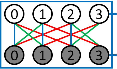
(a) Brick

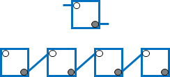
(b) Road

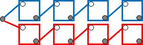
(c) $r$-Road for $r=2$

Figure 3: Visualization of a brick (Definitions 3.7), a road and an $r$-road (Definition 3.8). (a) A brick for $k=3$ ($w=4$). The number of each node is written, and the colors are as follows: blue (0), green (1), red (2). Thus, for example, $1\oplus red=3$. We removed a single edge, blue $(3,3)$, thus the brick is blue. (b) A schematic way to draw a brick (top) and a road of length $4$ (bottom) which is a chain of bricks connected to each other by their endpoints. The color of a road is well-defined by the color of its bricks. (c) An $r$-road for $r=2$, of length $4$. The node that connects to both roads is the hub of this $2$-road. Nodes are colored by gray and white according to their side in the bipartite graph.

Definition 3.8 (Road, $r$-road).

A road of length $d\geq 1$ is an edge colored graph obtained by connecting a sequence of $d$ bricks. Each brick is connected by an edge to the next brick in the sequence. The edge connecting two consecutive bricks is adjacent to an endpoint of each brick. Note that the color of two connected bricks must be the same since they must agree on their free color which is the color of the edge which connects them. Therefore, we define the color of a road to be the color of its bricks. A road has two ends, which are the endpoints of its first and last bricks. We also refer to $r$ ($2\leq r\leq k$) roads of the same length $d$ that are all connected to a single shared node as an $r$-road of length $d$. The shared node is its hub. The edges of the hub all have different colors, therefore all the roads of an $r$-road have different colors. See Figure 3 for examples.

In the remainder of this section we prove the deterministic lower bound. The randomized lower bound, proven in Appendix 6.2, uses the same gadgets but with a somewhat different approach.

Lemma 3.9.

Given a brick $B$ of color $c_{1}$, and a new color $c_{2}\neq c_{1}$, it is always possible to recolor $3$ edges to change the color of $B$ to $c_{2}$.

Note that when we recolor $B$, it no longer satisfies the $\oplus$-property of Definition 3.7, but for convenience we still consider it as a brick. This would not affect our arguments below (by more than a constant factor) since we will make sure to always return to the original coloring (undo) before recoloring again.

Proof.

Denote by $u$ one endpoint of the brick. By definition of the matching scheme, the other endpoint is $u\oplus c_{1}$, and when we restrict the graph to only edges of colors $c_{1}$ and $c_{2}$, we find that the path between $u$ and $u\oplus c_{1}$ is of length $3$: $u\oplus c_{1}\to u\oplus c_{1}\oplus c_{2}\to u\oplus c_{2}\to u$. Therefore, it suffices to flip the color of these three edges from $c_{2}$ to $c_{1}$ and vice versa. ∎

Proof of Theorem 3.2.

We prove the lower bound for Problem 3. Then the theorem follows by Lemma 3. We present an adversarial construction against a given algorithm $ALG$.

We begin by setting aside one special node $u$ to serve as a $2$-road hub, and divide the rest of the vertices into bricks. We construct from these bricks the longest possible road, of length $N=\Theta(\frac{n}{k})$. We number the bricks in order, from $1$ to $N$, and denote the edge between bricks $i$ and $i+1$ by $(i,i+1)$. Let $L=\lfloor\frac{N}{3}\rfloor$. Initially we insert all the edges of all the bricks, without the edges connecting the bricks. These edges are never deleted. Our sequence has as many steps as we like as follows, based on the state of $ALG$, see also Figure 4:

1. Simple step: If there exist consecutive bricks $i$ and $i+1$ of different colors, we insert the edge $(i,i+1)$. This forces $ALG$ to recolor at least one of the bricks and pay $\Omega(1)$ (it could pay more if it recolors more bricks or does other actions). We then delete $(i,i+1)$.

2. Split step: Otherwise, all the bricks of $ALG$ have the same color. We insert all the edges between bricks $1$ through to $L$, and between $N+1-L$ through to $N$. We also insert edges from $u$ to bricks $1$ and $N+1-L$. These insertions construct a $2$-road with $u$ as its hub, that guarantees different colors for bricks $1$ to $L$ compared to bricks $N+1-L$ to $N$. $ALG$ must recolor at least $L=\Omega(N)$ bricks. We then delete the edges that we inserted.

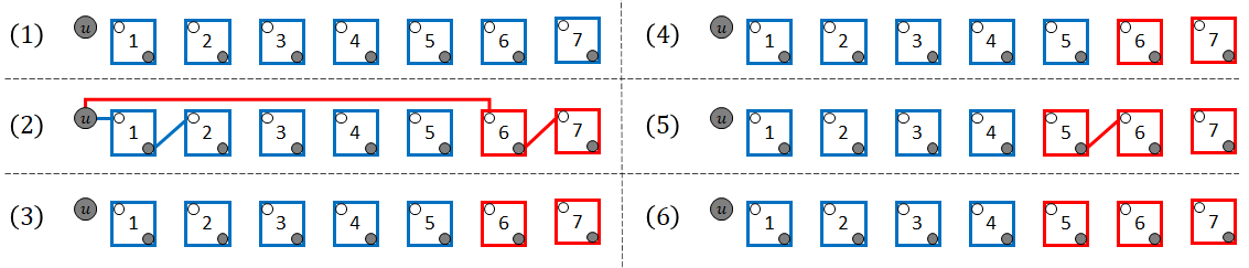
Figure 4: Visualization for the proof of Theorem 3.2, for $N=7$, $L=\lfloor\frac{N}{3}\rfloor=2$. (1)-(3) A split step temporarily creates a $2$-road of length $L$ out of the first and last bricks, with $u$ as the hub, to guarantee consecutive bricks with different colors. (4)-(6) A simple step finds two consecutive bricks with different color (here: $5$ and $6$), and inserts temporarily the edge between them to enforce recoloring of one of them.

In simple terms, we maintain a hole in the road which is where the color of the bricks changes (there could be multiple holes). In every step we request this hole, and once the hole disappears, the split action re-introduces a hole back near the middle of the road.

Now let us analyze the costs. If the sequence contains $m$ simple steps and $s$ split steps, then $cost(ALG)=\Omega(m+s\cdot N)$. For $OPT$, we define a family of strategies $B_{i}$ for $L<i<N+1-L$, to bound its cost. We define $B_{i}$ to store all the edges of all the bricks, all the edges connecting them, and the edge that connects $u$ to the first brick, except for the edges that connect brick $i$ to its neighbours, paying an initial $O(N\cdot k^{2})$ cost. $B_{i}$ colors all the bricks from $1$ to $i$ in one color, and all the bricks from $i+1$ to $N$ in another color. Whenever a simple step happens in $(i-1,i)$ or in $(i,i+1)$, $B_{i}$ simply recolors brick $i$ to have the same color of the neighbour it connects to, and also inserts the connecting edge. Simple steps at other locations do not affect $B_{i}$. When a split step happens, $B_{i}$ pays exactly $2$: It inserts the edge that connects $u$ to brick $N+1-L$ instead of the edge $(N-L,N+1-L)$. When the split step ends, it undoes the change, re-inserting $(N-L,N+1-L)$ instead of the edge of $u$. Since $L<i<N+1-L$, $B_{i}$ does not have to recolor any other edge.

Thus, if we denote by $m_{i}$ the number of simple steps that insert the edge $(i,i+1)$, then $cost(OPT)\leq cost(B_{i})=O(m_{i}+m_{i-1}+s+N\cdot k^{2})$. Now: $\frac{N}{3}\cdot cost(OPT)\leq(N-2L)\cdot cost(OPT)\leq\sum_{i=L+1}^{N-L}{cost(B_{i})}=O(m+N\cdot s+N^{2}k^{2})$. Note that $N^{2}k^{2}=O(n^{2})$. Thus by extending the sequence such that $m+s=\Omega(n^{2})$, we get: $\frac{N}{3}\cdot cost(OPT)=O(m+N\cdot s)=O(cost(ALG))$. Therefore, $\frac{cost(ALG)}{cost(OPT)}=\Omega(N)$. Recall that $N=\Theta(\frac{n}{k})$, and the claim follows. ∎

4 Related Work

Caching Problems: Caching problems have been studied in many variants and cost models. Connection caching is the caching variant closest to our problem. We presented it in a centralized setting, Cohen et al. [20] introduced it in a distributed setting. Albers [4] studies generalized connection caching. Bienkowski et al. [14] study connection caching in a cost model that is similar to that of caching with rejections [23]. Another related variant is restricted caching [17, 25] where not every page can be put into every cache slot. Buchbinder et al. [17] study the case where each page $p$ has a subset of cache slots in which it can be cached. In our problem we also have a restriction of similar flavour, implied by the separation into matchings. We note that the cost model in [17, 25] only counts cache-misses, while we also pay for rearranging the cache.

Linear Programming and Convex Body Chasing in $L_{1}$: The aforementioned caching problems, like many other combinatorial problems, can be formulated as a linear program [18]. This line of research led to the development of competitive algorithms for weighted and generalized caching [1, 2, 7, 8]. A recent result of Bhattacharya et al. [11] uses linear programming with packing and covering constraints to formulate and frame the problem as convex body-chasing in $L_{1}$. They give a fractional algorithm that requires a slight resource augmentation, along with some rounding schemes to get randomized algorithms for specific problems. Our problem can be thought of as another special case of the problem considered by [11], see Appendix 6.3 for this formulation and further details.

Coloring Problems: As mentioned in Section 3.1, efficient dynamic edge coloring that uses a small number of colors can be useful for competitive analysis. Unfortunately, graph coloring is usually studied in a more general context that typically allows $k+1$ or more colors [10, 12, 31] where $k$ in this context is the maximum degree in the graph. Vertex coloring results [9, 13, 27, 28, 30, 32] can technically be applied to obtain edge coloring by coloring the line-graph, but they too require extra colors. A deeper issue with this reduction to coloring the line-graph is that while it is $k$ colorable, its maximum degree is $2k-2$, and a generic vertex coloring algorithm will assume at least $2k-1$ colors at its disposal. The work [27] vertex-colors graphs based on their arboricity instead of the maximum degree. However, they require a number of colors that is a large multiple of the arboricity, $O(\log n)$ (where $n$ is the number of nodes), therefore we cannot use this coloring for our problem. Indeed, the arboricity of our line-graph can get as high as $k$ (see Appendix 6.4, Lemma 6.8). There are also works on maintaining dynamically an implicit coloring of the graph, by providing an efficient (and consistent) color-query function instead of storing the explicit coloring [19, 27]. This model cannot apply to our case because the matchings form an explicit coloring.

The area of dynamic coloring usually studies the tradeoffs between the number of colors being used, the amount of recoloring per graph update, and the update’s running time. El-Hayek et al. [22] study $b$-matchings and fully dynamic $k$-edge-coloring, with the objective to maximize, online, the number of colored edges at any given time. The work of Azar et al. [6] study dynamic vertex coloring in the context of competitive analysis where the objective is to minimize the total cost of recoloring.

5 Conclusions and Future Work

In this paper we studied the online Caching in Matchings problem, in which we receive requests for edges in a graph and need to maintain a cache of the edges which is a union of $k$ matchings. The problem abstracts some hardware architecture in which a datacenter is enhanced with reconfigurable optical links. Interestingly, we proved that the Caching in Matchings problem is inherently harder than the similar-looking Connection Caching problem and other caching problems. Specifically, its competitive ratio depends not only on the number of matchings $k$ (“cache size”) but also on the number of nodes in the graph. Our randomized lower bound rules out an $O(\log n)$ competitive algorithm, and the best competitive ratio we can hope for is $O(poly(\log n))$. Our lower bound for deterministic algorithms is linear in $n$.

We derived our algorithms by running a coloring algorithm that maintains a coloring of the cache of a connection caching algorithm. This approach is simple to describe and analyze, but inherently multiplies the competitive ratios of the two algorithms. It is natural to ask whether a “direct” algorithm for Caching in Matchings exists, and if so does it improve the competitive ratio?

Regarding resource augmentation, the bound of $O(\sqrt{nk/h})$ of Theorem 3.1 on the recoloring of an algorithm that has $k+h$ matchings depends on $n$ for $h=k-1$ if $k=o(n)$. However, the same theorem shows that for $h=k-1$ we get a simple algorithm without recolorings, whose competitive ratio is independent of $n$ and even equal to the bound of regular connection caching. This suggests that either there is an inherent discontinuity between $h=k-2$ and $h=k-1$, or that our bounds are not tight. This begs the question: Is there an algorithm with a better competitive ratio for $1\leq h<k-1$? Is there an $1\leq h<k-1$ and an algorithm that uses $h$ extra matchings with a competitive ratio of $O(poly(\log n))$?

A natural generalization would be to study upper bounds of Caching in Matchings in general graphs. When $k=1$ optimality is still trivial, and when $k=n$, by Vizing’s theorem, we are also optimal since we can edge-color the full $n$-clique with $n$ colors. In fact, for $n\geq 2$, $k=n-1$ colors are sufficient if and only if $n$ is even. In the non-trivial regime $2\leq k<n$, there exists a naive deterministic $O(n^{2}k^{2})$ competitive algorithm (Lemma 6.9 in Appendix 6.4). Resource augmentation of an extra matching ($k+1$ colors) dramatically reduces the competitive ratio to $O(nk)$ (deterministic) and $O(n\log k)$ (randomized) by allowing us to update the coloring of the graph when a new edge is inserted according to a single step of the Misra-Gries algorithm [31]. It is an interesting question whether the problem is indeed that much harder in general graphs. General graphs also provide additional difficulties, such as the fact that finding minimal edge coloring for $k\geq 3$ is generally NP-complete [29].

6 Appendix: Deferred Proofs and Discussions

6.1 Caching in Matchings Upper Bounds (Proofs)

In this section we restate and prove the claims from Section 3.1 that we did not prove there.

*

Proof.

Whenever an edge $(u,v)$ is requested, $A_{m}$ has it cached if and only if $A_{c}$ has it cached. Therefore when $A_{m}$ has a miss, so does $A_{c}$. To accommodate for the edge, $A_{c}$ ensures that $u$ and $v$ are both of degree $k-1$ before $(u,v)$ is inserted. Now we consider how much recoloring of edges may be required to ensure that $A_{m}$ can legally insert and color the edge.

If $A_{m}$ has $2k-1$ colors, then each of $u$ and $v$ has at least $k$ free colors. But there are $2k-1$ colors in total, so their free colors must overlap by at least one color, which means that $A_{m}$ does not need to recolor any edge if it simply inserts the new edge with the common free color. Therefore, $\rho(2k-1)=1$. Note that this part of the claim holds for general graphs.

If $A_{m}$ has $k$ colors, then both $u$ and $v$ each has at least one free color, since their degree is at most $k-1$. If both have some free color $c$, we are done. Otherwise, $u$ has $c_{1}$ free and $v$ has $c_{2}\neq c_{1}$ free. We apply a color-swap of $c_{1}$ and $c_{2}$, with respect to either $v$ or $u$ depending which is cheaper. Since $G$ is bipartite we can then safely insert $(u,v)$. Indeed, $(u,v)$ cannot close an (even) cycle with the path of the color-swap since this contradicts the fact that $c_{1}\neq c_{2}$. Since $(u,v)$ connects two paths into a longer path whose length is at most $2n-1$ edges (at most $n$ edges of each color, and not a cycle), the shorter path plus $(u,v)$ are at most $n$ edges in total, and we get that $\rho(k)\leq n$.

For the claim of $k+h$ colors, first consider $h=1$. If $A_{m}$ has $k+1$ colors we use the extra color, referred to as yellow, to ensure short swaps. We allow at most $y$ yellow edges in the graph, and if we need more, we recolor the whole graph from scratch without using yellow. Such a recoloring is possible because the graph is bipartite and every node is of degree at most $k$. When coloring a newly inserted edge $(u,v)$ we have three cases:

1. If $u$ and $v$ share a free color, including yellow: Then use this color.

2. If $u$ does not have a yellow edge and $v$ does (the other case is symmetric): Let $c$ be a free color of $v$, and apply a color-swap of $c$ and yellow with respect to $v$. This makes yellow a free color of $v$. Note that $u$ is unaffected by the color-swap, because the graph is bipartite (affecting $u$ implies that the path of the swap closes an odd cycle with the edge $(u,v)$). Now color $(u,v)$ in yellow.

3. If both $u$ and $v$ have a yellow edge: Let $c$ be a free color of $u$. Apply a color-swap of $c$ and yellow with respect to $u$. This makes yellow a free color of $u$. Now apply the previous case ($v$ will still have a yellow edge at this point, even if it is on the path affected by $u$).

We apply up to two color-swaps. Each of these swaps is of length $O(y)$ because there are at most $y$ yellow edges in the whole graph. So, $A_{m}$ pays $O(y)$ more than $A_{c}$ in “local” actions. Recall that we might have a global recoloring once we reach $y$ yellow edges. We charge these recolorings to the yellow edges. Formally, we define a potential for the cache which equals $\frac{nk}{y}\cdot i$ when there are $i$ yellow edges. Thus when we accumulate $y$ yellow edges, the potential can pay for the global recoloring. Each request causes $O(y)$ work and increases the potential by at most $\frac{nk}{y}$, due to possibly inserting a yellow edge (our color-swaps never increase the number of yellow edges). We conclude that the amortized cost of $A_{m}$ is $O(y+\frac{nk}{y})$ per miss of $A_{c}$. Balancing with $y=\sqrt{nk}$, we get $\rho(k+1)=O(\sqrt{nk})$.

We can generalize the previous logic for $h\geq 1$. We allow each extra color to have at most $y$ edges, and when it fills up we proceed to use the next extra color. Only when all $h$ colors have $y$ edges we invoke a full recoloring. The potential in this case is $\frac{nk}{hy}$ per edge, and the amortized cost per miss of $A_{c}$ is therefore $O(y+\frac{nk}{hy})$. Balancing with $y=\sqrt{nk/h}$, we get $\rho(k+h)=O(\sqrt{nk/h})$. ∎

*

Proof.

Let $\sigma$ be a sequence of requests. Denote an algorithm $A$ with cache parameter $x$ as $A^{x}$, and use subscripts $m$ for Caching in Matchings and $c$ for Connection Caching. By Theorem 3.1, $cost(A_{m}^{2r-1}(\sigma))=cost(A_{c}^{r}(\sigma))$ for any integer $r\geq 1$. Since this reduction halves the cache parameter, and our algorithm initially has cache of size $k+\Delta$, we use $r=\lfloor\frac{k+\Delta+1}{2}\rfloor$. If $k+\Delta=2r$, we do not use one of the colors, on purpose, to ensure using exactly $2r-1$ colors. Taking $A_{c}$ to be the algorithm that satisfies Lemma 3.2, $cost(A^{r}_{c}(\sigma))\leq\frac{2r}{r-k+1}\cdot cost(OPT^{k}_{c}(\sigma))+d$ for some fixed term $d$. By Remark 2.4, $cost(OPT^{k}_{c}(\sigma))\leq cost(OPT^{k}_{m}(\sigma))$. Plugging everything together we get that $cost(A^{2r-1}_{m}(\sigma))\leq\frac{2r}{r-k+1}\cdot cost(OPT^{k}_{m}(\sigma))+d$, hence $A^{2r-1}_{m}$ is $\frac{2r}{r-k+1}=2(1+\frac{k-1}{r-k+1})=2(1+\frac{k-1}{\lfloor\frac{\Delta+3-k}{2}\rfloor})$ competitive for Caching in Matchings. ∎

6.2 Caching in Matchings Lower Bounds (Proofs)

In this section we restate and prove the claims from Section 3.2 that we did not prove there.

*

Proof.

Let $A_{1}$ be a $c$-competitive algorithm for Caching in Matchings (Problem 1), with some additive term $d$. We show how to derive from it an algorithm $A_{3}$ that is $c$-competitive for Problem 3, which proves the claim. We will also use corresponding subscripts $OPT_{1}$ and $OPT_{3}$ for the optimum of each problem (with respect to a given sequence).

Given a sequence $\tau$, Algorithm $A_{3}$ takes its decisions while processing $\tau$ by simulating $A_{1}$ on a sequence $\sigma$ which is constructed as follows. We traverse $\tau$ in order, and whenever an edge is inserted, we add to $\sigma$ a batch of requests which is a concatenation of $r=nk$ identical subsequences, each subsequence contains all the edges currently in $G$ (in some arbitrary order). When an edge is deleted, we do nothing.

We now specify $A_{3}$ such that $cost(A_{3}(\tau)))\leq cost(A_{1}(\sigma))$ by having $A_{3}$ maintain its state such that it “jumps” between “check-points” in the state of $A_{1}$.

$A_{3}$ works as follows. When an edge is inserted by $\tau$, $A_{3}$ feeds $\sigma$ to $A_{1}$ until one of two things happens: either (1) the state of $A_{1}$ provides a proper coloring of $G$, or (2) it reaches the end of the batch that corresponds to the current edge inserted by $\tau$. In case (1), $A_{3}$ changes its state by replaying the changes that $A_{1}$ made. Then by definition of this case, it ends up with a proper coloring of $G$. In case (2), we know that during the whole batch $A_{1}$ did not have a proper coloring of $G$, which means that in each of the $r$ rounds it paid at least $1$ for a missing edge, for a total of at least $r$. Rather than replaying the changes and ending up with an illegal state for $A_{3}$, we have a budget of $r$ to completely change its state. $A_{3}$ uses half of the budget to completely empty its state and fetch all of $G$ with some proper coloring (such coloring exists by definition of the problem). Indeed it has the budget, $|G|\leq|M|\leq\frac{nk}{2}$. The other half of its budget is used to copy the state from which $A_{1}$ continues to process $\sigma$, by flushing everything, and fetching into the cache the state of $A_{1}$. This ensures that the state of $A_{3}$ is once again identical to $A_{1}$. Overall, we argued that $cost(A_{3}(\tau)))\leq cost(A_{1}(\sigma))$. This is true in the deterministic case, and also for the randomized case for every fixing of the random coins.

Now observe that $cost(OPT_{1}(\sigma))\leq cost(OPT_{3}(\tau))$. Indeed, $OPT_{1}$ may simulate the behavior of $OPT_{3}$ by making changes to its own state at the beginning of each batch in $\sigma$. In conclusion, we get that $cost(A_{3}(\tau)))\leq cost(A_{1}(\sigma))\leq c\cdot cost(OPT_{1}(\sigma))+d\leq c\cdot cost(OPT_{3}(\tau))+d$ in the deterministic case, or similarly $\mathbb{E}[cost(A_{3}(\tau)))]\leq\mathbb{E}[cost(A_{1}(\sigma))]\leq c\cdot cost(OPT_{1}(\sigma))+d\leq c\cdot cost(OPT_{3}(\tau))+d$ in the randomized case (recall that $c$ and $d$ were defined at the beginning of the proof). ∎

We are now ready to prove the randomized lower bound. We will use the fact proven in Lemma 3.9, that recoloring a brick costs $\Theta(1)$. Given an algorithm for Problem 3, observe that any fetching (to $M$) or recoloring decision that it makes, can be lazily postponed to the next time an edge is added to $G$ without increasing the cost of the algorithm. Therefore, we implicitly assume that when an edge is deleted from $G$, the algorithm does nothing.

When proving the deterministic lower bound (Theorem 3.2) we heavily relied on determinism to know where to find neighbour bricks of different colors. In the randomized case, we may not know where colors mismatch. Instead, we use a different and weaker construction for the randomized case. Relying on Yao’s principle [33] (see also [15]), we define a distribution over sequences that is hard for any algorithm. Lemma 6.1 below is a warm-up to the proof of Theorem 3.2.

Lemma 6.1.

Any Caching in Matchings algorithm with $2\leq k<n$ is $\Omega(\log\frac{n}{k})$ competitive.

Proof.

We prove the lower bound for Problem 3. Then the theorem follows by Lemma 3. Given a fixed $k$, we divide the nodes to $r$-roads of length $d_{0}$. We aim to have $2^{h}$ $r$-roads in total for $h$ as large as possible. We can bound $h$ from below by noting that a brick requires at most $4k$ nodes, a road of length $d_{0}$ requires at most $4k\cdot d_{0}$ nodes ($d_{0}$ bricks), and an $r$-road requires at most $4k\cdot d_{0}\cdot r+1$ nodes ($r$ roads and a hub). So we get that $h\geq\lfloor\log\frac{n}{4k\cdot d_{0}\cdot r+1}\rfloor$. Simplified, we get $h=\Omega(\log\frac{n}{k\cdot d_{0}\cdot r})$. Eventually we will choose $r=2$ and $d_{0}=1$ to get $h=\Omega(\log\frac{n}{k})$.

We construct the distribution over request sequences in phases. A phase begins with $2^{h}$ $r$-roads. Then, during each phase we have $h$ rounds, numbered from $i=1$ to $i=h$. In each round we pair the $r$-roads, and merge each pair into a single twice-longer $r$-road. Note that in round $i$ there are $2^{h-i}$ pairs of $r$-roads whose length is $d_{i}=d_{0}\cdot 2^{i-1}$. Once we get to a final single $r$-road of length $d_{h}$, we delete the edges that were used to connect the roads of length $d_{0}$, and insert back hub edges to re-form the initial $r$-roads of length $d_{0}$. Then a new phase begins.

We explain later how exactly a pair of $r$-roads of length $d_{i}$ are merged, for now just assume that $OPT$ pays $O(r)$ and that any algorithm pays $\Omega(r\cdot d_{i})$ in expectation for such merge, and let us analyze the competitive ratio. When a phase begins, $OPT$ can choose a consistent color for each road of the $r$-roads such that no further recoloring is necessary during this phase, at a cost of $O(2^{h}\cdot r\cdot d_{0})$ by recoloring each brick (according to Lemma 3.9) and each edge that connects to a brick to the desired color. Then, throughout the rounds it pays additional $\sum_{i=1}^{h}{2^{h-i}\cdot O(r)}=O(2^{h}\cdot r)$. Finally, when a phase ends it pays $O(2^{h}\cdot r)$ more to re-attach hubs when re-creating the initial $r$-roads of length $d_{0}$, and $O(2^{h}\cdot r\cdot d_{0})$ more to undo any recoloring made when the phase begun. Overall, $OPT$ pays per phase $O(2^{h}\cdot r\cdot d_{0})$. In contrast, $ALG$ pays at least $\sum_{i=1}^{h}{2^{h-i}\cdot\Omega(r\cdot 2^{i-1}\cdot d_{0})}=\Omega(h\cdot 2^{h}\cdot r\cdot d_{0})$.

Let $t$ be the number of phases. The one-time initialization cost is $c_{0}=\Theta(k^{2}\cdot(2^{h}\cdot r\cdot d_{0}))$ for inserting $\Theta(k^{2})$ edges per brick. Therefore, the competitive ratio that we get is $\frac{\mathbb{E}[cost(ALG)]}{cost(OPT)}\geq\frac{c_{0}+t\cdot\Omega(h\cdot 2^{h}\cdot r\cdot d_{0})}{c_{0}+t\cdot O(2^{h}\cdot r\cdot d_{0})}$. For $t=\Omega(k^{2})$ we can neglect $c_{0}$ and get that $\frac{\mathbb{E}[cost(ALG)]}{cost(OPT)}=\Omega(h)$. Recall that $h=\Omega(\log\frac{n}{k\cdot r\cdot d_{0}})$, so we choose $r=2$ and $d_{0}=1$ to maximize the competitive ratio and get $\Omega(\log\frac{n}{k})$, as claimed.

It remains to explain how we merge a pair of $r$-roads of length $d$, $X$ and $Y$, see Figure 5 for a visual example for $r=2$ and $k=4$. We have $r$ iterations, where iteration $i$ cuts the $i$th road of $Y$ away from the hub, and extends a uniformly random not yet extended road of $X$. $OPT$ pays at most $r$ for the newly introduced $r$ edges because it can refrain from recoloring roads. As for $ALG$, observe that it must recolor a road if the colors of the extended road and its extension do not match. For the first two roads that we combine (one from each $r$-road), there is a probability of at most $\frac{1}{r}$ for the colors to agree (the probability is maximized if $X$ and $Y$ use the same colors for their roads, out of the $k$ possible colors). More generally, in the $i$th iteration there is a probability of at most $\frac{1}{r+1-i}$ for the colors to agree, maximized if the remaining roads of $Y$ share their colors with the not yet extended roads of $X$. Thus $ALG$ recolors in expectation at least $\sum_{i=1}^{r}{(1-\frac{1}{r+1-i})}=r-H_{r}$ roads throughout the process, where $H_{r}$ is the $r$th harmonic number. For $r\geq 2$, this amounts to a cost of $\Omega(r\cdot d)$ recolorings. ∎

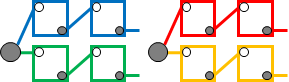
(a) Initial state

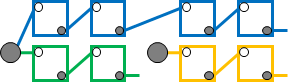
(b) One road extended

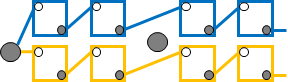
(c) Merge complete

Figure 5: Visualization of merging a pair of $2$-roads of length $d=2$ to a single twice longer $2$-road. In this example $k\geq 4$. Initially the $2$-roads are disjoint. Then, we cut a road from the right $2$-road and extend another road in the left $2$-road. If necessary, the algorithm recolors one or more of the roads. Then we do the same for the remaining road. In the end, the hub of the cut-down $2$-road is a node of degree $0$.

*

Proof.

This proof uses a similar high-level construction as the one used to prove Lemma 6.1, and the only difference is in the way we merge pairs of $r$-roads. Here we set $r=k$. Assume for now that when merging two $k$-roads of length $d$, $OPT$ pays $O(k\log k)$ and any algorithm pays $\Omega(k\log k\cdot d)$ in expectation.

With this in mind, revisit the competitive analysis: when a phase begins $OPT$ pays $O(2^{h}\cdot k\cdot d_{0})$ to recolor bricks to their desired color, it then pays $\sum_{i=1}^{h}{2^{h-i}\cdot O(k\log k)}=O(2^{h}\cdot k\log k)$ in the merging rounds, and finally it pays $O(2^{h}\cdot k\cdot d_{0})$ to restore the original $k$-roads for the next phase. Overall, its cost is $O(2^{h}\cdot k\cdot(d_{0}+\log k))$. In comparison, $ALG$ pays for recoloring, in expectation, at least $\sum_{i=1}^{h}{2^{h-i}\cdot\Omega(k\log k\cdot 2^{i-1}\cdot d_{0})}=\Omega(h\cdot 2^{h}\cdot k\log k\cdot d_{0})$. Assuming a sequence with $t=\Omega(k^{2})$ phases, we get that the competitive ratio is $\frac{\mathbb{E}[cost(ALG)]}{cost(OPT)}=\Omega(\frac{h\cdot 2^{h}\cdot k\log k\cdot d_{0}}{2^{h}\cdot k\cdot(d_{0}+\log k)})=\Omega(\frac{h\cdot\log k\cdot d_{0}}{d_{0}+\log k})$. To maximize the expression we balance and choose $d_{0}=\lceil\log k\rceil$, getting $\Omega(h\log k)$. We determine $h$ as before, except that the complicated merging technique requires a reusable extra node, so we have that $h\geq\lfloor\log\frac{n-1}{4k^{2}\cdot d_{0}+1}\rfloor$. Simplified, and with $d_{0}=\lceil\log k\rceil$, we get $h=\Omega(\log\frac{n}{k^{2}\log k})$, therefore the competitive ratio is $\Omega(\log\frac{n}{k^{2}\log k}\cdot\log k)$.

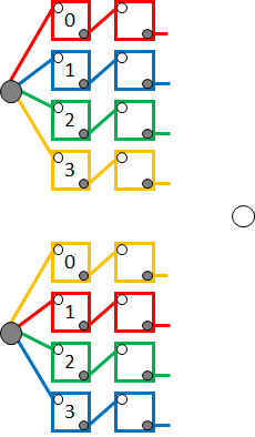
(a) Initial state

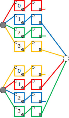
(b) Step 1

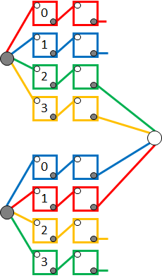
(c) Step 2

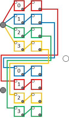
(d) Final merge

Figure 6: Visualization of merging a pair of $k$-roads, for $k=4$, of length $d=2$ to a single twice longer $k$-road, by “negative information”. (a) The roads are numbered from $0$ to $3$, with their number written inside their first brick. There are $\log k=2$ steps. (b) In the first step we temporarily connect roads $\{1,3\}$ (least significant bit $1$) of the top $k$-road with either roads $\{0,2\}$ or $\{1,3\}$ of the bottom $k$-road, to a shared hub (the white node). In this example we connect $\{1,3\}$, and as a results roads $2$ and $3$ of the bottom $k$-road were recolored. (c) In the second step we temporarily connect roads $\{2,3\}$ (second bit is $1$) of the top $k$-road with either roads $\{0,1\}$ or $\{2,3\}$ of the bottom $k$-road to a shared hub. In this example we connect $\{0,1\}$, and as a result roads $0$ and $2$ of the bottom $k$-road were recolored. (d) Finally there is a round of “positive information” in which we simply extend each road on the top color-consistently with a road on the bottom. The consistency depends on the choices of the previous steps, and in this example it matches road $x$ on the top with road $x\oplus 1$ on the bottom. The recoloring in this example is such that in the final extension no road is recolored.

Now we explain and analyze in details the merging of two $k$-roads, denote them by $X$ and $Y$. See Figure 6 for a visual example with $k=4$. For simplicity, let us start with $k$ being an integer power of $2$, say $k=2^{\ell}$. We start with $\ell$ steps of “negative information” in which we reveal roads that are of different colors, and do so by connecting the free end of these roads to a new shared hub, denote it by $v$. Concretely, number the roads of $X$ from $0$ to $k-1=2^{\ell}-1$ and denote by $X_{i,b}$ the roads of $X$ whose $i$th bit is $b$. We define similarly the subsets of roads for $Y$. In round $i$, we connect to $v$ the roads $X_{i,1}$ and $Y_{i,b_{i}}$ where $b_{i}$ is chosen uniformly at random between $0$ and $1$. Note that $|X_{i,1}|=|Y_{i,b_{i}}|=\frac{k}{2}$ so the degree of $v$ is $k$ (legal). When the round ends, we delete the edges of $v$. Finally, in the $\ell+1$ step we produce the longer $k$-road with “positive information” by cutting the roads of $Y$ from their hub and extending the roads of $X$, according to the unique way which does not contradict the previous $\ell$ steps. This way exists: road $y\in Y$ extends the road $x$ whose binary representation is $x=y\oplus B$ where the bits of $B$ are $b_{i}$ and $\oplus$ is the bitwise exclusive-or operation.

Let us analyze the costs of $OPT$ and $ALG$. Since $OPT$ knows the correct colors in advance, it can pay at most $1$ per edge that is inserted. We insert $k$ edges per step (even if most of them are later deleted), in a total of $\ell+1$ steps. This totals to $O(k\log k)$. We argue that $ALG$ recolors in expectation $\Omega(k)$ roads per each of the first $\ell$ steps. To simplify the analysis, assume that $ALG$ recolors after learning $b_{i}$ rather than being introduced online each edge of $v$ one by one (which can only hurt $ALG$). Then indeed every road in $X_{i,1}$ has probability $\frac{1}{2}$ to be in a conflict of color with a road of $Y_{i,b_{i}}$, so by the linearity of expectation, we get at least $\frac{k}{2}=\Omega(k)$ road recolorings (if $ALG$ is “reasonable”, it recolors $O(k)$ roads per step, so allowing it to be semi-offline did not lose more than a constant factor). Observe that our bound for round $i$ is not affected by previous rounds. So we conclude that $ALG$ pays $\Omega(\ell\cdot k\cdot d)=\Omega(k\log k\cdot d)$ for recoloring in expectation.

The case of $k$ not being a power of $2$ is similar. Each road is still assigned a number, and we regard its binary representation with $\lceil\log k\rceil$ bits, but only make $\ell=\lfloor\log k\rfloor$ rounds. Note that now $X_{i,1}$ is not necessarily of size $\frac{k}{2}$, but rather might be smaller. The bias is always in favor of $0$ because of how counting works, and it is such that $|X_{i,1}|\geq\frac{k-2^{i}}{2}$ ($i=0$ is the least significant bit). So we can still choose $Y_{i,b_{i}}$ with $b_{i}$ uniformly random, there is no problem to connect all the roads of $X_{i,1}$ and $Y_{i,b_{i}}$ to their shared hub. Also, each road in $X_{i,1}$ still has a color conflict with probability $\frac{1}{2}$. The only thing that changes is that the expectation of road recolorings is not $\frac{k}{2}$ per round, but rather $|X_{i,1}|$ in round $i$. This yields at least $\sum_{i=0}^{\ell-1}{|X_{i,1}|}\geq\ell\cdot\frac{k}{2}-\frac{1}{2}\sum_{i=0}^{\ell-1}{2^{i}}>\ell\cdot\frac{k}{2}-\frac{2^{\ell}}{2}>\frac{(\ell-1)k}{2}$ road recolorings in expectation for $ALG$, which is still $\Omega(k\log k)$ in total. The analysis of $OPT$ is unchanged, and its total cost is $O(k\log k)$ in total per merging a pair of $k$-roads (of any length). ∎

Remark 6.2.

A few notes on the proofs of Lemma 6.1 and Theorem 3.2:

1. The random choices of the adversary can be boiled-down to the random order of extending roads (in Lemma 6.1) and the bits $b_{i}$ (in Theorem 3.2). The $2$-roads and $k$-roads themselves are chosen once, and even the pairings of each merging round may be fixed.

2. For clarity, we presented it as if we need $2^{h}$ different hubs, one per $r$-road. In fact, we only need $h+1$ hubs if we reuse them: $h$ of them to maintain an $r$-road for each unique length, and another one for the length in which we currently merge a pair of $r$-roads. Of course, this saving is negligible compared to the number of nodes used to compose the roads.

6.3 Further Discussion on Randomization for Caching in Matchings

The gap between lower and upper bounds is not too wide in the deterministic case, when $k$ is small (e.g. $k=O(1)$), but it is exponentially wide with respect to $n$ in the randomized case. It is quite common that randomized algorithms achieve better competitive ratios, and it is particularly known in caching and other online problems (e.g., k-servers), which gives a “reason” to believe this may be so for Caching in Matchings as well.

In this section we describe a naive randomized algorithm and prove that it fails, and then proceed to discuss in details a more promising direction based on linear programming formulation.

Lemma 6.3.

Consider the following randomized algorithm, $ALG$: When a new edge is requested, if no matching can accommodate it, pick its color uniformly at random and evict conflicting neighbours. For $k=2$, $ALG$ is $\Omega(n)$ competitive.

Proof.

We construct a sequence on which the expected cost of this algorithm is high. The construction proceeds in alternating phases as follows. We single out a special node $u$ and divide the rest into $2L=\Theta(\frac{n}{k})=\Theta(n)$ (since $k=2$) bricks, from which we construct two roads of length $L$ each. See Figure 7:

1. In odd phases we regard $u$ and the two roads as a $2$-road. That is, we add the two edges that connect $u$ to the roads.

2. In even phases we regard the two roads as a single long road. That is, we add an extra edge that connects between the last brick of the first road and the first brick of the second road.

Every phase has $m$ rounds, and in each round we request all the edges of the structure of that phase (the $2$-road or single long road), in some arbitrary order.

By definition, in order to fully transition from one structure to the other, at least one road (of length $L$) must be recolored, because in odd phases they should disagree in color, and in even phases they should agree in color. As an upper bound for $OPT$, consider an algorithm that simply recolors one of the roads when a new phase begins, then $OPT$ pays $O(L)$ per phase. Next, consider $ALG$ on an odd-then-even pair of phases. In general, we say that $ALG$ is stable in a phase if it caches all the edges of that phase simultaneously. When $ALG$ is unstable, at least one edge is missing from its cache. There are two cases:

1. $ALG$ is unstable by the end of the odd phase: If at some point during that phase $ALG$ was stable, it remains stable. Therefore we conclude that throughout the whole phase it was unstable, and paid at least $1$ per round. In total, $ALG$ pays for the two phases at least $m$ (due to the odd phase).

2. $ALG$ is stable by the end of the odd phase: then the two roads have different colors and $ALG$ is unstable with respect to the new even phase. $ALG$ pays at least $1$ per round until either it stabilizes or the phase ends. Observe that since $k=2$, a brick is simply a path of three edges, and that the graph is simply a path of $8L-1$ edges whose red/blue “parity” is mismatched in the middle. We can order the path as a line, and correspond the edges to integers. When the missing edge, the hole, is requested, choosing its color is equivalent to randomly moving the hole left or right. So $ALG$ stabilizes in the even phase if and only if the corresponding random walk reaches $4L-1$ or $-(4L-1)$ (starting from $0$, the middle), see Figure 8. It is known that the expected number of steps in such a random walk to reach either $a$ or $-b$ ($a,b>0$) is $a\cdot b$. Therefore if $m$ was infinite, $ALG$ would pay in expectation $\Omega(L^{2})$. Because $m$ is finite, the expectation is smaller. However, Lemma 6.4 proves that by choosing $m$ to be large enough, say $N$, the truncation loses at most a constant factor, and still yield an expected cost of $\Omega(L^{2})$.

By choosing $m=\max\{N,L^{2}\}$ we get that $ALG$ pays in expectation $\Omega(L^{2})$ for the pair of phases in either case. A repetition of enough phases makes the initialization cost (pre-phases) negligible, and yields a competitive ratio $\Omega(L)=\Omega(\frac{n}{k})=\Omega(n)$ (recall that $k=2$). ∎

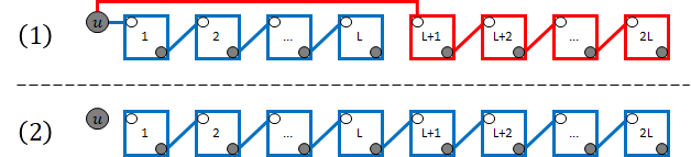
Figure 7: The two states of graph in Lemma 6.3. (1) During odd phases, requested edges imply a $2$-road. (2) During even phases, requested edges imply a single long road.

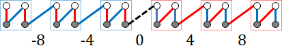
Figure 8: The initial state of an unstable even phase induces a random walk on the integer line. The left (blue) road and the right (red) road form a path of edges with a “hole” marked by the dashed black edge whose location changes according to a random walk. For clarity we only marked some of the integers, those that correspond to edges between bricks.

It is plausible that Lemma 6.3 should generalize to a lower bound of $\Omega(\frac{n}{k})$ for $k\geq 2$. The proof should go almost exactly the same, except that now the random walk argument is not trivial. When $k>2$, a road is not simply a path, and there are two issues: (1) When randomly coloring an added edge, it is possible that two neighbouring edges would be removed, creating multiple holes that may help or interfere with the movement of other holes; (2) The random walk itself is not as clean as a walk on the integer line. There are still “bottlenecks” thanks to the edges between consecutive bricks, but one should be careful when analyzing the probabilities to advance a hole towards the ends of the roads. Moreover, even if everything is symmetric at the beginning of the even phase, after $ALG$ starts recoloring edges, it gets messier because different bricks may have different coloring to their “inside edges”, affecting the probability of a hole crossing over each brick.

Lemma 6.4.

Consider a random walk that starts at $0$, moving at each step to either side with probability $\frac{1}{2}$ each. Let $E_{m}$ be the expected number of steps until stopping, either due to reaching $a>0$ or $-b<0$, or after $m$ steps. Then there is $N>0$ such that for $m\geq N$, $E_{m}\geq\frac{1}{2}E_{\infty}$.

Proof.

Stopping the walk due to capping the number of steps only decreases the expectation, therefore $E_{1}\leq E_{2}\leq\ldots\leq E_{\infty}$. Let $p_{i}$ and $q_{i}$ be the probabilities that a non-truncated walk ends after exactly $i$ steps, and after more than $i$ steps, respectively ($p_{i+1}\leq q_{i}$). Note that if a block of consecutive $a+b$ steps walks to the right, then we stop (must hit $a$), so for every block of $a+b$ consecutive steps the probability to end the walk is at least $\frac{1}{2^{a+b}}$. Therefore $i$ steps can be divided to disjoint blocks of consecutive steps, and we conclude that $p_{i+1}\leq q_{i}\leq(1-\frac{1}{2^{a+b}})^{\lfloor i/(a+b)\rfloor}$. To simplify, denote $z=(1-\frac{1}{2^{a+b}})$ and remember that $z<1$. The exponential decrease of $q_{i}$ also implies that $E_{\infty}$ is bounded and well-defined, even without knowing its exact value ($E_{\infty}=a\cdot b$). Now:

$$E_{\infty}-E_{N}=\sum_{i=1}^{\infty}{i\cdot p_{i}}-\sum_{i=1}^{\infty}{\min\{i,N\}\cdot p_{i}}=\sum_{i=N+1}^{\infty}{(i-N)\cdot p_{i}}=\sum_{i=N}^{\infty}{(i+1-N)\cdot p_{i+1}}$$

Note that $i-(a+b)<(a+b)\cdot\lfloor i/(a+b)\rfloor$. Set $N=1+(c+1)\cdot(a+b)$ for integer $c\geq 1$ (to be determined), then $i+1-N\leq(a+b)\cdot(\lfloor i/(a+b)\rfloor-c)$. We continue:

$$\leq\sum_{i=N}^{\infty}{(i+1-N)\cdot z^{\lfloor i/(a+b)\rfloor}}\leq(a+b)\sum_{i=N}^{\infty}{(\lfloor i/(a+b)\rfloor-c)\cdot z^{\lfloor i/(a+b)\rfloor}}$$

We can batch all the summands for $j\cdot(a+b)\leq i\leq(j+1)\cdot(a+b)-1$ together. Continue by batching, and note that the first batch is incomplete (hence the strict inequality):

$$<{(a+b)}^{2}\sum_{j=c+1}^{\infty}{(j-c)\cdot z^{j}}=(a+b)^{2}z^{c}\sum_{j=1}^{\infty}{j\cdot z^{j}}=(a+b)^{2}z^{c}\cdot\frac{z}{(1-z)^{2}}$$

Since $\lim_{c\to\infty}{(E_{\infty}-E_{N})}=0$, choosing a large enough $c$ yields $N$ such that $E_{m}\geq\frac{1}{2}E_{\infty}$ for any $m\geq N$. ∎

Linear-formulation and rounding schemes: We can formalize the Caching in Matchings problem as a set of linear constraints, some of them arrive online and correspond to requests. This enables us to use additional tools and techniques for designing competitive algorithms [18], in particular for caching [2, 7]. The LP-formulation of our problem for a sequence $\sigma$ is given below.

$\min\sum_{t=1}^{|\sigma|}{\sum_{c=1}^{k}{\sum_{e\in E}{\Delta^{t}_{e,c}}}}$

Such that:

1. $\forall t:\sum_{c=1}^{k}{x^{t}_{\sigma(t),c}}\geq 1$ // Covering requested edges

2. $\forall t,v,c:\sum_{e\in E(v)}{x^{t}_{e,c}}\leq 1$ // Packing proper coloring, $E(v)$ are the edges of $v$

3. $\forall t,e,c:x^{t}_{e,c}-x^{t-1}_{e,c}\leq\Delta^{t}_{e,c}$ // Technical for the formulation

4. $\forall t,e,c:\Delta^{t}_{e,c},x^{t}_{e,c}\geq 0$ // Non-negativity

Fractional Caching in Matchings (Linear Program)

In simple words, the LP-formulation of the problem consists of $\Theta(n^{2}k)$ variables of the form $x_{e,c}$, one for every possible color of every possible edge. Technically, for defining the objective function of the LP, we define a different copy of each variable for each time, and also add the variables $\Delta^{t}_{e,c}$ to represent the growth of variable $x_{e,c}$ from time $t-1$ to time $t$. Note that the formulation only considers growth, which is fine because growth corresponds to fetching into the cache (i.e., if $x^{t}_{e,c}-x^{t-1}_{e,c}<0$ then the solution can have $\Delta^{t}_{c,e}=0$). We denote by $\sigma(t)$ the request at time $t$, the covering constraints ensure that at any time the current request is fully cached, and the packing constraints correspond to (fractional) proper coloring. We refer to this formulation as fractional Caching in Matchings. This is a special case of the online convex body-chasing problem, in the $L_{1}$ metric. Of course, the integer formulation requires to change the non-negativity constraints to $\forall t,e,c:x^{t}_{e,c}\in\{0,1\}$. While we can also add the constraints that $\forall t,e,c:x^{t}_{e,c}\leq 1$, these are implied, and a reasonable algorithm should never increase a variables to more than $1$. Indeed, increasing variables has a cost, a covering constraint that is satisfied by $x^{t}_{e,c}>1$ remains satisfied if $x^{t}_{e,c}=1$, and packing constraints loosen and also remain satisfied for smaller values. To simplify notations, henceforth we omit the time superscript from $x_{e,c}$.

In terms of body-chasing, the dimension of our problem is $d=\Theta(k\cdot n^{2})$ because there are $k$ colors and $\Theta(n^{2})$ edges. While an $\Omega(\sqrt{d})$ lower bound on the competitive ratio of randomized algorithms is known for general convex body-chasing [16, see Lemma 5.4], that bound necessitates an adversary that is much stronger than the adversary in our case. In our case, the adversary can only introduce a single temporary covering constraint at a time, while the rest of the constraints are fixed. Therefore, this lower bound cannot be used to argue for an $\Omega(\sqrt{k}\cdot n)$ randomized lower bound for Caching in Matchings.

If the packing constraints are relaxed such that $\sum_{e\in E(v)}{x_{e,c}}\leq 1+\epsilon$, we can use a more general result on convex body-chasing in $L_{1}$ of Bhattacharya et al. [11] that applies to our case.

Theorem 6.5 (Theorem 1.1 in [11]).

For any $\epsilon\in(0,1]$, there is an $O(\frac{1}{\epsilon}\cdot\log\frac{k}{\epsilon})$ competitive algorithm for fractional Caching in Matchings where the bound for each packing constraint is $1+\epsilon$ instead of $1$.

Unfortunately, Theorem 6.5 does not allow for $\epsilon=0$. One can think of $\epsilon>0$ as a kind of resource augmentation, but it is not the natural augmentation for our problem. Rather than having extra colors, this augmentation allows having a bit extra from each existing color. It does not seem that the two types of augmentations, having more colors and having more of the same colors, are equivalent.

At a first glance, it looks like we can remove the need for some of the augmentation.

Lemma 6.6.

Let $A$ be the algorithm claimed by Theorem 6.5 for $\epsilon=\frac{1}{2k}$. It satisfies $\forall v:\sum_{c=1}^{k}{\sum_{e\in E(v)}{x_{e,c}}}\leq k\cdot(1+\epsilon)$. We can transform it into an algorithm $B$ that guarantees:

1. $B$ satisfies the same constraints that $A$ does, the covering constraints, and the packing constraints up to $1+\epsilon$.

2. For any sequence of requests $\sigma$, $cost(B(\sigma))\leq 2\cdot cost(A(\sigma))$.

3. For every node $v$ at any time, $\sum_{c=1}^{k}{\sum_{e\in E(v)}{x_{e,c}}}\leq k$.

Proof.

We define $B$ such that it maintains the two following invariants. Note that this does not uniquely define $B$, but any algorithm that satisfies these invariants work. First, for every variable $x_{e,c}$, $x^{B}_{e,c}\leq x^{A}_{e,c}$ (superscripts correspond to the algorithms). Second, denote the total load of an edge $e$ by $a_{e}=\sum_{c=1}^{k}{x^{A}_{e,c}}$ and $b_{e}=\sum_{c=1}^{k}{x^{B}_{e,c}}$, we maintain that for every edge $e$: $b_{e}=\max\{2\cdot a_{e}-1,0\}$. Note that $e$ is fully cached in $B$ if and only if it is fully cached in $A$. Now we prove the claims in the order that we stated them:

1. When edge $e_{t}$ is requested, $a_{e_{t}}=1$ therefore $b_{e_{t}}=1$ as well and the covering constraint is satisfied. In addition, since $x^{B}_{e,c}\leq x^{A}_{e,c}$ for every $e$ and $c$, $B$ satisfies all the packing constraints (up to $\epsilon$) because $A$ does.

2. When $A$ changes $a_{e}$ by $\epsilon$, $B$ changes $b_{e}$ in the same direction (increasing or decreasing) by at most $2\epsilon$ (could be less if $a_{e}$ decreases below $\frac{1}{2}$, because the decrease of $b_{e}$ stops at $0$).

3. Fix the node $v$ with edges $E(v)$. Let $X$ be the set of edges of $v$ for which $a_{e}\leq\frac{1}{2}$ and let $Y=E(v)\setminus X$. Denote also the slack $s_{a}$ such that $(k+\frac{1}{2})-\sum_{e\in X\cup Y}{a_{e}}=s_{a}$, for $s_{a}\geq 0$. We need to prove that $\sum_{e\in Y}{b_{e}}\leq k$ (note that $\sum_{e\in X}{b_{e}}=0$ by definition of $X$ and the second invariant). There are two cases:

   1. If $\sum_{e\in X}{a_{e}}+s_{a}\geq\frac{1}{2}$, then we are done because $\sum_{e\in Y}{b_{e}}\leq\sum_{e\in Y}{a_{e}}\leq(k+\frac{1}{2})-\frac{1}{2}=k$.

   2. If $\sum_{e\in X}{a_{e}}+s_{a}<\frac{1}{2}$, then $\sum_{e\in Y}{a_{e}}>k$. Because each summand is bounded by $1$, $|Y|\geq k+1$. Then: $\sum_{e\in Y}{b_{e}}=2\sum_{e\in Y}{a_{e}}-|Y|\leq 2(k+\frac{1}{2})-(k+1)\leq k$. ∎

Since we chose $\epsilon=\frac{1}{2k}$ in Lemma 6.6, by Theorem 6.5 both $A$ and $B$ are $O(k\log k)$ competitive. While $B$ is not using more than a total of $k$ colors per node, it is not free of resource augmentation. We did not address the packing constraints specifically, but rather globally per node, and therefore the state of $B$ still allows the portion of some color in some node to exceed $1$ up to $1+\frac{1}{2k}$.

Other than the issue of the non-natural resource augmentation, there is of course the question of finding a rounding scheme. In order to get a randomized solution, one must find a rounding scheme for the fractional solution. It would be nice if the solution could be done in two steps, first resolving the augmentation of either algorithm $A$ or $B$, and then finding a rounding scheme, but the previous paragraphs hint that perhaps such separation is not so simple if it even exists.

6.4 Miscellaneous Proofs

We begin by re-stating and proving the theorem that derives a connection caching algorithm out of a caching algorithm, by losing only a factor of $2$ in the competitive ratio. The explicit derivation is given in Algorithm 1. For completeness, we formally define the caching problem.

Problem 4 (Caching).

A sequence of page requests $p_{1},p_{2},\ldots$ is revealed one at a time. An algorithm maintains a cache of size $k$. When a page that is not in the cache is requested, the algorithm must bring it to the cache, possibly evicting another, and pays $1$. The algorithm may also bring additional pages to cache, and the cost of the algorithm is $1$ per added page.

Input: A sequence of connection requests $\sigma$, revealed one at a time.

Function Init(caching algorithm $A$):

       Set the cache $M=\emptyset$.

       $\forall u\in V$: Initialize an instance $A_{u}$ and denote its virtual cache by $M_{u}$.

Function Serve(request $(u,v)$):

       Regardless of whether $(u,v)\in M$, feed $(u,v)$ to $A_{u}$ and to $A_{v}$.

       If $A_{u}$ added $(u,b)$ (for any $b\in V$) and $(u,b)\in M_{b}$ then add $(u,b)$ to $M$. If $A_{u}$ evicted $(u,b)$ and $(u,b)\in M$, then evict it from $M$.

       Similarly, if $A_{v}$ added $(b,v)$ and $(b,v)\in M_{b}$ then add $(b,v)$ to $M$. If $A_{v}$ evicted $(b,v)$ and $(b,v)\in M$ then evict it from $M$.

      

Algorithm 1 Decoupling Connection Caching

*

Proof.

The idea of the proof is to charge the cost of the connection caching algorithm to the virtual local caching algorithms that run on each node, while maintaining the invariant that an edge (connection) $(a,b)$ is cached if and only if it is cached in both virtual caches of $a$ and $b$.

To simplify notation, denote $\rho=c(r,k)$, so that $A$ is a $\rho$-competitive caching algorithm with additive constant $\delta\geq 0$. Fix the sequence of requests $\sigma$ for connections. For a vertex $u\in V$, let $\sigma_{u}\subseteq\sigma$ consist of the requests for edges $(u,w)$ for some $w\in V$. Also, denote $cost(ALG(\sigma);\sigma_{u})$ the cost of a connection caching algorithm $ALG$ over the sequence $\sigma$ when we only consider costs due to requests in $\sigma_{u}$. Let $OPT$ be the optimal algorithm for serving $\sigma$. The cost of each request $(u,v)\in\sigma$ is counted both in $cost(OPT(\sigma);\sigma_{u})$ and $cost(OPT(\sigma);\sigma_{v})$, thus $\sum_{u\in V}{cost(OPT(\sigma);\sigma_{u})}=2\cdot cost(OPT(\sigma))$.

We define $B_{u}$ to be an offline connection caching algorithm that minimizes $cost(ALG(\sigma);\sigma_{u})$ over all algorithms $ALG$, therefore $cost(B_{u}(\sigma);\sigma_{u})\leq cost(OPT(\sigma);\sigma_{u})$. By our definitions we can think of $B_{u}$ as a caching algorithm in $u$ running over $\sigma_{u}$. To clarify, since $k\geq 2$, $B_{u}$ can reserve the first cache slot of any $v(\neq u)\in V$ for the connection $(v,u)$ while using the rest of the slots to serve requests of edges $(v,w)$ for $w\neq u$.

We charge the cost of the algorithm for connection caching, denote it by $A^{\prime}$, on every request $(u,v)$ to the virtual cost of either $A_{u}$ or $A_{v}$, depending on the state of the cache when $(u,v)$ arrives as follows. By virtual cost we refer to the cost that each of these instances “thinks” that it pays, when $A^{\prime}$ feeds it with $(u,v)$ in order to use its decisions. Concretely, if $A^{\prime}$ fetched an edge $(u,b)$ for some $v\neq b\in V$, then by the invariant both $A_{u}$ and $A_{b}$ have it cached, but previously $A_{u}$ did not have it cached (the state of $A_{b}$ did not change). So we can charge the cost of $A^{\prime}$ to the virtual cost of $A_{u}$. Similarly we can charge the fetching of an edge $(b,v)$ for $u\neq b\in V$ to the virtual cost of $A_{v}$. Finally, if $A^{\prime}$ fetched $(u,v)$, either $A_{u}$ or $A_{v}$ (or both) must have fetched it too, so we can charge that one. Overall, $cost(A^{\prime}(\sigma))\leq\sum_{u\in V}{cost(A_{u}(\sigma_{u}))}$. Since $A_{u}$ is $\rho$-competitive with additive term $\delta$ against $B_{u}$ when $B_{u}$ is viewed as a caching algorithm, we can wrap-up as follows.

$$cost(A^{\prime}(\sigma))\leq\sum_{u\in V}{cost(A_{u}(\sigma_{u}))}\leq\sum_{u\in V}{(\rho\cdot cost(B_{u}(\sigma);\sigma_{u})+\delta)}$$

$$\leq\rho\sum_{u\in V}{cost(OPT(\sigma);\sigma_{u})}+|V|\cdot\delta=2\rho\cdot cost(OPT(\sigma))+|V|\cdot\delta$$

Note that the $2$ in the multiplicative term originates from the two sides of a connection, and the additive term is due to each node contributing separately up to $\delta$. If $A$ is randomized, the same analysis can be repeated as follows:

$$\mathbb{E}[cost(A^{\prime}(\sigma))]\leq\mathbb{E}\Big{[}\sum_{u\in V}{cost(A_{u}(\sigma_{u}))}\Big{]}=\sum_{u\in V}{\mathbb{E}[cost(A_{u}(\sigma_{u}))]}\leq\sum_{u\in V}{(\rho\cdot cost(B_{u}(\sigma);\sigma_{u})+\delta)}$$

$$\leq\rho\sum_{u\in V}{cost(OPT(\sigma);\sigma_{u})}+|V|\cdot\delta=2\rho\cdot cost(OPT(\sigma))+|V|\cdot\delta$$

∎

Remark 6.7.

Theorem 3.3 and Algorithm 1 can be generalized to other caching variants, such as generalized caching (edges may have different sizes in cache, and different costs) and caching with rejections [23]. The argument remains the same: due to the invariant, the cost paid for a connection can be charged to the cost of (at least) one local-cache cost of the connection’s end-points.

Lemma 6.8.

The arboricity of the line-graph $L(G)$ of a bipartite graph $G$ with maximum degree $k$ is at most $k$.

Proof.

Adding nodes and edges to a graph can only increase its arboricity, so first we can add to $L(G)$ nodes and edges to get a $d$-regular graph where $d=2k-2$, denote it $L^{\prime}$. Then by [3] the arboricity of $L^{\prime}$ is $\lceil\frac{d+1}{2}\rceil=k$, hence the arboricity of $L(G)$ is at most $k$ (adding edges can only increase the arboricity). ∎

Lemma 6.9.

Consider Caching in Matchings on a general graph. For fixed $k\geq 2$, There is an $O(n^{2}k^{2})$ competitive deterministic algorithm.

Proof.

We essentially repeat the standard phases-based proof that is used to show that a standard caching algorithm with a cache of size $r$ is $r$-competitive. The difference is that our effective cache size is $r=\frac{nk}{2}$, and that in each request we may completely reorganize the cache at a cost of $O(r)$ instead of only paying $1$ to cache the new request.

We define an online algorithm that acts in phases as follows. Every phase begins with an empty cache. During a phase, when a request arrives, check if there is any coloring of the edges that fits the existing edges and the new one. If there is, the phase continues, change the matchings accordingly to fit all the edges together. If not, we evict all the edges from the matchings and start a new phase. There can be at most $r=\frac{nk}{2}$ edges in the matchings overall, so a phase contains at most $r$ unique edges. When the matchings have $i\leq r$ edges in total, the recoloring cost is at most $i$ plus $1$ to insert a new edge. Note that we do not always have to recolor all the edges, in particular the first $k$ edges always have room without recoloring. We get that, per phase: $cost(ALG)\leq r+\sum_{i=k+1}^{r}{i}<r+\frac{r(r+1)}{2}=\frac{r(r+3)}{2}$.

Next we argue that $OPT$ pays at least $1$ per phase, which yields the competitive ratio $\frac{cost(ALG)}{cost(OPT)}=O(n^{2}k^{2})$. Denote the subsequence of requests of phase $i$ by $\phi_{i}$ and its first request by $r_{i}$. Then $r_{1}$ incurs a cost because the cache is initially empty. For $i>1$, we claim that either $r_{i}$ or some request in $\phi_{i-1}\setminus\{r_{i-1}\}$ incurs a cost. To see why, denote by $q$ the edge requested by $r_{i}$. Note that $q$ was not requested during $\phi_{i-1}$ since by definition it started a new phase. Moreover, there is no configuration of the cache in which $q$ could be part of $\phi_{i-1}$ or else it would have been, because $ALG$ fully rearranges its cache to pack additional edges, if possible. So if $r_{i}$ does not incur a cost, then $q$ must have been cached by $OPT$ during all of $\phi_{i-1}$, particularly right after $r_{i-1}$ was served, and there must be some other edge $q^{\prime}$ requested during $\phi_{i-1}\setminus\{r_{i-1}\}$ that was not cached when requested. ∎

References

- [1] Anna Adamaszek, Artur Czumaj, Matthias Englert, and Harald Räcke. An -competitive algorithm for generalized caching. In SODA, pages 1681–1689. SIAM, 2012.
- [2] Anna Adamaszek, Artur Czumaj, Matthias Englert, and Harald Räcke. An -competitive algorithm for generalized caching. ACM Trans. Algorithms, 15(1), 2018.
- [3] Jin Akiyama and Takashi Hamada. The decompositions of line graphs, middle graphs and total graphs of complete graphs into forests. Discrete Mathematics, 26(3):203–208, 1979.
- [4] Susanne Albers. Generalized connection caching. In ACM SPAA, page 70–78, 2000.
- [5] Chen Avin, Chen Griner, Iosif Salem, and Stefan Schmid. An online matching model for self-adjusting ToR-to-ToR networks, 2020. arXiv:2006.11148.
- [6] Yossi Azar, Chay Machluf, Boaz Patt-Shamir, and Noam Touitou. Competitive vertex recoloring. Algorithmica, 85:2001–2027, 2023.
- [7] Nikhil Bansal, Niv Buchbinder, and Joseph (Seffi) Naor. Randomized competitive algorithms for generalized caching. In STOC, page 235–244, 2008.
- [8] Nikhil Bansal, Niv Buchbinder, and Joseph (Seffi) Naor. A primal-dual randomized algorithm for weighted paging. J. ACM, 59(4), 2012.
- [9] Luis Barba, Jean Cardinal, Matias Korman, Stefan Langerman, André Renssen, Marcel Roeloffzen, and Sander Verdonschot. Dynamic graph coloring. Algorithmica, 81(4):1319–1341, 2019.
- [10] Leonid Barenboim and Tzalik Maimon. Fully dynamic graph algorithms inspired by distributed computing: Deterministic maximal matching and edge coloring in sublinear update-time. ACM J. Exp. Algorithmics, 24:1–24, 2019.
- [11] Sayan Bhattacharya, Niv Buchbinder, Roie Levin, and Thatchaphol Saranurak. Chasing positive bodies, 2023. arXiv:2304.01889.
- [12] Sayan Bhattacharya, Deeparnab Chakrabarty, Monika Henzinger, and Danupon Nanongkai. Dynamic algorithms for graph coloring. In SODA, pages 1–20, 2018.
- [13] Sayan Bhattacharya, Fabrizio Grandoni, Janardhan Kulkarni, Quanquan C. Liu, and Shay Solomon. Fully dynamic (+1)-coloring in O(1) update time. ACM Trans. Algorithms, 18(2), 2022.
- [14] Marcin Bienkowski, David Fuchssteiner, Jan Marcinkowski, and Stefan Schmid. Online dynamic b-matching: With applications to reconfigurable datacenter networks. SIGMETRICS Perform. Eval. Rev., 48(3), 2021.
- [15] Allan Borodin and Ran El-Yaniv. Online Computation and Competitive Analysis. Cambridge University Press, 1998.
- [16] Sébastien Bubeck, Bo’az Klartag, Yin Tat Lee, Yuanzhi Li, and Mark Sellke. Chasing nested convex bodies nearly optimally. In SODA, pages 1496–1508, 2020.
- [17] Niv Buchbinder, Shahar Chen, and Joseph (Seffi) Naor. Competitive algorithms for restricted caching and matroid caching. In ESA, pages 209–221, 2014.
- [18] Niv Buchbinder and Joseph (Seffi) Naor. The Design of Competitive Online Algorithms via a Primal-Dual Approach. Now Foundations and Trends, 2009.
- [19] Aleksander B. G. Christiansen and Eva Rotenberg. Fully-Dynamic Arboricity Decompositions and Implicit Colouring. In ICALP, pages 42:1–42:20, 2022.
- [20] Edith Cohen, Haim Kaplan, and Uri Zwick. Connection caching under various models of communication. ACM SPAA, 2000.
- [21] Jack Edmonds. Maximum matching and a polyhedron with 0,1-vertices. Journal of Research of the National Bureau of Standards Section B Mathematics and Mathematical Physics, page 125, 1965.
- [22] Antoine El-Hayek, Kathrin Hanauer, and Monika Henzinger. On -matching and fully-dynamic maximum -edge coloring, 2023. arXiv:2310.01149.
- [23] Leah Epstein, Csanád Imreh, Asaf Levin, and Judit Nagy-György. Online file caching with rejection penalties. Algorithmica, 71(2):279–306, 2015.
- [24] Amos Fiat, Richard M Karp, Michael Luby, Lyle A McGeoch, Daniel D Sleator, and Neal E Young. Competitive paging algorithms. Journal of Algorithms, 12(4):685–699, 1991.
- [25] Amos Fiat, Manor Mendel, and Steven S. Seiden. Online companion caching. In ESA, pages 499–511, 2002.
- [26] Monia Ghobadi, Ratul Mahajan, Amar Phanishayee, Nikhil Devanur, Janardhan Kulkarni, Gireeja Ranade, Pierre-Alexandre Blanche, Houman Rastegarfar, Madeleine Glick, and Daniel Kilper. ProjecToR: Agile reconfigurable data center interconnect. In ACM SIGCOMM, page 216–229, 2016.
- [27] Monika Henzinger, Stefan Neumann, and Andreas Wiese. Explicit and implicit dynamic coloring of graphs with bounded arboricity, 2020. arXiv:2002.10142.
- [28] Monika Henzinger and Pan Peng. Constant-time dynamic ( + 1)-coloring. ACM Trans. Algorithms, 2022.
- [29] Ian Holyer. The NP-completeness of edge-coloring. SIAM Journal on Computing, 10(4):718–720, 1981.
- [30] Manas Jyoti Kashyop, N. S. Narayanaswamy, Meghana Nasre, and Sai Mohith Potluri. Trade-offs in dynamic coloring for bipartite and general graphs. Algorithmica, 85:854–878, 2023.
- [31] J. Misra and David Gries. A constructive proof of Vizing’s theorem. Information Processing Letters, 41(3):131–133, 1992.
- [32] Shay Solomon and Nicole Wein. Improved dynamic graph coloring. ACM Trans. Algorithms, 16(3):1–24, 2020.
- [33] Andrew Chi-Chin Yao. Probabilistic computations: Toward a unified measure of complexity. In SFCS, pages 222–227, 1977.
- [34] Neal Young. Competitive paging and dual-guided algorithms for weighted caching and match- ing. PhD thesis, Computer Science Dept., Princeton University, 1991.