Training Image Derivatives: Increased Accuracy and Universal Robustness

Abstract

Derivative training is a known method that significantly improves the accuracy of neural networks in some low-dimensional applications. In this paper, a similar improvement is obtained for an image analysis problem: reconstructing the vertices of a cube from its image. By training the derivatives with respect to the 6 degrees of freedom of the cube, we obtain 25 times more accurate results for noiseless inputs. The derivatives also offer insight into the robustness problem, which is currently understood in terms of two types of network vulnerabilities. The first type involves small perturbations that dramatically change the output, and the second type relates to substantial image changes that the network erroneously ignores. Defense against each is possible, but safeguarding against both while maintaining the accuracy defies conventional training methods. The first type is analyzed using the network’s gradient, while the second relies on human input evaluation, serving as an oracle substitute. For the task at hand, the nearest neighbor oracle can be defined and expanded into Taylor series using image derivatives. This allows for a robustness analysis that unifies both types of vulnerabilities and enables training where accuracy and universal robustness are limited only by network capacity.

1 Introduction

Neural networks are applied to a wide range of problems, and their use is justified by theorems [1, 2, 3] that guarantee the existence of parameters that achieve an arbitrarily accurate solution. Their most prominent use cases are high-dimensional approximations that require deep architectures [4]. For deep networks, the main tool for tuning parameters is gradient-based optimization, which minimizes the deviation of the network from the target function. However, the local nature of such methods prevents them from achieving arbitrarily low error even in simple cases [5]. In the previous paper [5] we showed that the accuracy of gradient-based training can be significantly improved if the deviations of the network derivatives from the target derivatives are also minimized. This method has been shown to work well for relatively low-dimensional applications such as differential equation solving [6], computational chemistry [7, 8], robotic control [9, 10], transport coefficients evaluation [11], and Bayesian inference [12]. Applications to high-dimensional problems such as image analysis have not yet been considered.

In high-dimensional cases, the notion of accuracy is somewhat different. The data usually belongs to a lower dimensional manifold [13, 14], and a small error on this set can be completely ruined by a small perturbation from the full input space. The issue of accuracy is therefore inextricably linked to the resilience to perturbations. This resilience is typically described in terms of the response to adversarial examples, i.e., inputs that have been altered specifically to fool neural networks. There are two main types of adversarial examples. The first exploits excessive sensitivity: the network’s output is flipped, even though the changes in the data are imperceptible [15]. The gradient of the network contains enough information about the local sensitivity [16] that it can be used to design these attacks, and train the network to withstand them [17, 18]. The second type of adversarials exploits invariance: the output of the network remains the same, despite the essential changes in the input [19, 20]. The “essentiality” can only be determined by an oracle, so the creation of such adversarials requires human evaluation [21], which is basically an oracle substitute. This complicates the analysis of network vulnerabilities as well as the defense against them, which is still an open problem. Although the relationship between accuracy and robustness is far from obvious [22, 23, 24, 25, 26], recent work has shown that high accuracy is compatible with robustness against sensitivity attacks [27, 28], but there is a trade-off with the ability to withstand invariance attacks [21, 29]. Several studies consider accuracy and different types of robustness as conflicting goals and propose Pareto optimization [30] and other types of trade-offs [31, 32, 33]. Since robust and accurate perception obviously exists, there must be a flaw in the training methods or in the problem formulation.

This paper presents a simple image analysis problem for which an oracle can be constructed. Using derivatives of the target, it can be expanded in a Taylor series, which allows a detailed robustness analysis that unifies sensitivity and invariance-based attacks. We show in detail how standard robust training fails, and construct universal robust learning based on training derivatives. In addition, we show that derivatives can be used to significantly improve the accuracy of the non-robust problem, extending the results of [5] to image-input neural networks.

Section 3 formulates the problem, demonstrates a standard non-robust solution, and provides a definition of the oracle. In Section 4, the first derivatives of the images are computed and used to improve the accuracy of the non-robust formulation. A first-order expansion of the oracle is then constructed. A unified analysis of robustness is performed, first-order universal robust learning is proposed, and the results are compared against the standard robust training. Section 5 has a similar structure, but deals with second-order derivatives. The remaining sections are self-explanatory.

2 Motivation

The pursuit of the image analysis problem that could benefit from training derivatives was the immediate result of the study [5]. In this paper, neural networks have been used to approximate known functions of 2 and 3 variables. By using derivatives of the target up to 5th order, gradient training with RProp [34] achieved up to 1000 times more accurate approximation. But for real-world problems, evaluating even the first derivatives of the target becomes an issue. While a binary classifier that produces a smooth output is a common thing, its derivatives cannot be computed from the training labels. A few derivatives with respect to a priori invariant transformations are known to be zero, but unfortunately relying on invariance alone does not allow to increase the accuracy even in the simplest cases. 3-dimensional tracking problems offer a compromise between meaningful formulation and easy computation of derivatives. We will consider the special case of determining the vector of degrees of freedom for a rigid body - a cube. Since knowing this vector allows the reconstruction of the image, the task is similar to that of an encoder.

3 Problem formulation

3.1 Notations

Images are treated as vectors of Euclidean space and are denoted by calligraphic letters. Images from the manifold are denoted by $\mathcal{I}$. Elements of the full image space with no restrictions on pixel values are denoted by $\mathcal{F}$. The scalar product is denoted by a dot $\mathcal{I}\cdot\mathcal{F}$ and the norm is $\left\|\mathcal{I}\right\|=\sqrt{\mathcal{I}\cdot\mathcal{I}}$. For other vectors, the index notation is used $\vec{r}\equiv r_{i}$. Whenever indices are repeated in a single term, summation is implied, for example in the scalar product

$$r_{i}s_{i}\equiv\sum_{i}r_{i}s_{i}$$

or in squared norm $r_{i}r_{i}=\left\|\vec{r}\right\|^{2}$. Terms with non-repeating indices are tensors of higher rank, e.g. the outer product of two 3D vectors $r_{i}s_{j}$ is a 3 by 3 matrix. The symbol $\delta_{ji}$ is the Kronecker delta

$$\delta_{ji}=\begin{cases}0&i\neq j\\ 1&i=j\end{cases}$$

3.2 Problem Formulation

Consider a cube $C$ and an algorithm that renders its image $\mathcal{I}\left(C\right)$. Since $C$ has 6 degrees of freedom, its images belong to a 6-dimensional manifold. Our goal will be to determine the coordinates of the cube’s vertices

$$C=\left(\begin{array}[]{ccc}x_{1}&\ldots&x_{8}\\ y_{1}&\ldots&y_{8}\\ z_{1}&\ldots&z_{8}\end{array}\right)$$

from its image. To avoid a small mathematical obstacle described in Subsection 4.1, we aim to train a neural network $N$ with 9 outputs to determine the coordinates of the first three vertices when presented with an image

$$N\left(\mathcal{I}\left(C\right)\right)=\left(x_{1},y_{1},z_{1},x_{2},y_{2},z_{2},x_{3},y_{3},z_{3}\right).$$

Since the vertices are ordered, the rest of them can easily be reconstructed. For brevity, we will use this 9-dimensional vector interchangeably with the cube $C$ itself, so the task is

$$N\left(\mathcal{I}\left(C\right)\right)=C.$$ (1)

The particular component of the target is referred to as $C_{i}$, $i\in\left[1,9\right]$. If the rendering algorithm breaks the symmetry of the cube, e.g. by coloring its sides with different shades of gray, and delivers a perspective image that allows to track the depth, the problem is well posed. A precise mathematical formulation for such an algorithm is as follows.

3.3 Image Generation

This subsection provides details on image generation. Two key features are the smooth dependence of pixel values on cube position and the presence of perspective. The resulting images are shown in Fig. 1, details on the training set in Subsection 3.4, and the results of the conventional training in Subsection 3.5.

3.3.1 Projection

The perspective image of a 3-dimensional object is formed by projecting its points onto the image plane of a camera. The result depends on the position, orientation and focal length of the camera. The projection $\left(u,v\right)$ of the point $\left(x,y,z\right)$ can be obtained by linear transformation of vectors in homogeneous coordinates [35]

$$\left(\begin{array}[]{c}u\\ v\\ 1\end{array}\right)=\mathbf{P}\left(\begin{array}[]{c}x\\ y\\ z\\ 1\end{array}\right).$$ (2)

The left-hand side implies that the values of $u$ and $v$ are obtained by dividing the first two components of the vector by its third component. The matrix is

$$\mathbf{P}=\left(\begin{array}[]{ccc}\mathsf{f}&0&\mathsf{c_{x}}\\ 0&\mathsf{f}&\mathsf{c_{y}}\\ 0&0&1\end{array}\right)\left(\begin{array}[]{cccc}R_{11}&R_{12}&R_{13}&t_{x}\\ R_{21}&R_{22}&R_{23}&t_{y}\\ R_{31}&R_{32}&R_{33}&t_{z}\end{array}\right).$$

By default, the image plane is aligned with the $\left(x,y\right)$ plane and the camera is pointing in the $z$-direction. The vector $\left(t_{x},t_{y},t_{z}\right)$ moves the center of the camera, $\mathsf{c_{x}}$ and $\mathsf{c_{y}}$ move the center of the image along the image plane. A 3 by 3 matrix $R_{ij}$ rotates the camera. After projection, six sides of the cube produce up to three visible quadrilaterals $Q$ in the $\left(u,v\right)$ plane

$$Q=\left\{\left(u_{1},v_{1}\right),\left(u_{2},v_{2}\right),\left(u_{3},v_{3}\right),\left(u_{4},v_{4}\right)\right\},$$ (3)

which are colored according to the corresponding cube faces with intensities from $1/6$ to $1$. The empty space is black. We have assigned color to each point of the image plane, and can now proceed with the rasterization.

3.3.2 Rasterization

41 by 41 images are created by covering $\left[-1,1\right]^{2}$ area of the $\left(u,v\right)$ plane with a uniform grid of step $0.05$

$$u,v\in\left\{-1,-0.95,\ldots,1\right\}.$$

However, we cannot simply assign each pixel the color of the corresponding point of the image plane. First of all, this would produce an unnatural-looking image with sharp and irregular edges. Second, the pixel values will not be smooth functions of the cube position. To solve both problems, we implement an anti-aliasing procedure. The pixel intensity $p\left(u,v\right)$ is defined as a convolution of the color function and the Gaussian kernel

$$p\left(u,v\right)=\frac{1}{\sigma\sqrt{2\pi}}\iint\text{color}\left(u^{\prime},v^{\prime}\right)e^{-\frac{\left(u-u^{\prime}\right)^{2}+\left(v-v^{\prime}\right)^{2}}{2\sigma^{2}}}du^{\prime}dv^{\prime}.$$ (4)

The color intensity is zero everywhere except for non-overlapping quadrilaterals, so this integral can be split

$$p\left(u,v\right)=\sum_{\text{visible }Q}p\left(u,v,Q\right),$$

where the contribution of a single quadrilateral is

$$p\left(u,v,Q\right) =\frac{\text{color}\left(Q\right)}{\sigma\sqrt{2\pi}}\underset{Q}{\iint}e^{-\frac{\left(u-u^{\prime}\right)^{2}+\left(v-v^{\prime}\right)^{2}}{2\sigma^{2}}}du^{\prime}dv^{\prime}\equiv$$

$$\equiv\text{color}\left(Q\right)\underset{Q}{\iint}K\left(u,v,u^{\prime},v^{\prime}\right)du^{\prime}dv^{\prime}.$$ (5)

The image is a set of pixel intensities

$$\mathcal{I}\left(C\right)\equiv\left\{p\left(u,v\right)\mid u,v\in\left\{-1,-0.95,\dots,1\right\}\right\}.$$

The convolution parameter $\sigma$ should balance image smoothness and effective resolution. Consider the image area $\left[-1,1\right]^{2}$ covered by alternating black and white stripes. The effective resolution is the maximum number of lines that the formula (4) can resolve with 50% contrast loss [36]

$$\frac{p_{\max}-p_{\min}}{p_{\max}+p_{\min}}=0.5.$$

We chose $\sigma=0.03$, which resolves 28 lines and produces reasonably smooth images (see Fig. 1). Network generalization over different $\sigma$ is essentially the issue of robustness, which will be discussed in Subsections 4.6 and 5.4.

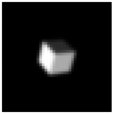
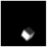
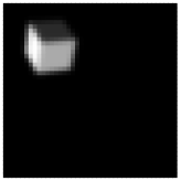
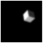
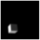
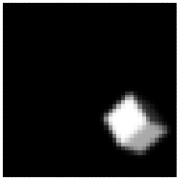
Figure 1: Images of the cube

3.4 Training Set

Before generating the training set, a few things should be considered. First of all, the range of cube positions should not place its projection outside of the image area. Second, the camera parameters and the size of the cube should produce a reasonable amount of perspective distortion. We choose $\mathsf{f}=5$, $t_{x}=t_{y}=0$, $t_{z}=-5$, no shift $\mathsf{c_{x}}=\mathsf{c_{y}}=0$ and no rotation $R_{ij}=\delta_{ij}$. The size of the cube is $2/5$ and the coordinates of its center vary in the range $\left[-0.52,0.52\right]$. This results in a visible width of 11 pixels at the closest position, 10 at the middle, and 9 at the farthest. To determine the range for rotations, we have to keep in mind that some symmetries are still present. As long as only one side is visible, the cube has 4 orientations that produce the same image. To avoid this ambiguity, the initial position of the cube has three equally visible sides

$$C_{0}=\frac{2}{5}\left(\begin{array}[]{ccc}\frac{-1}{\sqrt{6}}&0&\frac{-1}{\sqrt{6}}\\ \frac{-1}{\sqrt{2}}&0&\frac{1}{\sqrt{2}}\\ \frac{-1}{2\sqrt{3}}&\frac{\sqrt{3}}{2}&\frac{-1}{2\sqrt{3}}\end{array}\dots\right),$$

and its rotations along any axis $\vec{r}$ are limited to $\phi\in\left[-\frac{\pi}{8},\frac{\pi}{8}\right]$. Outputs are generated as

$$C\left(\vec{r},\phi,\vec{d}\,\right)=R\left(\vec{r},\phi\right)C_{0}+\vec{d},$$ (6)

where $R$ is the rotation matrix along the vector $\vec{r}$ at the angle $\phi$. The center of mass vector $\vec{d}$ is added to each column of the cube vertex matrix. $\vec{d}$ has three degrees of freedom, the unit vector $\vec{r}$ has two, and $\phi$ has one. The required 6 parameters are generated using Roberts’ version of the low discrepancy Korobov sequence [37]. They uniformly cover a 6-dimensional unit cube, as opposed to a random sequence that occasionally produces areas of higher and lower density. The first 4 components can be used for $\vec{d}$ and $\phi$ after a simple rescaling. The last two are adjusted to $\rho\in\left[-1,1\right]$, $\theta\in\left[0,\pi\right]$ and produce $\vec{r}$ as

$$\begin{cases}r_{x}=\sqrt{1-\rho^{2}}\cos\theta\\ r_{y}=\sqrt{1-\rho^{2}}\sin\theta\\ r_{z}=\rho\end{cases}$$

The intensities of the visible faces are $1$, $2/3$, and $1/6$. The training and test sets consist of 97020 and 20160 images respectively, examples are shown in Fig. 1. The cost function is

$$E_{0}=\frac{1}{n^{2}}\sum_{\begin{subarray}{c}\textrm{training}\\ \textrm{set}\end{subarray}}\left\|N-C\right\|^{2},$$ (7)

where the normalization factor $n=\text{avg}\left\|C\right\|$ will play a role if additional derivatives are trained. To estimate the results, we calculate the normalized root mean squared error, averaged over the output components

$$e=\frac{1}{9}\sum_{i=1}^{9}\frac{\text{rms}\left(N_{i}-C_{i}\right)}{D_{i}}.$$ (8)

Here $D_{i}$ are the standard deviations of each component, all roughly equal to $0.3$.

3.5 Results

Since convolutional neural networks are not a necessity for image analysis [38], we will use multilayer perceptrons to maintain continuity with previous work [5]. To estimate the impact of network capacity, we will train 4 fully connected neural networks with the following layer configuration

$$1681,L,L,L,128,9,$$

where $L=256$, $512$, $1024$, and $2048$. The total number of weights in millions is 0.6, 1.5, 4, and 12, respectively. All hidden layers have activation function

$$f\left(x\right)=\frac{1}{1+e^{-x}}.$$

The output layer is linear. The weights are initialized with random values from the range $\pm 2/\sqrt{\kappa}$, where $\kappa$ is the number of senders [39, 40]. For the first matrix, this range is increased to $\pm 10/\sqrt{1681}$ to compensate for the input distribution. Thresholds are initialized in the range $\left[-0.1,0.1\right]$. Training is done with ADAM [41] using the default parameters $\beta_{1}=0.9$, $\beta_{2}=0.999$, $\epsilon=10^{-8}$. The training set is divided into 42 batches, the number of epochs is 2000. The initial learning rate $l=10^{-3}$ is reduced to $l=10^{-4}$ for the last 50 epochs. Training was performed on Tesla A10 using tf32 mode for matrix multiplications.

TABLE I: Error in the initial problem (1) for conventionally trained networks

weights$\times$106		0.6	1.5	4	12
$e$,%	training	0.80	0.40	0.26	0.26
	test	1.04	0.60	0.43	0.45
time, minutes		1.5	3	6	16

Table I shows the results. The problem is not very demanding in terms of network capacity: the largest model is overfit and shows no improvement over the previous one. The number of iterations is also excessive, as the accuracy does not get much better after about 500 epochs. Larger networks and longer training will be more relevant in the following sections, here they are used for uniformity of results.

3.6 Adversarial Attacks

The cost function (7) for the problem (1) is defined only for images that belong to the 6-dimensional manifold of the 1681-dimensional input space. The full image space is mostly filled with noise, the output for which is of little concern. However, some of its elements are located close enough to the original data set to be visually indistinguishable, but the output of the network is drastically different [15]. As noted in [17], such images can be generated using the gradient of the network with respect to a given output. For the network with 12 million weights, the gradient with respect to the first output is shown in Fig. 2. Its norm is $0.71$. When added to the original image with a small factor

$$\mathcal{F}=\mathcal{I}\left(C\right)+\varepsilon\nabla N_{1},$$

the first output can be estimated as

$$N_{1}\left(\mathcal{F}\right)\simeq N_{1}\left(\mathcal{I}\left(C\right)\right)+\varepsilon\left\|\nabla N_{1}\right\|^{2},$$

the change is $\sim 0.5\varepsilon$, while each individual pixel is only altered by $\sim 0.03\varepsilon$. Even for $\varepsilon\sim 1$, this does not change the visual perception of the cube in the slightest. As a result, two nearly identical images have completely different outputs. This is commonly known as a sensitivity-based adversarial attack. All of the well-established properties of such attacks [17] hold true for the problem in question: they generalize well across different inputs, different network capacities, and different training methods. This apparent flaw gave rise to the notion of robustness as invariance to small perturbations [42]. Using the gradient as a tool to estimate the effect of perturbations, significant progress was made in training robust networks [16, 43]. However, another attack vector was later identified [19]. Even for networks certified to withstand perturbations up to a certain magnitude, it was possible to modify an image within that range so the output remained the same, but the essence of the image was changed [21]. This was called an invariance-based attack. Its source is not the response of the network, but rather the variability of the target (oracle). This discovery changed the definition of robustness to essentially matching the oracle, which makes quantitative analysis of vulnerabilities more difficult. Even the creation of invariance-based adversarials requires human evaluation [19, 20], which further complicates robust training. After an apparent trade-off between robustness against invariance and sensitivity attacks was reported [21, 29], several studies addressed them as conflicting goals [31, 33, 30].

The relative simplicity of the tracking problem (1) allows to us to construct a precise definition for the oracle and to investigate all aspects of robustness.

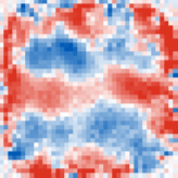
Figure 2: Gradient of the network with respect to its first output: $\nabla N_{1}$

3.7 Oracle

The oracle is a function that matches (1) on clean images and returns “the best possible output” for any other image $\mathcal{F}$. We will define it as the cube whose image is the closest in terms of Euclidean distance

$$\mathcal{O}\left(\mathcal{F}\right)=\arg\min_{C}\left\|\mathcal{I}\left(C\right)-\mathcal{F}\right\|^{2}.$$ (9)

For a generic point in the 1681-dimensional image space, this is a nonlinear 6-dimensional minimization problem. Solving it directly would require rendering a cube image for each iteration. If the image is close to the manifold $\mathcal{F}=\mathcal{I}+\varepsilon\mathcal{D}$, the expression (9) can be evaluated using a Taylor series

$$\mathcal{O}\left(\mathcal{I}+\varepsilon\mathcal{D}\right)=\mathcal{O}\left(\mathcal{I}\right)+\varepsilon\frac{\partial\mathcal{O}}{\partial\mathcal{D}}+\frac{\varepsilon^{2}}{2}\frac{\partial^{2}\mathcal{O}}{\partial\mathcal{D}^{2}}+o\left(\varepsilon^{2}\right).$$ (10)

Its terms can be computed using image derivatives with respect to the degrees of freedom of the cube. The robustness of the network can be evaluated using the expansion of

$$\left\|N\left(\mathcal{F}\right)-\mathcal{O}\left(\mathcal{F}\right)\right\|^{2}.$$ (11)

Since the image derivatives can also be used to improve the accuracy of the non-robust formulation (1), we will start there. The first- and second-order expansions of the oracle are considered in Subsections 4.4 and 5.3, respectively. The analysis of (11) is presented in Subsection 4.5.

4 First Order

This section describes how first-order derivatives can be used to improve the accuracy and robustness of neural networks. In 4.1, the accuracy improvement technique is explained and applied to the tracking problem. Subsection 4.2 covers the evaluation of image derivatives and 4.3 presents the results for the non-robust formulation. Further subsections deal with robustness. In 4.4 the first-order Taylor expansion of the oracle is obtained. Subsection 4.5 uses this expansion to perform a linear robustness analysis. In 4.6 we present a first-order robust learning and compare its results with those of Gaussian augmentation and Jacobian regularization.

4.1 Accuracy Improvement Technique

From the work [5] it follows that if input and output are generated by a set of continuous parameters, the accuracy can be improved by training the derivatives with respect to these parameters. In our case, the cube $C$ and thus its image are generated by $\vec{r}$, $\phi$ and $\vec{d}$. To increase the accuracy of

$$N\left(\mathcal{I}\left(C\right)\right)=C,$$ (12)

we should compute 6 derivatives of the input

$$\frac{\partial\mathcal{I}}{\partial r_{i}},\frac{\partial\mathcal{I}}{\partial\phi},\frac{\partial\mathcal{I}}{\partial d_{j}},$$

where $i=1,2$ and $j=1,2,3$. With an extended forward pass, we compute network derivatives

$$\mathcal{I},\frac{\partial\mathcal{I}}{\partial r_{i}},\frac{\partial\mathcal{I}}{\partial\phi},\frac{\partial\mathcal{I}}{\partial d_{j}}\overset{\begin{subarray}{c}\textrm{forward}\\ \textrm{pass}\end{subarray}}{\longrightarrow}N,\frac{\partial N}{\partial r_{i}},\frac{\partial N}{\partial\phi},\frac{\partial N}{\partial d_{j}},$$

which are then trained to match the derivatives of the target

$$C,\frac{\partial C}{\partial r_{i}},\frac{\partial C}{\partial\phi},\frac{\partial C}{\partial d_{j}},$$

as follows from the differentiation of the relation (12). However, our choice of rotation parameters interferes with this procedure. If $\phi=0$, the derivatives with respect to $r_{i}$ are zero, so 2 out of the 6 relations vanish. We could choose a different parameterization, but a similar problem will exist for any set of 3 global and continuous parameters that determine the orientation of a rigid body. It is caused by intrinsic properties of the rotational group [44]. There are several ways to get around this issue. For example, we could increase the number of parameters, as we did by choosing 9 output components for a problem with 6 degrees of freedom. A more resourceful approach is to use 6 parameters, but make them local. The reasoning is as follows. A cube image is a point on the 6-dimensional hypersurface. In a linear approximation, it is a plane defined by 6 independent tangent vectors. As long as we construct such vectors, the training data for that point is exhaustive: any other choice of parameters can only produce different (possibly degenerate) linear combinations of these vectors. Locality allows us to bind the definition of tangent vectors to the cube parameters, thus avoiding any issues.

4.1.1 Local Tangent Space

Consider a cube and its three rotations $R$ along the basis axes $x$, $y$ and $z$. Their combination $R_{z}\left(\nu_{3}\right)R_{y}\left(\nu_{2}\right)R_{x}\left(\nu_{1}\right)$ has a fixed point $\nu_{1}=\nu_{2}=\nu_{3}=0$, is smooth in its neighborhood and has 3 parameters with respect to which it can be differentiated. However, this operation will alter the center of mass vector if the cube is shifted from the origin. To isolate translations from rotations, we can move the cube to the origin, apply the composite rotation, and then move it back. The resulting transformation for a vertex $(x,y,z)$ is

$$R_{z}\left(\nu_{3}\right)R_{y}\left(\nu_{2}\right)R_{x}\left(\nu_{1}\right)\left(\begin{array}[]{c}x-d_{1}\\ y-d_{2}\\ z-d_{3}\end{array}\right)+ \left(\begin{array}[]{c}d_{1}+\nu_{4}\\ d_{2}+\nu_{5}\\ d_{3}+\nu_{6}\end{array}\right)\equiv$$ (13)

$$\equiv\hat{T}\left(\nu_{1},\nu_{2},\nu_{3},\nu_{4},\nu_{5},\nu_{6}\right)C$$

The second expression implies applying this transformation to each vertex of the cube. For brevity, we will use index notation for its arguments: $\hat{T}\left(\nu_{i}\right)$, $i\in\left[1,6\right]$. It is trivial to check that the operators $\partial\hat{T}/\partial\nu_{i}$ are linearly independent. They form 6 infinitesimal motions: three translations along $x$, $y$ and $z$ and three rotations about the same axes placed in the center of the cube. The derivatives of the images can be defined as

$$\frac{\partial\mathcal{I}}{\partial\nu_{i}}=\lim_{\varepsilon\rightarrow 0}\frac{\mathcal{I}\left(\hat{T}\left(\varepsilon\delta_{ij}\right)C\right)-\mathcal{I}\left(C\right)}{\varepsilon}.$$ (14)

Here $i$ is fixed, $\varepsilon\delta_{ji}$ is a compact notation for a vector $\nu_{j}$ whose $i$-th component is equal to $\varepsilon$ and the rest are 0. The simplest way to compute $\partial\mathcal{I}/\partial\nu_{i}$ is to rely on the precision of numerical integration (5) and evaluate the corresponding finite differences for sufficiently small $\varepsilon$. This works quite well for the first order, but becomes a bit time-consuming for the second derivatives. Our goal is to to obtain the explicit formulas for the first derivatives, which can then be used to evaluate higher derivatives via finite differences.

4.2 Image Derivatives

The coordinates of the cube vertex $\left(x,y,z\right)$ depend on the transformation parameters $\nu_{i}$. Their velocities

$$\frac{\partial\mathcal{C}}{\partial\nu_{i}}=\lim_{\varepsilon\rightarrow 0}\frac{\hat{T}\left(\varepsilon\delta_{ij}\right)C-C}{\varepsilon}$$ (15)

can be obtained directly by differentiating (13) with respect to $\nu_{i}$. The velocity of the image plane projection $\left(u,v\right)$ can be found from (2) by assuming $x=x\left(\nu_{i}\right)$, $y=y\left(\nu_{i}\right)$, $z=z\left(\nu_{i}\right)$ and taking derivatives with respect to $\nu_{i}$ at $\nu_{i}=0$. For the chosen camera parameters

$$\frac{\partial u}{\partial\nu_{i}}=\frac{\mathsf{f}}{t_{z}+z}\frac{\partial x}{\partial\nu_{i}}-\frac{\mathsf{f}x}{\left(t_{z}+z\right)^{2}}\frac{\partial z}{\partial\nu_{i}},$$

$$\frac{\partial v}{\partial\nu_{i}}=\frac{\mathsf{f}}{t_{z}+z}\frac{\partial y}{\partial\nu_{i}}-\frac{\mathsf{f}y}{\left(t_{z}+z\right)^{2}}\frac{\partial z}{\partial\nu_{i}}.$$

These are the velocities of the vertices of the quadrilaterals

$$\frac{\partial Q}{\partial\nu_{i}}\equiv\left\{\left(\frac{\partial u_{1}}{\partial\nu_{i}},\frac{\partial v_{1}}{\partial\nu_{i}}\right),\dots\right\},$$

and $Q$ determine the boundaries of the integration (5). The rate of change for integral (5) can be expressed as a line integral over the boundary

$$\frac{\partial p\left(u,v,Q\right)}{\partial\nu_{i}}=\text{color}\left(Q\right)\underset{\partial Q}{\oint}V_{n}\left(l\right)K\left(u,v,u^{\prime}\left(l\right),v^{\prime}\left(l\right)\right)dl,$$ (16)

where $V_{n}$ is the velocity of the boundary projected onto its outward normal. The integration is performed along 4 edges, which can be parameterized with $t\in\left[0,1\right]$. For the one between points 1 and 2

$$\begin{cases}u^{\prime}\left(t\right)=\left(1-t\right)u_{1}+tu_{2}\\ v^{\prime}\left(t\right)=\left(1-t\right)v_{1}+tv_{2}\end{cases}$$ (17)

The velocity of the boundary is a linear combination of the vertex velocities

$$\vec{V}\left(t\right)=\left(1-t\right)\left(\frac{\partial u_{1}}{\partial\nu_{i}},\frac{\partial v_{1}}{\partial\nu_{i}}\right)+t\left(\frac{\partial u_{2}}{\partial\nu_{i}},\frac{\partial v_{2}}{\partial\nu_{i}}\right)$$

and the normal vector is

$$\vec{n}=\frac{\left(v_{1}-v_{2},u_{2}-u_{1}\right)}{\sqrt{(v_{1}-v_{2})^{2}+(u_{2}-u_{1})^{2}}}.$$

The contribution to the integral (16) from this edge is

$$\int_{0}^{1}\left(\vec{V}\left(t\right),\vec{n}\right)K\left(u,v,u^{\prime}\left(t\right),v^{\prime}\left(t\right)\right)\frac{dl}{dt}dt,$$ (18)

where

$$\frac{dl}{dt}=\sqrt{(u_{2}-u_{1})^{2}+(v_{2}-v_{1})^{2}}.$$

The arguments of the Gaussian kernel $K\left(u,v,u^{\prime}\left(t\right),v^{\prime}\left(t\right)\right)$ are linear with respect to $t$, and $\left(\vec{V}\left(t\right),\vec{n}\right)$ is the first-order polynomial of $t$. This allows the integral (18) to be evaluated symbolically using the error function

$$\textrm{erf }x=\frac{2}{\sqrt{\pi}}\int_{0}^{x}e^{-t^{2}}dt.$$

For each $Q$ there are 4 integrals of the form (18). The derivative of the pixel intensity is the sum of the contributions from all visible quadrilaterals

$$\frac{\partial p\left(u,v\right)}{\partial\nu_{i}}=\sum_{\text{visible }Q}\frac{\partial p\left(u,v,Q\right)}{\partial\nu_{i}}.$$

The derivative of the image is

$$\frac{\partial\mathcal{I}}{\partial\nu_{i}}\equiv\left\{\frac{\partial p\left(u,v\right)}{\partial\nu_{i}}\mid u,v\in\left\{-1,-0.95,\dots,1\right\}\right\}.$$

Examples are shown in Fig. 3. By adding them to the original image, the cube can be moved within $\pm 0.04$ range in $x$ and $y$ directions, within $\pm 0.3$ in $z$ direction, and rotated up to 10 degrees about any axis. For larger transformations the linear approximation produces visible artifacts. In the neighborhood of any cube $\mathcal{C}$ we now have the first-order expansions

$$\mathcal{I}\left(\hat{T}\left(\nu_{i}\right)C\right)=\mathcal{I}\left(C\right)+\frac{\partial\mathcal{I}}{\partial\nu_{i}}\nu_{i}+o\left(\nu_{i}\right),$$ (19)

$$\hat{T}\left(\nu_{i}\right)C=C+\frac{\partial C}{\partial\nu_{i}}\nu_{i}+o\left(\nu_{i}\right).$$ (20)

The derivatives of $C$ are computed by differentiating (13) with respect to $\nu_{i}$ and substituting $\nu_{i}=0$.

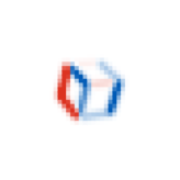
(a)

(b)

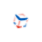
(c)

(d)

Figure 3: First-order image derivatives generated by infinitesimal operations: translations along the $x$ (a) and $z$ (b) axes and rotations about the $x$ (c) and $z$ (d) axes

4.3 Improving Accuracy

We can now use the derivatives to improve the accuracy of the original problem. The feedforward procedure receives an image and its derivatives, and calculates the output and corresponding derivatives of the network

$$\mathcal{I},\frac{\partial\mathcal{I}}{\partial\nu_{i}}\overset{\begin{subarray}{c}\textrm{forward}\\ \textrm{pass}\end{subarray}}{\longrightarrow}N,\frac{\partial N}{\partial\nu_{i}}.$$

The cost function (7) is augmented by the additional term

$$E_{1}=\sum_{\begin{subarray}{c}\textrm{training}\\ \textrm{set}\end{subarray}}\left[\sum_{i=1}^{6}\frac{1}{n_{i}^{2}}\left\|\frac{\partial N}{\partial\nu_{i}}-\frac{\partial C}{\partial\nu_{i}}\right\|^{2}\right],$$

the normalizing constant is the average norm of the corresponding output derivative, $n_{i}=\text{avg}\left\|\partial C/\partial\nu_{i}\right\|$. The gradient of the total cost $E=E_{0}+E_{1}$ is calculated using the extended backward pass. All training parameters are the same as in Subsection 3.5. The additional time needed for this training can be estimated by multiplying the times in the Table I by 6, which is the number of derivatives trained.

TABLE II: Error in the initial problem (1) for neural networks trained with first derivatives

weights$\times$106		0.6	1.5	4	12
$e$,%	training	0.16	0.11	0.067	0.065
	test	0.17	0.12	0.075	0.072

The results are shown in Table II. For all networks, the accuracy is increased about 5-6 times, which is close to the results obtained in [5] for 2-dimensional function approximation. Due to the excessive number of epochs, it is unlikely that the accuracy gap can be bridged, just as has been reported for the low-dimensional cases. The overfitting problem is almost resolved even for larger networks, similar to what was observed in [45]. The gradients with respect to the outputs are very similar to those produced by the regular training, which means that a perturbation with a norm of only $0.02$ can wipe out most of the improvements. This method would be more practical for networks with low-dimensional input and high-dimensional output, such as image generators. For image-input neural networks, a robust formulation is necessary.

4.4 Oracle Expansion

The robustness is determined by expression (11) and its linear analysis is most conveniently done by computing the gradients of $N$ and $\mathcal{O}$. While the gradient of the network can be computed efficiently using the backward pass, to find the gradient of the oracle, we need to compute the first directional derivative from the expression (10).

4.4.1 Derivatives

The first-order directional derivative is

$$\frac{\partial\mathcal{O}}{\partial\mathcal{D}}=\lim_{\varepsilon\rightarrow 0}\frac{\mathcal{O}\left(\mathcal{I}\left(C\right)+\varepsilon\mathcal{D}\right)-\mathcal{O}\left(\mathcal{I}\left(C\right)\right)}{\varepsilon}.$$ (21)

We have to figure out the term $\mathcal{O}\left(\mathcal{I}\left(C\right)+\varepsilon\mathcal{D}\right)$. Since any output of the oracle is a cube, the answer can be written as the transformation of the initial one

$$\mathcal{O}\left(\mathcal{I}\left(C\right)+\varepsilon\mathcal{D}\right)=\hat{T}\left(\nu_{i}\left(\varepsilon\right)\right)C,$$ (22)

where $\nu_{i}\left(\varepsilon\right)$ are unknown functions, $\nu_{i}\left(0\right)=0$. Substituting $\mathcal{F}=\mathcal{I}\left(C\right)+\varepsilon\mathcal{D}$ into the oracle definition (9), we get a minimization problem for $\nu_{i}\left(\varepsilon\right)$

$$\min_{\nu_{i}\left(\varepsilon\right)}\left\|\mathcal{I}\left(\hat{T}\left(\nu_{i}\left(\varepsilon\right)\right)C\right)-\mathcal{I}\left(\mathcal{C}\right)-\varepsilon\mathcal{D}\right\|^{2}.$$

It can be solved using Taylor expansion

$$\nu_{i}\left(\varepsilon\right)=\varepsilon\frac{d\nu_{i}}{d\varepsilon}+o\left(\varepsilon\right),$$

by plugging it into the first-order expansion of images (19), we obtain a minimization problem for $d\nu_{i}/d\varepsilon$

$$\min_{d\nu_{i}/d\varepsilon}\left\|\frac{\partial\mathcal{I}}{\partial\nu_{i}}\frac{d\nu_{i}}{d\varepsilon}-\mathcal{D}\right\|^{2}.$$

After expanding the squared norm and taking derivatives with respect to $d\nu_{j}/d\varepsilon$, we get

$$\underbrace{\left(\frac{\partial\mathcal{I}}{\partial\nu_{i}}\cdot\frac{\partial\mathcal{I}}{\partial\nu_{j}}\right)}_{\Gamma_{ij}}\frac{d\nu_{i}}{d\varepsilon}-\frac{\partial\mathcal{I}}{\partial\nu_{j}}\cdot\mathcal{D}=0.$$

The expression in parentheses is the Gram matrix for tangent vectors. Thus, we have a linear system of 6 equations

$$\Gamma_{ij}\frac{d\nu_{i}}{d\varepsilon}=\mathcal{D}\cdot\frac{\partial\mathcal{I}}{\partial\nu_{j}},$$ (23)

which can be solved by computing $\Gamma^{-1}$, which exists if the vectors $\partial\mathcal{I}/\partial\nu_{j}$ are linearly independent, which is true for any non-special point of the 6-dimensional hypersurface. The output of the oracle is

$$\mathcal{O}\left(\mathcal{I}\left(C\right)+\varepsilon\mathcal{D}\right)=C+\varepsilon\frac{\partial C}{\partial\nu_{i}}\frac{d\nu_{i}}{d\varepsilon},$$

and by plugging it into (21) we get the derivative

$$\frac{\partial\mathcal{O}}{\partial\mathcal{D}}=\frac{\partial C}{\partial\nu_{i}}\frac{d\nu_{i}}{d\varepsilon},$$

where $d\nu_{i}/d\varepsilon$ is the solution of (23).

4.4.2 Gradients

The gradients of the oracle are computed in two steps. First, we determine their direction, i.e., a normalized $\mathcal{D}$ for which a given output increases most rapidly. The magnitude of the gradient can then be found by evaluating the derivative of the oracle with respect to that direction.

For clarity, consider the output $\mathcal{O}_{1}$, which is $C_{1}$: the $x$-coodrinate of its first vertex in the cube. From (23) it follows that only the projection of $\mathcal{D}$ onto the tangent vectors $\partial\mathcal{I}/\partial\nu_{j}$ can contribute to $d\nu_{i}/d\varepsilon$ and thus to any change of $\mathcal{O}_{1}$. For this direction to an extremum, it must lie entirely in the 6-dimensional tangent space, and thus can be parameterized by a vector $\nu_{i}$

$$\mathcal{D}=\frac{\partial\mathcal{I}}{\partial\nu_{i}}\nu_{i}.$$ (24)

This simply means that the oracle has no adversarial inputs, instead any gradient will be a valid cube motion. In this case, the equation (23) has a simple solution $d\nu_{i}/d\varepsilon=\nu_{i}$, therefore

$$\mathcal{O}\left(\mathcal{I}\left(C\right)+\varepsilon\mathcal{D}\right)=C+\varepsilon\frac{\partial C}{\partial\nu_{i}}\nu_{i}.$$

The norm of $\mathcal{D}$ can be computed using the Gram matrix and we get a constrained maximization problem

$$\begin{cases}\max_{\nu_{i}}\dfrac{\partial C_{1}}{\partial\nu_{i}}\nu_{i}\\ \left\|\mathcal{D}\right\|^{2}=\Gamma_{ij}\nu_{i}\nu_{j}=1\end{cases}$$

After writing the Lagrangian and taking its partial derivatives, we get

$$\begin{cases}2\lambda\Gamma_{ij}\nu_{j}+\dfrac{\partial C_{1}}{\partial\nu_{i}}=0\\ \Gamma_{ij}\nu_{i}\nu_{j}=1.\end{cases}$$

We can use any $\lambda$ to find $\nu_{i}$ from the first equation, for example $\lambda=-1/2$

$$\Gamma_{ij}\nu_{j}=\dfrac{\partial C_{1}}{\partial\nu_{i}},$$ (25)

and then scale $\mathcal{D}$ to satisfy the constraint. Using the equation (25), the constraint can be simplified to

$$\frac{\partial C_{1}}{\partial\nu_{i}}\nu_{i}=1,$$

and the normalized gradient (24) is

$$\mathcal{D}=\frac{\frac{\partial\mathcal{I}}{\partial\nu_{i}}\nu_{i}}{\sqrt{\frac{\partial\mathcal{C}_{1}}{\partial\nu_{i}}\nu_{i}}}\equiv\frac{1}{\sqrt{g}}\frac{\partial\mathcal{I}}{\partial\nu_{i}}\nu_{i}.$$ (26)

The norm of the gradient is the magnitude of the directional derivative

$$\left\|\nabla\mathcal{O}_{1}\right\| =\frac{\partial\mathcal{O}_{1}}{\partial\mathcal{D}}=$$

$$=\lim_{\varepsilon\rightarrow 0}\frac{1}{\varepsilon}\left(\mathcal{O}_{1}\left(\mathcal{I}+\frac{\varepsilon}{\sqrt{g}}\frac{\partial\mathcal{I}}{\partial\nu_{i}}\nu_{i}\right)-\mathcal{O}_{1}\left(\mathcal{I}\right)\right)=$$

$$=\frac{1}{\sqrt{g}}\frac{\partial C_{1}}{\partial\nu_{i}}\nu_{i}=\sqrt{g}$$

which coincides with the initial norm of $\mathcal{D}$. The gradient of the oracle is thus

$$\nabla\mathcal{O}_{1}=\frac{\partial\mathcal{I}}{\partial\nu_{j}}\nu_{j},$$

where $\nu_{i}$ is the solution of (25). An example for $i=1$ is shown in Fig. 5a. Since all 9 gradients belong to the 6-dimensional tangent space, they are not linearly independent.

4.5 Robustness Analysis

Before we dive into optimal adversarial attacks, let us demonstrate a simple relationship. Consider the first component of the error $N_{1}-\mathcal{O}_{1}$ when the network and the oracle have unequal gradients $\nabla N_{1}\neq\nabla\mathcal{O}_{1}$. We can construct two directions

$$\mathcal{D}_{\text{inv.}}=\nabla\mathcal{O}_{1}-\left(\nabla N_{1}\cdot\nabla\mathcal{O}_{1}\right)\frac{\nabla N_{1}}{\left\|\nabla N_{1}\right\|^{2}}$$ (27)

$$\mathcal{D}_{\text{sen.}}=\nabla N_{1}-\left(\nabla N_{1}\cdot\nabla\mathcal{O}_{1}\right)\frac{\nabla\mathcal{O}_{1}}{\left\|\nabla\mathcal{O}_{1}\right\|^{2}}$$ (28)

$\mathcal{D}_{\text{inv.}}$ is perpendicular to $\nabla N_{1}$ but not to $\nabla\mathcal{O}_{1}$, so as we move along, in linear approximation the output $N_{1}$ does not change, but $\mathcal{O}_{1}$ does. It is thus a local equivalent of the invariance-based adversarial attack. The vector $\mathcal{D}_{\text{sen.}}$ represents sensitivity-based attack. If the network has no robust training, the term $\left(\nabla N_{1}\cdot\nabla\mathcal{O}_{1}\right)$ is usually negligible, and $\mathcal{D}_{\text{sen.}}$ is just an adversarial gradient. It is obvious that both attacks vanish simultaneously if $\nabla N_{1}=\nabla\mathcal{O}_{1}$, and there is no trade-off of any kind. Vulnerability to invariance and sensitivity-based attacks are two sides of the gradient misalignment.

4.5.1 Optimal Attack

We now seek to construct the optimal adversarial attack: a bounded perturbation that maximizes the error. This is a constrained maximization problem

$$\begin{cases}\max_{\mathcal{D}}\left\|N_{i}\left(\mathcal{I}+\varepsilon\mathcal{D}\right)-\mathcal{O}_{i}\left(\mathcal{I}+\varepsilon\mathcal{D}\right)\right\|^{2}\\ \left\|\mathcal{D}\right\|^{2}\leq 1\end{cases}$$ (29)

where $\varepsilon$ should be small enough for the first-order approximations to hold. If this is the case,

$$\begin{split}&N_{i}\left(\mathcal{I}+\varepsilon\mathcal{D}\right)-\mathcal{O}_{i}\left(\mathcal{I}+\varepsilon\mathcal{D}\right)=\\ =&\;N_{i}\left(\mathcal{I}\right)-\mathcal{O}_{i}\left(\mathcal{I}\right)+\varepsilon\mathcal{D}\cdot\nabla\left(N_{i}-\mathcal{O}_{i}\right).\end{split}$$ (30)

The situation where perturbation can significantly change the initial error is the one we are most interested in

$$\varepsilon\left\|\mathcal{D}\cdot\nabla\left(N_{i}-\mathcal{O}_{i}\right)\right\|\gg\left\|N_{i}\left(\mathcal{I}\right)-\mathcal{O}_{i}\left(\mathcal{I}\right)\right\|.$$ (31)

In this case, the problem is decoupled from $\varepsilon$ and the constraint can be replaced by the equality

$$\begin{cases}\max_{\mathcal{D}}\left\|\mathcal{D}\cdot\nabla\left(N_{i}-\mathcal{O}_{i}\right)\right\|^{2}\\ \left\|\mathcal{D}\right\|^{2}=1.\end{cases}$$ (32)

Here, $\mathcal{D}$ is a direction in which the deviation from the oracle increases most rapidly. As long as this maximum is large enough for (31) to hold with an acceptable $\varepsilon$, we do not need to consider the full expression (30). This simplification proved to be appropriate for all networks considered in this paper. The problem (29) would have to be considered if the interplay between the initial error and its increment cannot be ignored.

The magnitude of the maximum (32) can be used as a measure of the network’s vulnerability after appropriate normalization. Since the standard deviations of all outputs are about 0.3, a reasonable metric is

$$v=\frac{1}{0.3}\frac{\sqrt{\max}}{9}.$$ (33)

This value represents the rate at which the relative error increases, as we move along the optimal adversarial direction. For this type of attack, we will refer to it as $v_{\text{max}}$. The optimal direction is a linear combination of difference gradients

$$\mathcal{D}=\mu_{i}\nabla\left(N_{i}-\mathcal{O}_{i}\right).$$

After substituting this into (32) and denoting

$$G_{ij}=\nabla\left(N_{i}-\mathcal{O}_{i}\right)\cdot\nabla\left(N_{j}-\mathcal{O}_{j}\right),$$

we obtain a constrained maximization problem

$$\begin{cases}\max_{\mu}\left\|\mu_{i}G_{ij}\right\|^{2}\\ \mu_{i}\mu_{j}G_{ij}=1\end{cases}$$ (34)

whose solution is the eigenvector of $G_{ij}$ with the maximum eigenvalue

$$\mu_{i}G_{ij}=\lambda_{\max}\mu_{j},$$

$$\max_{\mu}\left\|\mu_{i}G_{ij}\right\|^{2}=\lambda_{\max}.$$

4.5.2 Invariance and Sensitivity-based Attacks

The construction of the optimal attacks using only invariance or sensitivity is a bit more nuanced. The optimal direction can be represented by a linear combination of gradients

$$\mathcal{D}=\nu_{i}\nabla\mathcal{O}_{i}+\omega_{i}\nabla N_{i}.$$ (35)

Since $i\in\left[1,9\right]$ this is formally an 18-dimensional problem, but only 6 of $\nabla\mathcal{O}_{i}$ are linearly independent, and the situation for $\nabla N_{i}$ is very similar. The behavior of $N$ is very well described in terms of the 6 largest eigenvectors of the matrix $\nabla N_{i}\cdot\nabla N_{j}$. For clean images, this is a consequence of having only 6 degrees of freedom, but it also holds very well for noisy and corrupted images. Denoting

$$\left(\begin{array}[]{cc}G_{ij}^{11}&G_{ij}^{12}\\ G_{ij}^{21}&G_{ij}^{22}\end{array}\right)=\left(\begin{array}[]{cc}\nabla\mathcal{O}_{i}\cdot\nabla\mathcal{O}_{j}&\nabla\mathcal{O}_{i}\cdot\nabla N_{j}\\ \nabla N_{i}\cdot\nabla\mathcal{O}_{j}&\nabla N_{i}\cdot\nabla N_{j}\end{array}\right)$$ (36)

and substituting (35) into (32) we get

$$\begin{cases}\max_{\nu,\omega}\left\|\nu_{i}\left(G_{ij}^{12}-G_{ij}^{11}\right)+\omega_{i}\left(G_{ij}^{22}-G_{ij}^{21}\right)\right\|^{2}\\ \nu_{i}\nu_{j}G_{ij}^{11}+\omega_{i}\omega_{j}G_{ij}^{22}+2\nu_{i}\omega_{j}G_{ij}^{12}=1\end{cases}$$ (37)

An additional constraint is needed to specify the type of the attack. If it is sensitivity-based, then $\mathcal{D}_{\text{sen.}}\cdot\nabla\mathcal{O}_{i}=0$, or

$$\nu_{i}G_{ij}^{11}+\omega_{i}G_{ij}^{21}=0.$$ (38)

This relation eliminates 2 out of the 4 terms in the expression to be maximized. Technically, this is 9 equations, while we expect 6. The extra can be removed by projecting (38) onto 6 eigenvectors of $G^{22}$ with largest eigenvalues. The constraint optimization problem for sensitivity-based perturbation is thus

$$\begin{cases}\max_{\nu,\omega}\left\|\nu_{i}G_{ij}^{12}+\omega_{i}G_{ij}^{22}\right\|^{2}\\ \nu_{i}\nu_{j}G_{ij}^{11}+\omega_{i}\omega_{j}G_{ij}^{22}+2\nu_{i}\omega_{j}G_{ij}^{12}=1\\ a_{kj}\left(\nu_{i}G_{ij}^{11}+\omega_{i}G_{ij}^{21}\right)=0\\ a_{ki}G_{ij}^{22}=\lambda_{k}a_{kj},\;k\in\left[1,6\right]\end{cases}$$ (39)

For a stacked vector $\left(\nu_{i},\omega_{i}\right)$ the first constraint is a quadratic form with matrix (36). The expression to be maximized a quadratic form as well. Given $P=G_{ij}^{12}$ and $W=G_{ij}^{22}$, its matrix is

$$\left(\begin{array}[]{cc}PP^{T}&PW^{T}\\ WP^{T}&WW^{T}\end{array}\right).$$ (40)

The solution method is as follows: first, we find a basis in which the matrix (36) becomes the identity. In this basis, we write a general solution for the second constraint as a linear combination of orthonormal vectors. We then use these vectors as a new basis in which we find the largest eigenvalue of the matrix (40), which is the desired maximum.

For the optimal invariance attack, the procedure is similar, only instead of (38) we have

$$\nu_{i}G_{ij}^{12}+\omega_{i}G_{ij}^{22}=0.$$

The system is

$$\begin{cases}\max_{\nu,\omega}\left\|\nu_{i}G_{ij}^{11}+\omega_{i}G_{ij}^{21}\right\|^{2}\\ \nu_{i}\nu_{j}G_{ij}^{11}+\omega_{i}\omega_{j}G_{ij}^{22}+2\nu_{i}\omega_{j}G_{ij}^{12}=1\\ a_{kj}\left(\nu_{i}G_{ij}^{12}+\omega_{i}G_{ij}^{22}\right)=0\\ a_{ki}G_{ij}^{11}=\lambda_{k}a_{kj},\;k\in\left[1,6\right]\end{cases}$$ (41)

The solution method is the same, except that the elements of (40) are now $P=G_{ij}^{11}$ and $W=G_{ij}^{21}$.

The vulnerabilities are quantified by substituting the values of the obtained maxima into the formula (33), and are denoted by $v_{\text{sen.}}$ and $v_{\text{inv.}}$. It is worth noting that if the gradient with respect to a certain output is much larger than others, the solutions of (39) and (41) are small corrections of the directions (28) and (27) for that output. We can now proceed to formulate a robust training algorithm.

4.6 Universal Robust Training

As linear theory suggests, the endpoint of robust training is a network whose gradients $\nabla N$ match the gradients of the oracle $\nabla\mathcal{O}$. Although there is a cheap way to compute $\nabla N$ after the backward pass, there is no easy way to train it. We could construct a computational graph that includes both forward and backward passes, but in this case, each weight would have a double contribution. This creates multiple paths and greatly increases the complexity of a potential backpropagation procedure for the new graph. This difficulty can be looked at from another angle. The condition on the gradient is equivalent to conditions on all derivatives with respect to inputs, since each of them can be computed using the gradient. Conversely, if a derivative with respect to a single pixel has the wrong value, the gradient will reflect that. We expect the gradient alignment problem to be on par with training all 1681 derivatives for all input patterns. Therefore, from the very beginning of the training, we aim to minimize

$$\left\|\frac{\partial N}{\partial\mathcal{D}}-\frac{\partial\mathcal{O}}{\partial\mathcal{D}}\right\|^{2}$$ (42)

for any clean image and any $\left\|\mathcal{D}\right\|=1$.

4.6.1 Random Directions

To approach this task, we will use the idea from the previous article [6]. There it was shown that training derivatives with respect to a few random directions for each point is a good substitute for minimizing all possible derivatives. However, this method allows to reduce the number of derivatives only a few times. To reach the order of thousands, we will randomize the directions after each epoch, essentially offloading the number of directions per pattern onto the number of epochs. This will be the main reason for the increase in the number of iterations compared to the original problem.

The minimal goal is to obtain a low error for perturbations such as the adversarial gradient shown in Fig. 2. Using them as directions is ineffective because they generalize to well across training samples: the average scalar product of two normalized gradients is about 0.7. We want to create a family of directions that look similar but actually independent from each other. As a building block, we use the convolution of white noise with a Gaussian matrix

$$G_{ij}\left(r\right)=\frac{1}{N}\exp\left(\frac{-2}{r^{2}}\left[\left(i-r-1\right)^{2}+\left(j-r-1\right)^{2}\right]\right)$$

where $i,j\in\left[1,2r+1\right]$. The factor $N$ normalizes the sum of all elements. For the convolution to produce a 41 by 41 image, the size of the white noise matrix $U$ should be $41+2r$. The result is normalized

$$\mathcal{U}\left(r\right)=\frac{U\circledast G\left(r\right)}{\left\|\,U\circledast G\left(r\right)\right\|}.$$

This essentially averages all frequencies higher than $\sim 1/r$. The network gradients are visibly dominated by lower frequencies, and similar patterns can be generated as

$$\mathcal{D}_{\text{low}}^{*}=\mathcal{U}\!\left(15\right)+\mathcal{U}\!\left(8\right)+0.4\,\mathcal{U}\!\left(2\right)+0.2\,\mathcal{U}\!\left(1\right),$$

with the result normalized $\mathcal{D}_{\text{low}}=\mathcal{D}_{\text{low}}^{*}/\left\|\mathcal{D}_{\text{low}}^{*}\right\|$, see Fig. 4a.

Training derivatives with respect to $\mathcal{D}_{\text{low}}$ completely transforms the network gradients, but the alignment with the oracle is still not satisfactory, and the residual contains higher frequencies that are absent in $\mathcal{D}_{\text{low}}$. To address this, we generate the second family of directions

$$\mathcal{D}_{\text{mid}}=\frac{\mathcal{U}\!\left(2\right)+\mathcal{U}\!\left(1\right)}{\left\|\,\mathcal{U}\!\left(2\right)+\mathcal{U}\!\left(1\right)\right\|},$$

an example is shown in Fig. 4b. In addition, we will consider the third set of directions, which is unmodified white noise

$$\mathcal{D}_{\text{high}}=\mathcal{U}\!\left(0\right),$$

see Fig. 4c. We observed that adding higher frequencies reduces the error of lower, but not vice versa. Training only high and mid frequencies results in a visible presence of low frequency error in the network gradients. In general, this 3-frequency approach is simply a reasonable starting point, and we are not looking for the optimal set of directions.

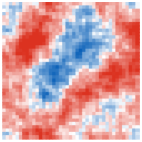
(a)

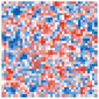
(b)

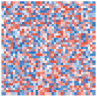
(c)

Figure 4: Three types of random directions of the image space

4.6.2 Results

The robust cost function for the low-frequency directions is

$$R_{\text{low}}^{I}=\frac{1}{c^{2}}\sum_{\begin{subarray}{c}\textrm{training}\\ \textrm{set}\end{subarray}}\left[\sum_{i=1}^{9}\frac{1}{n_{i}^{2}}\left(\frac{\partial N_{i}}{\partial\mathcal{D}_{\text{low}}}-\frac{\partial\mathcal{O}_{i}}{\partial\mathcal{D}_{\text{low}}}\right)^{2}\right].$$ (43)

The error normalization for each output component is based on the range between the 95th and 5th percentiles of the target

$$n_{i}=P_{95}\left[\frac{\partial\mathcal{O}_{i}}{\partial\mathcal{D}_{\text{low}}}\right]-P_{5}\left[\frac{\partial\mathcal{O}_{i}}{\partial\mathcal{D}_{\text{low}}}\right],$$

and $c$ normalizes the average norm of the result

$$c=\text{avg}\left\|\frac{1}{n_{i}}\frac{\partial\mathcal{O}_{i}}{\partial\mathcal{D}_{\text{low}}}\right\|.$$

This allows all gradients to be aligned simultaneously, regardless of their magnitude. Although the optimal adversarials might exploit the one with the largest magnitude, we found that any rebalancing produces worse results. The cost for $\mathcal{D}_{\text{mid}}$ and $\mathcal{D}_{\text{high}}$ are similar. All training parameters are the same as in Subsection 3.5. Random directions are cycled through the set after each epoch. The cost function is

$$E=E_{0}+E_{1}+R_{\text{low}}^{I}+R_{\text{mid}}^{I}.$$

Including the first-order term $E_{1}$ was found to be beneficial, but it adds 6 extra derivatives and it might be more computationally efficient to increase the number of epochs or network capacities instead. The results for the test set are shown in the first 4 columns of the Table III. The values for the training set and the remaining vulnerabilities are almost identical, so they were omitted.

TABLE III: Test error and average maximum vulnerability for networks trained with the first order robust algorithm

weights$\times$106	0.6	1.5	4	12	20*
$e$,%	9.95	5.51	3.12	2.24	1.54
$\bar{v}_{\text{max}}$,%	21.1	17.3	13.3	11.6	7.50

The task is much more demanding, since the networks are now forced to have a certain output in a 1681-dimensional volume, as opposed to a 6-dimensional manifold for the non-robust formulation. Accuracy has taken a significant hit, but it can be improved simultaneously with robustness by increasing the number of weights, adding more layers (while keeping the number of weights constant), adding new directions, decreasing the batch size, or adding more epochs. To demonstrate a combined effect, we train another network with $L=2048$ and two additional hidden layers of 2048 neurons each, using 84 batches with 10% more epochs and a high-frequency term

$$E=E_{0}+E_{1}+R_{\text{low}}^{I}+R_{\text{mid}}^{I}+R_{\text{high}}^{I}.$$

The result is shown in the last column of Table III. The network has 20 million weights, and the asterisk indicates that the training parameters have been changed.

Although robustness and accuracy increase simultaneously as the number of neurons increases, the trade-off between them still exists for a single network, and tuning it could prove useful. By training each network for 1 additional epoch with non-robust cost

$$E=E_{0}+E_{1}$$

we can increase the accuracy 3-4 times in exchange for a slight hit in robustness. The results are shown in Table IV. An example of the gradient of a network with 20 million weights is shown in Fig. 5b

TABLE IV: Error and average vulnerabilities for networks trained with the first-order robust algorithm, trade-off adjusted

weights$\times$106		0.6	1.5	4	12	20*
$e$,%	training	3.66	1.30	0.73	0.54	0.37
	test	3.69	1.33	0.77	0.59	0.46
$\bar{v}_{\text{max}}$,%	training	23.4	18.6	13.9	12.0	7.68
	test	23.5	18.7	14.0	12.1	7.92
$\bar{v}_{\text{sen.}}$,%	training	23.4	18.6	13.9	12.0	7.68
	test	23.4	18.7	14.0	12.1	7.90
$\bar{v}_{\text{inv.}}$,%	training	18.2	15.3	12.3	10.9	7.32
	test	18.2	15.4	12.4	11.0	7.53

(a)

(b)

(c)

Figure 5: Gradients with respect to the first output for the oracle (a), network trained with first-order robust algorithm (b), and network trained with Gaussian augmentation (c)

4.6.3 Gaussian Augmentation

To have a baseline for robust training, we implement a simple data augmentation [46, 47]. For each epoch, Gaussian noise $\mathcal{N_{\sigma}}$ with variance $\sigma^{2}$ and zero mean is added to clean images, so that the problem becomes

$$N\left(\mathcal{I}\left(C\right)+\mathcal{N}_{\sigma}\right)=C.$$ (44)

We start with training all networks with a moderate value of $\sigma=0.055$. The results for clean inputs are in Table V.

TABLE V: Error and average vulnerabilities on clean images for networks trained with Gaussian augmentation, $\sigma=0.055$

weights$\times$106		0.6	1.5	4	12	20*
$e$,%	training	1.87	1.61	1.65	2.31	3.42
	test	2.17	1.93	2.47	3.98	4.91
$\bar{v}_{\text{max}}$,%	training	24.6	21.0	18.0	19.1	24.3
	test	24.7	21.1	18.3	19.6	25.1
$\bar{v}_{\text{sen.}}$,%	training	24.3	20.3	16.5	12.6	8.20
	test	24.3	20.4	17.0	15.6	15.7
$\bar{v}_{\text{inv.}}$,%	training	18.6	16.9	15.2	16.0	18.0
	test	18.7	17.0	15.3	15.6	16.8

The network with 4 million weights has the lowest vulnerability, and larger models overfit in several ways. First, the pockets of invariance are formed around each training pattern, as shown by the overfitting of $\bar{v}_{\text{sen.}}$. This is understandable because the condition (44) forces the network to be locally constant but globally changing, and networks with lower capacity are unable to fit such a target. Second, the networks overfit to the particular amount of Gaussian noise [48]: although the training error on noisy inputs (not shown) decreases slowly with network size, the error on clean test samples (as well as for other $\sigma$) becomes higher.

To see how the noise amplitude affects the results, we pick the best performing architecture with 4 million weights and train it with $\sigma\in\left[0.005,0.17\right]$. The results are shown in Fig. 6 and Fig. 7.

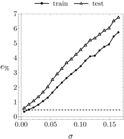
Figure 6: Error on clean images for networks trained with Gaussian augmentation with different $\sigma$. The dashed lines represent the test error for the network trained with the proposed robust algorithm

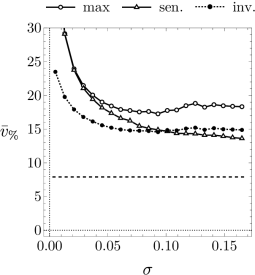
Figure 7: Average vulnerabilities on clean images for networks trained with Gaussian augmentation with different $\sigma$. The dashed lines represent the average maximum vunerability for the network trained with the proposed robust algorithm

Training and test errors grow steadily. The vulnerability to attacks exploiting sensitivity decreases monotonically. However, starting at $\sigma=0.1$, invariance attacks become dominant and the maximum vulnerability starts to increase. This is the reported trade-off between different types of adversarial vulnerabilities [21]. The lowest $v_{\text{max}}=17\%$ is obtained for $\sigma=0.095$, and this network is used for further comparisons. A gradient of the network, shown in Fig. 5c, is “perceptually aligned” [49, 50]. Adding it to the original image resembles a cube motion, but its quality is much lower than that achieved by the proposed robust training. It is clear that the results obtained with Gaussian augmentation hang on the balance between a contradictory cost function and the limited capabilities of the network.

Very similar results can be obtained by minimizing

$$E=E_{0}+c^{2}\sum_{\begin{subarray}{c}\textrm{training}\\ \textrm{set}\end{subarray}}\left\|\partial N/\partial\mathcal{D}\right\|^{2},$$

which is a variant of Jacobian regularization [51, 52, 53, 54]. The main difference with the expression (43) is that the derivative $\partial\mathcal{O}/\partial\mathcal{D}$ is discarded. Even if it is small, as in the case of $\mathcal{D}=\mathcal{D}_{\text{high}}$, neglecting it leads to the same negative effects observed for Gaussian augmentation. As $c^{2}$ is increased from 0, the values of $v_{\text{sen.}}$, $v_{\text{inv.}}$ and $v_{\text{max}}$ decrease, until $v_{\text{max}}$ reaches a minimum of $18\%$, after which, the invariance attacks become dominant, and the maximum vulnerability begins to increase. The best $v_{\text{max}}$ for Gaussian augmentation was $17\%$, therefore, we did not include detailed results. The visual quality of the network gradients is the same as for Gaussian augmentation.

5 Second order

The first-order robust training described in the previous section allows to align the gradients of the network with the oracle only for a set of clean images. As we move away from the 6-dimensional manifold, the alignment weakens and the robustness decreases. The simplest way to extend this alignment further into 1681-dimensional space is to align Hessians for clean images, which can be done by training all second derivatives. In addition, the previous paper [5] reported that the first and second derivatives contributed the most to the relative increase in accuracy, so we expect that for a non-robust problem there will be another sizable accuracy boost. But first, it is necessary to compute the second derivatives of the images with respect to the local coordinates.

5.1 Image Derivatives

The goal is to compute the second derivatives of the cube image with respect to the parameters of the operator (13). Subsection 4.1.1 showed how the first derivatives can be expressed in a closed form and thus computed with machine accuracy. This allows the second derivatives to be computed as a finite difference between the first, evaluated for two close cubes $\hat{T}\left(\pm\varepsilon\delta_{ik}\right)C$

$$\frac{\partial^{2}\mathcal{I}}{\partial\nu_{i}\partial\nu_{j}}\simeq\frac{1}{2\varepsilon}\left(\frac{\partial\mathcal{I}\left(\hat{T}\left(\varepsilon\delta_{ik}\right)C\right)}{\partial\nu_{j}}-\frac{\partial\mathcal{I}\left(\hat{T}\left(-\varepsilon\delta_{ik}\right)C\right)}{\partial\nu_{j}}\right)$$ (45)

With $\varepsilon=5\cdot 10^{-6}$, this produces pixel derivatives with $10^{-6}$ relative precision. Note that the operators $\hat{T}\left(\pm\varepsilon\delta_{ik}\right)$ will form a composition with the operator from the first-order definition (14). For the expression (45) to be consistent with the second derivatives of the original operator (13), the order of the transformations must be preserved. This is true if we consider only $i\leq j$ in the formula (45). This does not mean that the mixed derivatives are not equal, only that if $i>j$ this particular expression corresponds to a derivative of $\hat{T}$ with a different order of operations. In total there are 21 second derivatives, examples are shown in Fig. 8.

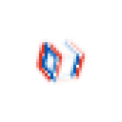
(a)

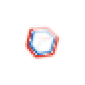
(b)

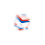
(c)

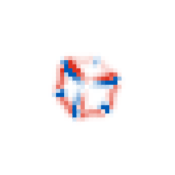
(d)

Figure 8: Second-order image derivatives generated by pairs of infinitesimal operations: Translate $x$ - Translate $x$ (a), Translate $z$ - Translate $z$ (b), Rotate $x$ - Translate $y$ (c) and Rotate $z$ - Rotate $z$ (d)

Denoting the image Hessian

$$\mathcal{H}_{ij}=\frac{\partial^{2}\mathcal{I}}{\partial\nu_{i}\partial\nu_{j}}$$

and combining this with the results of the previous section, we obtain the second order expansions of input and output with respect to the local coordinates $\nu_{i}$

$$\mathcal{I}\left(\hat{T}\left(\nu_{i}\right)C\right)=\mathcal{I}\left(C\right)+\frac{\partial\mathcal{I}}{\partial\nu_{i}}\nu_{i}+\frac{1}{2}\mathcal{H}_{ij}\nu_{i}\nu_{j}+o\left(\nu^{2}\right),$$ (46)

$$\hat{T}\left(\nu_{i}\right)C=C+\frac{\partial C}{\partial\nu_{i}}\nu_{i}+\frac{1}{2}\frac{\partial^{2}C}{\partial\nu_{i}\partial\nu_{j}}\nu_{i}\nu_{j}+o\left(\nu^{2}\right).$$

The second derivatives of $C$ are obtained by differentiating (13) and substituting $\nu_{i}=0$. Most of them are zero, except for the six that specifically pertain to rotations ($i,j\leq 3$)

5.2 Improving Accuracy

The procedure is very similar to that described in Subsection 4.3. The second-order derivatives are now included in the forward pass

$$\mathcal{I},\frac{\partial\mathcal{I}}{\partial\nu_{i}},\frac{\partial^{2}\mathcal{I}}{\partial\nu_{i}\partial\nu_{j}}\overset{\begin{subarray}{c}\textrm{forward}\\ \textrm{pass}\end{subarray}}{\longrightarrow}N,\frac{\partial N}{\partial\nu_{i}},\frac{\partial^{2}N}{\partial\nu_{i}\partial\nu_{j}}.$$

The second order cost function is

$$E_{2}=\sum_{\begin{subarray}{c}\textrm{training}\\ \textrm{set}\end{subarray}}\left[\sum_{i=1}^{6}\sum_{j=i}^{6}\frac{1}{n_{ij}^{2}}\left\|\frac{\partial^{2}N}{\partial\nu_{i}\partial\nu_{j}}-\frac{\partial^{2}\mathcal{O}}{\partial\nu_{i}\partial\nu_{j}}\right\|^{2}\right].$$

The choice of normalization factors $n_{ij}$ is bit more nuanced. For 6 rotational derivatives, the target is non-zero, so we can use

$$n_{ij}=\text{avg}\left\|\frac{\partial^{2}\mathcal{O}}{\partial\nu_{i}\partial\nu_{j}}\right\|,j,i\leq 3.$$

These $n_{ij}$ are close to 1. The average magnitude of the corresponding input derivatives is

$$\underset{j,i\leq 3}{\textrm{avg}}\left\|\frac{\partial\mathcal{I}}{\partial\nu_{i}\partial\nu_{j}}\right\|\simeq 40.$$

Since the outputs are scalable with respect to the inputs, the accuracy scale for the rest of the derivatives can be defined as

$$n_{ij}=40/\textrm{avg}\left\|\frac{\partial\mathcal{I}}{\partial\nu_{i}\partial\nu_{j}}\right\|,i>3.$$

The cost function is

$$E=E_{0}+E_{1}+E_{2}.$$

The initial training lasts for 1950 epochs, then the learning rate is reduced to $l=10^{-4}$ for 25 epochs. Following the approach of gradual exclusion of higher derivatives described in [5], the second derivatives are then dropped and 25 epochs are run with the learning rate $l=10^{-5}$. The results are shown in Table VI. The accuracy of the original problem is increased by a factor of 25 compared to standard training and by a factor of 4 compared to first-order training.

TABLE VI: Error in the initial problem (1) for networks trained with second derivatives

weights$\times$106		0.6	1.5	4	12
$e$,%	training	0.111	0.044	0.017	0.013
	test	0.112	0.046	0.021	0.018

5.3 Oracle Expansion

Similar to first-order robust training, Hessian alignment can be achieved by minimizing the deviation between any second derivatives of the network and the oracle. The second derivatives of the network are computed via forward pass. The second derivative of the oracle is

$$\begin{split}\frac{\partial^{2}\mathcal{O}}{\partial\mathcal{D}^{2}}=\lim_{\varepsilon\rightarrow 0}\frac{1}{\varepsilon^{2}}\Bigl{(}\mathcal{O}\left(\mathcal{I}\left(C\right)+\varepsilon\mathcal{D}\right)+\mathcal{O}&\left(\mathcal{I}\left(C\right)-\varepsilon\mathcal{D}\right)-\\ &-2\mathcal{O}\left(\mathcal{I}\left(C\right)\right)\Bigr{)}.\end{split}$$ (47)

As before, the output of the oracle is written as the transformation of the initial cube

$$\mathcal{O}\left(\mathcal{I}\left(C\right)+\varepsilon\mathcal{D}\right)=\hat{T}\left(\nu_{i}\left(\varepsilon\right)\right)C,$$

for which we now write the second order expansion

$$\nu_{i}\left(\varepsilon\right)=\varepsilon\frac{d\nu_{i}}{d\varepsilon}+\frac{\varepsilon^{2}}{2}\frac{d^{2}\nu_{i}}{d\varepsilon^{2}}+o\left(\varepsilon^{2}\right).$$ (48)

The first term has already been calculated. To get the next term $d^{2}\nu_{i}/d\varepsilon^{2}$, we have to solve a minimization problem

$$\min_{d^{2}\nu_{i}/d\varepsilon^{2}}\left\|\mathcal{I}\left(\hat{T}\left(\varepsilon\frac{d\nu_{i}}{d\varepsilon}+\frac{\varepsilon^{2}}{2}\frac{d^{2}\nu_{i}}{d\varepsilon^{2}}\right)C\right)-\mathcal{I}\left(C\right)-\varepsilon\mathcal{D}\right\|^{2}.$$ (49)

Substituting (48) into the second-order expansion of images (46) gives

$$\begin{split}&\mathcal{I}\left(\hat{T}\left(\varepsilon\frac{d\nu_{i}}{d\varepsilon}+\frac{\varepsilon^{2}}{2}\frac{d^{2}\nu_{i}}{d\varepsilon^{2}}\right)C\right)=\mathcal{I}\left(C\right)+\varepsilon\frac{\partial\mathcal{I}}{\partial\nu_{i}}\frac{d\nu_{i}}{d\varepsilon}+\\ &+\frac{\varepsilon^{2}}{2}\left(\frac{\partial\mathcal{I}}{\partial\nu_{i}}\frac{d^{2}\nu_{i}}{d\varepsilon^{2}}+\mathcal{H}_{ij}\frac{d\nu_{i}}{d\varepsilon}\frac{d\nu_{j}}{d\varepsilon}\right)+\frac{\varepsilon^{3}}{2}\mathcal{H}_{ij}\frac{d\nu_{i}}{d\varepsilon}\frac{d^{2}\nu_{j}}{d\varepsilon^{2}}.\end{split}$$ (50)

The last summand may seem out of order, but the the third-order expansion terms proportional to $\varepsilon^{3}$ do not depend on $d^{2}\nu_{i}/d\varepsilon^{2}$, which means that for our purposes this relationship is actually $o\left(\varepsilon^{3}\right)$ accurate. After substituting it into (49) and expanding the squared norm, terms proportional to $\varepsilon^{3}$ cancel out when we consider the first-order relation (23). So we only need to consider terms proportional to $\varepsilon^{4}$:

$$\min_{d^{2}\nu_{i}/d\varepsilon^{2}}\left[\left(\frac{\partial\mathcal{I}}{\partial\nu_{i}}\frac{d\nu_{i}}{d\varepsilon}-\mathcal{D}\right)\cdot\mathcal{H}_{ij}\frac{d\nu_{i}}{d\varepsilon}\frac{d^{2}\nu_{j}}{d\varepsilon^{2}}\right.+$$

$$\left.+\frac{1}{4}\left\|\frac{\partial\mathcal{I}}{\partial\nu_{i}}\frac{d^{2}\nu_{i}}{d\varepsilon^{2}}+\mathcal{H}_{ij}\frac{d\nu_{i}}{d\varepsilon}\frac{d\nu_{j}}{d\varepsilon}\right\|^{2}\right].$$

by expanding the squared norm and taking derivatives with respect to $d^{2}\nu_{i}/d\varepsilon^{2}$ we get a system of 6 equations

$$\begin{split}\Gamma_{ij}\frac{d^{2}\nu_{j}}{d\varepsilon^{2}}&=2\left(\mathcal{D}\cdot\mathcal{H}_{ik}\right)\frac{d\nu_{k}}{d\varepsilon}-2\left(\mathcal{H}_{ki}\cdot\frac{\partial\mathcal{I}}{\partial\nu_{p}}\right)\frac{d\nu_{p}}{d\varepsilon}\frac{d\nu_{k}}{d\varepsilon}-\\ &-\left(\mathcal{H}_{kp}\cdot\frac{\partial\mathcal{I}}{\partial\nu_{i}}\right)\frac{d\nu_{p}}{d\varepsilon}\frac{d\nu_{k}}{d\varepsilon}.\end{split}$$ (51)

Similar to (23), the solution is obtained using $\Gamma^{-1}$. The output of the oracle is

$$\mathcal{O}\left(\mathcal{I}\left(C\right)+\varepsilon\mathcal{D}\right) =C+\varepsilon\frac{\partial C}{\partial\nu_{i}}\frac{d\nu_{i}}{d\varepsilon}+$$

$$+\frac{\varepsilon^{2}}{2}\left(\frac{\partial C}{\partial\nu_{i}}\frac{\partial^{2}\nu_{i}}{d\varepsilon^{2}}+\frac{\partial^{2}C}{\partial\nu_{i}\partial\nu_{j}}\frac{d\nu_{j}}{d\varepsilon}\frac{d\nu_{i}}{d\varepsilon}\right)+o\left(\varepsilon^{2}\right),$$

by substituting it into (47) we get

$$\frac{\partial^{2}\mathcal{O}}{\partial\mathcal{D}^{2}}=\frac{\partial C}{\partial\nu_{i}}\frac{\partial^{2}\nu_{i}}{d\varepsilon^{2}}+\frac{\partial^{2}C}{\partial\nu_{i}\partial\nu_{j}}\frac{d\nu_{i}}{d\varepsilon}\frac{d\nu_{j}}{d\varepsilon}.$$

Here $d\nu_{j}/d\varepsilon$ is the solution of (23) and $\partial^{2}\nu_{i}/d\varepsilon^{2}$ is the solution of (51).

5.4 Universal Robust Training

The second-order robust cost and its normalization are similar to the first-order formulas

$$R_{\text{low}}^{I\!I}=\frac{1}{c^{2}}\sum_{\begin{subarray}{c}\textrm{training}\\ \textrm{set}\end{subarray}}\left[\sum_{i=1}^{9}\frac{1}{n_{i}^{2}}\left(\frac{\partial^{2}N_{i}}{\partial\mathcal{D}_{\text{low}}^{2}}-\frac{\partial^{2}\mathcal{O}_{i}}{\partial\mathcal{D}_{\text{low}}^{2}}\right)^{2}\right],$$

$$n_{i}=P_{95}\left[\frac{\partial^{2}\mathcal{O}_{i}}{\partial\mathcal{D}_{\text{low}}^{2}}\right]-P_{5}\left[\frac{\partial^{2}\mathcal{O}_{i}}{\partial\mathcal{D}_{\text{low}}^{2}}\right],$$

$$c=\text{avg}\left\|\frac{1}{n_{i}}\frac{\partial^{2}\mathcal{O}_{i}}{\partial\mathcal{D}_{\text{low}}^{2}}\right\|,$$

with equivalent expressions for $\mathcal{D}_{\text{mid}}$ and $\mathcal{D}_{\text{high}}$. The first 4 networks are trained with

$$E=E_{0}+E_{1}+R_{\text{low}}^{I}+R_{\text{mid}}^{I}+R_{\text{low}}^{I\!I}+R_{\text{mid}}^{I\!I}.$$

The addition of $E_{2}$ did not improve the results. All training parameters are the same as in Subsection 4.6. For the network with $20\cdot 10^{6}$ weights, two additional terms are included $R_{\text{high}}^{I}+R_{\text{high}}^{I\!I}$. The results for the clean images from the test set are shown in Table VII. The values for the training set and the remaining vulnerabilities are almost identical, so they were omitted.

TABLE VII: Test error and average maximum vulnerability for networks trained with the second-order robust algorithm

weights$\times$106	0.6	1.5	4	12	20*
$e$,%	22.9	14.9	8.42	6.21	4.71
$\bar{v}_{\text{max}}$,%	20.4	17.0	13.0	11.2	7.20

As before, by adding an extra epoch with the cost function $E=E_{0}+E_{1}$, we can increase the precision a few times in exchange for a small hit in robustness. The results are shown in Table VIII. Apart from a slight hit in accuracy and a larger gap between networks, the results are very similar to the first-order training.

TABLE VIII: Error and average vulnerabilities for networks trained with the second-order robust algorithm, trade-off adjusted

weights$\times$106		0.6	1.5	4	12	20*
$e$,%	training	12.7	5.59	1.90	1.20	0.69
	test	12.7	5.62	1.92	1.23	0.73
$\bar{v}_{\text{max}}$,%	training	22.4	18.8	14.1	12.0	7.50
	test	22.4	18.9	14.2	12.1	7.58
$\bar{v}_{\text{sen.}}$,%	training	20.7	18.4	14.1	12.0	7.48
	test	20.7	18.5	14.1	12.1	7.55
$\bar{v}_{\text{inv.}}$,%	training	19.6	16.3	12.7	11.0	7.22
	test	19.6	16.4	12.7	11.1	7.29

However, the purpose of the second-order training was to extend the robustness further into the image space. To see if it worked, we will investigate the accuracy and maximum vulnerability under Gaussian noise of various magnitudes. Adding the noise can change the value of the oracle, so the minimization problem (9) has to be solved. Fortunately, for $\sigma\leq 0.25$ the Gaussian noise produces relatively small changes that can be accurately captured using the Taylor expansion (10). Substituting $\mathcal{D}=\mathcal{N}_{\sigma}$ and $\varepsilon=1$, we get

$$\mathcal{O}\left(\mathcal{I}+\mathcal{N}_{\sigma}\right)\simeq\mathcal{O}\left(\mathcal{I}\right)+\frac{\partial\mathcal{O}}{\partial\mathcal{N}_{\sigma}}+\frac{1}{2}\frac{\partial^{2}\mathcal{O}}{\partial\mathcal{N}_{\sigma}^{2}}.$$ (52)

For $\sigma\leq 0.25$, the first order term dominates the adjustment, and the second derivative contributes up to 1/20 of the correction. This formula provides the vertices of the new cube for which the image derivatives are generated and the maximum vulnerability is determined by solving (34). We compare the results of the first ($I$) and second ($I\!I$) order robust training of the network with $20\cdot 10^{6}$ weights against the best result of Gaussian augmentation ($\mathcal{N}_{.095}$). Fig. 9 shows the comparison of the errors, the results without adjustment (52) are shown in color. We observe that for all networks the corrected accuracy is higher, and for $I$ and $I\!I$ the amount of correction is substantial even for small $\sigma$. For large $\sigma$, the accuracy of $I$ becomes lower than $\mathcal{N}_{.095}$, but the results of $I\!I$ are unmatched.

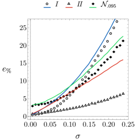
Figure 9: Error under Gaussian noise for networks trained with the first- ($I$), second-order ($I\!I$) robust algorithm and the best result of Gaussian augmentation ($\mathcal{N}_{.095}$)

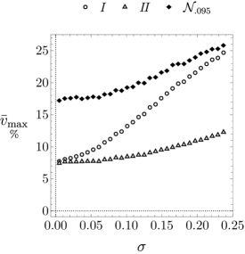
Figure 10: Average maximum vulnerability under Gaussian noise for networks trained with the first- ($I$), second-order ($I\!I$) robust algorithm and the best result of Gaussian augmentation ($\mathcal{N}_{.095}$)

Fig. 10 shows the average maximum vulnerabilities. The results without correction (52) are not more than 1% different, so they are not shown. Network $I$ gradually loses its robustness, but as expected, the second-order results are much more stable. The effect of adding an extra epoch with $E=E_{0}+E_{1}$ is uniform across $\sigma$ for both plots.

It is worth noting that for $\sigma=0.25$ the distance between the original and the noisy image is $\sim$10, which is roughly the diameter of the manifold. Thus, training the derivatives only on the manifold allows to obtain a reasonable error in a significant volume of the full image space.

6 Related Work

6.1 Robust Training

Since standard adversarial training against sensitivity-based attacks usually comes at the cost of accuracy [23, 22, 29], several works have been devoted to improving this trade-off [55, 56, 57, 58, 59]. Works [28, 27] presented the evidence that this trade-off can be avoided entirely. The discovery of invariance-based attacks introduced another robustness metric, which turned out to be incompatible with the previous one [21, 60]. The trade-off between two types of robustness and accuracy was approached with Pareto optimization [30] as well as other balancing methods [31, 33]. Work [32] suggested weakening the invariance radius for each input separately. In this paper, we have shown how both types of robustness can be achieved simultaneously with high accuracy, with network capacity seemingly the only limiting factor.

6.2 Training Derivatives

There are two different approaches to training derivatives. The first, which is the most common, uses them as a regularization for the initial problem [61]. It can be written as $D\left(N\right)=0$ for any order or type of derivative. This was introduced in [51, 62] for classifiers, in [63, 64] for autoencoders, in [65, 66, 67] for generative adversarial networks. It can also be implemented for adversarial training [68, 69, 67, 66, 52, 53, 54]. As we saw, such conditions can easily conflict with non-zero oracle gradients and cause a trade-off between different types of vulnerability. It does not allow to increase the accuracy of the original problem.

The second, less common approach is to enforce the condition $D\left(N\right)=D\left(\mathcal{O}\right)$ with non-zero right side as an addition to the objective $N=\mathcal{O}$. This idea has been implemented in [70, 71, 72, 73, 74, 75] with moderate success. The author’s paper [5] showed how this method can significantly increase the accuracy of the initial objective. This paper showcases similar success in addressing a simple image analysis problem.

Another relevant area dealing exclusively with training derivatives is the solution of differential equations using neural networks [76, 77, 78, 79, 80, 81]. In this case, $D$ is the differential operator of the equation, accompanied by initial and/or boundary conditions. The input of the network is a vector of independent variables, and the output is the value of the solution. The weights are trained so that the residual $D\left(N\right)$ approaches zero and boundary conditions are satisfied. The flexibility of the training process allows solving under-, overdetermined [82] and inverse problems [83, 84].

6.3 Tangent Plane

The results of Section 4 are based on the first-order analysis. It can be similarly implemented by a geometric approach, where the data manifold is locally represented by a tangent plane. We will mention the papers where tangent planes have been constructed and used for network training. All of them use derivatives as regularization, as described in Subsection 6.2.

In [62] a classifier for handwritten digits (MNIST) is considered. The tangent plane for each image is constructed as a linear space of infinitesimal rotations, translations, and deformations. A cost function ensures the invariance of the classifier under tangential perturbations.

In [85], classifiers for MNIST and color images of 10 different classes (CIFAR-10) are trained to remain constant under perturbations restricted to the tangent plane. The plane is constructed using a contractive autoencoder [63].

In [86] the classification task is solved for CIFAR-10 and color street numbers (SVHN). An additional cost function enforces the invariance with respect to tangential perturbations. The plane is constructed via the generator part of the Generative Adversarial Network (GAN).

In work [87] classifiers for SVHN, CIFAR-10 and grayscale fashion items in 10 categories (FashionMNIST) are considered. The tangent plane is constructed by variational autoencoder and localized GAN [66]. Tangential perturbations are regularized based on virtual adversarial training. Additional regularization with respect to orthogonal perturbations is used to enforce robustness.

6.4 Tracking Problems

Although the goal of the object tracking is to determine a bounding box, a number of works achieve this by reconstructing the object being tracked. This can be done by minimizing some norm with respect to the parameters of low-dimensional representation, which is similar to the minimization we performed to construct the oracle. Low-dimensional representations can be obtained by neural networks [88, 89], principal component analysis [90, 91, 92] or dictionary learning [93]. The robustness of methods that do not use deep neural networks is naturally higher, while in this paper we focused on training a robust deep network.

7 Conclusion

The purpose of this study was to show that for the image analysis problem, network accuracy can be significantly improved on both noiseless and noisy inputs by training derivatives. In addition, we showed how the reported trade-off between two types of robustness can be eliminated, as both increase by a factor of 2.3 compared to Gaussian augmentation and Jacobian regularization.

It is worth noting that discriminative classification is incompatible with the proposed approach. Even if a class manifold is fully known, any movement along the manifold will not change the output of the classifier, and small orthogonal movements will not change the nearest class. Larger orthogonal movements can change the output, but the increment would depend on the relative position and shape of the other class manifolds. This means that the local behavior of the discriminative classifier is determined by the entire set of classes, while our approach is purely local. In contrast, in score-based generative classification [94, 95] each class has a generator, that provides the closest member for a given input. The answer is then determined based on the best match. Since each generator is described by a single manifold, the non-locality is avoided. So far, generative classifiers are not more robust [95, 96] than discriminative models.

In general, this paper has outlined a promising direction for further research. Tracking degrees of freedom is useful when the object is more complex, such as a walking human. A reasonable model for this has 30 degrees of freedom, and since the number of first derivatives increases linearly, this seems like an achievable goal. It would require a more powerful rendering algorithm compatible with numerical differentiation. Different lighting, textures and backgrounds would create multiple “parallel” manifolds for which the presented training is applicable. The transitions between the manifolds can be considered as perturbations and can be handled by robust training. This may produce a neural network that is provably accurate over a substantial volume of the full image space. Finally, studying a relatively small number of objects from different angles is more consistent with human development than learning on thousands of individual images, and understanding the pose of the object is a critical part of the visual recognition process.

Vsevolod I. Avrutskiy Received a Ph.D. in Machine Learning for Mathematical Physics from Moscow Institute of Physics and Technology (MIPT) in 2021. Worked at MIPT as a teacher in the Department of Theoretical Physics, Department of Computer Modelling, and as a researcher in the Laboratory of Theoretical Attosecond Physics. Current research interests include training neural network derivatives, shape optimization, and solving partial differential equations with neural networks.

References

- [1] K. Hornik, “Approximation capabilities of multilayer feedforward networks,” Neural networks, vol. 4, no. 2, pp. 251–257, 1991, publisher: Elsevier.
- [2] V. Kurková, “Kolmogorov’s theorem and multilayer neural networks,” Neural networks, vol. 5, no. 3, pp. 501–506, 1992, publisher: Elsevier.
- [3] A. R. Barron, “Approximation and estimation bounds for artificial neural networks,” Machine learning, vol. 14, pp. 115–133, 1994, publisher: Springer.
- [4] Y. LeCun, Y. Bengio, and G. Hinton, “Deep learning,” nature, vol. 521, no. 7553, pp. 436–444, 2015, publisher: Nature Publishing Group UK London.
- [5] V. I. Avrutskiy, “Enhancing function approximation abilities of neural networks by training derivatives,” IEEE transactions on neural networks and learning systems, vol. 32, no. 2, pp. 916–924, 2020, publisher: IEEE.
- [6] ——, “Neural networks catching up with finite differences in solving partial differential equations in higher dimensions,” Neural Computing and Applications, vol. 32, no. 17, pp. 13 425–13 440, 2020, publisher: Springer.
- [7] H. Montes-Campos, J. Carrete, S. Bichelmaier, L. M. Varela, and G. K. Madsen, “A differentiable neural-network force field for ionic liquids,” Journal of chemical information and modeling, vol. 62, no. 1, pp. 88–101, 2021, publisher: ACS Publications.
- [8] J. Carrete, H. Montes-Campos, R. Wanzenböck, E. Heid, and G. K. Madsen, “Deep ensembles vs committees for uncertainty estimation in neural-network force fields: Comparison and application to active learning,” The Journal of Chemical Physics, vol. 158, no. 20, 2023, publisher: AIP Publishing.
- [9] Y. Kim, H. Lee, and J. Ryu, “Learning an accurate state transition dynamics model by fitting both a function and its derivative,” IEEE Access, vol. 10, pp. 44 248–44 258, 2022, publisher: IEEE.
- [10] S.-M. Wang and R. Kikuuwe, “Neural Encoding of Mass Matrices of Articulated Rigid-body Systems in Cholesky-Decomposed Form,” in 2022 IEEE International Conference on Industrial Technology (ICIT). IEEE, 2022, pp. 1–8.
- [11] V. Istomin, E. Kustova, S. Lagutin, and I. Shalamov, “Evaluation of state-specific transport properties using machine learning methods,” Cybernetics and Physics, vol. 12, no. 1, pp. 34–41, 2023.
- [12] W. M. Kwok, G. Streftaris, and S. C. Dass, “Laplace based Bayesian inference for ordinary differential equation models using regularized artificial neural networks,” Statistics and Computing, vol. 33, no. 6, p. 124, 2023, publisher: Springer.
- [13] L. Cayton, Algorithms for manifold learning. eScholarship, University of California, 2008.
- [14] C. Fefferman, S. Mitter, and H. Narayanan, “Testing the manifold hypothesis,” Journal of the American Mathematical Society, vol. 29, no. 4, pp. 983–1049, 2016.
- [15] C. Szegedy, W. Zaremba, I. Sutskever, J. Bruna, D. Erhan, I. Goodfellow, and R. Fergus, “Intriguing properties of neural networks,” arXiv preprint arXiv:1312.6199, 2013.
- [16] C. Lyu, K. Huang, and H.-N. Liang, “A unified gradient regularization family for adversarial examples,” in 2015 IEEE international conference on data mining. IEEE, 2015, pp. 301–309.
- [17] I. J. Goodfellow, J. Shlens, and C. Szegedy, “Explaining and harnessing adversarial examples,” arXiv preprint arXiv:1412.6572, 2014.
- [18] T. Bai, J. Luo, J. Zhao, B. Wen, and Q. Wang, “Recent advances in adversarial training for adversarial robustness,” arXiv preprint arXiv:2102.01356, 2021.
- [19] J.-H. Jacobsen, J. Behrmann, R. Zemel, and M. Bethge, “Excessive invariance causes adversarial vulnerability,” arXiv preprint arXiv:1811.00401, 2018.
- [20] J.-H. Jacobsen, J. Behrmannn, N. Carlini, F. Tramer, and N. Papernot, “Exploiting excessive invariance caused by norm-bounded adversarial robustness,” arXiv preprint arXiv:1903.10484, 2019.
- [21] F. Tramèr, J. Behrmann, N. Carlini, N. Papernot, and J.-H. Jacobsen, “Fundamental tradeoffs between invariance and sensitivity to adversarial perturbations,” in International Conference on Machine Learning. PMLR, 2020, pp. 9561–9571.
- [22] D. Su, H. Zhang, H. Chen, J. Yi, P.-Y. Chen, and Y. Gao, “Is Robustness the Cost of Accuracy?–A Comprehensive Study on the Robustness of 18 Deep Image Classification Models,” in Proceedings of the European conference on computer vision (ECCV), 2018, pp. 631–648.
- [23] D. Tsipras, S. Santurkar, L. Engstrom, A. Turner, and A. Madry, “Robustness may be at odds with accuracy,” arXiv preprint arXiv:1805.12152, 2018.
- [24] H. Zhang, Y. Yu, J. Jiao, E. Xing, L. El Ghaoui, and M. Jordan, “Theoretically principled trade-off between robustness and accuracy,” in International conference on machine learning. PMLR, 2019, pp. 7472–7482.
- [25] S. Kamath, A. Deshpande, S. Kambhampati Venkata, and V. N Balasubramanian, “Can we have it all? On the Trade-off between Spatial and Adversarial Robustness of Neural Networks,” Advances in Neural Information Processing Systems, vol. 34, pp. 27 462–27 474, 2021.
- [26] M. Moayeri, K. Banihashem, and S. Feizi, “Explicit tradeoffs between adversarial and natural distributional robustness,” Advances in Neural Information Processing Systems, vol. 35, pp. 38 761–38 774, 2022.
- [27] D. Stutz, M. Hein, and B. Schiele, “Disentangling adversarial robustness and generalization,” in Proceedings of the IEEE/CVF Conference on Computer Vision and Pattern Recognition, 2019, pp. 6976–6987.
- [28] P. Nakkiran, “Adversarial robustness may be at odds with simplicity,” arXiv preprint arXiv:1901.00532, 2019.
- [29] E. Dobriban, H. Hassani, D. Hong, and A. Robey, “Provable tradeoffs in adversarially robust classification,” IEEE Transactions on Information Theory, 2023, publisher: IEEE.
- [30] L. Z. Sun Ke, Li Mingjie, “Pareto Adversarial Robustness: Balancing Spatial Robustness and Sensitivity-based Robustness,” SCIENCE CHINA Information Sciences, pp. –, 2023.
- [31] H. Chen, Y. Ji, and D. Evans, “Balanced adversarial training: Balancing tradeoffs between fickleness and obstinacy in NLP models,” arXiv preprint arXiv:2210.11498, 2022.
- [32] S. Yang and C. Xu, “One Size Does NOT Fit All: Data-Adaptive Adversarial Training,” in European Conference on Computer Vision. Springer, 2022, pp. 70–85.
- [33] R. Rauter, M. Nocker, F. Merkle, and P. Schöttle, “On the Effect of Adversarial Training Against Invariance-based Adversarial Examples,” in Proceedings of the 2023 8th International Conference on Machine Learning Technologies, Mar. 2023, pp. 54–60, arXiv:2302.08257 [cs].
- [34] M. Riedmiller and H. Braun, “A direct adaptive method for faster backpropagation learning: The RPROP algorithm,” in IEEE international conference on neural networks. IEEE, 1993, pp. 586–591.
- [35] J. Bloomenthal and J. Rokne, “Homogeneous coordinates,” The Visual Computer, vol. 11, no. 1, pp. 15–26, Jan. 1994.
- [36] C. S. Williams and O. A. Becklund, Introduction to the optical transfer function. SPIE Press, 2002, vol. 112.
- [37] A. N. Korobov, “The approximate computation of multiple integrals,” in Dokl. Akad. Nauk SSSR, vol. 124, 1959, pp. 1207–1210.
- [38] I. O. Tolstikhin, N. Houlsby, A. Kolesnikov, L. Beyer, X. Zhai, T. Unterthiner, J. Yung, A. Steiner, D. Keysers, and J. Uszkoreit, “Mlp-mixer: An all-mlp architecture for vision,” Advances in neural information processing systems, vol. 34, pp. 24 261–24 272, 2021.
- [39] X. Glorot and Y. Bengio, “Understanding the difficulty of training deep feedforward neural networks,” in Proceedings of the thirteenth international conference on artificial intelligence and statistics. JMLR Workshop and Conference Proceedings, 2010, pp. 249–256.
- [40] K. He, X. Zhang, S. Ren, and J. Sun, “Delving deep into rectifiers: Surpassing human-level performance on imagenet classification,” in Proceedings of the IEEE international conference on computer vision, 2015, pp. 1026–1034.
- [41] D. P. Kingma and J. Ba, “Adam: A method for stochastic optimization,” arXiv preprint arXiv:1412.6980, 2014.
- [42] Z. Qian, K. Huang, Q.-F. Wang, and X.-Y. Zhang, “A survey of robust adversarial training in pattern recognition: Fundamental, theory, and methodologies,” Pattern Recognition, vol. 131, p. 108889, 2022, publisher: Elsevier.
- [43] A. Madry, A. Makelov, L. Schmidt, D. Tsipras, and A. Vladu, “Towards deep learning models resistant to adversarial attacks,” arXiv preprint arXiv:1706.06083, 2017.
- [44] E. G. Hemingway and O. M. O’Reilly, “Perspectives on Euler angle singularities, gimbal lock, and the orthogonality of applied forces and applied moments,” Multibody System Dynamics, vol. 44, no. 1, pp. 31–56, Sep. 2018.
- [45] V. I. Avrutskiy, “Preventing overfitting by training derivatives,” in Proceedings of the Future Technologies Conference (FTC) 2019: Volume 1. Springer, 2020, pp. 144–163.
- [46] V. Zantedeschi, M.-I. Nicolae, and A. Rawat, “Efficient defenses against adversarial attacks,” in Proceedings of the 10th ACM Workshop on Artificial Intelligence and Security, 2017, pp. 39–49.
- [47] J. Gilmer, N. Ford, N. Carlini, and E. Cubuk, “Adversarial examples are a natural consequence of test error in noise,” in International Conference on Machine Learning. PMLR, 2019, pp. 2280–2289.
- [48] K. Kireev, M. Andriushchenko, and N. Flammarion, “On the effectiveness of adversarial training against common corruptions,” in Uncertainty in Artificial Intelligence. PMLR, 2022, pp. 1012–1021.
- [49] S. Santurkar, A. Ilyas, D. Tsipras, L. Engstrom, B. Tran, and A. Madry, “Image synthesis with a single (robust) classifier,” Advances in Neural Information Processing Systems, vol. 32, 2019.
- [50] S. Kaur, J. Cohen, and Z. C. Lipton, “Are perceptually-aligned gradients a general property of robust classifiers?” arXiv preprint arXiv:1910.08640, 2019.
- [51] H. Drucker and Y. Le Cun, “Improving generalization performance using double backpropagation,” IEEE transactions on neural networks, vol. 3, no. 6, pp. 991–997, 1992.
- [52] D. Jakubovitz and R. Giryes, “Improving dnn robustness to adversarial attacks using jacobian regularization,” in Proceedings of the European conference on computer vision (ECCV), 2018, pp. 514–529.
- [53] J. Hoffman, D. A. Roberts, and S. Yaida, “Robust Learning with Jacobian Regularization,” Aug. 2019, arXiv:1908.02729 [cs, stat].
- [54] A. Chan, Y. Tay, Y. S. Ong, and J. Fu, “Jacobian Adversarially Regularized Networks for Robustness,” Jan. 2020, arXiv:1912.10185 [cs].
- [55] T. Tanay and L. Griffin, “A boundary tilting persepective on the phenomenon of adversarial examples,” arXiv preprint arXiv:1608.07690, 2016.
- [56] R. G. Lopes, D. Yin, B. Poole, J. Gilmer, and E. D. Cubuk, “Improving robustness without sacrificing accuracy with patch gaussian augmentation,” arXiv preprint arXiv:1906.02611, 2019.
- [57] E. Arani, F. Sarfraz, and B. Zonooz, “Adversarial concurrent training: Optimizing robustness and accuracy trade-off of deep neural networks,” arXiv preprint arXiv:2008.07015, 2020.
- [58] T.-K. Hu, T. Chen, H. Wang, and Z. Wang, “Triple wins: Boosting accuracy, robustness and efficiency together by enabling input-adaptive inference,” arXiv preprint arXiv:2002.10025, 2020.
- [59] Y.-Y. Yang, C. Rashtchian, H. Zhang, R. R. Salakhutdinov, and K. Chaudhuri, “A closer look at accuracy vs. robustness,” Advances in neural information processing systems, vol. 33, pp. 8588–8601, 2020.
- [60] V. Singla, S. Ge, B. Ronen, and D. Jacobs, “Shift invariance can reduce adversarial robustness,” Advances in Neural Information Processing Systems, vol. 34, pp. 1858–1871, 2021.
- [61] M. Belkin, P. Niyogi, and V. Sindhwani, “Manifold regularization: A geometric framework for learning from labeled and unlabeled examples.” Journal of machine learning research, vol. 7, no. 11, 2006.
- [62] P. Y. Simard, Y. A. LeCun, J. S. Denker, and B. Victorri, “Transformation Invariance in Pattern Recognition — Tangent Distance and Tangent Propagation,” in Neural Networks: Tricks of the Trade, G. Goos, J. Hartmanis, J. Van Leeuwen, G. B. Orr, and K.-R. Müller, Eds. Berlin, Heidelberg: Springer Berlin Heidelberg, 1998, vol. 1524, pp. 239–274, series Title: Lecture Notes in Computer Science.
- [63] S. Rifai, P. Vincent, X. Muller, X. Glorot, and Y. Bengio, “Contractive auto-encoders: Explicit invariance during feature extraction,” in Proceedings of the 28th international conference on international conference on machine learning, 2011, pp. 833–840.
- [64] S. Rifai, G. Mesnil, P. Vincent, X. Muller, Y. Bengio, Y. Dauphin, and X. Glorot, “Higher order contractive auto-encoder,” in Machine Learning and Knowledge Discovery in Databases: European Conference, ECML PKDD 2011, Athens, Greece, September 5-9, 2011, Proceedings, Part II 22. Springer, 2011, pp. 645–660.
- [65] K. Roth, A. Lucchi, S. Nowozin, and T. Hofmann, “Stabilizing training of generative adversarial networks through regularization,” Advances in neural information processing systems, vol. 30, 2017.
- [66] G.-J. Qi, L. Zhang, H. Hu, M. Edraki, J. Wang, and X.-S. Hua, “Global versus localized generative adversarial nets,” in Proceedings of the IEEE conference on computer vision and pattern recognition, 2018, pp. 1517–1525.
- [67] B. Lecouat, C.-S. Foo, H. Zenati, and V. R. Chandrasekhar, “Semi-supervised learning with gans: Revisiting manifold regularization,” arXiv preprint arXiv:1805.08957, 2018.
- [68] T. Miyato, S.-i. Maeda, M. Koyama, and S. Ishii, “Virtual adversarial training: a regularization method for supervised and semi-supervised learning,” IEEE transactions on pattern analysis and machine intelligence, vol. 41, no. 8, pp. 1979–1993, 2018, publisher: IEEE.
- [69] A. Ross and F. Doshi-Velez, “Improving the adversarial robustness and interpretability of deep neural networks by regularizing their input gradients,” in Proceedings of the AAAI conference on artificial intelligence, vol. 32, 2018, issue: 1.
- [70] P. Cardaliaguet and G. Euvrard, “Approximation of a function and its derivative with a neural network,” Neural networks, vol. 5, no. 2, pp. 207–220, 1992, publisher: Elsevier.
- [71] E. Basson and A. P. Engelbrecht, “Approximation of a function and its derivatives in feedforward neural networks,” in IJCNN’99. International Joint Conference on Neural Networks. Proceedings (Cat. No. 99CH36339), vol. 1. IEEE, 1999, pp. 419–421.
- [72] G. Flake and B. Pearlmutter, “Differentiating Functions of the Jacobian with Respect to the Weights,” Advances in Neural Information Processing Systems, vol. 12, 1999.
- [73] S. He, K. Reif, and R. Unbehauen, “Multilayer neural networks for solving a class of partial differential equations,” Neural networks, vol. 13, no. 3, pp. 385–396, 2000, publisher: Elsevier.
- [74] A. Pukrittayakamee, M. Hagan, L. Raff, S. T. Bukkapatnam, and R. Komanduri, “Practical training framework for fitting a function and its derivatives,” IEEE transactions on neural networks, vol. 22, no. 6, pp. 936–947, 2011, publisher: IEEE.
- [75] W. Yuan, Q. Zhu, X. Liu, Y. Ding, H. Zhang, and C. Zhang, “Sobolev training for implicit neural representations with approximated image derivatives,” in European Conference on Computer Vision. Springer, 2022, pp. 72–88.
- [76] A. J. Meade Jr and A. A. Fernandez, “The numerical solution of linear ordinary differential equations by feedforward neural networks,” Mathematical and Computer Modelling, vol. 19, no. 12, pp. 1–25, 1994, publisher: Elsevier.
- [77] I. E. Lagaris, A. Likas, and D. I. Fotiadis, “Artificial neural network methods in quantum mechanics,” Computer Physics Communications, vol. 104, no. 1-3, pp. 1–14, 1997, publisher: Elsevier.
- [78] ——, “Artificial neural networks for solving ordinary and partial differential equations,” IEEE transactions on neural networks, vol. 9, no. 5, pp. 987–1000, 1998, publisher: IEEE.
- [79] E. M. Budkina, E. B. Kuznetsov, T. V. Lazovskaya, S. S. Leonov, D. A. Tarkhov, and A. N. Vasilyev, “Neural network technique in boundary value problems for ordinary differential equations,” in Advances in Neural Networks–ISNN 2016: 13th International Symposium on Neural Networks, ISNN 2016, St. Petersburg, Russia, July 6-8, 2016, Proceedings 13. Springer, 2016, pp. 277–283.
- [80] D. Tarkhov and A. N. Vasilyev, Semi-empirical neural network modeling and digital twins development. Academic Press, 2019.
- [81] M. Kumar and N. Yadav, “Multilayer perceptrons and radial basis function neural network methods for the solution of differential equations: a survey,” Computers & Mathematics with Applications, vol. 62, no. 10, pp. 3796–3811, 2011, publisher: Elsevier.
- [82] G. E. Karniadakis, I. G. Kevrekidis, L. Lu, P. Perdikaris, S. Wang, and L. Yang, “Physics-informed machine learning,” Nature Reviews Physics, vol. 3, no. 6, pp. 422–440, 2021, publisher: Nature Publishing Group UK London.
- [83] V. I. Gorbachenko, T. V. Lazovskaya, D. A. Tarkhov, A. N. Vasilyev, and M. V. Zhukov, “Neural network technique in some inverse problems of mathematical physics,” in Advances in Neural Networks–ISNN 2016: 13th International Symposium on Neural Networks, ISNN 2016, St. Petersburg, Russia, July 6-8, 2016, Proceedings 13. Springer, 2016, pp. 310–316.
- [84] V. I. Gorbachenko and D. A. Stenkin, “Solving of Inverse Coefficient Problems on Networks of Radial Basis Functions,” in Advances in Neural Computation, Machine Learning, and Cognitive Research V, B. Kryzhanovsky, W. Dunin-Barkowski, V. Redko, Y. Tiumentsev, and V. V. Klimov, Eds. Cham: Springer International Publishing, 2022, vol. 1008, pp. 230–237, series Title: Studies in Computational Intelligence.
- [85] S. Rifai, Y. N. Dauphin, P. Vincent, Y. Bengio, and X. Muller, “The manifold tangent classifier,” Advances in neural information processing systems, vol. 24, 2011.
- [86] A. Kumar, P. Sattigeri, and T. Fletcher, “Semi-supervised learning with gans: Manifold invariance with improved inference,” Advances in neural information processing systems, vol. 30, 2017.
- [87] B. Yu, J. Wu, J. Ma, and Z. Zhu, “Tangent-normal adversarial regularization for semi-supervised learning,” in Proceedings of the IEEE/CVF Conference on Computer Vision and Pattern Recognition, 2019, pp. 10 676–10 684.
- [88] N. Wang and D.-Y. Yeung, “Learning a deep compact image representation for visual tracking,” Advances in neural information processing systems, vol. 26, 2013.
- [89] J. Jin, A. Dundar, J. Bates, C. Farabet, and E. Culurciello, “Tracking with deep neural networks,” in 2013 47th annual conference on information sciences and systems (CISS). IEEE, 2013, pp. 1–5.
- [90] M. J. Black and A. D. Jepson, “Eigentracking: Robust matching and tracking of articulated objects using a view-based representation,” International Journal of Computer Vision, vol. 26, pp. 63–84, 1998, publisher: Springer.
- [91] X. Mei and H. Ling, “Robust visual tracking using l 1 minimization,” in 2009 IEEE 12th international conference on computer vision. IEEE, 2009, pp. 1436–1443.
- [92] J. Kwon and K. M. Lee, “Visual tracking decomposition,” in 2010 IEEE Computer Society Conference on Computer Vision and Pattern Recognition. IEEE, 2010, pp. 1269–1276.
- [93] N. Wang, J. Wang, and D.-Y. Yeung, “Online robust non-negative dictionary learning for visual tracking,” in Proceedings of the IEEE international conference on computer vision, 2013, pp. 657–664.
- [94] L. Schott, J. Rauber, M. Bethge, and W. Brendel, “Towards the first adversarially robust neural network model on MNIST,” arXiv preprint arXiv:1805.09190, 2018.
- [95] R. S. Zimmermann, L. Schott, Y. Song, B. A. Dunn, and D. A. Klindt, “Score-based generative classifiers,” arXiv preprint arXiv:2110.00473, 2021.
- [96] E. Fetaya, J.-H. Jacobsen, W. Grathwohl, and R. Zemel, “Understanding the limitations of conditional generative models,” arXiv preprint arXiv:1906.01171, 2019.