Survey of Vector Database Management Systems

Abstract

There are now over 20 commercial vector database management systems (VDBMSs), all produced within the past five years. But embedding-based retrieval (EBR) has been studied for over ten years, and similarity search a staggering half century and more. Driving this shift from algorithms to systems are new data intensive applications, notably large language models (LLMs), that demand vast stores of unstructured data coupled with reliable, secure, fast, and scalable query processing capability. A variety of new data management techniques now exist for addressing these needs, however there is no comprehensive survey to thoroughly review these techniques and systems.

We start by identifying five main obstacles to vector data management, namely the vagueness of semantic similarity, large size of vectors, high cost of similarity comparison, lack of a natural partitioning that can be used for indexing, and difficulty of efficiently answering “hybrid” queries that require both attributes and vectors. Overcoming these obstacles has led to new approaches to query processing, storage and indexing, and query optimization and execution. For query processing, a variety of similarity scores and query types are now well understood; for storage and indexing, techniques include vector compression, namely quantization, and partitioning techniques based on randomization, learning partitioning, and “navigable” partitioning; for query optimization and execution, we describe new operators for hybrid queries, as well as techniques for plan enumeration, plan selection, and hardware accelerated query execution. These techniques lead to a variety of VDBMSs across a spectrum of design and runtime characteristics, including “native” systems that are specialized for vectors and “extended” systems that incorporate vector capabilities into existing systems. We then discuss benchmarks, and finally we outline several research challenges and point the direction for future work.

1 Introduction

Figure 1: Architecture of a VDBMS.

The rise of large language models (LLMs) jurafsky2009 for tasks like information retrieval asai2023 , along with the growth of unstructured data underlying economic drivers such as e-commerce and recommendation platforms wei2020 ; wang2021 ; guo2022 , calls for new vector database management systems (VDBMSs) that can deliver traditional capabilities such as query optimization, transactions, scalability, fault tolerance, and privacy and security, but for unstructured data.

As these data are not represented by attributes from a fixed schema, they are not retrieved through structured queries but through similarity search, where data that have similar semantic meanings to the query are retrieved mitra2018 . To support this type of search, entities such as images and documents are first encoded into $D$-dimensional feature vectors via an embedding model before being stored inside a VDBMS. The dual-encoder model chang2020 describes this procedure, also known as dense retrieval kim2022 .

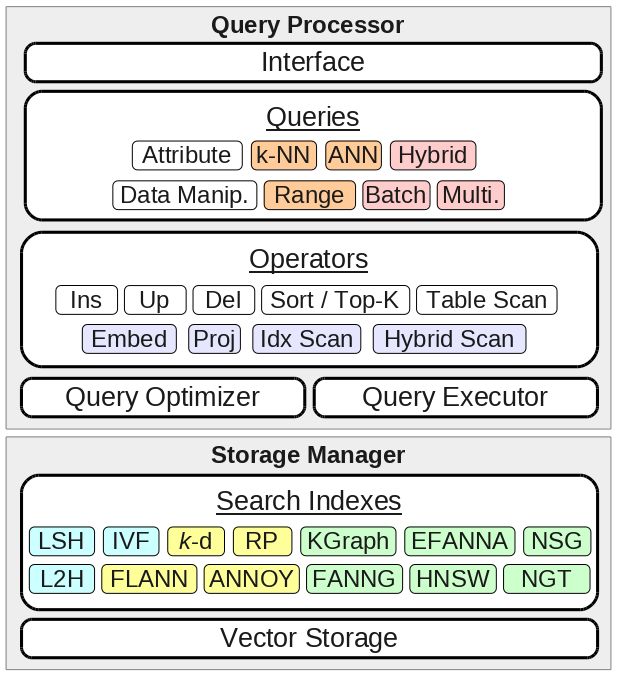
Consequently, the modules in a VDBMS split into a query processor, which includes the query specifications, logical operators, their physical implementations, and the query optimizer; and the storage manager, which maintains the search indexes and manages the physical storage of the vectors. This is illustrated in Figure 1.

The designs of these modules affect the runtime characteristics of the VDBMS. Many applications such as LLMs are read-heavy, requiring high query throughput and low latency. Others such as e-commerce are also write-heavy, requiring high write throughput. Additionally, some applications require high query accuracy, meaning that retrieved entities are true semantic matches to the query, while other applications may be more tolerant of errors. Developing a suitable VDBMS therefore requires understanding the landscape of techniques and how they affect characteristics of the system.

While there is mature understanding of processing conventional structured data, this is not the case for vector data. We present five key obstacles. (1) Vague Search Criteria. Structured queries use precise boolean predicates, but vector queries rely on a vague notion of semantic similarity that is hard to accurately capture. (2) Expensive Comparisons. Attribute predicates (e.g. $<$, $>$, $=$, and $\in$) can mostly be evaluated in $O(1)$ time, but a similarity comparison typically requires $O(D)$ time, where $D$ is the vector dimensionality. (3) Large Size. A structured query usually only accesses a small number of attributes, making it possible to design read-efficient storage structures such as column stores. But vector search requires full feature vectors. Vectors sometimes even span multiple data pages, making disk retrievals more expensive while also straining memory. (4) Lack of Structure. Structured attributes are mainly sortable or ordinal, leading to partitionings via numerical ranges or categories that can be used to design search indexes. But vectors have no obvious sort order nor are they ordinal, making it hard to design indexes that are both accurate and efficient. (5) Incompatibility with Attributes. Structured queries over multiple attribute indexes can use simple set operations, such as union or intersection, to collect the intermediate results into the final result set. But vector indexes typically stop after finding $k$ most similar vectors, and combining these with the results from an attribute index scan can lead to fewer than expected results. On the other hand, modifying the index scan operator to account for attribute predicates can degrade index performance. It remains unclear how to support “hybrid” queries over both attributes and vectors in a way that is both efficient and accurate.

There are now a variety of techniques that have been developed around these issues, aimed at achieving low query latency, high result quality, and high throughput while supporting large numbers of vectors. Some of these are results of decades of study on similarity search. Others, including hybrid query processing, indexes based on vector compression, techniques based on hardware acceleration, and distributed architectures are more recent inventions.

In this paper, we start by surveying these techniques from the perspective of a generic VDBMS, dividing them into those that apply to query processing and those that apply to storage and indexing. Query optimization and execution are treated separately from the core query processor. Following these discussions, we apply our understanding of these techniques to characterize existing VDBMSs.

Query Processing. The query processor mainly deals with how to specify the search criteria in the first place and how to execute search queries. For the former, a variety of similarity scores, query types, and query interfaces are available. For the latter, the basic operator is similarity projection, but as it can be inefficient, a variety of index-supported operators have been developed. We discuss the query processor in Section 2.

Storage and Indexing. The storage manager mainly deals with how to organize and store the vector collection to support efficient and accurate search. For most systems, this is achieved through vector search indexes. We classify indexes into table-based indexes such as E²LSH datar2004 , SPANN chen2021 , and IVFADC jegou2011product , that are generally easy to update; tree-based indexes such as FLANN muja2009 , RPTree dasgupta2008 ; dasgupta2013 , and ANNOY annoy that aim to provide logarithmic search; and graph-based indexes such as KGraph dong2011 , FANNG harwood2016 , and HNSW malkov2020 that have been shown to perform empirically well but with less theoretical understanding.

To address the difficulty of partitioning vector collections, techniques include randomization indyk1998 ; datar2004 ; andoni2015 ; muja2009 ; dasgupta2013 ; dong2011 ; wang2012 ; subramanya2019 , learned partitioning wang2018 ; jegou2011product ; matsui2018 ; muja2009 ; silpa2008 , and what we refer to as “navigable” partitioning dearholt1988 ; malkov2014 ; malkov2020 . To deal with large storage size, several techniques have been developed for indexes over compressed vectors, including quantization gray1984 ; jegou2011product ; matsui2018 ; sivic2003 ; wang2020 ; wei2020 , as well as disk-resident indexes gollapudi2023 ; chen2021 . We discuss indexing in Section 3.

Optimization and Execution. The query optimizer and executor mainly deals with plan enumeration, plan selection, and physical execution. To support hybrid queries, several hybrid operators have been developed, based on what we refer to as “block-first” scan wei2020 ; wang2021 ; gollapudi2023 and “visit-first” scan wu2022 . There are also several techniques for enumeration and selection, including rule-based and cost-based selection wei2020 ; wang2021 . For query execution, several techniques aim to exploit the storage locality of large vectors to design hardware accelerated operators, taking advantage of capabilities such as processor caches wang2021 , SIMD wang2021 ; andre2017 ; andre2021 , and GPUs johnson2021 . There are also distributed search techniques and techniques for supporting high throughput updates, namely based on out-of-place updates. We discuss optimization and execution in Section 4.

Current Systems. We classify existing VDBMSs into native systems which are designed specifically around vector management, including Vearch li2018 , Milvus wang2021 , and Manu guo2022 ; extended systems which add vector capabilities on top of an existing data management system, including AnalyticDB-V wei2020 and PASE yang2020 ; and search engines and libraries which aim to provide search capability only, such as Apache Lucene lucene , Elasticsearch elastic , and Meta Faiss faiss . Native systems tend to favor high performance techniques targeted at specific capabilities, while extended systems tend to favor techniques that are more adaptable to different workloads but are not necessarily the fastest. We survey current systems in Section 5.

Related Surveys. A high level survey is available that mostly focuses on fundamental VDBMS concepts and use cases. Likewise, some tutorials are available that focus specifically on similarity search qin2020 ; qin2021 . We complement these by focusing on specific problems and techniques related to vector data management as a whole. Surveys are also available covering data types that are related to vectors, such as time series and strings, but not supported by VDBMSs. Unlike systems for these other data types, a VDBMS can make no assumptions about feature vector dimensions. We refer readers to echihabi2019 ; echihabi2021 .

For the remaining sections, we briefly discuss benchmarks in Section 6, followed by a summary of research challenges and open problems in Section 7. We conclude the survey in Section 8.

2 Query Processing

Query processing in a VDBMS begins with a search specification consisting of the similarity score and the query type. Search criteria are conveyed to the system through a query interface. Once a query is received by the system, it is processed by executing a chain of operators over the vector collection.

2.1 Similarity Scores

A similarity score $f:\mathbb{R}^{D}\times\mathbb{R}^{D}\rightarrow\mathbb{R}$ maps two $D$-dimensional vectors, $\mathbf{a}$ and $\mathbf{b}$, onto a scalar, $f(\mathbf{a},\mathbf{b})$, with larger values indicating greater similarity.

Similarity is often measured via distance in practice, with values closer to $0$ indicating greater similarity. Distance functions obey the metric axioms of identity ($d(\mathbf{a},\mathbf{a})=0$), positivity ($d(\mathbf{a},\mathbf{b})>0\textrm{ if }\mathbf{a}\neq\mathbf{b}$), symmetry ($d(\mathbf{a},\mathbf{b})=d(\mathbf{b},\mathbf{a})$), and triangle inequality ($d(\mathbf{a},\mathbf{c})\leq d(\mathbf{a},\mathbf{b})+d(\mathbf{b},\mathbf{c})$ for any three vectors $\mathbf{a},\mathbf{b},\mathbf{c}$). Several similarity scores are commonly supported by VDBMSs, and these are summarized in Table 1.

Aside from these basic scores, some VDBMSs also support aggregate scores for applications like multi-vector search wang2020 . There is also emerging work on learned scores abdelkader2019 ; zhang2020 ; meng2022 , but these are not available in commercial systems.

Table 1: Common similarity scores.

Type	Score	Metric	Complexity	Range
Sim.	Inner Prod.	✗	$O(D)$	$\mathbb{R}$
	Cosine	✗	$O(D)$	$\left[-1,1\right]$
Dist.	Minkowski	✓	$O(D)$	$\mathbb{R}^{+}$
	Mahalanobis	✓	$O(D^{2+O(1)})$	$\mathbb{R}^{+}$
	Hamming	✓	$O(D)$	$\mathbb{N}$

2.1.1 Basic Scores

The Hamming distance counts the number of differing dimensions between vectors $\mathbf{a}$ and $\mathbf{b}$.

Definition 1 (Hamming)

$d(\mathbf{a},\mathbf{b})=\sum_{i=1}^{n}\delta_{a_{i}b_{i}}$

where $\delta$ is the Kronecker delta.

Other similarity scores start from an inner product. For $\mathbb{R}^{D}$ space, the dot product typically serves as the inner product.

Definition 2 (Inner Product)

$f(\mathbf{a},\mathbf{b})=\sum_{i=1}^{n}a_{i}b_{i}$,

also written $f(\mathbf{a},\mathbf{b})=\langle\mathbf{a},\mathbf{b}\rangle=\mathbf{a}\cdot\mathbf{b}$. The quantity $\sqrt{\langle\mathbf{a},\mathbf{a}\rangle}$ defines the Euclidean norm $\lVert\mathbf{a}\rVert$ or magnitude of $\mathbf{a}$. Euclidean distance is the norm of the vector resulting from the subtraction of two vectors, $\lVert\mathbf{a}-\mathbf{b}\rVert$. Euclidean distance is metric.

The dot product projects $\mathbf{a}$ onto $\mathbf{b}$ and scales the result by the magnitude of $\mathbf{b}$. The scaling can lead to unintuitive consequences. For example, two large identical vectors have a larger dot product compared to two small identical vectors, thus they would be considered “more similar” under this definition.

If magnitude is not important, $\mathbf{a}$ and $\mathbf{b}$ can be normalized by $\mathbf{\hat{a}}=\mathbf{a}/\lVert\mathbf{a}\rVert$ and $\mathbf{\hat{b}}=\mathbf{b}/\lVert\mathbf{b}\rVert$ so that they possess unit magnitudes. Then,

Definition 3 (Cosine Similarity)

$f(\mathbf{a},\mathbf{b})=\langle\mathbf{\hat{a}},\mathbf{\hat{b}}\rangle$

or $f(\mathbf{a},\mathbf{b})=\frac{\langle\mathbf{a},\mathbf{b}\rangle}{\lVert\mathbf{a}\rVert\lVert\mathbf{b}\rVert}$. Cosine similarity yields the angle between $\mathbf{a}$ and $\mathbf{b}$.

Arbitrary $p$-norms, $\lVert\mathbf{x}\rVert_{p}=(|x_{1}|^{p}\dots|x_{D}|^{p})^{1/p}$, induce the Minkowski distance, generalizing Euclidean distance.

Definition 4 (Minkowski)

The $p$-order Minkowski distance is $d(\mathbf{a},\mathbf{b})=(\sum_{i=1}^{n}|a_{i}-b_{i}|^{p})^{1/p}$,

or $d(\mathbf{a},\mathbf{b})=\lVert\mathbf{a}-\mathbf{b}\rVert_{p}$. All positive and integer values of $p$ yield metrics.

Another generalization of Euclidean distance can be obtained by applying a linear transformation over the vector space in order to adjust the relative proximities of the feature vectors. The distance of two vectors in the transformed space can be calculated using the Mahalanobis formula.

Definition 5 (Mahalanobis)

For any positive semi-definite matrix $\mathsf{M}$, $d(\mathbf{a},\mathbf{b})=\sqrt{(\mathbf{a}-\mathbf{b})^{\top}\mathsf{M}(\mathbf{a}-\mathbf{b})}$.

2.1.2 Aggregate Scores

Sometimes, a single real-world entity is represented by multiple vectors in the vector collection. For example for facial recognition, a face may be represented by multiple images taken from different angles, leading to $m$ feature vectors $\mathbf{x}_{1}\dots\mathbf{x}_{m}$.

Given a query vector $\mathbf{q}$, finding the set of vectors which are collectively most similar to $\mathbf{q}$ is called multi-vector search. One way of approaching this problem is to use an aggregate score that defines how to combine individual scores $f(\mathbf{x}_{1},\mathbf{q})\dots f(\mathbf{x}_{m},\mathbf{q})$ to yield a single value that can be compared. Examples are the mean aggregate $1/m\sum_{i=1}^{m}f(\mathbf{x}_{i},\mathbf{q})$ and the weighted sum wang2021 .

2.1.3 Learned Scores

Some recent works abdelkader2019 ; zhang2020 ; meng2022 aim to find a transformation, $\mathsf{M}$, in order to improve the quality of similarity search over Mahalanobis distance. Finding $\mathsf{M}$ is one of the goals of metric learning, and we point interested readers to wang2015 for a survey of techniques.

2.1.4 Discussion

Score Selection. Many scores have been proposed over the years, but how to select an appropriate score for a particular application remains unclear. Ideally, a score is selected so that query answers accurately reflect the true semantic similarities between real-world entities represented by the vectors. But so far, there are no principles guiding score selection, and as a result, score selection tends to be based more on informal rules distilled from experience rather than on rigorous theory.

Many VDBMSs offer this as a choice to the user, and how to support automatic score selection remains an open problem. We are aware of one recent work wang2023 that dynamically adjusts the score based on the query for social media content recommendation.

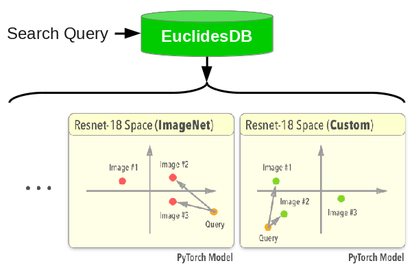
At a higher level, vector search is affected not only by the similarity score but also by the nature of the embeddings and the semantics of the query. A preliminary discussion on query semantics is given in tagliabue2023 . Hence, we imagine that future solutions will be more holistic, considering this problem from all aspects beyond score selection. For example, EuclidesDB euclid allows users to conduct the same search but over multiple embedding models and scores in order to identify the most semantically meaningful settings.

Curse of Dimensionality. When $D$ grows beyond around 10 dimensions, and when the dimensions are independent and identically distributed, the Euclidean distances between the two farthest and two nearest vectors approach equality as the variance nears zero beyer1999 . The effect of this “curse of dimensionality” is that vectors become indiscernible.

Attempts at avoiding the curse have led to using other Minkowski distances, such as the Manhattan distance ($p=1$) or the Chebyshev distance ($p=\infty$), in an effort to recover discernability aggarwal2001 . Fractional orders of $p<1$ have also been explored mirkes2020 but so far, results are inconclusive.

2.2 Queries and Operators

Let $S\subset\mathbb{R}^{D}$ be a vector collection with $N$ members. Let $\mathbf{q}$ be a $D$-dimensional query vector which may or may not belong to $S$.

Data manipulation queries aim to modify $S$. Given $S$, $\mathbf{q}$, and a way to measure similarity (whether by $f$ or $d$), vector search queries aim to return a subset of $S$ where each member of the subset satisfies criteria based on similarity to $\mathbf{q}$. Different criteria lead to different types of queries.

To answer these queries, a VDBMS may use several basic operators in addition to more sophisticated index operators that will be discussed in Section 3.

2.2.1 Data Manipulation Queries

Data manipulation queries provide insert, update, and delete mechanisms over $S$. In a traditional data management system, data is manipulated directly. But in a VDBMSs, feature vectors are proxies for the actual entities, and they can be manipulated either directly or indirectly. An embedding model maps real-world entities (e.g. images) to feature vectors.

Under direct manipulation, users freely manipulate the values of the vectors, and maintaining the model is the responsibility of the user. This is the case for systems such as PASE yang2020 and pgvector pgvec .

For indirect manipulation, vectors are hidden from users. The vector collection appears as a collection of entities, not vectors, and users manipulate the entities. The VDBMS is responsible for the model, which can be user-provided, for example through a user-defined function (UDF) as in Vald vald , or selected from a menu of pre-trained models. For example, Pinecone pine supports a large number of pre-trained *2vec models by connecting to special providers via REST API.

There is extensive literature on designing embedding models, and we refer interested readers to pouyanfar2018 .

2.2.2 Basic Search Queries

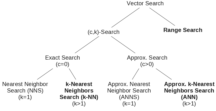
Several types of search queries exist, but not all VDBMSs support all types. The queries are shown in Figure 2.

Figure 2: Basic search queries.

Search queries can be viewed as either similarity maximization or distance minimization with respect to $\mathbf{q}$. We take the latter for the following definitions.

$(c,k)$-Search Queries. Most VDBMSs support “nearest neighbor” queries, where the aim is to retrieve vectors from $S$ that are physical neighbors of $\mathbf{q}$ in the vector space. These queries may aim to return exact or approximate nearest neighbors, and may also specify the number of neighbors to return. We refer to these as $(c,k)$-search queries, where $c$ indicates the approximation degree and $k$ is the number of neighbors.

Out of these, most VDBMSs support the approximate $k$-nearest neighbors (ANN) query, which returns $k$ vectors from $S$ that are within a radius, centered over $\mathbf{q}$, of $c$ times the distance between $\mathbf{q}$ and its closest neighbor.

Definition 6 (ANN)

Find a $k$-size subset $S^{\prime}\subseteq S$ such that $d(\mathbf{x}^{\prime},\mathbf{q})\leq c(\min_{\mathbf{x}\in S}d(\mathbf{x},\mathbf{q}))$ for all $\mathbf{x}^{\prime}\in S^{\prime}$.

If $k=1$, we call this query approximate nearest neighbor search (ANNS).

When $c=1$, we call this an exact query. The case $c=1,k=1$ corresponds to nearest neighbor search (NNS) (see Note 7), and when $c=1,k>1$, the query is called a $k$-nearest neighbors ($k$-NN) query.

We note that there is a large literature on the maximum inner product search (MIPS) problem, which is the NNS query but over inner products. We refer interested readers to teflioudi2016 for an overview.

Range Queries. A range query is parameterized by a radius, $r$, instead of the number of neighbors to return.

Definition 7 (Range)

Find $\{\mathbf{x}\in S\mid d(\mathbf{x},\mathbf{q})\leq r\}$.

2.2.3 Query Variants

Some VDBMSs support variations on these basic query types, listed in Table 2.

Table 2: Query variants.

Variant	Sub-Variant
Predicated
Batched
Multi-Vector	Multi-Query, Single Feature (MQSF)
	Multi-Query, Multi-Feature (MQMF)
	Single-Query, Multi-Feature (SQMF)

Predicated Search Queries. In a predicated search query, or “hybrid” query, each vector is associated with a set of attribute values, and a boolean predicate over these values must evaluate to true for each record in the result set. Here is an example:

Example 1

A hybrid $k$-NN query written in SQL is:

In this example, d is a distance function parameterized by the query q, and every member of the result set must satisfy the conditions of being among the k nearest and of obeying the predicate, attr < c.

Batched Queries. For batched queries, a number of queries are revealed to the system at the same time, and the VDBMS can answer them in any order.

These queries are especially suited to hardware accelerated query processing wang2021 ; johnson2021 .

Multi-Vector Queries. Some VDBMSs also support multi-vector search queries via aggregate scores.

There are three possible sub-types: in multi-query single-feature (MQSF) queries, the query is represented by multiple vectors, and real-world entities are represented by single feature vectors; in multi-query multi-feature (MQMF) queries, both the query and the entities are represented by multiple vectors; and in single-query multi-feature (SQMF) queries, only the entities are represented by multiple vectors. But so far, there is support for MQSF and SQMF queries marqo ; weaviate ; milvus ; wang2021 ; nuclia but no support for MQMF queries.

2.2.4 Basic Operators

It is possible to answer all $(c,k)$-search and range queries using only projection.

Definition 8 (Projection)

The projection of $S$ onto $g$ under query $\mathbf{q}$ yields $\pi_{g}(S)=\{g(\mathbf{x},\mathbf{q})\mid\mathbf{x}\in S\}$.

Projection onto $g=f$ or $g=d$ alone is sufficient for vector search queries by projecting the full collection in time $O(\tau N)$, where $\tau$ is the cost of $g$.

Typically $\tau$ is in $O(D)$, making projection by itself impractical for VDBMSs where $N$ and $D$ are very large. Thus, most VDBMSs rely on specialized index-based operators in addition to projection.

2.2.5 Discussion

Query Accuracy and Performance. The search capability of a VDBMS is assessed by evaluating query accuracy and performance.

To evaluate accuracy, precision and recall are often used. Precision is defined as the ratio between the number of relevant results in the result set over the size of the result set, and recall is defined as the ratio between the number of retrieved relevant results over all possible relevant results. For example in a $k$-NN query, the precision is $k^{\prime}/|S^{\prime}|$, where $k^{\prime}$ is the number of true nearest neighbors in $S^{\prime}$, and the recall is $k^{\prime}/k$.

To evaluate performance, latency and throughput are used. Latency is the amount of time it takes for a VDBMS to answer a query once it is received, while throughput is the number of queries that are answered per unit time, often reported as queries per second.

Theoretical Results. Similarity search has a long history, making it possible to summarize some key theoretical results. For low-dimensional NNS, many theoretical results are known. Algorithms with $O(\log N)$ query times and $O(N)$ storage are known for $D=1$ (e.g. binary search trees) and $D=2$ lipton1980 . For the latter case, $k$-d trees bentley1975 are particularly well known, and the query complexity is $O(\sqrt{N})$. For $D\geq 3$, sub-linear search performance is much harder to obtain. In the general case, $k$-d trees offer $O(DN^{1-1/D})$ query complexity lee1977 , which tends toward $O(DN)$ as $D$ grows. On the other hand, meiser1993 offers $O(D^{O(1)}\log N)$ query complexity but requires super-polynomial $O(N^{O(D)})$ storage. The modern belief is that even a fractional power of $N$ query complexity cannot be obtained unless storage cost is worse than $N^{O(1)}D^{O(1)}$ andoni2018 ; rubinstein2018 .

Locality sensitive hashing (LSH) indyk1998 is perhaps the most well understood ANN algorithm. The query complexity is dominated by $N^{\rho}$ while the storage complexity is dominated by $N^{1+\rho}$, where $0\leq\rho\leq 1$. Recently, heuristic methods which lack guarantees have become popular. There are encouraging analyses of graph-based techniques laarhoven2018 ; prokhorenkova2020 but these lack the maturity of LSH.

2.3 Query Interfaces

For query interfaces, native and NoSQL VDBMSs tend to rely on small APIs. For example, Chroma chroma offers a Python API with just nine commands, including add, update, delete, and query.

On the other hand, extended VDBMSs built over relational systems tend to take advantage of SQL extensions. In pgvector pgvec , a $k$-NN or ANN query is expressed as:

The syntax R <-> s returns the Euclidean distance between all the tuples of R and vector s, and other distance functions are supported via other symbols. If an ANN index is created over the items table, then this query will return approximate results if the index is used for execution.

Similarly, range queries are expressed using where:

3 Indexing

While all $(c,k)$-search and range queries can be answered by comparing $\mathbf{q}$ with each of the $N$ vectors, the complexity of this brute-force approach is $O(DN)$, prohibitive for large $D$ and $N$.

Instead, vector indexes speed up queries by minimizing the number of comparisons. This is achieved by partitioning $S$ so that only a small subset is compared, and then arranging the partitions into data structures that can be easily traversed.

Unlike typical attributes, vectors are not obviously sortable nor can they be easily categorized. To achieve high accuracy, these indexes rely on novel techniques which we refer to as randomization, learned partitioning, and navigable partitioning. The large physical size of vectors also leads to use of compression, namely a technique called quantization, as well as disk resident designs. Additionally, the need to support predicated queries has led to special hybrid operators for indexes, which we will discuss in Section 4.

Partitioning Techniques.

• Randomization. Randomization aims to exploit probability amplification of multiple independent events, allowing indexes to better discriminate truly similar vectors from dissimilar ones.

• Learned Partitioning. Learning-based techniques aim to uncover an internal structure of $S$ so that it can be partitioned along this structure. These techniques can be supervised or unsupervised.

• Navigable Partitioning. Instead of fixating on absolute partitions, navigable indexes are designed so that different regions of $S$ can be easily traversed.

Some partitioning strategies are data independent, where the rules are the same for any data distribution. But the majority are data dependent. If updates to $S$ alter its distribution, then indexes based on data dependent strategies may eventually become unbalanced over time. In many cases, this can only be resolved by rebuilding the index.

Storage Techniques.

• Quantization. A quantizer maps a vector onto a more space-efficient representation. Quantization is usually lossy, and the aim is to minimize information loss while simultaneously minimizing storage cost.

• Disk-Resident Designs. Compared to memory resident indexes which only minimize the number of comparisons, disk resident indexes additionally aim to minimize the number of retrievals.

Below, we examine the main techniques for some common indexes. One particular index may use a combination of techniques, and so we classify indexes based on their structure and then point out which techniques are used in which index. There are three basic structures: tables divide $S$ into buckets containing similar vectors; trees are a nesting of tables; graphs connect similar vectors with virtual edges that can then be traversed. All of these structures are capable of achieving high query accuracy but with different construction, search, and maintenance characteristics.

3.1 Tables

Table 3: Representative table-based indexes.

Type	Index	Hash Function
LSH	E2LSH datar2004	Rand. hyperplanes
	IndexLSH	Rand. bits
	FALCONN andoni2015	Rand. balls
L2H	SPANN chen2021	Nearest centroid
Quant.	SQ	Nearest discrete value
	PQ	Nearest centroid product
	IVFSQ	Nearest centroid
	IVFADC jegou2011product	Nearest centroid

The main consideration for table-based indexes is the design of the bucketing hash function. The most popular table-based indexes for VDBMSs tend to use randomization and learned partitions, as shown in Table 3. For randomization, techniques based on LSH andoni2008 ; andoni2015 ; andoni2018 ; datar2004 ; indyk1998 ; leskovec2014 ; lv2007 are popular due to robust error bounds. For learned partitions, learning-to-hash (L2H) wang2018 directly learns the hash function, and indexes based on quantization gray1984 ; jegou2011product ; matsui2018 ; sivic2003 ; wang2020 ; wei2020 typically uses $k$-means berg2008 to learn geometric clusters of similar vectors.

All of these indexes have similar construction and search characteristics. For construction, each vector is hashed into one of the buckets. The total complexity is typically $O(DN^{1+\epsilon})$, $0\leq\epsilon\leq 1$. For LSH, each vector is hashed multiple times, leading to $\epsilon>0$. For quantization-based approaches, $k$-means multiplies the complexity by a constant factor. For search, $\mathbf{q}$ is hashed onto a key and then the corresponding bucket is scanned. Hashing is generally on the order of $O(D)$. Usually only a small fraction of $S$ is scanned, yielding a complexity of about $O(DN^{\epsilon})$, including the cost of hashing and bucket scan.

3.1.1 Locality Sensitive Hashing

Locality sensitive hashing indyk1998 ; leskovec2014 provides tunable performance with error guarantees, but it can require high redundancy in order to boost accuracy, increasing query and storage costs relative to other techniques.

In a “family” of hash functions $H=\{h:S\rightarrow U\}$, if $d(\mathbf{x},\mathbf{q})\leq r_{1}$, then $\Pr_{H}(h(\mathbf{x})=h(\mathbf{q}))\geq p_{1}$, and if $d(\mathbf{x},\mathbf{q})\geq r_{2}$, then $\Pr_{H}(h(\mathbf{x})=h(\mathbf{q}))\leq p_{2}$, for any $r_{1}$, $r_{2}$, $\mathbf{x}\in S$, and $\mathbf{q}$. A tunable family $G=\{g:S\rightarrow U^{K}\}$ is derived by letting $g(\mathbf{x})$ return the concatenation of $h_{i}(\mathbf{x})$ for $i$ between $1$ and some constant $K$.

The table is constructed by hashing each $\mathbf{x}\in S$ into each of the $L$ hash tables using $g_{1}\dots g_{L}$. Typically, $L$ is set to $L=O(1/p_{1}^{K})$ with $K$ set to $\lceil\log_{1/p_{2}}N\rceil$ andoni2018 . The exact value depends on the accuracy and performance needs of the application, and some sample curves are shown in andoni2008 . Letting $\rho=\log(1/p_{1})/\log(1/p_{2})$ yields $L=O(N^{\rho}/p_{1})$. The storage complexity is $O(LDN)$ which is $O(DN^{1+\rho})$ after substitution. In the practical case where $p_{1}>p_{2}$, the value of $\rho$ is between $0$ and $1$.

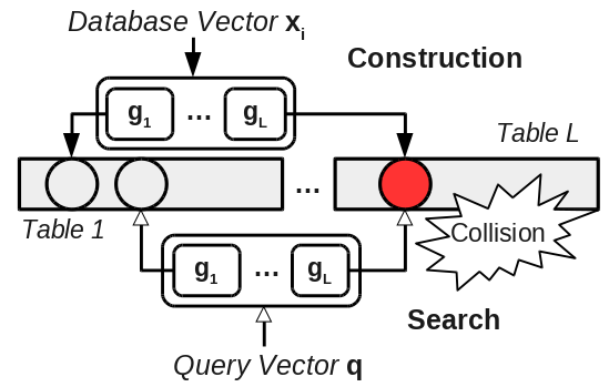
When a query appears, it is hashed using the $L$ hash functions sampled from $G$, and collisions are kept as candidate neighbors. The candidates are then re-ranked or discarded based on true distances to $\mathbf{q}$. Figure 3 illustrates this procedure. The query complexity is dominated by the $L$ hash evaluations, which is $O(DN^{\rho})$.

When $r_{1}$ is set to $\min_{\mathbf{x}\in S}d(\mathbf{x},\mathbf{q})$ and $r_{2}$ is set to $cr_{1}$, the $c$ guarantee is relative to the minimum distance. This is useful when the query is static across the workload, but is is hard to generalize over dynamic online queries. Hence for an index designed around some given hash family, not all queries may have similar candidate sets, making it hard to control precision and recall. Multi-probe LSH lv2007 is one attempt at addressing this issue by scanning multiple buckets at a time, thereby spreading out the search.

Figure 3: Constructing and searching an LSH index.

We mention a few popular LSH schemes. The first two are data independent and require no rebalancing.

• E²LSH. Each $g$ is an $O(D)$ projection onto a random hyperplane. This achieves $\rho<1/c$ datar2004 .

• IndexLSH. This scheme is based on binary projections and is provided by Faiss faiss .

There have also been efforts at designing data dependent hash families to yield lower $\rho$.

• FALCONN. Implements an LSH hash family based on spherical LSH andoni2015 . The dataset is first projected onto a unit ball and then recursively partitioned into small overlapping spheres. The $\rho$ value is $1/(2c^{2}-1)$.

Other families are given in andoni2018 .

3.1.2 Learning to Hash

Learning-based techniques aim to directly learn suitable mappings without resorting to hash families. For example, spectral hashing weiss2008 designs hash functions based on the principal components of the similarity matrix of $S$. In salakhutdinov2007 , hash functions are modeled using neural networks. In SPANN chen2021 , vectors are hashed to the nearest centroid following $k$-means. Several techniques for a disk resident table-based index are also given.

These techniques tend to require lengthy training and are sensitive to out-of-distribution updates, and they are not widely supported in VDBMSs. We point readers to wang2018 for a survey of techniques.

3.1.3 Quantization

One of the main criticisms of LSH is that the storage cost can be large due to the use of multiple hash tables. For in-memory VDBMSs, large memory requirements can be impractical. While some efforts aim at reducing these storage costs zhang2016 , other efforts have targeted vector compression using quantization gray1984 ; sivic2003 ; jegou2011product .

Many of these techniques use $k$-means centroids as hash keys. A large $K$ number of centroids can modulate the chance of collisions, keeping buckets reasonably small and speeding up search. Normally, $k$-means is terminated once a locally optimal set of centroids is found, with complexity $O(DN\cdot K)$ per iteration.

Figure 4: In this example from wang2020 , each 4-dimensional vector is divided into two 2-dimensional sub-spaces.

But large $K$ make $k$-means expensive. Product quantization exploits the fact that the cross product of $m$ number of $(D/m)$-dimensional spaces is a space of $D$ dimensions, so that by setting $U=\prod_{j=1}^{m}U_{i}$, then $U\in\mathbb{R}^{D}$ when $U_{j}\in\mathbb{R}^{D/m}$. This means that to yield a count of $K$ centroids, only $K^{1/m}$ centroids need to be found per $U_{j}$. Moreover as each $U_{j}$ belongs to a lower dimensional space, the running time of $k$-means per $U_{j}$ is reduced. The new complexity is $O(m)O(\frac{D}{m}NK^{1/m}i)$.

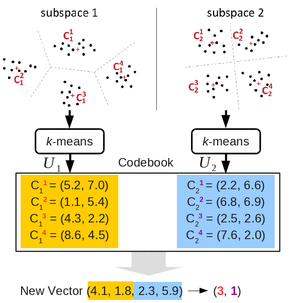
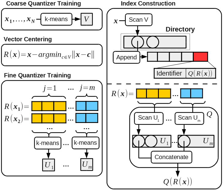
Each $U_{j}$ is constructed via $k$-means over the collection of sub-vectors $\{(x_{i})^{jD/m}_{i=(j-1)D/m+1}\mid\mathbf{x}\in S\}$, and the set of all $U_{j}$ is known as the “codebook”. Vector $\mathbf{x}$ is then quantized by splitting it into $m$ sub-vectors, $\mathbf{x}^{\prime}_{j}$, finding the nearest centroid in $U_{j}$ to $\mathbf{x}^{\prime}_{j}$ for each $j\in 1\dots m$, and then concatenating these centroids. Each vector is thus stored using $m\log_{2}(D/m)$ bits, and the time complexity is $O(m)O(DK^{1/m})$. An example is shown in Figure 4.

Various techniques such as Cartesian $k$-means norouzi2013 , optimized PQ (OPQ) ge2013 , hierarchical quantizers yandex2016 , and anisotropic quantizers guo2020 have been developed based on this idea, offering around 60% better recall in the best cases at the cost of additional processing. A survey of these techniques is given in matsui2018 . The storage cost can also be reduced by constant factors wang2020 .

Figure 5: Construction of an IVFADC index.

We list some quantization-based indexes.

• Flat Indexes. Faiss faiss supports a number of “flat” indexes where each vector is directly mapped onto its compressed version, without any bucketing. The standard quantizer index, SQ, performs a bit-level compression, for instance by mapping 64-bit doubles onto 32-bit floats. The PQ index directly maps each vector onto its PQ code.

• IVFSQ. For IVFSQ, the vectors are compressed using SQ and bucketed to their nearest centroid.

• IVFADC. Training a PQ quantizer over $S$ can still be time consuming. To reduce this cost, IVFADC first buckets vectors using $k$-means over a small number of centroids, and then trains a PQ quantizer by sampling a few vectors from each of the buckets. To allow a single quantizer to apply to all the buckets, each vector $\mathbf{x}$ is normalized by subtracting from its bucket key, resulting in a “residual” vector $R(\mathbf{x})$ which is then used to train the quantizer. The full workflow is shown in Figure 5. During search, query $\mathbf{q}$ is directly compared against the quantized vectors in the bucket that $\mathbf{q}$ maps onto. As $\mathbf{q}$ itself is not quantized, the comparison is referred to as an “asymmetric distance computation” (ADC).

For IVFADC, many distance calculations are likely to be repeated during bucket scan since many vectors may share the same PQ centroids. These calculations can be avoided by first computing $\lVert\overline{\mathbf{q}_{j}}-\mathbf{c}\rVert^{2}$ for all $\mathbf{c}\in U_{j}$ and for all $j\in 1\dots m$, where $\overline{\mathbf{q}_{j}}$ is the $j$th sub-vector of $\mathbf{q}$ matsui2018 . This preprocessing step takes $O(m)O(\frac{D}{m}K^{\prime})$, where $K^{\prime}$ is the number of centroids in $U_{j}$. But afterwards, ADC can be performed using just $m$ look-ups, reducing bucket scan from $O(DN)$ to $O(mN)$.

Example 2

Below is the ADC look-up table when $U$ is divided into $m$ subsets, and where each subset contains $K^{\prime}$ centroids. Here, $\overline{\mathbf{q}_{j}}$ is the $j$th sub-vector of query $\mathbf{q}$, and $\mathbf{c}^{j}_{i}$ is the $i$th centroid in the $j$th subset of $U$.

$$\overbrace{\begin{matrix}d(\overline{\mathbf{q}_{1}},\mathbf{c}^{1}_{1})&\cdots&d(\overline{\mathbf{q}_{1}},\mathbf{c}^{1}_{K^{\prime}})\\ \vdots&\ddots&\vdots\\ d(\overline{\mathbf{q}_{m}},\mathbf{c}^{1}_{1})&\cdots&d(\overline{\mathbf{q}_{m}},\mathbf{c}^{1}_{K^{\prime}})\end{matrix}}^{U_{1}},\cdots,\overbrace{\begin{matrix}d(\overline{\mathbf{q}_{1}},\mathbf{c}^{m}_{1})&\cdots&d(\overline{\mathbf{q}_{1}},\mathbf{c}^{m}_{K^{\prime}})\\ \vdots&\ddots&\vdots\\ d(\overline{\mathbf{q}_{m}},\mathbf{c}^{m}_{1})&\cdots&d(\overline{\mathbf{q}_{m}},\mathbf{c}^{m}_{K^{\prime}})\end{matrix}}^{U_{m}}$$

We mention one other technique. In AnalyticDB-V wei2020 , each bucket is further divided into finer sub-buckets in order to avoid accessing multiple full buckets. The resulting structure is called a “Voronoi Graph Product Quantization” (VGPQ) index.

3.2 Trees

For tree-based indexes, the main consideration is the design of the splitting strategy used to recursively split $S$ into a search tree.

A natural approach is to split based on distance. The main techniques includes pivot-based trees chen2022 ; chen2022survey , such as VP-tree yianilos1993 and M-tree ciaccia1997 , $k$-means trees muja2009 , and trees based on deep learning li2023 . Other basic techniques are described in sellis1997 . But while these trees are effective for low $D$, they suffer from the curse of dimensionality when applied to higher dimensions.

High-$D$ tree-based indexes tend to rely on randomization for performing node splits. In particular, “Fast Library for ANN” (FLANN) flann ; muja2009 combines randomization with learned partitioning via principal component analysis (PCA), extending the PKD-tree technique from silpa2008 , and “ANN Oh Yeah” (ANNOY) annoy is similar to the random projections tree (RPTree) from dasgupta2008 ; dasgupta2013 . These trees are summarized in Table 4.

The generic tree construction algorithm, from dasgupta2008 , is restated below:

procedure MakeTree($S$)

     if $|S|\leq\tau$ then return Leaf

     end if

     $\text{Rule}\leftarrow\text{ChooseRule}(S)$

     $\text{LeftTree}\leftarrow\text{MakeTree}(\{\mathbf{x}\in S\mid\text{Rule}(\mathbf{x})\text{ is true}\})$

     $\text{RightTree}\leftarrow\text{MakeTree}(\{\mathbf{x}\in S\mid\text{Rule}(\mathbf{x})\text{ is false}\})$

     return $(\text{Rule},\text{LeftTree},\text{RightTree})$

end procedure

The complexity is characteristically $O(DN\log N)$, ignoring any preprocessing costs. More precise bounds for several trees are given in ram2019 .

Most trees are able to return exact query results by performing backtracking, where neighboring leaf nodes are also checked during the search. However, this is inefficient weber1998 , and they are more often used for returning approximate results using defeatist search dasgupta2013 . In this procedure, the tree is traversed down to the leaf level, and all vectors within the leaf covering $\mathbf{q}$ are returned immediately as the nearest neighbors. There is no backtracking, and the complexity is $O(D\log N)$.

For maintenance, insertions require $O(D\log N)$ on average and $O(DN)$ in the worst case. But as node splits are determined during construction, there is no obvious way to rebalance the nodes after a number of out-of-distribution insertions. Self-balancing trees exist for scalar data adelson1962 but not for high-dimensional vectors.

Table 4: Representative tree-based indexes.

Index	Splitting Plane	Splitting Point
$k$-d tree bentley1975	Axis parallel	Median
PKD-tree silpa2008	Principal dim.	Median
FLANN muja2009	Random principal dim.	Median
RPTree dasgupta2008 ; dasgupta2013	Random plane	Median + offset
ANNOY annoy	Random plane	Random median

3.2.1 Non-Random Trees

Many high-$D$ trees derive from $k$-d tree, which splits along medians while rotating through dimensions:

procedure ChooseRule($S$)

     $i\leftarrow l\mod D$ where $l$ is the current depth

     $\text{Rule}\coloneqq(x_{i}\leq\text{median}(\{y_{i}\mid\mathbf{y}\in S\}))$

     return Rule

end procedure

This rule has the effect of fixing the splitting planes parallel to the dimensional axes dasgupta2008 ; ram2019 .

3.2.2 Random Trees

If certain dimensions explain the variance more than others, then the intrinsic dimensionality is lower than $D$. But in this case, $k$-d tree is unable to partition along these dimensions, leaving it susceptible to the curse of dimensionality. This limitation has led to the discovery of more adaptive splitting strategies.

Principal Component Trees. A principal component tree is a $k$-d tree that is constructed by first rotating $S$ so that the axes are aligned with the principal components of $S$. The principal dimensions need to be found beforehand using principal component analysis (PCA). The complexity of this step is $O(D^{2}N+D^{3})$.

• PKD-tree. In PKD-tree, the splitting plane is selected by rotating through the principal dimensions, similar to in vanilla $k$-d tree silpa2008 .

• FLANN. Instead of rotating through the dimensions, FLANN muja2009 splits along random principal dimensions.

Random Projection Trees. On the other hand, random splitting planes can be used to adapt to the intrinsic dimensionality without expensive PCA.

• RPTree. RPTree dasgupta2008 ; dasgupta2013 extends the idea of randomly rotated trees explored in vempala2012 by introducing random splits in addition to random splitting planes. The principle follows from spill trees liu2004 , where partitions are allowed to overlap. In RPTree, perturbed median splits simulate the effects of overlapping splits but with less storage cost. The splitting rule is dasgupta2013 :

  procedure ChooseRule($S$)

       $\mathbf{u}\leftarrow\text{A vector from the unit sphere}$

       $\beta\leftarrow\text{A number from }[0.25,0.75]$

       $v\leftarrow\text{The }\beta\text{ fractile of }\pi_{\mathbf{u}}(S)$

       $\text{Rule}\coloneqq(\mathbf{x}\cdot\mathbf{u}\leq v)$

       return Rule

  end procedure

  The values of $\mathbf{u}$, $\beta$, and $\mathbf{v}$ are uniformly chosen at random. The operation $\pi_{\mathbf{u}}(S)$ performs a projection of $S$ onto $\mathbf{u}$. Variable $v$ represents the perturbed median split, with $\beta=0.5$ yielding the true median.

• ANNOY. Instead of splitting on the $\beta$ fractile, ANNOY splits along the median of two random values sampled from $\pi_{\mathbf{u}}(S)$, which is simpler to compute.

Several theoretical results are known for RPTree, but it is not clear if these apply to ANNOY.

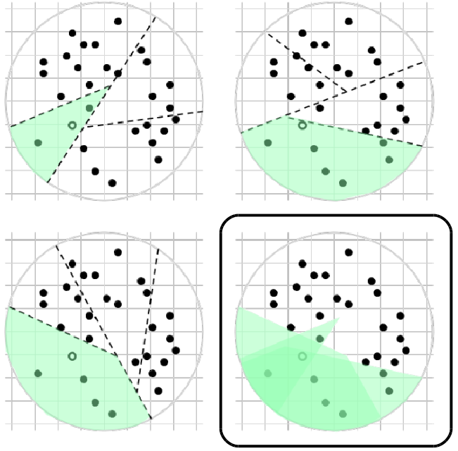
As shown in Figure 6, a forest of random trees can be used to improve recall. We mention that RPTree incurs a storage overhead of $O(DN)$ compared to $k$-d tree and FLANN due to storing the $D$-dimensional projection vectors, and this cost can be substantial for in-memory forests. In keivani2018 , several techniques are introduced to reduce this cost to $O(D\log N)$, for example by combining projections across the trees in a forest.

Figure 6: As shown in ram2019 , a forest of RPTrees can be used to improve recall by merging their individual result sets (bottom right) to the query (empty circle).

3.3 Graphs

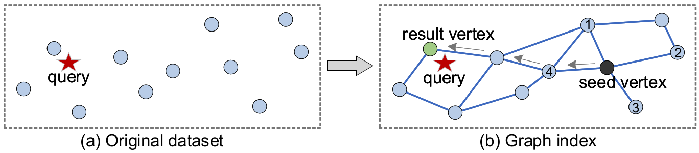
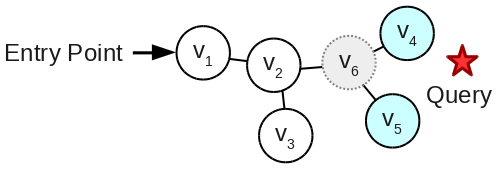
A graph-based index is constructed by overlaying a graph on top of the vectors in $\mathbb{R}^{D}$ space, so that each node $v_{i}$ is positioned over the vector $\mathbf{x}_{i}$ within the space. This induces distances over the nodes, $d(v_{i},v_{j})=d(\mathbf{x}_{i},\mathbf{x}_{j})$, which are then used to guide vector search along the edges. An example is shown in Figure 7.

The main consideration for these indexes is edge selection, in other words deciding which edges should be included during graph construction.

Graph-based indexes encapsulate all the partitioning techniques. Many graphs rely on random initialization or random sampling during construction. The $k$-nearest neighbor graph (KNNG) eppstein1997 ; paredes2005 associates each vector with its $k$ nearest neighbors through an iterative refinement process similar to $k$-means and which we consider to be a form of unsupervised learning. Other graphs, including monotonic search networks (MSNs) dearholt1988 and small-world (SW) graphs malkov2014 ; malkov2020 , aim to be highly navigable, but differ in their construction. The former tend to rely on search trials that probe the quality of the graph harwood2016 ; fu2019 ; subramanya2019 while the latter use a heuristic procedure which we refer to as “one-shot refine”. Table 5 shows several graph indexes.

Figure 7: In this example from wang2021comprehensive , a graph is overlayed on top of the original dataset (a). Search begins from a “seed” vertex and is guided along the edges until it reaches the nearest node (vector) to the query (b).

Table 5: Representative graph-based indexes.

Type	Index	Initialization	Construction
KNNG	KGraph dong2011	Random KNNG	Iterative refine
	EFANNA	Random trees	Iterative refine
MSN	FANNG harwood2016	Empty graph	Random trial
	NSG fu2019	Approx. KNNG	Fixed trial
	Vamana subramanya2019	Random graph	Fixed trial
SW	NSW malkov2014	Empty graph	One-shot refine
	HNSW malkov2020	Empty graph	One-shot refine

Graph-based search techniques have been shown to perform well in practice li2020 , and recent analytical results suggest that asymptotic performance approaches the $N^{\rho}$ and $N^{1+\rho}$ limits achieved by LSH, albeit with $\rho=c^{2}/(2c^{2}-1)$ but smaller constant factors laarhoven2018 ; prokhorenkova2020 . An experimental comparison of graph-based techniques is available in wang2021comprehensive .

3.3.1 $k$-Nearest Neighbor Graphs

In a KNNG, each node $v_{i}$ is connected to $k$ nodes representing the nearest neighbors to $\mathbf{x}_{i}$ eppstein1997 . For batched queries, $\mathbf{q}$ can be considered as a member of $S$, and a KNNG built over $S$ allows exact $k$-NN search in $O(1)$ time through a simple look-up.

A KNNG can also be used to answer interactive queries, where $\mathbf{q}\notin S$. The basic idea is to recursively select node neighbors that are nearest to $\mathbf{q}$, starting from initial nodes, and add them into the top-$k$ result set. The search complexity depends on the number of iterations before the result set converges. The search can start from multiple initial nodes, and if there are no more node neighbors to select, it can be restarted from new initial nodes wang2012query .

A KNNG can be exact or approximated with a technique which we refer to as “iterative refine”.

Exact. An exact KNNG can be constructed by performing a brute force search $N$ number of times, giving a total complexity of $O(DN^{2})$. Unfortunately, there is little hope for improvement, as it is believed that the complexity is bounded by $N^{2-o(1)}$ williams2018 . An $O(N\log N)$ algorithm is given in vaidya1989 but with a constant factor that is $O(D^{D})$. The algorithm in paredes2006 achieves an empirical complexity of $O(N^{2-\epsilon})$, where $0<\epsilon<1$. This finding suggests the existence of efficient practical algorithms, despite the worst-case bounds.

Iterative Refine. An approximate KNNG can be obtained by iteratively refining an initial graph. We give two examples.

• NN-Descent. The NN-Descent (KGraph) method dong2011 begins with a random KNNG and iteratively refines it by examining the neighbors of the neighbors of each node $v_{i}$, replacing edges to $v_{i}$ with edges to these second-order neighbors that are closer. When the dataset is growth restricted, then each iteration is expected to halve the radius around each node and its farthest neighbor. This property leads to fast convergence, with empirical times on the order of $O(N^{2-\epsilon})$ for $0<\epsilon<1$.

• EFANNA. Instead of starting from a random KNNG, EFANNA uses a forest of randomized $k$-d trees to build the initial KNNG. Doing so is shown to lead to higher recall and faster construction, as it can quickly converge to better local optima. A similar approach is taken in wang2012 but where the tree is constructed via random hyperplanes.

3.3.2 Monotonic Search Networks

A KNNG is not guaranteed to be connected. Disconnected components complicates the search procedure for online queries by requiring restarts to achieve high accuracy paredes2005 ; wang2012query . But by adding certain edges so that the graph is connected, it becomes possible to follow a single path beginning from any initial node and arriving at the nearest neighbor to $\mathbf{q}$.

A search path $v_{1}\dots v_{m}$ is monotonic if $d(v_{i},\mathbf{q})>d(v_{i+1},\mathbf{q})$ for all $i$ from $1$ to $m-1$. An MSN is a graph where the search path discovered by a “best-first” search, in which the neighbor of $v_{i}$ that is nearest to $\mathbf{q}$ is greedily selected, is always monotonic. This property implies a monotonic path for every pair of nodes in the graph and that the graph is connected.

The search complexity depends on the sum of the out-degrees over the nodes in the search path. If there are few total edges in the graph, then the search complexity is likely to be small. The minimum-edge MSN that guarantees exact NNS is believed to be the Delaunay triangulation navarro2002 . But constructing a triangulation requires at least $\Omega(N^{\lceil D/2\rceil})$ time edelsbrunner1996 , impractical for large $N$ and $D$. As a result, several approximate methods have been developed, but these necessarily sacrifice the search guarantee.

In the early work by dearholt1988 , an MSN is constructed in polynomial time by refining a sub-graph of the Delaunay triangulation called the relative neighborhood graph (RNG), introduced in toussaint1980 and later reviewed in jaromczyk1992 . The RNG itself is not monotone, but it can be constructed in $O(DN^{2-o(1)}\log^{1-o(1)}N)$ time under $\mathbb{R}^{D}$ Euclidean distance su1991 . But the $N^{2-o(1)}$ term makes this approach impractical for large $N$.

Instead of repeatedly scanning the nodes, search trials can be used to probe the quality of the graph. Depending on the path taken by best-first search, new edges are added so that a monotonic path exists between source and target. The algorithm is shown below.

procedure MakeMSN($S$)

     $G\leftarrow\text{InitializeGraph(S)}$

     repeat

         $(s,t)\leftarrow\text{ChooseSourceTargetPair}(S)$

         $P\leftarrow\text{GetSearchPath}(G,(s,t))$

         $\text{UpdateOutNeighbors}(G,t,P)$

         for each $p\in P$ do

              $\text{UpdateOutNeighbors}(G,p,t)$

         end for

     until $\text{Terminate}()$

     return $G$

end procedure

For InitializeGraph, some indexes begin with an empty graph harwood2016 , random graph subramanya2019 , or approximate KNNG fu2019 . Simple graphs can be initialized quickly but more complex graphs may offer better quality. For ChooseSourceTargetPair, one way is to select random pairs harwood2016 , while another is to designate a node as the source for all search trials subramanya2019 ; fu2019 . We refer to these techniques as random and fixed trials, respectively.

Random Trial. Indexes based on random trials are constructed over a large number of iterations, with each one leading to closer approximations of an MSN. The construction time can thus be adjusted with respect to the quality of the graph.

• FANNG. In the Fast ANN Graph harwood2016 , graph construction terminates after a fixed number of trials, e.g. $50N$. The UpdateOutNeighbors routine adds an edge between $t$ and the nearest node in the search path, $p^{*}\in P$, and then prunes out-neighbors of $p^{*}$ based on “occlusion” rules derived from the triangle inequality in order to limit out-degrees. The empirical storage and search complexities are reported to be on the order of $O(DN^{1-\epsilon})$.

Fixed Trial. In fixed trial construction, all trials are conducted from a special designated source node, sometimes called the “navigating” node. This node also serves as the source for all online queries. Normally, the index is constructed by conducting one trial to each node in a single pass over $S$. The construction complexity is generally about $O(DN^{1+\epsilon}\log N^{\epsilon})$ where the logarithmic term represents the cost of the search trials.

• Navigating Spreading-Out Graph. The NSG index fu2019 starts from an approximate KNNG. For UpdateOutNeighbors, it uses an edge selection strategy based on lune membership, similar to dearholt1988 . To guarantee that all targets are reachable from the navigating node, it overlays a spanning tree to connect any unreachable targets.

• Vamana. To speed up construction, Vamana subramanya2019 begins with a random graph instead of an approximate KNNG, and instead of checking lune membership, UpdateOutNeighbors uses a simple distance-based threshold similar to FANNG harwood2016 .

[b] Structure Index^a Partitioning Residence Complexity^b Update^c Error Bound Constr. Space Query Table E²LSH datar2004 Space Mem. Med. High Med. Y ✓ FALCONN andoni2015optimal Space Mem. Med. High Med. R ✓ *SQ Discrete Mem. Med. Low Med. Y ✗ *PQ Clustering Mem. Med. Low Med. R ✗ *IVFSQ Clustering Mem. Med. Low Med. R ✗ *IVFADC jegou2011product Clustering Mem. Med. Low Med. R ✗ SPANN chen2021 Clustering Disk Med. Med. Med. R ✗ Tree FLANN muja2009 Space Mem. High High Low R ✗ RPTree dasgupta2008 ; dasgupta2013 Space Mem. Low High Low R ✓ *ANNOY Space Mem. Low High Low R ✗ Graph NN-Descent (KGraph) dong2011 Proximity Mem. Med. Med. Med. N ✗ EFANNA Proximity Mem. High Med. Low N ✗ FANNG harwood2016 Proximity Mem. High Med. Med. N ✗ NSG fu2019 Proximity Mem. High Med. Low N ✗ Vamana (DiskANN) subramanya2019 Proximity Disk Med. Med. Low N ✗ *HNSW malkov2020 Proximity Mem. Low Med. Low Y ✗

Table 6: Representative search indexes.

• An asterisk (*) indicates supported by more than two commercial VDBMSs.

• Based on theoretical results reported by authors, empirical results reported by authors, or our own cursory analysis when no results are reported. Key for complexity columns, with $0\leq\epsilon\leq 1$ and a natural constant, $K$: – Construction. High=worse than $O(DN^{1+\epsilon})$, Med.=$O(DN^{1+\epsilon})$, Low=$O(DN\log N)$; – Size. High=$O(DN\cdot K)$ or worse, Med.=$O((D+K)\cdot N)$, Low=$O(N\log D)$; – Query. High=worse than $O(DN^{\epsilon})$, Med.=$O(DN^{\epsilon})$, Low=$O(D\log N)$.

• Y=data independent updates; R=updates with rebalancing; N=no updates.

3.3.3 Small World Graphs

Figure 8: Example HNSW index. Two nodes are randomly assigned to the top layer (orange), two to the middle layer (blue), and three to the bottom layer (purple). The out-degrees in each layer are bounded by $k$ to modulate search complexity. Vertical edges allow the search algorithm to traverse down the layers, while horizontal edges allow traversal within a layer.

A graph is small-world if the length of its characteristic path grows in $O(\log N)$ watts1998 . A navigable graph is one where the length of the search path found by the best-first search algorithm scales logarithmically with $N$ kleinberg2000 . A graph that is both navigable and small-world (NSW) thus possesses a search complexity that is likely to be logarithmic, even in the worst case.

• NSW. An NSW graph can be constructed using a procedure which we call one-shot refine and detailed in malkov2014 . Nodes are sequentially inserted into the graph, and when a node is inserted, it is connected to its $k$ nearest neighbors already in the graph.

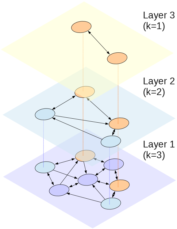
• HNSW. While NSW offers search paths that scale in $\log N$, the out-degrees also tend to scale in the logarithm of $N$, leading to polylogarithmic search complexity. In malkov2020 , a hierarchical NSW (HNSW) graph is given which uses randomization in order to restore logarithmic search. During node insertion, the node is assigned to all layers below a randomly selected maximum layer, chosen from an exponentially decaying distribution so that the size of each layer grows logarithmically from top to bottom. Within each layer, the node is connected to its neighbors following the NSW procedure, but where the out-degrees are bounded. Best-first search proceeds from the top-most layer. Figure 8 shows an example.

3.4 Discussion

As seen from Table 6, HNSW offers many appealing characteristics. It is easy to construct, has reasonable storage requirements, can be updated, and supports fast queries. It therefore comes as no surprise that it is supported by many commercial VDBMSs. The storage cost may still be a concern for very large vector collections, but there are ways to address this.

Even so, there are cases where other indexes may be more appropriate. For batched queries or workloads where the queries belong to $S$, KNNGs may be preferred, as once they are constructed, they can answer these queries in $O(1)$ time. KGraph is easy to construct, but EFANNA is more adaptable to any online queries. For online workloads, the choice rests on several factors. If error guarantees are important, then an LSH-based index or RPTree can be considered. If memory is limited, then a disk-based index such as SPANN or DiskANN may be appropriate. If the workload is write-heavy, then table-based indexes may be preferred, as they generally can be efficiently updated. Out of these, E²LSH is data independent and requires no rebalancing. For read-heavy workloads, tree or graph indexes may be preferred, as they generally offer logarithmic search complexity.

Aside from these indexes, there have also been efforts at mixing structures in order to achieve better search performance. For example, the index in azizi2023 and the Navigating Graph and Tree (NGT) index ngt use a tree to initially partition the vectors and then use a graph index over each of the leaf nodes.

4 Query Optimization and Execution

There may be multiple ways to execute a given query. The goal of the query optimizer is to select the optimal query plan, typically the latency minimizing plan.

To achieve this goal, the first step is plan enumeration, followed by plan selection and then query execution. For predicated queries, vector indexes can not be easily combined with attribute filters in the same plan, resulting in the development of new hybrid operators.

4.1 Hybrid Operators

Predicated queries can be executed by either applying the predicate filter before vector search, known as “pre-filtering”; after the search, known as “post-filtering”; or during search, known as “single-stage filtering”.

If the search is index-supported, then there needs to be a mechanism to inform the index that certain vectors are filtered out. For pre-filtering, block-first scan works by “blocking” out vectors in the index before the scan is conducted wei2020 ; wang2021 ; gollapudi2023 . The scan itself proceeds as normal but over the non-blocked vectors. For single-stage filtering, visit-first scan works by scanning the index as normal, but meanwhile checking each visited vector against the predicate conditions wu2022 .

Figure 9: Under best-first search, blocking out node $v_{6}$ makes the blue cluster of nodes, comprising the true nearest neighbor, unreachable from the entry point.

4.1.1 Block-First Scan

Blocking can be done online at the time of a query, or if predicates are known beforehand, it can be done offline.

Online Blocking. For online blocking, the aim is to perform the blocking as efficiently as possible in order to minimize the impact on query latency. In AnalyticDB-V wei2020 and Milvus milvus ; wang2021 , a technique using bitmasks is given. A bitmask is constructed using traditional attribute filtering techniques. Then, during index scan, a vector is quickly checked against the bitmask to determine whether it is “blocked”.

Offline Blocking. For graph-based indexes, blocking can cause the graph to become disconnected, as shown in Figure 9. In Filtered-DiskANN gollapudi2023 , the aim is to prevent disconnections in the first place by strategically adding edges based on the attribute category of adjoining nodes. A similar preventative approach is used in Qdrant qdrant for HNSW and in wu2022 .

In Milvus milvus ; wang2021 , $S$ is pre-partitioned along attributes that are expected to be predicate targets. When a query arrives, it can then be executed on the relevant partition using a normal index scan.

4.1.2 Visit-First Scan

For low-selectivity predicates, visit-first scan can be faster than online blocking because there is no need to block the vectors beforehand. But if the predicate is highly selective, then visit-first scan risks frequent backtracking as the scan struggles to fill the result set.

One way to avoid backtracking is to infuse the scan operator with a traversal mechanism that incorporates attribute information. In gollapudi2023 , the filter condition is added to the best-first search operator. In wu2022 , the distance function used for edge traversal is augmented with an attribute related component so that the scan favors nodes that are likely to pass the filter.

4.2 Plan Enumeration

As vector search queries tend to consist of a small number of operators, in many cases predefining the plans is not only feasible but also efficient, as it saves overhead of enumerating the plans online. But for systems that aim to support more complex queries, the plans cannot be predetermined. For extended VDBMSs based on relational systems, relational algebra can be used to express these queries, allowing automatic enumeration.

4.2.1 Predefined

For predefined plans, the main consideration is which plan to specify for which query. Some systems target specific workloads, thereby focusing on single plans per query. Other systems predefine multiple plans.

Single Plan. Single plans can be highly efficient as it removes the overhead of plan selection in addition to enumeration, but can be a disadvantage if the predefined plan is not suited to the particular workload.

A non-predicated query trivially has a single query plan when only one type of search method is available. For example in EuclidesDB euclid , each database instance is configured with one search index which is used for every search query. This can also be true for predicated queries. For example in Weaviate, all predicated search queries are executed by pre-filtering. Meanwhile in Vearch vearch ; li2018 , all predicated search queries are executed using post-filtering.

Multiple Plans. For non-predicated queries, different indexes lead to multiple plans. For example, AnalyticDB-V wei2020 supports brute force scan and table-based index scan over PQ or VGPQ. This allows a $k$-NN query to be executed using either of these methods.

Predicated queries can be answered either by pre-filtering, post-filtering, or single-stage filtering. But different vector search indexes, along with the presence or absence of an attribute index, multiply the number of possible plans.

4.2.2 Automatic

For automatic enumeration, some VDBMSs based on relational systems take advantage of the underlying relational optimizer to perform plan enumeration as well as selection. The relational language is extended to support distance functions and vector index scans. For example, pgvector pgvec and PASE yang2020 both take advantage of PostgreSQL support for user extensions.

4.3 Plan Selection

To identify the optimal query plan, existing VDBMSs perform plan selection either by using handcrafted rules or by using a cost model.

4.3.1 Rule Based

(a)

(b)

Figure 10: Plan selection rules in (a) Qdrant and (b) Vespa.

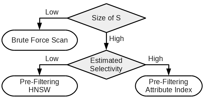
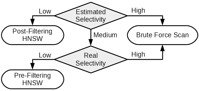
If the number of plans is small, then selection rules can be used to decide which plan to execute. Figure 10 shows two examples, used by Qdrant qdrant (Figure 10a) and Yahoo Vespa vespa (Figure 10b).

Both Qdrant and Vespa perform plan selection based on the estimated selectivity of the predicate. In Qdrant, a predicated $k$-NN query can be executed by a brute force scan, pre-filtering with an attribute index, or pre-filtering with HNSW. Plan selection is based on two thresholds, one on the size of $S$ and the other on the selectivity of the filter. If $S$ is small, then a brute force scan is performed. On the other hand, if the selectivity is high, meaning a small fraction of $S$ passes the filter, then the attribute index is used, otherwise HNSW is used. In Vespa, a predicated query can additionally be executed by using HNSW followed by post-filtering when the selectivity estimate is low. Moreover, if the estimate does not immediately favor brute force scan or post-filtering, then Vespa will apply the filter, and then choose between a brute force scan over the filtered collection or a blocked HNSW scan based on the actual selectivity. Existing methods cormode2011 are used for estimating selectivity.

4.3.2 Cost Based

Plan selection can also be performed using a cost model, choosing the plan with the least estimated cost.

In AnalyticDB-V wei2020 and Milvus milvus ; wang2021 , a linear cost model sums the component costs of the individual operators to yield the cost of each plan. The basic operator cost depends on the number of distance calculations as well as memory and disk retrievals performed by the operator. For predicated queries, these numbers are estimated from the selectivity of the predicate. But they also depend on the desired query accuracy, which is exposed to the user as an adjustable parameter. The effect of different accuracy levels on operator cost is determined offline.

We point out several unaddressed challenges to cost estimation for predicated queries. For pre-filtering with best-first search, the cost of the scan can be hard to estimate due to uncertainty around the amount of blocking. This applies more to tree or graph-based indexes, as for table-based indexes, the cost of a scan is bounded above by bucket size. Likewise for visit-first scan, the cost of the scan depends on the rate of predicate failures, which is hard to know beforehand.

On the other hand, post-filtering for a predicated $k$-NN query may lead to a result set that contains fewer than $k$ items. In VDBMSs that use post-filtering, this is often mitigated by retrieving $\alpha k$ nearest vectors instead of just the $k$ nearest. But higher $\alpha$ make search more expensive, and there is no clear way for deciding on the optimal value which minimizes search cost while guaranteeing $k$ results in the final result set.

4.4 Query Execution

Vector operators can take advantage of hardware acceleration such as via processor caches, SIMD instructions, and GPUs in order to reduce query latency. A VDBMS can also use distributed search to reduce the computing burden for a single machine, and to increase throughput, multiple searches can be conducted in parallel over the distributed cluster. For write-heavy workloads, a VDBMS can sacrifice consistency for write throughput by using out-of-place updates, which allow index updates to be deferred until more suitable times.

4.4.1 Hardware Acceleration

Vector comparison requires reading full vectors into the processor. This aspect of vectors along with large size complicates disk retrieval, but this same locality makes them amenable to hardware accelerated processing.

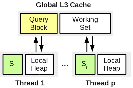
CPU Cache. If data is not present in the processor cache, then it must be retrieved from memory, stalling the processor. As shown in Figure 11, Milvus milvus ; wang2021 minimizes cache misses for batched queries by partitioning the queries into query blocks, which are small enough to fit into the CPU cache. The queries are answered a block at a time, and multiple threads can be used to process the queries. As each thread references the entire block when performing a search, the block is safe from eviction under the common eviction policies.

Figure 11: Cache friendly query blocks used by Milvus milvus ; wang2021 .

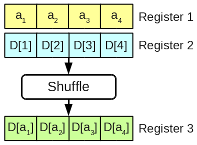
Single Instruction Multiple Data (SIMD). The original ADC algorithm performs a series of table look-ups and summations (see Example 2). While SIMD instructions can trivially parallelize the summations, look-ups require memory retrievals (in the case of cache misses) and are more difficult to speed up. But in andre2017 ; andre2021 , the SIMD shuffle instruction is cleverly exploited to parallelize these look-ups within a single SIMD processor. This technique is implemented in Faiss faiss .

The basic idea is illustrated in Figure 12. The look-up indices, plus the entire look-up table, are stored into the SIMD registers. The shuffle operator is then used to rearrange the values of the table register so that the $i$th entry contains the value at the $i$th index, lining up the values for the subsequent additions.

The table is aggressively compressed in order to fit it into a register. First, centroids are represented using 4 bits instead of a more customary 8 bits, yielding a total of $2^{4}=16$ centroids. Second, the distances in the table are quantized into 8-bit integers. The result is that there are only 16 8-bit integers in the look-up table, fitting inside a typical 128-bit register. In andre2021 , some improvements are made to allow more values to be stored in the register, namely variable-bit centroids and splitting up large tables across multiple registers.

Figure 12: Performing table look-up with SIMD.

Graphical Processing Units (GPUs). A GPU consists of a large number of processing units in addition to a large device memory. The threads within a processing unit are grouped together in “warps”, and each warp has access to a number of 32-bit registers shared across the threads. An architectural diagram can be found in lindholm2008 .

In johnson2021 , an ADC search algorithm for GPUs is given, also as a part of Faiss. Similar to the SIMD algorithm, the GPU algorithm likewise tries to avoid memory retrievals, this time from GPU device memory. It also achieves this by performing table look-ups within the registers, taking advantage of a shuffle operator called “warp shuffle”.

If the running $k$ nearest neighbors are tracked in the registers, then $k$ cannot be too large. Milvus milvus ; wang2021 works around this issue by conducting a $k$-NN over multiple rounds, flushing intermediate results store in the registers into host memory after each round.

4.4.2 Distributed Search

Many VDBMSs vald ; pine ; milvus ; wang2021 ; guo2022 ; qdrant ; vespa ; wei2020 take advantage of distributed clusters in order to scale to larger datasets or greater workloads. Some that are offered as a cloud service take advantage of disaggregated architectures in order to offer high elasticity. We point readers to wang2023disaggregated for details about these architectures.

To perform a distributed search, the vector collection is first partitioned into shards. The collection can be partitioned into equal shards, where the vectors in the shards are identically distributed, or partitioned based on other characteristics, for example based on index key for collections that are bucketed using a table-based index. A local index can then be built for each shard, and shards and their local indexes can also be replicated to provide fault tolerance and to increase throughput, as multiple queries can be executed simultaneously over the replicas.

Distributed vector search follows a scatter-gather pattern. The query is first scattered to all the relevant shards, then the result set is obtained by aggregating the results from each shard. For example for a $k$-NN query, each shard produces a result set containing the $k$ nearest neighbors to the query that are members of the shard, and then a central coordinator gathers and merges these results to produce the final result set.

4.4.3 Out-Of-Place Updates

Updating an index in-place, even for fast update structures such as HNSW, can disrupt search queries if the index cannot be used during this time. These disruptions can be severe if updates take a long time or during a lengthy rebuild.

Replicas. Some VDBMSs mitigate this issue by partitioning the vector collection into shards and replicas, and then constructing a local index over each replica vald ; weaviate ; wei2020 . In this way, if the index on one replica is undergoing an update or rebuild, queries can be handled by a different replica without any disruption. But the storage (memory) requirements are multipled by the number of replicas, and there may be extra overhead for search queries due to scatter-gather.

Log-Structured Merge (LSM) Tree. Another approach is to stream updates into a separate structure and then reconciled against the index at a more convenient time. An LSM tree oneil1996 ; luo2020 solves the problem that read-friendly indexes cannot support fast writes, and write-friendly update structures such as differential files and append-only logs cannot support fast reads.

In Milvus milvus ; wang2021 and Manu guo2022 , a vector search index is constructed over each segment of the LSM tree in order to support fast reads. A new index is created whenever a segment becomes full or is merged.

Other Techniques. In Vald vald , updates are streamed into a simple queue, and then applied in bulk to the local index once the queue is full or based on other conditions. Likewise in AnalyticDB-V wei2020 , updates are kept in memory and periodically merged with older records that are kept on disk.

5 Current Systems

[b] Name Type Sub- Type Vector Query Query Variant Vector Index Ex. Ap. Rng. Pr. Mul. Bat. Tab. Tr. Gr. Opt. EuclidesDB (2018) euclid Nat. Vec. ✓ ✓ ✗ ✗ ✗ ✗ ✓ ✓ ✓ ✗ Vearch (2018) vearch ; li2018 Nat. Vec. ✗ ✓ ✗ ✓ ✗ ✗ ✓ ✗ ✗ ✗ Pinecone (2019) pine Nat. Vec. ✗ ✓ ✗ ✓ ✓ ✗ Proprietary U Vald (2020) vald Nat. Vec. ✓ ✓ ✓ ✗ ✗ ✓ ✗ ✗ ✓ ✗ Chroma (2022) chroma Nat. Vec. ✗ ✓ ✗ ✓ ✗ ✗ ✗ ✗ ✓ U Weaviate (2019) weaviate Nat. Mix ✗ ✓ ✓ ✓ ✓ ✗ ✗ ✗ ✓ ✗ Milvus (2021) milvus ; wang2021 Nat. Mix ✓ ✓ ✓ ✓ ✓ ✓ ✓ ✗ ✓ ✓ NucliaDB (2021) nuclia Nat. Mix ✗ ✓ ✓ ✓ U ✗ ✗ ✗ ✓ ✗ Qdrant (2021) qdrant Nat. Mix ✓ ✓ ✓ ✓ ✓ ✓ ✗ ✗ ✓ ✓ Manu (2022) guo2022 Nat. Mix ✓ ✓ ✓ ✓ ✓ ✓ ✓ ✗ ✓ ✓ Marqo (2022) marqo Nat. Mix ✗ ✓ ✗ ✓ ✓ ✓ ✗ ✗ ✓ U Vespa (2020) vespa Ext. NoSQL ✓ ✓ ✓ ✓ ✓ ✗ ✗ ✗ ✓ ✓ Cosmos DB (2023) Ext. NoSQL ✗ ✓ ✗ ✗ ✗ ✗ ✓ ✗ ✗ ✗ MongoDB (2023) Ext. NoSQL ✗ ✓ ✗ ✓ ✗ ✗ ✗ ✗ ✓ ✗ Neo4j (2023) Ext. NoSQL ✗ ✓ ✗ ✗ ✗ ✗ ✗ ✗ ✓ ✗ Redis (2023) Ext. NoSQL ✓ ✓ ✓ ✓ ✗ ✓ ✗ ✗ ✓ ✗ AnalyticDB-V (2020) wei2020 Ext. Rel. ✓ ✓ ✓ ✓ ✗ ✗ ✓ ✗ ✓ ✓ PASE+PG (2020) yang2020 Ext. Rel. ✓ ✓ ✓ ✓ ✗ ✗ ✓ ✗ ✓ ✓ pgvector+PG (2021) pgvec Ext. Rel. ✓ ✓ ✓ ✓ ✓ ✗ ✓ ✗ ✓ ✓ SingleStoreDB (2022) single ; prout2022 Ext. Rel. ✓ ✗ ✓ ✓ ✗ ✗ ✗ ✗ ✗ ✓ ClickHouse (2023) click Ext. Rel. ✓ ✓ ✓ ✓ ✗ ✗ ✗ ✓ ✓ ✓ MyScale (2023) my Ext. Rel. ✓ ✓ ✓ ✓ ✗ ✗ ✓ ✗ P ✓

Table 7: A list of current VDBMSs. Dates are estimated from paper publication, earliest Github release, blog post, or other indications. Dates indicate year when vector search capability first appeared in the product.

• Abbreviations: Ex.=exact $k$-NN; Ap.=ANN; Rng.=range; Pr.=predicated; Mul.=multi-vector; Bat.=batched; Tab.=table; Tr.=tree; Gr.=graph; Opt.=query optimizer; Nat.=native; Ext.=extended; Vec.=mostly vector; Rel.=relational; U=unknown; P=proprietary.

The variety of data management techniques has led to an equally diverse landscape of commercial VDBMSs. They can be broadly categorized as native systems, which are designed specifically for vector data management, and extended systems, which add vector capabilities on top of an existing system. Table 7 lists several of these systems.

5.1 Native

Native systems are characterized by small query APIs, simple processing flows composed of a low number of components, and basic storage models, making them highly specialized at vector data management.

These systems can be further divided into two subcategories, those that target mostly vector workloads euclid ; vearch ; pine ; vald ; chroma , where the vast majority of queries access the vector collection, and those that target mostly mixed workloads weaviate ; milvus ; nuclia ; qdrant ; guo2022 ; marqo , where queries are also expected to access non-vector collections. Mostly mixed workloads may consist of traditional attribute queries or textual keyword queries, along with typical predicated and non-predicated vector queries.

5.1.1 Mostly Vector

Mostly-vector systems are designed to support fast search queries over large vector collections. Several systems, such as EuclidesDB euclid and Vald vald , focus exclusively on non-predicated queries. Others, such as Vearch vearch , Pinecone pine , and Chroma chroma offer predicated queries but supported by a single predefined plan. These systems often support only a single search index, typically graph-based. Hence, they have no need for a query parser, rewriter, or optimizer, and can omit these components in order to reduce processing overhead. They also typically do not support exact search, as all queries are handled by the index.

Figure 13: EuclidesDB euclid supports multiple vector spaces so that query results can be more semantically accurate.

We point out some examples.

• EuclidesDB. EuclidesDB euclid , shown in Figure 13, is a system for managing embedding models, aimed at allowing users to experiment over various models and similarity scores in order to find the most semantically meaningful setting. Users bring their own embedding models and interact with the system by querying and manipulating non-vector entities.

• Vald. Vald vald is a serverless VDBMS aimed at providing scalable non-predicated vector search. Instead of a single centralized system, Vald spans a Kubernetes cluster consisting of multiple “agents”. The vector collection is sharded and replicated across the agents to increase throughput and decrease latency via scatter-gather. An individual Vald agent contains an NGT graph index built over its local shard. Vald also supports out-of-place updates on each local replica using a simple update queue.

• Vearch. Vearch vearch ; li2018 is targeted at image-based search for e-commerce, allowing it to be designed specifically toward this aim. Predicated queries are supported, but they are all executed using post-filtering, considered to be sufficient for the application. Vearch also has no need to support exact queries. Vearch adopts a disaggregated architecture with dedicated search nodes, allowing it to scale read and write capabilities independently.

Pinecone pine offers a scalable distributed system similar to Vald, but as it is offered as a managed cloud-based service, it can be a more user-friendly option. Chroma chroma is a centralized system similar to EuclidesDB, meant for a single machine.

5.1.2 Mostly Mixed

Mostly-mixed systems aim to support more sophisticated queries compared to mostly-vector systems. In general, they support a greater variety of basic queries, including more support for exact and range queries, in addition to more query variants. These systems likewise have no need for query rewriters or parsers, but some, such as Milvus milvus ; wang2021 , Qdrant qdrant , and Manu guo2022 , make use of query optimization. Other systems, including Weaviate weaviate , NucliaDB nuclia , and Marqo marqo , also have more sophisticated data and storage models in order to deal with predicated queries and attribute-only queries that go beyond simple retrieval.

• Milvus and Manu. Milvus milvus ; wang2021 is aimed at comprehensive support for vector search queries, and Manu guo2022 adds additional features on top of Milvus. All three basic query types are supported, in addition to the three query variants. Multiple search indexes are also supported, and predicated queries are handled by a cost-based optimizer.

• Qdrant. Qdrant qdrant likewise supports a large variety of search queries. For predicated queries, it uses a rule-based optimizer coupled with a custom HNSW index designed for block-first scan.

• NucliaDB and Marqo. NucliaDB nuclia and Marqo marqo are targeted at document search and retrieval and use vector search to provide semantic retrieval. A key feature is the support for combining keywords and vectors through multi-vector search. Non-vector keyword queries are processed using text specific techniques, resulting in sparse term-frequency vectors. These vectors are then combined with dense feature vectors through an aggregate score in order to conduct multi-vector search.

• Weaviate. Weaviate targets document search and retrieval over a graph model. This allows Weaviate to answer non-vector queries, such as retrieving all books written by a certain author, in addition to similarity queries via vector search. Users interact with Weaviate by issuing queries written in GraphQL.

5.2 Extended

Extended systems inherit all the capabilities of an underlying data management system and are necessarily more complex compared to native systems. But these systems are also more capable. Nearly all the extended systems listed in Table 7 support all three basic query types and multiple indexes, and all of them support query optimization. These systems likewise divide into two subcategories, those where the underlying system is NoSQL and those where it is relational.

5.2.1 NoSQL

Many of the hallmarks of a NoSQL system davoudian2018 , such as schemaless storage, distributed architecture, and eventual consistency, are present in native systems, making a NoSQL extended VDBMS much like a native system.

• Vespa. Vespa vespa is a scalable distributed NoSQL system designed for large scale data processing workloads. Unlike native systems, Vespa aims at more general data processing tasks, hence it is equipped with a flexible SQL-like query language. But like native systems, the storage model is simple, provided by an in-house document store. Vespa uses a rule-based query optimizer.

• Cassandra. Cassandra lakshman2010 is a popular distributed NoSQL system based on a wide column store. Vector search capability will be available in version 5.0 by integrating HNSW into the storage layer, implementing scatter-gather across replicas, and extending the Cassandra query language with vector search operators.

• Databricks. The Spark-based Databricks platform is expected to support vector search, including predicated queries, in an upcoming version.

Aside from Vespa, several other document based NoSQL databases have now been extended to support vector search, including MongoDB, Cosmos DB, and Redis, when coupled with the Redis Stack search extension. Vector search capability has also been extended to NoSQL systems other than document stores. For example, Neo4j is a property graph database with experimental vector search capability. So far, only ANN queries are supported, using HNSW.

5.2.2 Relational

For extended relational systems, their features mostly come from the inherent capabilities of relational systems. For example, SQL already is sufficient for expressing $(c,k)$-search queries, and these queries can already be answered by most relational engines upon adding a user-defined similarity function. This is perhaps exemplified by SingleStore single ; prout2022 , which offers exact $k$-NN and range search through its native relational engine, without any vector search indexes. Subsequently, extended relational systems focus more on tightly integrating vector search capability alongside existing components.

• SingleStore. SingleStore single ; prout2022 is a cloud-native hybrid transactional and analytical (HTAP) database li2022 based on a distributed row store for fast writes alongside column store replicas for fast reads. Vector search is handled by the native relational engine, extended with functions for calculating dot product and Euclidean distance.

• PASE. PASE yang2020 extends PostgreSQL with a flat quantization index and HNSW index in order to support vector search.

• pgvector. The pgvector pgvec extension for PostgreSQL brings a vector data type, functions over this data type, and flat and HNSW index access methods into PostgreSQL. Vector queries are issued using SQL. If an index is created over a vector column, then queries are answered using the index, yielding approximate results. Otherwise, exact brute force scan is used. Plan selection is performed by the existing PostgreSQL query optimizer using the generic cost estimator, or by calling index-specific cost estimators to refine the estimate, if needed. Other features such as replication, fault tolerance, access controls, concurrency control, and so on, are provided by PostgreSQL.

• AnalyticDB-V. AnalyticDB-V wei2020 adds vector search capability on top of AnalyticDB zhan2019 . This is achieved primarily by introducing vector indexes, VGPQ and HNSW, and by augmenting the cost-based optimizer.

• ClickHouse and MyScale. ClickHouse click is a columnar database aimed at fast analytics coupled with an asynchronous merge mechanism for fast ingestion. It supports vector queries using ANNOY and HNSW. Likewise, MyScale my is a cloud service using ClickHouse as the backend. It adds table-based search indexes including flat indexes and IVFADC, and a proprietary search index called “multi-scale tree graph” (MSTG) which is shown to outperform both IVFADC and HNSW.

5.3 Libraries and Other Systems

Vector search engines and libraries make up a third category in the broader ecosystem. Typically, these are embedded into applications that require vector search, but they lack the capabilities of a full VDBMS.

Search Engines. Apache Lucene lucene is a pluggable search engine that provides sophisticated search capability for embedded applications. Latest versions offer vector search, supported by HNSW. While Lucene itself lacks higher level features such as multi-tenancy, distributed search, and administrative features, many of these are provided by search platforms built on top of Lucene, including Elasticsearch elastic , OpenSearch open , and Solr solr . These capabilities could make Lucene an attractive alternative to mostly-vector native VDBMSs as it offers similar features and can readily integrate with existing infrastructure.

Libraries. There are also libraries that directly implement specific indexes. For example, KGraph is an implementation of the NN-Descent KNNG. The Microsoft Space Partition Tree and Graph (SPTAG) library sptag combines several techniques, including SPANN and NGT, into one configurable index. Libraries are also available for LSH, including E2LSH and FALCONN. Likewise, Meta Faiss faiss offers a selection of indexes, including HNSW, an LSH family for Hamming distance, and quantization-based indexes.

Other Systems. Other systems are aimed at other parts of the broader pipeline. Featureform is a middleware aimed at dataset management. Similar to relational ETL tools, it offers a means of organizing the workflows that transform raw data sources into curated datasets to be consumed by downstream applications. Featureform exposes some of these downstream functions through its API. For example, it offers a vector search endpoint that executes a $k$-NN query over a configured provider, such as Pinecone. On the other hand, Activeloop Deep Lake hambardzumyan2023 offers tensor operations directly over a tensor warehouse, making it capable of performing vector search inside the warehouse.

Aside from vector search, vector visualization can also be a useful tool for data analysts. Nomic Atlas offers a platform for visualizing high-dimensional vector spaces by projecting them onto two-dimensional plots using a proprietary dimensionality reduction technique.

5.4 Discussion

The designs of these databases cover a spectrum of characteristics involving query processing and vector storage, manifesting in a range of performance and capabilities, as shown in Figure 14.

We offer a few broad remarks. Native mostly-vector systems broadly offer high performance but are targeted at specific workloads, sometimes even specific queries, and thus have relatively limited capability. Meanwhile, native mostly-mixed systems offer more capabilities, notably predicated queries, and some such as Milvus milvus ; wang2021 , Qdrant qdrant , and Manu guo2022 also perform query optimization. These, along with extended NoSQL systems, achieve a comfortable balance between high performance and search capabilities. On the other hand, extended relational systems offer the most capabilities but possibly less performance. But, as has been mentioned elsewhere, relational systems are already major components of industrial data infrastructures, and being able to conduct vector search without introducing new systems into the infrastructure is a compelling advantage. The ranking shown in Figure 14 is consistent with empirical observations aumuller2020 .

Thus, we imagine that future work will target systems that can offer both high performance in addition to offering unified data management capabilities, represented by the arrow in Figure 14.

Figure 14: High-level characteristics of VDBMSs.

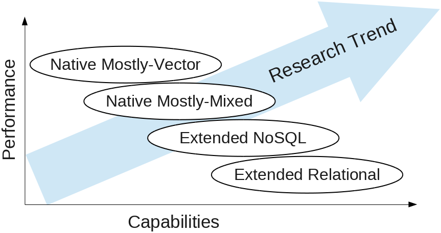
6 Benchmarks

Comprehensive cross-disciplinary comparisons of vector search algorithms and systems are surprisingly scarce, attributed to the wide range of fields from which search algorithms arise li2020 . We point out two notable attempts at benchmarking these algorithms and systems.

In li2020 , a large number of ANN algorithms are uniformally implemented and evaluated across a range of experimental conditions. These algorithms include LSH, L2H, methods based on quantization, tree-based techniques, and graph-based techniques. The experiments are conducted over 18 datasets, ranging from a few thousand vectors to 10 million vectors, and with dimensions ranging from 100 to 4,096. The feature vectors are derived from real-world image, text, video, and audio collections, as well as synthetically generated. Algorithms are measured on query latency as well as the quality of the result sets based on precision, recall, and two other derivative measures.

In aumuller2020 , the evaluation is extended to include full VDBMSs in addition to isolated algorithms. Whereas li2020 aims to avoid the effects of different implementations, here these differences are kept in order to more accurately reflect real-world conditions. The standardized evaluation platform and the latest benchmark results are available online, with results for several VDBMSs. The datasets, however, are smaller in both size and dimensionality than the ones used in li2020 .

7 Challenges and Open Problems

While much progress has been made on vector data management, some challenges remain unaddressed.

Similarity Score Selection. The semantic quality of different similarity scores is still challenging to understand, and there is no rigorous guidance on how to select which score for which scenarios. Systems like EuclidesDB euclid can be used to experimentally determine the best scores and embedding models, but outside of wang2023 , this problem remains unexplored.

Operator Design. Designing efficient and effective hybrid operators remains challenging. For graph indexes, block-first scan can lead to disconnected components that either need to be repaired or that require new search algorithms for handling this situation. Existing offline blocking techniques gollapudi2023 ; milvus ; wang2021 ; qdrant are limited to small number of attribute categories. For visit-first scan, estimating the cost of the scan is challenging due to unpredictable backtracking, complicating plan selection.

Incremental Search. Some applications, such as e-commerce and recommender platforms, make use of incremental $k$-NN search, where $k$ is effectively very large but is retrieved in small increments so that the results appear to be seamlessly delivered to the user. While techniques exist for this type of search fisher2012 , it is unclear how to support this search inside vector indexes.

Multi-Vector Search. Multi-vector search is also important for certain applications such as face recognition. Existing techniques tend to use aggregate scores, but this can be inefficient as it multiplies the amount of distance calculations. Generic multi-attribute top-$k$ techniques also are hard to adapt to vector indexes wang2021 , and there are no works on MQMF queries.

Security and Privacy. As vector search becomes increasingly mission-critical, data security and user privacy become more important, especially for VDBMSs that offer managed cloud services. There is thus a need for new techniques that can support private and secure high-dimensional vector search xue2018 .

8 Conclusion

In this paper, we surveyed vector database management systems aimed at fast and accurate vector search, developed in response to recent popularity of dense retrieval for applications such as LLMs and e-commerce. We reviewed considerations for query processing, including similarity scores, query types, and basic operators. We also reviewed the design, search, and maintenance considerations regarding vector search indexes. We described several techniques for query optimization and execution, including plan enumeration, plan selection, operators for predicated or “hybrid” queries, and hardware acceleration. Finally, we discussed several commercial systems and the main benchmarks for supporting experimental comparisons.