SwG-former: Sliding-window Graph Convolutional Network Integrated with Conformer for Sound Event Localization and Detection

Abstract

Sound event localization and detection (SELD) is a joint task of sound event detection (SED) and direction of arrival (DoA) estimation. SED mainly relies on temporal dependencies to distinguish different sound classes, while DoA estimation depends on spatial correlations to estimate source directions. To jointly optimize two subtasks, the SELD system should extract spatial correlations and model temporal dependencies simultaneously. However, numerous models mainly extract spatial correlations and model temporal dependencies separately. In this paper, the interdependence of spatial-temporal information in audio signals is exploited for simultaneous extraction to enhance the model performance. In response, a novel graph representation leveraging graph convolutional network (GCN) in non-Euclidean space is developed to extract spatial-temporal information concurrently. A sliding-window graph (SwG) module is designed based on the graph representation. It exploits sliding-windows with different sizes to learn temporal context information at different levels of granularity and dynamically constructs graph vertices in the frequency-channel (F-C) domain to capture higher abstraction levels for spatial correlations. Furthermore, as the cornerstone of message passing, a robust Conv2dAgg function is proposed and embedded into the SwG module to aggregate the features of neighbor vertices. In order to improve the performance of SELD in a natural spatial acoustic environment, a general and efficient SwG-former model is proposed by integrating the SwG module with the Conformer. It exhibits superior performance in comparison to recent advanced SELD models. To further validate the generality and efficiency of the SwG-former, it is seamlessly integrated into the event-independent network version 2 (EINV2) called SwG-EINV2. The SwG-EINV2 surpasses the state-of-the-art (SOTA) methods under the same acoustic environment.

Keywords Sound event localization and detection  $\cdot$ Graph convolution network  $\cdot$ Graph aggregation function  $\cdot$ Conformer

1 Introduction

In the presence of overlapping auditory signals, the human ear has an innate ability to effortlessly localize each sound source and discern the sound of interest. How can machines have a similar capability to localize and distinguish overlapping sounds? Sound event localization and detection (SELD) aims to tackle this challenge and has extensive applications such as monitoring systems [1, 2, 3, 4], smart homes [5, 6, 7], security systems [8], wildlife protection [9, 10], virtual reality [11], and intelligent conference rooms [12, 13, 14]. SELD is designed to identify the classes, onset, and offset of sound events from multi-channel audio signals and estimate the spatial localizations of the corresponding sound events, which integrates the subtasks of sound event detection (SED) and direction of arrival (DoA) estimation.

SED mainly relies on temporal dependencies to distinguish different sound classes, while DoA estimation depends on spatial correlations recorded amplitude and phase differences between microphones to estimate source directions. The input features for SELD consist of multi-channel log-mel spectrograms concatenated along with the intensive vectors (IVs), where spatial information is encoded in the frequency-channel (F-C) information. To jointly optimize two subtasks, the SELD system should extract F-C information to capture spatial correlations and model temporal dependencies simultaneously.

Significant progress for SELD has been achieved following a series of challenges, including the detection and classification of acoustic scenes and events (DCASE) challenge [15] and the IEEE ICASSP grand challenge-L3DAS [16]. Emerging models can be primarily classified into multi-branch and single-branch output formats.

Adavanne et al. [15] proposed the SELDNet, which is implemented by a convolutional recurrent neural network (CRNN) and outputs two branches to predict SED and DoA separately. Cao et al. [17] proposed the event-independent network version 2 (EINV2), which is based on the soft-parameter sharing mechanism of convolutional neural network (CNN) blocks and multi-head self-attention (MHSA) [18]. The EINV2 further adopts a track-wise output format for detecting overlapping sound events of the same class but with different DoAs. Hu et al. [19] improved EINV2 by incorporating Conformer [20] and dense blocks. However, the model is parameter-heavy due to the integration of different models.

Shimada et al. [21] regarded SELD as a Cartesian regression task, merging SED and DoA representations into a single-branch output, called active coupling cartesian direction of arrival (ACCDOA). This method overcomes the loss balance issue in dual-branch output. Later, Shimada et al. [22] introduced a multi-ACCDOA format that handles overlapping instances from the same class while maintaining a class-wise output format. Consequently, multi-ACCDOA became a prevalent output format. Wu et al. [23] enhanced the original CRNN by inserting a shallow multilayer perceptron-mixer (MLP-Mixer) between the convolution filters and the recurrent layers to model inter-channel audio patterns intricately. Wang et al. [24] introduced a model that combines CRNN, MHSA technique, and a CNN-Transformer encoder to explore various model structures incorporating attention mechanisms. Wang et al. [25, 26] used a ResNet-Conformer structure as the backbone network, where ResNet is used to extract spatial features, and Conformer is adopted to mode temporal context dependencies. Shul et al. [27] proposed the divided spectro-temporal attention model to construct sequential contextual relationships in the frequency and temporal domains separately.

Most of these methods employ CNN to extract spatial information and gate recurrent unit (GRU) to extract temporal features separately. In this paper, however, the interdependence of spatial-temporal information in audio signals is exploited for simultaneous extraction to enhance the model performance, as experimentally discussed in section 4.4.

Inspired by the convolution 3D (C3D) network [28] simultaneously extracting spatial-temporal information from videos, a novel graph representation that leverages graph convolutional network (GCN) in non-Euclidean space is proposed to simultaneously extract spatial-temporal information of audio, as detailed in Fig. 1. The graph representation converts audio signals into graph signals with non-Euclidean structure. It is analogous to considering height and width as a spatial domain in the videos that the graph representation treats the F-C domain as a unified domain in multi-channel audios. Further, the sliding-window graph (SwG) module, dividing the audio feature into time chunks with different sizes, exploits sliding-windows to learn temporal context information at different levels of granularity. Meanwhile, it dynamically constructs graph vertices based on the similarities between vertices in the F-C domain to capture spatial correlations. As the cornerstone of message passing, a more robust convolution 2D aggregation (Conv2dAgg) function is embedded into the SwG module to aggregate the features of neighbor vertices. Further, a general and efficient SwG-former model is proposed by integrating the SwG module with the Conformer. SwG-former captures higher abstraction levels for spatial-temporal information by the SwG module and models global context interactions by the MHSA module. Experimental results show better performance for the SwG-former than recent advanced SELD models. To substantiate the generality and efficiency of SwG-former, SwG-former has been seamlessly integrated into the EINV2 framework [19], achieving a state-of-the-art (SOTA) performance.

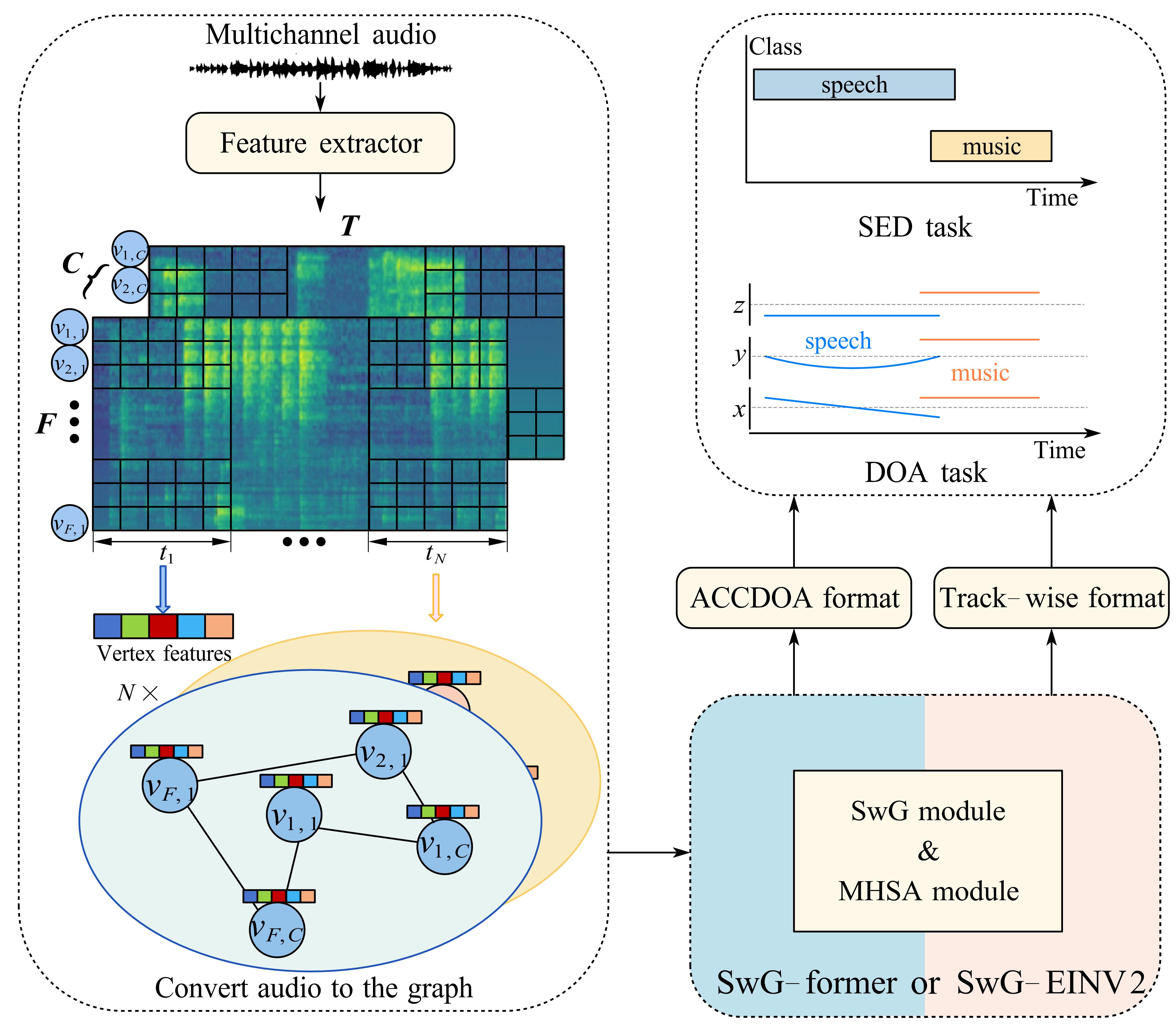
Figure 1: The sketch of the SELD system. The feature extractor first obtains the feature with the dimension of $T\times F\times C$, and $T$ is divided into $N$ time chunks evenly. $T,F$, and $C$ represent time frame, frequency bin, and channel, respectively. A graph is dynamically constructed in the frequency-channel domain within each chunk. In a total of $F\times C$ vertices $V=\{{{v}_{i,j}}|i=1,...,F,j=1,...C\}$, $T/N$ time frames are served as the features of these vertices. These constructed graphs are then fed to the SwG-former or SwG-EINV2, designed to extract spatial features and model context dependencies simultaneously. The SED and DoA final results are outputted in the ACCDOA [22] or track-wise [17] format.

The main contributions of the paper can be summarized as follows:

1. A universal and novel method is proposed to convert audio signals into graph data structures, efficiently extracting spatial-temporal features concurrently. It is the first study that employs GCN for SELD task.

2. The SwG module is proposed to learn temporal context information at different levels of granularity. It employs sliding-windows to divide the audio features into different-sized time chunks and dynamically constructs graph vertices in the F-C domain to capture spatial correlations.

3. A more robust Conv2dAgg function is proposed to implement stronger fitting capabilities than the standard graph aggregation function. It adopts 2D convolutional kernels to aggregate the features of neighbor vertices efficiently.

4. The plug-and-play SwG-former is designed for the SELD task. It displays superior results compared with other methods by embedding the SwG module in Conformer. Further, it integrated with the EINV2 framework surpasses the SOTA methods.

The remainder of the paper is organized as follows: Section 2 introduces the theoretical background of GCN. Section 3 describes the architectures of SwG-former and SwG-EINV2 models, the designed SwG module, and the proposed Conv2dAgg function. The dataset, experimental setup, and a series of ablation studies aimed at exploring superior model performance, along with the experimental results and a visualization analysis, are presented in Section 4. Finally, the conclusion is given in Section 5.

2 Related work

2.1 Graph convolutional networks

To overcome the challenge posed by the inability of CNN to process non-Euclidean data, graph neural networks (GNNs) emerged. Early GNNs [29] were primarily applied to address strict graph theory problems on graphs $\mathsf{\mathcal{G}}=(V,\mathsf{\mathcal{E}})$. The $\mathsf{\mathcal{G}}$ is composed of vertices set $V$ and edges set $\mathsf{\mathcal{E}}$. The GNNs were usually applied to social networks [30], traffic forecasting [31, 32], chemical molecular structure prediction [33, 34], recommendation engines [32, 35], and so on. It was not until Bruna et al. [36] first proposed the spectral GCN and spatial GCN that their application in audio-related tasks became prosperous. Shirian et al. [37] proposed compact graph convolutional networks for speech emotion recognition tasks. Tzirakis et al. [38] treated audio channels as vertices to construct graph structures and adopted GCN to extract the spatial correlation among different channels for multi-channel speech enhancement. Wang et al. [39] encoded more structural details based on GCN for speech separation.

The implementation of GCN on audio-related tasks is mainly based on the spectral GCN, which decomposes the graph Laplacian matrix to aggregate neighbor vertex features. However, the operation of eigenvalue decomposition will bring unbearable costs once the graph structures become more complex. Based on this, the spatial GCN method aggregates information from neighbor vertices and avoids the eigenvalue decomposition. Hence, the spatial GCN is applied in the SELD task.

2.2 Aggregation functions of spatial GCNs

The aggregation function is proposed for spatial GCN to aggregate the vertex features from neighbor vertices. It can be mainly divided into parameter-less max [40, 41, 42], mean [43]functions, and parameterized functions like long short-term memory (LSTM). Hamilton et al. [41] empirically found that max and LSTM outperform mean aggregation. Veličković et al. [44]proposed graph attention networks (GATs) that learn the attention weights between the central vertex and the neighbor vertices through an attention mechanism [45]. Furthermore, Xu et al. [46] proposed graph isomorphism networks (GIN) that adopt sum aggregation, which demonstrates discriminative power equivalent to the Weisfeiler-Lehman graph isomorphism test [47]. Additionally, Li et al. [48] adopted max-relative (MR) graph convolution to aggregate neighbor vertex features through max pooling operation without learnable parameters. These aggregation functions can handle variable-length data but at the expense of some fitting ability, which means each neighbor vertex aggregated by the same weight $w$, defined as:

$${{\operatorname{Agg}}_{1}}\left({{\mathbf{h}}_{i}}\right)=\sum\limits_{{{\mathbf{h}}_{j}}\in\mathsf{\mathcal{N}}\left({{\mathbf{h}}_{i}}\right)}{w{{\mathbf{h}}_{j}}},$$ (1)

where ${{\mathbf{h}}_{j}}\in\mathsf{\mathcal{N}}({{\mathbf{h}}_{i}})$ is the feature of the vertex ${{v}_{i}}$ and ${{\mathbf{h}}_{j}}\in\mathsf{\mathcal{N}}({{\mathbf{h}}_{i}})$ $j\in 1,...,k$ is neighbor vertex features of ${{v}_{i}}$. In contrast, the CNN aggregation function is denoted as:

$${{\operatorname{Agg}}_{2}}\left({{\mathbf{h}}_{i}}\right)=\sum\limits_{{{\mathbf{h}}_{j}}\in\mathsf{\mathcal{N}}\left({{\mathbf{h}}_{i}}\right)}{{{w}_{j}}{{\mathbf{h}}_{j}}},$$ (2)

where there are $k$ weights ${{w}_{i}}$ ($j\in 1,...,k$) for the convolutional kernel. As a result, CNN has stronger fitting capabilities than GCN but at the expense of handling variable-length data. In the proposed GCN aggregation function, information from these neighbor vertices can be aggregated by Eq. (2) because each vertex is associated with a fixed number of neighbor vertices.

3 Proposed framework

3.1 Network architectures

This section describes the SwG-former, a simple and plug-and-play model. It processes SED and DoA tasks within a single branch and outputs in the ACCDOA format. To have an extensive comparison with complex models that output in the track-wise format, the SwG-former blocks take the place of the Conformer blocks within the EINV2 framework, named SwG-EINV2. The seamless integration of SwG-former substantiates its generality.

3.1.1 SwG-former model

SwG-former model first processes the input with 4 layers of multi-scale convolution (MS-Conv) blocks and 5 layers of SwG-former blocks. MS-Conv block utilizes trainable weights to fuse multi-scale features to extract high-level spatial features, as illustrated in Fig. 5. SwG-former block extracts spatial-temporal information concurrently. The data flow is sustained at 250 frames to capture abundant sequence information and then condensed to 50 frames through max pooling operation. Subsequently, the fully connected (FC) layers with the tanh function map the output of SELD onto a unit circle in the ACCDOA format. Further details are illustrated in Fig. 2.

The SwG-former block retains a pair of macaron-like Feed Forward (FF) modules, sandwiching other modules from the Conformer block. It replaces the convolution module with the SwG module, which captures higher abstraction levels for spatial information compared with the convolution module. It learns the spatial correlations inherent in dynamic sound scenes by dynamically changing graph structures at different layers. If the SwG module uses an oversized sliding-window to extract global temporal information, it will impose a computational burden. To alleviate this, the MHSA module assists in modeling global context dependencies in the speech sequence.

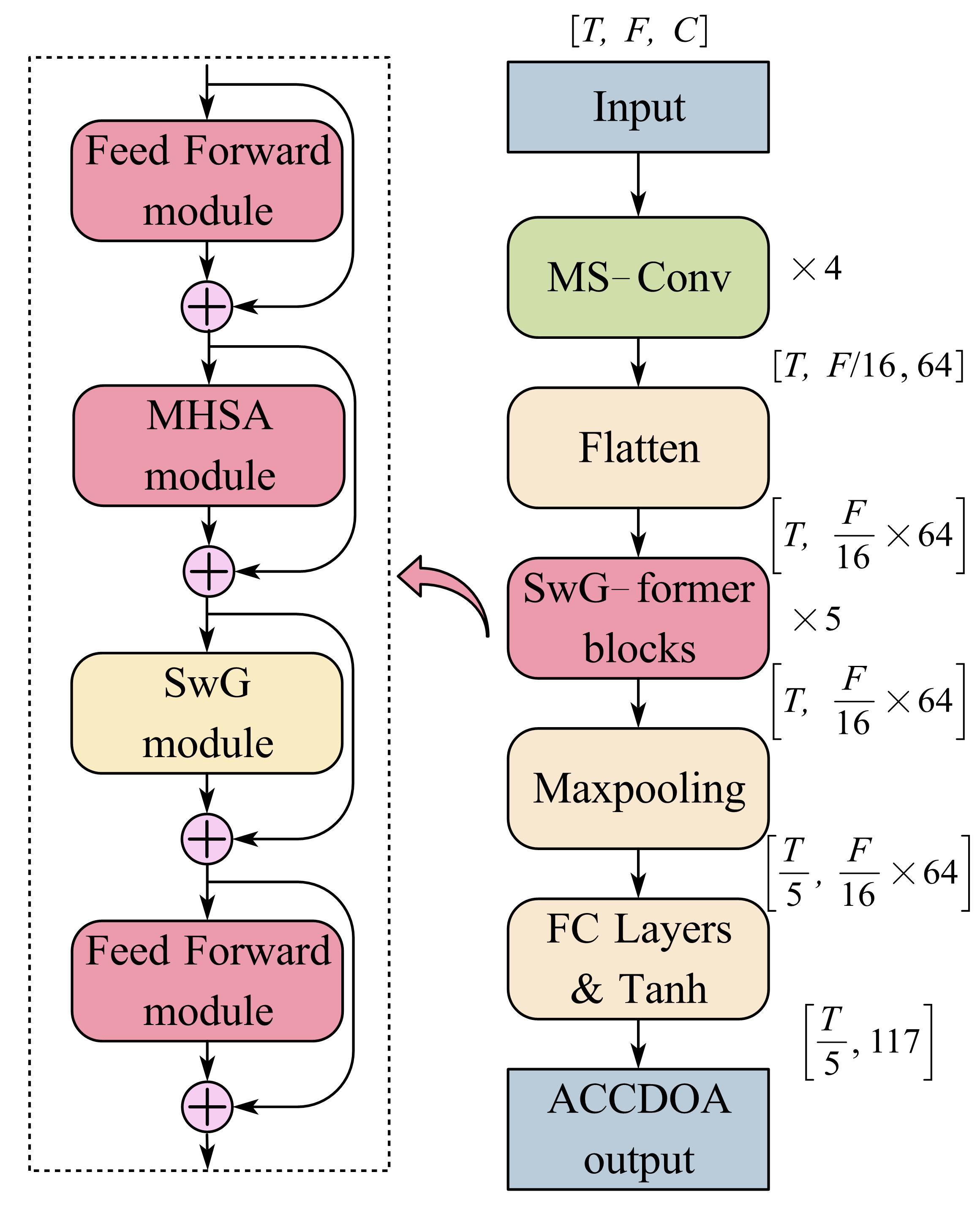
Figure 2: The architecture of SwG-former model.

3.1.2 SwG-EINV2 model

SwG-EINV2 model employs SwG-former blocks to replace the Conformer ones within the EINV2 framework [17, 18]. The pink blocks signify the SED task, whereas the blue blocks represent the DoA estimation task. Four-channel log-mel spectrograms are input into the SED branch, while the DoA branch receives both 4-channel log-mel spectrograms and 3-channel IVs. Four layers of Dual Conv, as shown in Fig. 5, process the input and then condense time frames to reduce the model parameters. The green boxes denote the soft parameter-sharing between the SED and DoA subtasks, meaning different subtasks utilize their respective feature layers instead of the same ones. Finally, SwG-EINV2 employs the track-wise output format to manage up to 3 overlapping sound events, as illustrated in Fig. 3.

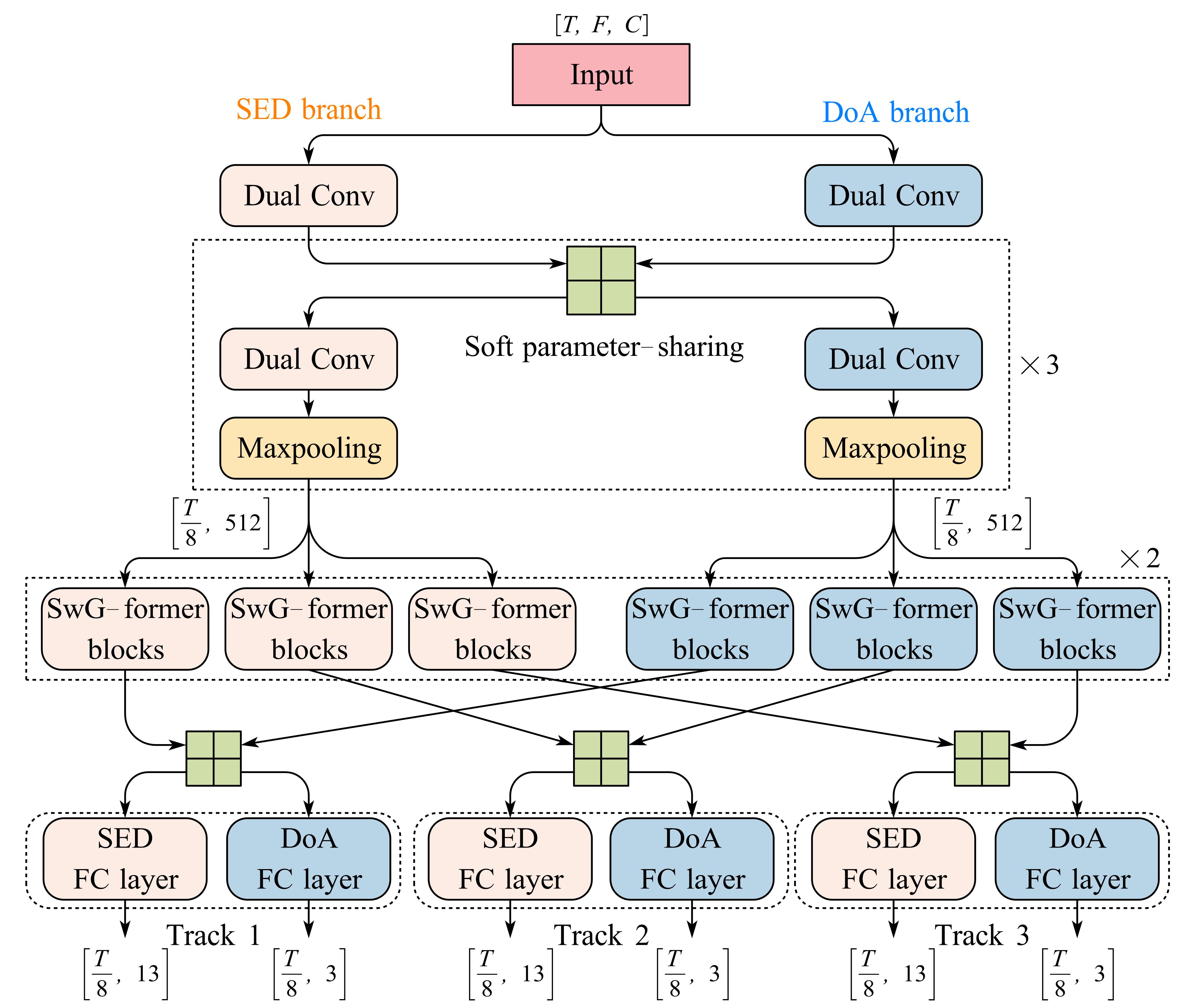
Figure 3: The architecture of SwG-EINV2 model.

3.2 Sliding-window graph module

The SwG-former and SwG-EINV2 models both have the SwG module as a cornerstone of transforming the audio signal into a graph representation, illustrated in Figs. 2 and 3. Additionally, Fig. 4 provides a schematic representation of how the SwG module learns temporal context information at different levels of granularity and extracts F-C features to capture spatial correlations. Notably, the SwG module processes audio data within a graph structure, offering enhanced flexibility compared with conventional spectrogram representation. Concurrently, to facilitate integration with other advanced non-graph modules, the SwG module outputs features in the spectrogram representation format.

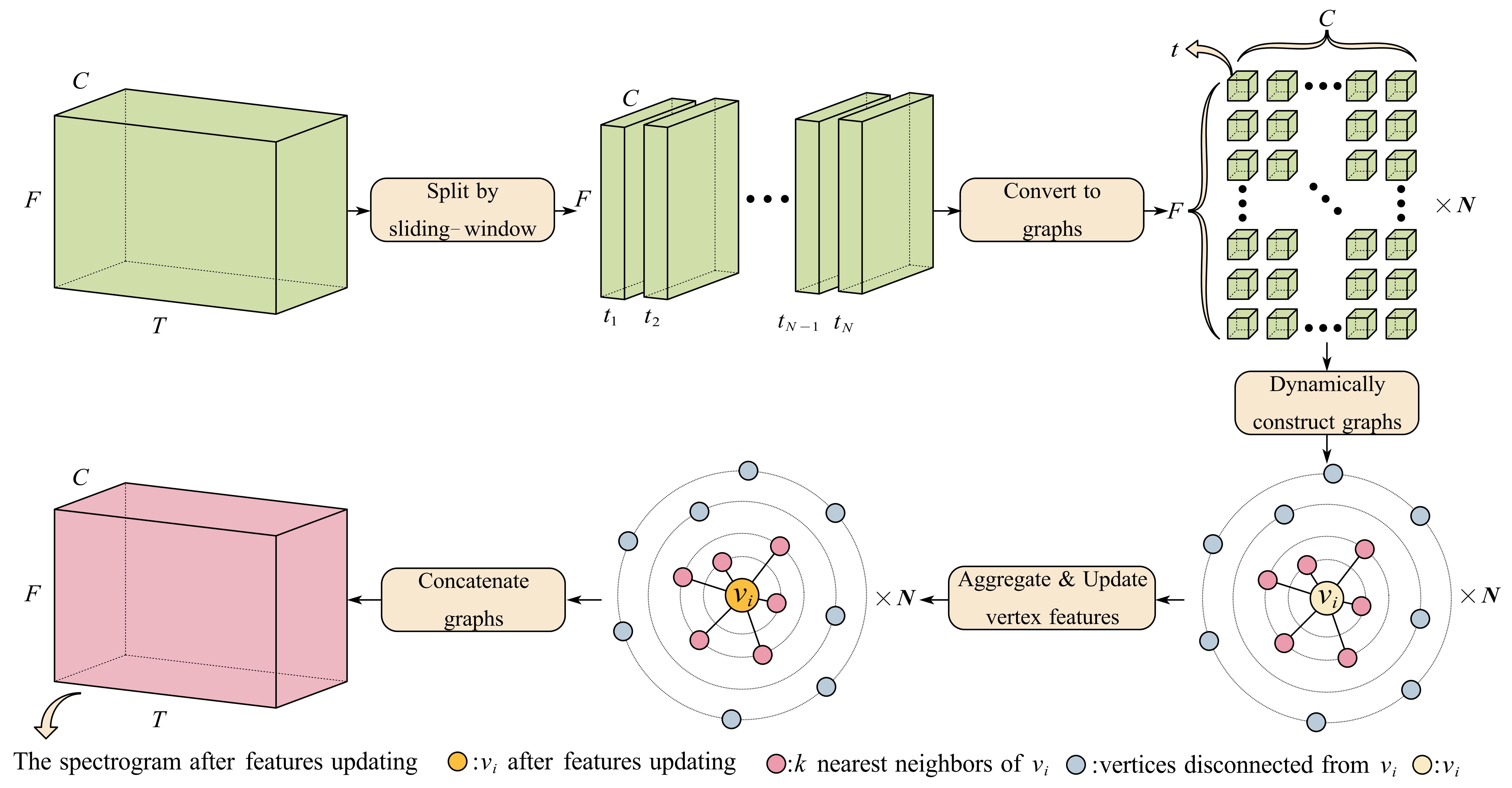
Figure 4: Flowchart of the SwG module. Vertex $v_{i}$ constructs connections with its $k$ nearest neighbors during the dynamic graph construction process. Then, $v_{i}$ aggregates and updates features from its neighbor vertices. Subsequently, the generated $N$ graphs are concatenated along the time axis into a spectrogram structure for subsequent processing by other modules.

3.2.1 Input features

The first-order Ambisonics (FOA) format 4-channel audio dataset is employed. The feature extractor in Fig. 1 first extracts 4-channel log-mel spectrograms and 3-channel IVs. The log-mel spectrograms, with IVs concatenated along with channel dimension, are fed into MS-Conv blocks illustrated in Fig. 5 to extract high-level spatial features as the input features of the SwG module.

Figure 5: Multi-scale convolution (MS-Conv) block.

The proposed MS-Conv block utilizes two dual convolution layers with $3\times 3$ and $5\times 5$ kernels to extract multi-scale features. The multi-scale features are then fused with residual connection using trainable weights ${{w}_{1}}$,${{w}_{2}}$, and ${{w}_{3}}$. The MS-Conv block is formulated as follows:

$$\mathbf{x}^{\prime}=\operatorname{Dropout}\left(\operatorname{Maxpooling}\left({{w}_{1}}{{\mathbf{x}}_{\mathbf{-}}}\mathbf{3}+{{w}_{2}}{{\mathbf{x}}_{\mathbf{-}}}\mathbf{5}+{{w}_{3}}\mathbf{x}\right)\right)$$ (3)

where $\mathbf{x}$ and $\mathbf{x}^{\prime}$ are the input and output of the MS-Conv block, respectively, ${{\mathbf{x}}_{\mathbf{-}}}\mathbf{3}$ and ${{\mathbf{x}}_{\mathbf{-}}}\mathbf{5}$ are the outputs of two dual convolutions with $3\times 3$ and $5\times 5$ kernels. The Swish activation function [49] is employed between the dual convolution layers to enhance model accuracy and convergence speed.

3.2.2 Proposed graph representation of audio signals

Let $\mathsf{\mathcal{G}}=(V,\mathsf{\mathcal{E}})$ denote a graph where $V$ and ${\mathcal{E}}$ denote the vertices and edges. The input feature $\mathbf{x}^{\prime}\in{{\mathbb{R}}^{T\times F\times C}}$ is split into non-overlapping equal chunks using a sliding-window along with the time dimension, where the sliding-window size is $t$ and $t=T/N$. Each chunk with the size of $t\times F\times C$ is denoted as a graph and each graph possesses the vertices $V=\left\{v_{1},...,v_{n}\right\}$ where $n=F\times C$. Then the feature vectors of vertices are denoted as $\mathbf{H}=\left[\mathbf{h}_{1},...,\mathbf{h}_{\mathbf{n}}\right]$where ${{\mathbf{h}}_{i}}\in{{\mathbb{R}}^{t}}$. According to the similarity of each pair of vertices, each vertex ${{v}_{i}}$ finds its $k$ nearest neighbors. The time chunks are fed into the SwG module to extract latent spatial-temporal features. In the shallower layers, $t$ is set as 5 to extract local temporal features. In the deeper layers, $t$ is set as 25 to obtain global temporal features.

The proposed graph representation for audio signals shows several compelling advantages. Primarily, the graph offers a generalized data structure, where the sequence of an audio signal can be interpreted as a particular case of a graph. With its non-Euclidean structure, this graph structure extends more flexibility than the spectrogram representation. It allows for the simultaneous extraction of latent spatial-temporal features based on the sliding-windows to learn temporal context information at different levels of granularity. Furthermore, by dynamically constructing graph vertices within the F-C domain, the graph representation learns the spatial correlations inherent in dynamic sound scenes. Furthermore, the proposed graph representation can be effectively leveraged to tackle various audio-related tasks.

3.2.3 Dynamic graph convolution network

Most GCNs come with a predefined topological structure, where vertex features are updated in each layer with a fixed graph structure. That could not better adapt to the characteristics of different data. This paper uses dynamic graph convolution to extract feature information better. The dynamic GCN constructs a weight matrix of edge sets dynamically in each layer by calculating the similarity of each pair of vertex features in the current feature space. Each vertex constructs connections by the k-nearest neighbors (KNN) algorithm to aggregate and update vertex information.

For the overall graph, the dynamic graph convolution network can be formulated as follows:

$$\mathbf{{G}^{\prime}}=\operatorname{Update}\left(\mathbf{G},\operatorname{Aggregate}\left(\mathbf{G},{{\mathbf{W}}_{\operatorname{agg}}}\right),{{\mathbf{W}}_{\operatorname{update}}}\right),$$ (4)

where $\mathbf{G}$ and $\mathbf{{G}^{\prime}}$ are the input and output of the dynamic graph convolution network, ${{\mathbf{W}}_{\operatorname{agg}}}$ and ${{\mathbf{W}}_{\operatorname{update}}}$, as the core of GCN, are the learnable weights of the $\operatorname{Aggregate}\left(\cdot\right)$ and $\operatorname{Update}\left(\cdot\right)$ operations, respectively.

For each vertex, the $\operatorname{Aggregate}\left(\cdot\right)$ operation corresponds to the aggregation function, denoted as $\operatorname{g}\left(\cdot\right)$. This function calculates the vertex representation by aggregating the features of neighboring vertices. The $\operatorname{Update}\left(\cdot\right)$ operation corresponds to the update function, symbolized as $\operatorname{f}\left(\cdot\right)$. This function is employed to compute the new vertex representation derived from the aggregated information. Equation (4) can be expressed as as follows:

$${{\mathbf{{h}^{\prime}}}_{i}}=\operatorname{f}\left({{\mathbf{h}}_{i}},\operatorname{g}\left({{\mathbf{h}}_{i}},\mathsf{\mathcal{N}}\left({{\mathbf{h}}_{i}}\right),{{\mathbf{W}}_{\operatorname{agg}}}\right),{{\mathbf{W}}_{\operatorname{update}}}\right),$$ (5)

where $\mathsf{\mathcal{N}}\left({{\mathbf{h}}_{i}}\right)$ is neighbor vertex features of ${{v}_{i}}$.

In the proposed graph structure, each vertex is associated with a fixed number of $k$ neighbor vertices instead of variable-length graph data. As a result, information from these neighbor vertices can be aggregated using $1\times k$ convolutional kernels (Eq. (2)). The proposed convolution 2D aggregation (Conv2dAgg) and feature update functions are defined as follows:

$$\operatorname{g}\left(\cdot\right)=\operatorname{Conv}\left({{\mathbf{h}}_{j}}|{{\mathbf{h}}_{j}}\in\mathsf{\mathcal{N}}\left({{\mathbf{h}}_{i}}\right)\right),$$ (6)

$$\operatorname{f}\left(\cdot\right)=\operatorname{MLP}\left({{\mathbf{h}}_{i}},\operatorname{g}\left({{\mathbf{h}}_{i}}\right),{{\mathbf{W}}_{\operatorname{update}}}\right),$$ (7)

where Conv in aggregation function is 2D convolution, the vertex feature updater f is a multilayer perceptron (MLP) with the batch normalization and Gaussian error linear unit (GeLU) [50] as the activation function.

In order to facilitate the interaction of temporal features of each vertex, the transform model is employed behind the dynamic graph convolution network (Eq. (4)) and denoted as:

$$\mathbf{Y}=\operatorname{GeLU}\left(\mathbf{{G}^{\prime}}{{\mathbf{W}}_{1}}\right){{\mathbf{W}}_{2}}+\mathbf{{G}^{\prime}}$$ (8)

where $\mathbf{Y}$ is the output of the transform model and also the input of the following dynamic graph convolution network layer, ${{\mathbf{W}}_{1}}$ and ${{\mathbf{W}}_{2}}$ are the weights of the FC layers. The FC layers increase the diversity of vertex features and alleviate the over-smoothing problem in deep GCN [51].

4 Experiments

4.1 Dataset

The DCASE 2021 and prior challenges emulate spatial and acoustic properties of soundscapes under realistic conditions. However, the synthetic dataset overlooks the natural temporal occurrences or co-occurrences of sounds within a real scene and the spatial constraints and connections inherent to such scenes. The Sony-TAu Realistic Soundscapes 2022 (STARSS22) dataset [52] is captured on natural sound scenes. This real dataset presents significant challenges in real-world acoustic environments, such as interference, overlapping sources, moving sources, and reverberation. Within these real recordings, which range from 30 seconds to 6 minutes, it is common to encounter multiple overlapping sound events with up to 5 overlapping sources. The labels are annotated both temporally and spatially. Both STARSS23 and STARSS22 represent real recordings within identical acoustic environments. However, STARSS22 offers a more significant number of advanced models conducive to comparative analysis.

This study utilizes the STARSS22 dataset as the training base for the proposed models. To address the challenges posed by the scarcity of real data, the study further augments the training data by incorporating 1200 one-minute audio samples from the synthetic dataset [53].

4.2 Evaluation metrics

The evaluation of SELD adopts the joint evaluation method [54]. The first two metrics for SED are the error rate ($ER$) and F-score (${{F}_{20{}^{\circ}}}$), which are location-dependent, that is to say, considering true positive ($TP$) only under a distance threshold $\text{T}{}^{\circ}$ from the prediction to the reference. The threshold $\text{T}{}^{\circ}$ is $20{}^{\circ}$default. The ${{F}_{20{}^{\circ}}}$ is a measure of retrieval effectiveness. $ER$ and ${{F}_{20{}^{\circ}}}$ are formulated as follows:

$$ER=\frac{D+I+S}{N},F_{20^{\circ}}=\frac{2PR}{P+R},$$ (9)

$$P=\frac{TP}{TP+FP},\text{ }R=\frac{TP}{TP+FN},$$ (10)

where $TP,FP$, and $FN$ denote the true positive, false positive, and false negative, respectively. $D,I$, and $S$ represent the deletion, insertion, and substitution errors, respectively. $P$ and $R$ are the precision and recall metrics, and $N$ is the number of reference sound events, respectively.

For DOA, the localization error ($LE$) and localization recall ($LR_{CD}$) are class-dependent, computed only across each class rather than all outputs. $LE$ is the mean angular localization error between predicted DOAs and their closest reference DOAs. $LR_{CD}$ is a recall metric without any spatial threshold and represents how successfully the system detects localization. For each class $c\in\left[1,...,C\right]$ in a time frame, the distance matrix $\mathbf{D}_{c}$ is obtained by computing the distance between references and predictions. Considering that multiple instances with the same class label exist simultaneously in the scene, the Hungarian algorithm $\mathrm{H}\left(\cdot\right)$ [55] associates the responding predictions and references. Thus, a binary association matrix $\mathbf{A}_{c}^{\left(l\right)}=\mathrm{H}\left(\mathbf{D}_{c}^{\left(l\right)}\right)$ and $l$ represents the time frame. For each class $c$, the $LE_{c}^{\left(l\right)}$ and $L{{R}_{c}}$ are formulated as:

$$LE_{c}^{\left(l\right)}=\frac{||\mathbf{A}_{c}^{(l)}\odot\mathbf{D}_{c}^{\left(l\right)}|{{|}_{1}}}{||\mathbf{A}_{c}^{(l)}|{{|}_{1}}}$$ (11)

$$L{{R}_{c}}=\frac{\sum\nolimits_{l}{||\mathbf{A}_{c}^{(l)}|{{|}_{1}}}}{\sum\nolimits_{l}{N_{c}^{(l)}}}$$ (12)

where $\odot$ denotes element-wise product, $||\cdot|{{|}_{1}}$ is L1-norm. The dimension of $\mathbf{D}_{c}^{\left(l\right)}$ is $M_{c}^{(l)}\times N_{c}^{(l)}$ where $M_{c}^{(l)}$ and $N_{c}^{(l)}$ represent the numbers of $c$-th predicted and reference events in the l time frame, respectively.

The overall $LE$ and $LR_{CD}$ could be formulated as follows:

$$LE=\frac{1}{CL}\sum\limits_{c}{\sum\limits_{l}{LE_{c}^{\left(l\right)}}}$$ (13)

$$L{{R}_{CD}}=\frac{1}{C}\sum\limits_{c}{L{{R}_{c}}}$$ (14)

The SELD score is adopted to aggregate all four metrics and formulated as follows:

$$SEL{{D}_{score}}=\frac{ER+\left(1-{{F}_{20{}^{\circ}}}\right)+\frac{LE}{180}+\left(1-L{{R}_{CD}}\right)}{4}$$ (15)

4.3 Experimental setup

The FOA format dataset is utilized in this study, and 7-channel log-mel with IV features are employed as frame-wise features extracted from the original audio data with a sample rate of 24 kHz. Further details can be found in Table 1. To simplify the representation of the sizes of sliding-windows across different layers, they are designated in Table 2.

The experimental investigations utilize the Ubuntu 20.04 operating system, with 32.00 GB of RAM, an AMD R7950X CPU, and an NVIDIA GeForce RTX 4090 GPU. All models are implemented using the Pytorch framework.

Table 1: Training hyper-parameters settings.

Models	SwG-former	SwG-EINV2
Epochs	100
Batch size	32
Pool size	(1, 2)
Dropout rate	0.05
k	24
Aggregation	Conv2dAgg
Optimizer	Adam	Adamw
Learning rate	0.0001	0.0003
Windows size	group B	group H
Layers of GCN	5	2

Table 2: The representation of different-sized sliding-windows.

[5, 25, 25, 25, 25]	[5, 5, 25, 25, 25]	[5, 5, 5, 25, 25]	[25, 25, 25, 5, 5]
group A	group B	group C	group D
[1, 1, 1, 1, 1]	[5, 5, 5, 5, 5]	[25, 25, 25, 25, 25]	[5, 5]
group E	group F	group G	group H

4.4 Separate vs. Simultaneous extraction of spatial-temporal information

This section discusses the earlier concept of simultaneously extracting spatial-temporal information for enhanced model performance, which is the impetus for integrating GCN into the SELD task. The superior performance of C3D over convolution 2D in video understanding is attributed to the capacity of C3D to capture spatial-temporal information concurrently. These experiments change the size of sliding-windows to the range of input feature frames processed by the SwG module in each layer. When the sliding-window size in each network layer is set as one, that setting of group E, the SwG module ceases to model context dependence on temporal information. It exclusively extracts spatial features in the F-C domain.

In contrast, the SwG module, with the settings of groups F, G, and B, simultaneously extracts spatial-temporal information. Groups F and G design the sliding-window sizes in each network layer as 5 and 25, respectively. This design highlights a comprehensive utilization of small and large windows for extracting local and global temporal information, respectively. Group B represents a compromised choice that balances groups F and G.

Table 3 shows the best performance of group B across the multiple experiments, demonstrating a superior SELD score of 0.416. Notably, the simultaneous groups generally outperform the separate group regarding error rate, F-score, and localization error but slightly underperform in localization recall. This can be primarily attributed to the SED task focusing more on the temporal information of audio signals. The simultaneous groups with larger windows can extract sequence context dependencies. Conversely, the DoA task places a higher emphasis on the spatial information inherent in audio signals. As such, with its ability to capture more granular spatial features, the separate group yields a marginal enhancement in localization recall. However, the overall performance of group G is somewhat inferior to that of the separate group. Group G employs large windows in every layer, which struggles to capture more granular temporal information. For instance, large windows may simultaneously process multiple classes of sound events, failing to detect and locate instantaneous sound events accurately. Groups B and F alleviate this drawback through smaller window sizes, with Group B achieving a more comprehensive performance through a reasonable window size.

Table 3: The performance of separate and simultaneous extraction in SwG-former.

	$\mathrm{ER}\downarrow$	$\mathrm{{F}_{20{}^{\circ}}}\uparrow$	$\mathrm{LE}\downarrow$	$\mathrm{LR}_{\mathrm{CD}}\uparrow$	$\mathrm{SELD}_{\mathrm{score}}\downarrow$
Group E (separate)	0.67	41.8	26.0	66.1	0.432
Group B (simultaneous)	0.64	45.2	24.5	65.7	0.416
Group F (simultaneous)	0.65	43.7	23.9	64.6	0.425
Group G (simultaneous)	0.70	41.5	23.5	64.1	0.440

To understand how group B significantly outperforms group E, Fig. 6 presents their average learning curves, evaluated across four metrics. Group B demonstrates a more rapid convergence than group E across all metrics and exhibits more minor fluctuations in its learning curves. As shown in Figs. 6 (a), (b), (e), and (f), group B consistently maintains a lower error rate and localization error. Its minimum values significantly outperform those of group E. Regarding F-score and localization recall, group B exhibits superior convergence speed and stability within the initial 20 epochs. That can be attributable to the large window size extracting temporal features. As illustrated in Figs. 6 (c), (d), (g), and (h), the F-score of group B, both overall and at its peak, significantly surpasses that of group E. At the same time, the performance of localization recall is relatively comparable between the two groups. This suggests that the simultaneous groups with a reasonable choice of window size could outperform the separate group in SwG-former.

Figure 6: Learning curves of separate and simultaneous extraction in SwG-former model.

4.5 Ablation studies

A series of ablation studies are undertaken to investigate SwG-former performance in this section. The connection strategies of modules initially determine the overall framework of the models. Subsequently, the granularity of feature processing is defined by the size of the sliding windows. Finally, the capacity of message passing among vertices is enhanced by adjusting the aggregation functions and the number of neighbors.

4.5.1 Different connection strategies

A series of ablation studies within the Conformer have substantiated the exemplary performance exhibited by a pair of FF modules surrounding the block in a macaron-style [20]. The experiments progressively explored the performance of different module connection orders in the SwG-former structure. Table 4 demonstrates that the structure with a pair of FF modules sandwiching the MHSA and SwG modules exhibits the best SELD score performance. By comparing the results from the [FF, MHSA, SwG, FF] structure, the [FF, MHSA, SwG, FF] leads to significantly better results in decreasing SELD scores from 0.484 to 0.416. The result is consistent with Conformer studies wherein macaron-style FF modules are used.

Table 4: The performance of different strategies in SwG-former. [FF, MHSA, SwG, FF] denotes SwG-former architecture that is sequentially composed of FF module, MHSA module, SwG module, and another layer of FF module.

	$\mathrm{ER}\downarrow$	$\mathrm{{F}_{20{}^{\circ}}}\uparrow$	$\mathrm{LE}\downarrow$	$\mathrm{LR}_{\mathrm{CD}}\uparrow$	$\mathrm{SELD}_{\mathrm{score}}\downarrow$
[FF, MHSA, SwG, FF]	0.64	45.2	24.5	65.7	0.416
[FF, SwG, MHSA, FF]	0.73	37.6	25.7	68.4	0.453
[FF, MHSA, FF, SwG]	0.67	39.5	25.6	64.5	0.443
[MHSA, FF, SwG, FF]	0.76	34.9	28.1	63.3	0.484

4.5.2 The size of sliding-windows

The size of the sliding-windows significantly impacts the granularity of feature processing. A window size that is too small brings more iterative processing, thereby imposing a substantial computational burden. Conversely, a window size is too large to extract local features from instantaneous sound events. Given that the input features comprise 250 frames, window sizes of 5 and 25 were ultimately selected.

Various sizes of sliding-windows were tested in the SwG-former model. Group B demonstrates the best performance in Table 5. Comparing the results from group B and group D suggests that using smaller windows followed by larger windows leads to outperformance.

Table 5: The performance of different size of sliding-windows in SwG-former.

	$\mathrm{ER}\downarrow$	$\mathrm{{F}_{20{}^{\circ}}}\uparrow$	$\mathrm{LE}\downarrow$	$\mathrm{LR}_{\mathrm{CD}}\uparrow$	$\mathrm{SELD}_{\mathrm{score}}\downarrow$
Group A	0.69	41.1	25.0	65.8	0.439
Group B	0.67	42.9	24.0	66.7	0.427
Group C	0.69	40.4	25.1	63.1	0.449
Group D	0.71	39.4	25.6	65.1	0.451

4.5.3 Type of aggregation functions

The experiments aimed to evaluate the performance of different aggregation functions, such as MR [48], SAGE [44], GIN [46], and the proposed Conv2dAgg. Table 6 illustrates the superior performance of the proposed Conv2dAgg, particularly in terms of $ER$ and ${{F}_{20{}^{\circ}}}$, where it significantly outperforms other aggregation functions. Moreover, Conv2dAgg achieves the second-best performance in terms of $LE$ and $LR_{CD}$. From the SELD score result, it is clear that the Conv2dAgg has a robust fitting capability.

Table 6: The performance of different aggregation functions in SwG-former.

	$\mathrm{ER}\downarrow$	$\mathrm{{F}_{20{}^{\circ}}}\uparrow$	$\mathrm{LE}\downarrow$	$\mathrm{LR}_{\mathrm{CD}}\uparrow$	$\mathrm{SELD}_{\mathrm{score}}\downarrow$
Conv2dAgg	0.64	45.2	24.5	65.7	0.416
MR [48]	0.67	42.9	24.0	66.7	0.427
SAGE [44]	0.70	40.5	25.6	63.2	0.450
GIN [46]	0.70	39.4	25.2	65.1	0.448

4.5.4 The Number of Neighbors

In the process of dynamically constructing the graph, the number of neighbors $k$ for each vertex determines the range of aggregated features, similar to the kernel size in CNN. A sufficient number of neighbors hinders message passing, while an excessive number of neighbors may lead to an over-smoothing problem. The results in Table 7 demonstrate that the SwG-former model performs best when the number of neighbors, $k$, is set to 24.

Table 7: The performance of different neighbors $k$ in SwG-former.

k	$\mathrm{ER}\downarrow$	$\mathrm{{F}_{20{}^{\circ}}}\uparrow$	$\mathrm{LE}\downarrow$	$\mathrm{LR}_{\mathrm{CD}}\uparrow$	$\mathrm{SELD}_{\mathrm{score}}\downarrow$
18	0.68	40.2	25.6	66.2	0.440
21	0.72	40.1	25.5	65.3	0.451
23	0.69	39.1	25.6	64.9	0.449
24	0.64	45.2	24.5	65.7	0.416
25	0.68	40.3	27.0	66.5	0.440
27	0.68	41.6	24.6	63.8	0.442
30	0.71	40.7	25.0	68.0	0.440

4.6 Comparisons with state-of-the-art methods

The first 5 rows of Table 8 illustrate that the proposed SwG-former model significantly outperforms CRNN [22], E-CRNN [23], CNN-MHSA [24] and ResNet-Conformer [25] across $ER$, ${{F}_{20{}^{\circ}}}$ and $LR_{CD}$ metrics. Specifically, the SwG-former model markedly improves upon the baseline model by 17.0 and 11.2 in terms of ${{F}_{20{}^{\circ}}}$ and $LR_{CD}$. Regarding model parameters, SwG-former models possess smaller parameter sizes than the CNN-MHSA model. Despite this, it exhibits a superior comprehensive performance SELD score of 0.416.

Table 8: Comparison of the proposed models with recent SELD models.

Models	$\mathrm{ER}\downarrow$	$\mathrm{{F}_{20{}^{\circ}}}\uparrow$	$\mathrm{LE}\downarrow$	$\mathrm{LR}_{\mathrm{CD}}\uparrow$	$\mathrm{SELD}_{\mathrm{score}}\downarrow$	Parameters
CRNN (baseline) [22]	0.71	28.2	31.6	55.3	0.513	0.4M
E-CRNN [23]	0.69	17.9	28.5	44.5	0.538	10.0M
CNN-MHSA [24]	0.67	27.0	24.4	60.3	0.483	672.0M
ResNet Conformer [25]	0.71	34.7	26.5	59.3	0.479	13.1M
SwG-former	0.64	45.2	24.5	65.7	0.416	110.8M
Conv-Conformer [19]	0.65	48.4	21.5	70.4	0.396	325.4M
SwG-EINV2	0.63	48.9	20.9	71.8	0.385	288.5M

To validate the generality and efficiency of the SwG-former, it has been seamlessly integrated with the EINV2 framework, named SwG-EINV2. Conv-Conformer [19] achieved SOTA performance based on EINV2. The final two rows of Table 8 demonstrate that the four metrics - $ER$, ${{F}_{20{}^{\circ}}}$, $LE$, and $LR_{CD}$ - uniformly outperform the Conv-Conformer, with the SELD score reaching 0.385 on the FOA format dataset without data augmentation. Within the EINV2 framework, the structure of the SwG-former is consistent with the results derived from the ablation studies. SwG-EINV2 only employs 2 layers of SwG-former blocks, reducing the model parameters compared to Conv-Conformer. Notably, the SwG-former did not undergo fine-tuning within the EINV2 framework, further underscoring its plug-and-play capability.

Figure 7: The comparison of the class-wise performance between baseline and SwG-former models.

The class-wise results are illustrated in Fig. 7. The substantial enhancements are discernible in classes such as Telephone, Walk, Door, Water tap, and Knock. In the baseline model, low values in ${{F}_{20{}^{\circ}}}$, coupled with high $LE$ for Door and Knock, pose significant challenges for the overall metrics. However, in the SwG-former model, each class has a noticeable elevation in the ${{F}_{20{}^{\circ}}}$ and $LE$. Specifically, the $LE$ for Door and Knock has seen a dramatic reduction from 180.00° to 12.04° and 12.88°, while the ${{F}_{20{}^{\circ}}}$ for Telephone has experienced a significant surge from 0.012 to 0.149. These enhancements across all classes collectively contribute to a superior overall performance.

4.7 Visualization results

To more intuitively validate the efficacy of the proposed SwG-former model in practical applications, this study randomly selected several sound event classes with different motion states from the STARSS22 dataset and visually analyzed their sound snippets. The results of this analysis are presented in Figs. 8 and 9, all of which originate from the same audio file. Given the relatively broad annotations of the STARSS22 dataset, a specific class label may correspond to multiple different instances. The visible results are divided according to sound event classes. To achieve coordinate normalization, the model mapped the output of SELD to the unit circle using the tanh function.

Figure 8 illustrates the visible results for the instantaneous sound event class "Female speech" (Class 0). Sound events of Class 0 occur around 570 and 1250 frames. It can be observed from Fig. 8 (a) that the CRNN model failed to detect the activity of this sound event accurately. However, the comparison results in Figs. 8 (a) and (c) demonstrate the effectiveness and superiority of the proposed model.

Figure 8: The visualization results for the "Female speech" (Class 0) sound snippets. The abscissa represents the number of frames in the selected audio snippet, and the ordinate corresponds to the corresponding SELD output. The red, green, and blue lines in the figure represent the x, y, and z axes in the Cartesian coordinate system, respectively.

Figure 9 shows the visualization results for the long-duration dynamic sound source "Walk" (Class 6). In the audio, Class 6 appears continuously from 0 to 500 frames, and the sound source location rushes; meanwhile, instantaneous sound sources also appear near 1300 and 1500 frames. It was observed that compared with the CRNN model, the proposed model could more consistently and robustly detect the timing and motion trajectory of the event occurrence under both long-duration and instantaneous states.

Figure 9: The visualization results for the "Walk" (Class 6) sound snippets. The abscissa represents the number of frames in the selected audio snippet, and the ordinate corresponds to the corresponding SELD output. The red, green, and blue lines in the figure represent the x, y, and z axes in the Cartesian coordinate system, respectively.

5 Conclusions and future work

The paper primarily focuses on broadening the application of GCN in SELD tasks. A novel and universal graph representation is proposed to convert audio signals into graph signals, which processes audio more flexibly compared to the conventional spectrogram representation. Based on the graph representation, the SwG module is designed by exploiting sliding-windows to learn temporal context information and dynamically constructing graph vertices in the F-C domain to capture spatial correlations. As the cornerstone of message passing, a robust 2D convolution aggregation function is proposed and embedded into the SwG module called Conv2dAgg. This function aggregates the features of neighbor vertices and enhances the fitting capability of the model. Specifically, the plug-and-play SwG-former model is proposed for the SELD task, demonstrating a robust capability to model local and global context dependencies and extract spatial correlations concurrently. Results from the comparative analysis of simultaneous or separate extraction of spatial-temporal information suggest that the simultaneous extraction with a reasonable choice of window size could outperform the separate extraction in SwG-former. Extensive ablation studies reveal that the proposed SwG-former model significantly outperforms other models on the STARSS22 dataset. To compare with complex models, the SwG-former blocks are integrated with the EINV2 framework, named SwG-EINV2. It achieves an SELD score of 0.385 even in the absence of data augmentation technologies and surpasses the SOTA methods under the same acoustic environment.

In future work, the SwG-former will be applied to the SELD audiovisual system, which takes both audio and video inputs. By utilizing the proposed graph representation, the SwG-former will effectively fuse audio and video features into a unified space, thereby facilitating the fusion of cross-modal features. This advanced feature representation approach is expected to enhance the performance of SELD significantly.

Declaration of competing interest.

The authors declare that they have no known competing financial interests or personal relationships that could have appeared to influence the work reported in this paper.

Acknowledgements.

The authors would like to thank the editor and anonymous reviewers for their valuable comments. This work was supported by National Natural Science Foundation of China (61571279).

References

- [1] Marco Crocco, Marco Cristani, Andrea Trucco, and Vittorio Murino. Audio surveillance: A systematic review. ACM Computing Surveys (CSUR), 48(4):1–46, 2016.
- [2] CJ Grobler, Carel P Kruger, Bruno J Silva, and Gerhard P Hancke. Sound based localization and identification in industrial environments. In IECON 2017-43rd Annual Conference of the IEEE Industrial Electronics Society, pages 6119–6124. IEEE, 2017.
- [3] Peter W Wessels, Jeroen v Sande, and Frits Van der Eerden. Detection and localization of impulsive sound events for environmental noise assessment. The Journal of the Acoustical Society of America, 141(5):3886–3886, 2017.
- [4] Pasquale Foggia, Nicolai Petkov, Alessia Saggese, Nicola Strisciuglio, and Mario Vento. Audio surveillance of roads: A system for detecting anomalous sounds. IEEE transactions on intelligent transportation systems, 17(1):279–288, 2015.
- [5] Mingxue Yang, Lujie Peng, Li Liu, Yujiang Wang, Zhenyuan Zhang, Zhengxi Yuan, and Jun Zhou. Lcsed: A low complexity cnn based sed model for iot devices. Neurocomputing, 485:155–165, 2022.
- [6] Weipeng He, Petr Motlicek, and Jean-Marc Odobez. Deep neural networks for multiple speaker detection and localization. In 2018 IEEE International Conference on Robotics and Automation (ICRA), pages 74–79. IEEE, 2018.
- [7] Ryu Takeda and Kazunori Komatani. Sound source localization based on deep neural networks with directional activate function exploiting phase information. In 2016 IEEE international conference on acoustics, speech and signal processing (ICASSP), pages 405–409. IEEE, 2016.
- [8] Giuseppe Valenzise, Luigi Gerosa, Marco Tagliasacchi, Fabio Antonacci, and Augusto Sarti. Scream and gunshot detection and localization for audio-surveillance systems. In 2007 IEEE Conference on Advanced Video and Signal Based Surveillance, pages 21–26. IEEE, 2007.
- [9] Selina Chu, Shrikanth Narayanan, and C-C Jay Kuo. Environmental sound recognition with time–frequency audio features. IEEE Transactions on Audio, Speech, and Language Processing, 17(6):1142–1158, 2009.
- [10] Tiago A Marques, Len Thomas, Stephen W Martin, David K Mellinger, Jessica A Ward, David J Moretti, Danielle Harris, and Peter L Tyack. Estimating animal population density using passive acoustics. Biological reviews, 88(2):287–309, 2013.
- [11] Jens Blauert and Spatial Hearing. The psychophysics of human sound localization. In Spatial hearing. MIT Press Cambridge, MA, USA, 1997.
- [12] Carlos Busso, Sergi Hernanz, Chi-Wei Chu, Soon-il Kwon, Sung Lee, Panayiotis G Georgiou, Isaac Cohen, and Shrikanth Narayanan. Smart room: Participant and speaker localization and identification. In Proceedings.(ICASSP’05). IEEE International Conference on Acoustics, Speech, and Signal Processing, 2005., volume 2, pages ii–1117. IEEE, 2005.
- [13] Pawel Swietojanski, Arnab Ghoshal, and Steve Renals. Convolutional neural networks for distant speech recognition. IEEE Signal Processing Letters, 21(9):1120–1124, 2014.
- [14] Taras Butko, Fran González Pla, Carlos Segura, Climent Nadeu, and Javier Hernando. Two-source acoustic event detection and localization: Online implementation in a smart-room. In 2011 19th European Signal Processing Conference, pages 1317–1321. IEEE, 2011.
- [15] Sharath Adavanne, Archontis Politis, Joonas Nikunen, and Tuomas Virtanen. Sound event localization and detection of overlapping sources using convolutional recurrent neural networks. IEEE Journal of Selected Topics in Signal Processing, 13(1):34–48, 2018.
- [16] Eric Guizzo, Christian Marinoni, Marco Pennese, Xinlei Ren, Xiguang Zheng, Chen Zhang, Bruno Masiero, Aurelio Uncini, and Danilo Comminiello. L3das22 challenge: Learning 3d audio sources in a real office environment. In ICASSP 2022-2022 IEEE International Conference on Acoustics, Speech and Signal Processing (ICASSP), pages 9186–9190. IEEE, 2022.
- [17] Yin Cao, Turab Iqbal, Qiuqiang Kong, Fengyan An, Wenwu Wang, and Mark D Plumbley. An improved event-independent network for polyphonic sound event localization and detection. In ICASSP 2021-2021 IEEE International Conference on Acoustics, Speech and Signal Processing (ICASSP), pages 885–889. IEEE, 2021.
- [18] Ashish Vaswani, Noam Shazeer, Niki Parmar, Jakob Uszkoreit, Llion Jones, Aidan N Gomez, Łukasz Kaiser, and Illia Polosukhin. Attention is all you need. Advances in neural information processing systems, 30, 2017.
- [19] Jinbo Hu, Yin Cao, Ming Wu, Qiuqiang Kong, Feiran Yang, Mark D Plumbley, and Jun Yang. A track-wise ensemble event independent network for polyphonic sound event localization and detection. In ICASSP 2022-2022 IEEE International Conference on Acoustics, Speech and Signal Processing (ICASSP), pages 9196–9200. IEEE, 2022.
- [20] Anmol Gulati, James Qin, Chung-Cheng Chiu, Niki Parmar, Yu Zhang, Jiahui Yu, Wei Han, Shibo Wang, Zhengdong Zhang, Yonghui Wu, et al. Conformer: Convolution-augmented transformer for speech recognition. arXiv preprint arXiv:2005.08100, 2020.
- [21] Kazuki Shimada, Yuichiro Koyama, Naoya Takahashi, Shusuke Takahashi, and Yuki Mitsufuji. Accdoa: Activity-coupled cartesian direction of arrival representation for sound event localization and detection. In ICASSP 2021-2021 IEEE International Conference on Acoustics, Speech and Signal Processing (ICASSP), pages 915–919. IEEE, 2021.
- [22] Kazuki Shimada, Yuichiro Koyama, Shusuke Takahashi, Naoya Takahashi, Emiru Tsunoo, and Yuki Mitsufuji. Multi-accdoa: Localizing and detecting overlapping sounds from the same class with auxiliary duplicating permutation invariant training. In ICASSP 2022-2022 IEEE International Conference on Acoustics, Speech and Signal Processing (ICASSP), pages 316–320. IEEE, 2022.
- [23] Shichao Wu, Shouwang Huang, Zicheng Liu, and Jingtai Liu. Mlp-mixer enhanced crnn for sound event localization and detection in dcase 2022 task 3. Technical report, DCASE2022 Challenge, Tech. Rep, 2022.
- [24] Yuhao Wang, Yuxin Duan, Pingjie Wang, Yu Wang, Wei Xue, and Cooperative Medianet Innovation Center. Improving low-resource sound event localization and detection via active learning with domain adaptation. Technical report, DCASE2022 Challenge, Tech. Rep, 2022.
- [25] Qing Wang, Jun Du, Hua-Xin Wu, Jia Pan, Feng Ma, and Chin-Hui Lee. A four-stage data augmentation approach to resnet-conformer based acoustic modeling for sound event localization and detection. IEEE/ACM Transactions on Audio, Speech, and Language Processing, 31:1251–1264, 2023.
- [26] Haoyin Yan, Haitao Xu, Qing Wang, and Jie Zhang. The nercslip-ustc system for the l3das23 challenge task2: 3d sound event localization and detection (seld). In ICASSP 2023-2023 IEEE International Conference on Acoustics, Speech and Signal Processing (ICASSP), pages 1–2. IEEE, 2023.
- [27] Yusun Shul, Byeong-Yun Ko, and Jung-Woo Choi. Divided spectro-temporal attention for sound event localization and detection in real scenes for dcase2023 challenge. arXiv preprint arXiv:2306.02591, 2023.
- [28] Du Tran, Lubomir Bourdev, Rob Fergus, Lorenzo Torresani, and Manohar Paluri. Learning spatiotemporal features with 3d convolutional networks. In Proceedings of the IEEE international conference on computer vision, pages 4489–4497, 2015.
- [29] Zonghan Wu, Shirui Pan, Fengwen Chen, Guodong Long, Chengqi Zhang, and S Yu Philip. A comprehensive survey on graph neural networks. IEEE transactions on neural networks and learning systems, 32(1):4–24, 2020.
- [30] Lei Tang and Huan Liu. Relational learning via latent social dimensions. In Proceedings of the 15th ACM SIGKDD international conference on Knowledge discovery and data mining, pages 817–826, 2009.
- [31] Ling Zhao, Yujiao Song, Chao Zhang, Yu Liu, Pu Wang, Tao Lin, Min Deng, and Haifeng Li. T-gcn: A temporal graph convolutional network for traffic prediction. IEEE transactions on intelligent transportation systems, 21(9):3848–3858, 2019.
- [32] Chao Song, Youfang Lin, Shengnan Guo, and Huaiyu Wan. Spatial-temporal synchronous graph convolutional networks: A new framework for spatial-temporal network data forecasting. In Proceedings of the AAAI conference on artificial intelligence, volume 34, pages 914–921, 2020.
- [33] Marinka Zitnik and Jure Leskovec. Predicting multicellular function through multi-layer tissue networks. Bioinformatics, 33(14):i190–i198, 2017.
- [34] Nikil Wale, Ian A Watson, and George Karypis. Comparison of descriptor spaces for chemical compound retrieval and classification. Knowledge and Information Systems, 14:347–375, 2008.
- [35] Federico Monti, Michael Bronstein, and Xavier Bresson. Geometric matrix completion with recurrent multi-graph neural networks. Advances in neural information processing systems, 30, 2017.
- [36] Joan Bruna, Wojciech Zaremba, Arthur Szlam, and Yann LeCun. Spectral networks and locally connected networks on graphs. arXiv preprint arXiv:1312.6203, 2013.
- [37] Amir Shirian and Tanaya Guha. Compact graph architecture for speech emotion recognition. In ICASSP 2021-2021 IEEE International Conference on Acoustics, Speech and Signal Processing (ICASSP), pages 6284–6288. IEEE, 2021.
- [38] Panagiotis Tzirakis, Anurag Kumar, and Jacob Donley. Multi-channel speech enhancement using graph neural networks. In ICASSP 2021-2021 IEEE International Conference on Acoustics, Speech and Signal Processing (ICASSP), pages 3415–3419. IEEE, 2021.
- [39] Tingting Wang, Zexu Pan, Meng Ge, Zhen Yang, and Haizhou Li. Time-domain speech separation networks with graph encoding auxiliary. IEEE Signal Processing Letters, 30:110–114, 2023.
- [40] Charles R Qi, Hao Su, Kaichun Mo, and Leonidas J Guibas. Pointnet: Deep learning on point sets for 3d classification and segmentation. In Proceedings of the IEEE conference on computer vision and pattern recognition, pages 652–660, 2017.
- [41] Will Hamilton, Zhitao Ying, and Jure Leskovec. Inductive representation learning on large graphs. Advances in neural information processing systems, 30, 2017.
- [42] Yue Wang, Yongbin Sun, Ziwei Liu, Sanjay E Sarma, Michael M Bronstein, and Justin M Solomon. Dynamic graph cnn for learning on point clouds. ACM Transactions on Graphics (tog), 38(5):1–12, 2019.
- [43] Thomas N Kipf and Max Welling. Semi-supervised classification with graph convolutional networks. arXiv preprint arXiv:1609.02907, 2016.
- [44] Petar Veličković, Guillem Cucurull, Arantxa Casanova, Adriana Romero, Pietro Lio, and Yoshua Bengio. Graph attention networks. arXiv preprint arXiv:1710.10903, 2017.
- [45] Dzmitry Bahdanau, Kyunghyun Cho, and Yoshua Bengio. Neural machine translation by jointly learning to align and translate. arXiv preprint arXiv:1409.0473, 2014.
- [46] Keyulu Xu, Weihua Hu, Jure Leskovec, and Stefanie Jegelka. How powerful are graph neural networks? arXiv preprint arXiv:1810.00826, 2018.
- [47] AA Leman and Boris Weisfeiler. A reduction of a graph to a canonical form and an algebra arising during this reduction. Nauchno-Technicheskaya Informatsiya, 2(9):12–16, 1968.
- [48] Guohao Li, Matthias Muller, Ali Thabet, and Bernard Ghanem. Deepgcns: Can gcns go as deep as cnns? In Proceedings of the IEEE/CVF international conference on computer vision, pages 9267–9276, 2019.
- [49] Prajit Ramachandran, Barret Zoph, and Quoc V Le. Searching for activation functions. arXiv preprint arXiv:1710.05941, 2017.
- [50] Dan Hendrycks and Kevin Gimpel. Gaussian error linear units (gelus). arXiv preprint arXiv:1606.08415, 2016.
- [51] Kai Han, Yunhe Wang, Jianyuan Guo, Yehui Tang, and Enhua Wu. Vision gnn: An image is worth graph of nodes. Advances in Neural Information Processing Systems, 35:8291–8303, 2022.
- [52] Archontis Politis, Kazuki Shimada, Parthasaarathy Sudarsanam, Sharath Adavanne, Daniel Krause, Yuichiro Koyama, Naoya Takahashi, Shusuke Takahashi, Yuki Mitsufuji, and Tuomas Virtanen. Starss22: A dataset of spatial recordings of real scenes with spatiotemporal annotations of sound events. arXiv preprint arXiv:2206.01948, 2022.
- [53] Eduardo Fonseca, Xavier Favory, Jordi Pons, Frederic Font, and Xavier Serra. Fsd50k: an open dataset of human-labeled sound events. IEEE/ACM Transactions on Audio, Speech, and Language Processing, 30:829–852, 2021.
- [54] Archontis Politis, Annamaria Mesaros, Sharath Adavanne, Toni Heittola, and Tuomas Virtanen. Overview and evaluation of sound event localization and detection in dcase 2019. IEEE/ACM Transactions on Audio, Speech, and Language Processing, 29:684–698, 2020.
- [55] Harold W Kuhn. The hungarian method for the assignment problem. Naval research logistics quarterly, 2(1-2):83–97, 1955.