A Novel Information-Theoretic Objective to Disentangle Representations for Fair Classification

Abstract

One of the pursued objectives of deep learning is to provide tools that learn abstract representations of reality from the observation of multiple contextual situations. More precisely, one wishes to extract disentangled representations which are (i) low dimensional and (ii) whose components are independent and correspond to concepts capturing the essence of the objects under consideration (Locatello et al., 2019b). One step towards this ambitious project consists in learning disentangled representations with respect to a predefined (sensitive) attribute, e.g., the gender or age of the writer. Perhaps one of the main application for such disentangled representations is fair classification. Existing methods extract the last layer of a neural network trained with a loss that is composed of a cross-entropy objective and a disentanglement regularizer. In this work, we adopt an information-theoretic view of this problem which motivates a novel family of regularizers that minimizes the mutual information between the latent representation and the sensitive attribute conditional to the target. The resulting set of losses, called CLINIC, is parameter free and thus, it is easier and faster to train. CLINIC losses are studied through extensive numerical experiments by training over 2k neural networks. We demonstrate that our methods offer a better disentanglement/accuracy trade-off than previous techniques, and generalize better than training with cross-entropy loss solely provided that the disentanglement task is not too constraining.

1 Introduction

There has been a recent surge towards disentangled representations techniques in deep learning Mathieu et al. (2019); Locatello et al. (2019a, 2020); Gabbay and Hoshen (2019). Learning disentangled representations from high dimensional data ultimately aims at separating a few explanatory factors (Bengio et al., 2013) that contain meaningful information on the objects of interest, regardless of specific variations or contexts. A disentangled representation has the major advantage of being less sensitive to accidental variations (e.g., style) and thus generalizes well.

In this work, we focus on a specific disentanglement task which aims at learning a representation independent from a predefined attribute $S$. Such a representation will be called disentangled with respect to $S$. This task can be seen as a first step towards the ideal goal of learning a perfectly disentangled representation. Moreover, it is particularly well-suited for fairness applications, such as fair classification, which are nowadays increasingly sought after. When a learned representation $Z$ is disentangled from a sensitive attribute $S$ such as the age or the gender, any decision rule based on $Z$ is independent of $S$, making it fair in some sense.

Learning disentangled representations with respect to a sensitive attribute is challenging and previous works in the Natural Language Processing (NLP) community were based on two types of approach. The first one consists in training an adversary Elazar and Goldberg (2018); Coavoux et al. (2018). Despite encouraging results during training, Lample et al. (2018) show that a new adversary trained from scratch on the obtained representation is able to infer the predefined attribute, suggesting that the representation is in fact not disentangled. The second one consists in training a variational surrogate Cheng et al. (2020); Colombo et al. (2021c); John et al. (2018) of the mutual information (MI) Cover and Thomas (2006) between the learned representation and the variable from which one wishes to disentangle it. One of the major weaknesses of both approaches is the presence of an additional optimization loop designed to learn additional parameters during training (the parameters of the adversary for the first method, and the parameters required to approximate the MI for the second one), which is time-consuming and requires careful tuning (see Alg. 1).

Our contributions. We introduce a new method to learn disentangled representations, with a particular focus on fair representations in the context of NLP. Our contributions are two-fold:
(1) We provide new perspectives on the disentanglement with respect to a predefined attribute problem using information-theoretic concepts. Our analysis motivates the introduction of new losses tailored for classification, called CLINIC (Conditional mutuaL InformatioN mInimization for fair ClassifIcAtioN). It is faster than previous approaches as it does not to require to learn additional parameters. One of the main novelty of CLINIC is to minimize the MI between the latent representation and the sensitive attribute conditional to the target which leads to high disentanglement capability while maintaining high-predictive power.
(2) We conduct extensive numerical experiments which illustrate and validate our methodology. More precisely, we train over 2K neural models on four different datasets and conduct various ablation studies using both Recurrent Neural Networks (RNN) and pre-trained transformers (PT) models. Our results show that the CLINIC’s objective is better suited than existing methods, it is faster to train and requires less tuning as it does not have learnable parameters. Interestingly, in some scenarios, it can increase both disentanglement and classification accuracies and thus, overcoming the classical disentanglement-accuracy trade-off.

From a practical perspective, we would like to add that our method is well-suited for fairness applications and is compliant with the fairness through unawareness principle that obliges one to fix a single model which is later applied across all groups of interest Gajane and Pechenizkiy (2017); Lipton et al. (2018). Indeed, our method only requires access to the sensitive attribute during its learning phase, but the resulting learned prediction function does not take the sensitive variable as an input.

2 Related Works

In order to describe existing works, we begin by introducing some useful notations. From an input textual data represented by a random variable (r.v.) $X\in\mathcal{X}$, the goal is to learn a parameter $\theta\in\Theta$ of an encoder $f_{\theta}:\mathcal{X}\rightarrow\mathcal{Z}\subset\mathbb{R}^{d}$ so as to transform $X$ into a latent vector $Z=f_{\theta}(X)$ of dimension $d$ that summarizes the useful information of $X$. Additionally, we require the learned embedding $Z$ to be guarded (following the terminology of Elazar and Goldberg (2018)) from an input sensitive attribute $S\in\mathcal{S}$ associated to $X$, in the sense that no classifier can predict $S$ from $Z$ better than a random guess. The final decision is done through predictor $g_{\phi}$ that makes a prediction $\hat{Y}=g_{\phi}(Z)\in\mathcal{Y}$, where $\phi\in\Phi$ refers to the learned parameters. We will consider classification problems where $\mathcal{Y}$ is a discrete finite set.

2.1 Disentangled Representations

The main idea behind most of the previous works focusing on the learning of disentangled representations consists in adding a disentanglement regularizer to a learning task objective. The resulting mainstream loss takes the form:

$$\mathcal{L}(\theta,\phi)=\underbrace{\mathcal{L}_{task}}_{\textrm{target task}}+\lambda\cdot\underbrace{\mathcal{R}\left(f_{\theta}(X),S;\phi\right)}_{\textrm{disentanglement}},$$ (1)

where $\phi$ denotes the trainable parameters of the regularizer. Let us describe the two main types of regularizers used in the literature, both having the flaw to require a nested loop, which adds an extra complexity to the training procedure (see Alg. 1).
Adversarial losses. They rely on fooling a classifier (the adversary) trained to recover the sensitive attribute $S$ from $Z$. As a result, the corresponding disentanglement regularizer is trained by relying on the cross-entropy (CE) loss between the predicted sensitive attribute and the ground truth label $S$. Despite encouraging results, adversarial methods are known to be unstable both in terms of training dynamics Sridhar et al. (2021); Zhang et al. (2019) and initial conditions Wong et al. (2020).
Losses based on Mutual Information (MI). These losses, which also rely on learned parameters, aim at minimizing the MI $I(Z;S)$ between $Z$ and $S$, which is defined by

$$I(Z;S)=\mathop{\mathbb{E}_{ZS}}\left[\log\frac{p_{ZS}(Z,S)}{p_{Z}(Z)p_{S}(S)}\right],$$ (2)

where the joint probability density function (pdf) of the tuple $(Z,S)$ is denoted $p_{ZS}$ and the respective marginal pdfs are denoted $p_{Z}$ and $p_{S}$. Recent MI estimators include MINE (Belghazi et al., 2018), NWJ (Nguyen et al., 2010), CLUB (Cheng et al., 2020), DOE (McAllester and Stratos, 2020), $I_{\alpha}$ (Colombo et al., 2021c), SMILE Song and Ermon (2019).

2.2 Parameter Free Estimation of MI

The CLINIC’s objective can be seen as part of the second type of losses although it does not involve additional learnable parameters. MI estimation can be done using contrastive learning surrogates Chopra et al. (2005) which offer satisfactory approximations with theoretical guarantees (we refer the reader to Oord et al. (2018) for further details). Contrastive learning is connected to triplet loss Schroff et al. (2015) and has been used to tackle the different problems including self-supervised or unsupervised representation learning (e.g. audio Qian et al. (2021), image Yamaguchi et al. (2019), text Reimers and Gurevych (2019); Logeswaran and Lee (2018)). It consists in bringing closer pairs of similar inputs, called positive pairs and further dissimilar ones, called negative pairs. The positive pairs can be obtained by data augmentation techniques Chen et al. (2020) or using various heuristic (e.g similar sentences belong to the same document Giorgi et al. (2020), backtranslation Fang et al. (2020) or more complex techniques Qu et al. (2020); Gillick et al. (2019); Shen et al. (2020)). For a deeper dive in mining techniques used in NLP, we refer the reader to Rethmeier and Augenstein (2021).

One of the novelty of CLINIC is to provide a novel information theoretic objective tailored for fair classification. It incorporates both the sensitive and target labels in the disentanglement regularizer.

2.3 Fair Classification and Disentanglement

The increasing use of machine learning systems in everyday applications has raised many concerns about the fairness of the deployed algorithms. Works addressing fair classification can be grouped into three main categories, depending on the step at which the practitioner performs a fairness intervention in the learning process: (i) pre-processing Brunet et al. (2019); Kamiran and Calders (2012), (ii) in-processing Colombo et al. (2021c); Barrett et al. (2019) and (iii) post-processing d’Alessandro et al. (2017) techniques (we refer the reader to Caton and Haas (2020) for exhaustive review). When the attribute for which we want to disentangle the representation is a sensitive attribute (e.g. gender, age, race), our method can be considered as an in-process fairness technique.

3 Model and Training Objective

In this section, we introduce the new set of losses called CLINIC that is designed to learn disentangled representations. We begin with information theory considerations which allow us to derive a training objective, and then discuss the relation to existing losses relying on MI.

3.1 Analysis & Motivations

3.1.1 Problem Analysis.

When learning disentangled representations, the goal is to obtain a representation $Z$ that contains no information about a sensitive attribute $S$ but preserves the maximum amount of information between $Z$ and the target label $Y$. We use Veyne diagrams in Fig. 1 to illustrate the situation. Notice that, for a given task, the MI between $Y$ and $S$ is fixed (i.e corresponding to $\mathscr{C}_{Y}\cap\mathscr{C}_{S}$). Therefore, any representation $Z$ that maximizes the MI with $Y$ (i.e corresponding to $\mathscr{C}_{Y}\cap\mathscr{C}_{Z}$) cannot hope to have a mutual information with $S$ lower than $I(Y;S)$. Informally, recalling that $Z=f_{\theta}(X)$, we would like to solve:

$$\max\limits_{\theta\in\Theta}\ I(Z;Y)-\lambda\cdot I(Z;S),$$ (3)

where $\lambda>0$ controls the magnitude of the penalization. Existing works (Elazar and Goldberg, 2018; Barrett et al., 2019; Coavoux et al., 2018) rely on the CE loss to maximize the first term, i.e., within the area of $\mathscr{C}_{Z}\cap\mathscr{C}_{Y}$ in Fig. 1, and either on adversarial or contrastive methods for minimizing the second term, i.e., the area of $\mathscr{C}_{Z}\cap\mathscr{C}_{S}$ in Fig. 1). The ideal objective is to maximize the area of $(\mathscr{C}_{Z}\cap\mathscr{C}_{Y})\setminus\mathscr{C}_{S}$. We refer to Colombo et al. (2021c) for connections between adversarial learning and MI and to Oord et al. (2018) for connections between contrastive learning and MI.

Fig. 1: Veyne diagrams visualization.

3.1.2 Limitations of Previous Methods

Since $I(Z;S)=I(Z;S|Y)+I(Z;S;Y)$, when minimizing $I(Z;S)$, previous work minimize actually the two terms $I(Z;S|Y)$ and $I(Z;S;Y)$. This could be problematic since $I(Z;S;Y)$ tends to decrease the MI between $Z$ and $Y$, a phenomenon we would like to avoid to keep high performance on our target task. Our method will bypass this issue by minimizing the conditional mutual information $I(Z;S|Y)$ solely (this amounts to minimize the area of $(\mathscr{C}_{Z}\cap\mathscr{C}_{S})\setminus(\mathscr{C}_{Z}\cap\mathscr{C}_{S}\cap\mathscr{C}_{Y})$.

3.2 CLINIC

Motivated by the previous analysis CLINIC aims at maximizing the new following ideal objective:

$$\max\limits_{\theta\in\Theta}\ I(Z;Y)-\lambda\cdot I(Z;S|Y).$$ (4)

Minimizing $I(Z;S)$ in Eq. 4 instead of $I(Z;S)$ in Eq. 3 alleviates previously identified flaws.

3.2.1 Estimation of $I(Z;S|Y)$

The estimation of MI related quantities is known to be difficult Pichler et al. (2020); Paninski (2003). As a result, to estimate $I(Z;S|Y)$, we develop a tailored made constrastive learning objectives to obtain a parameter free estimator. Let us describe the general form for the loss we adopt on a given input $\{x_{i},y_{i},s_{i}\}_{1\leq i\leq B}$ of size $B$. Recall that $z_{i}=f_{\theta}(x_{i})$ is the output of the encoder for input $x_{i}$. For each $1\leq i\leq B$, in fair classification task we have access to two subsets $\mathscr{P}(i),\mathscr{N}(i)\subset\{1,\ldots,B\}\setminus\{i\}$ corresponding respectively to positive and negative indices of examples. More precisely, $\mathscr{P}(i)$ (resp. $\mathscr{N}(i)$) corresponds to the set of indices $j\neq i$ such that $z_{j}$ is similar (resp. dissimilar) to $z_{i}$. Then, CLINIC consists in minimizing a loss of the form Eq. 1 with $\mathcal{L}_{task}$ given by the CE between the predictions $g_{\phi}(z_{i})$ and the groundtruth labels $y_{i}$, and with $\mathcal{R}$ given by:

$$\mathcal{R}=\mathcal{R}(Z,\mathscr{P},\mathscr{N},B,\tau_{p},\tau_{n})=-\sum_{i=1}^{B}\mathrm{C}_{i},$$ (5)

where the contribution $\mathrm{C}_{i}$ of sample $i$ is

$$\mathrm{C}_{i}=\frac{1}{|\mathscr{P}(i)|}\sum_{j_{p}\in\mathscr{P}(i)}\log\frac{e^{z_{i}\cdot z_{j_{p}}/\tau_{p}}}{\sum\limits_{j_{n}\in\mathscr{N}(i)}e^{z_{i}\cdot z_{j_{n}}/\tau_{n}}}.$$ (6)

As emphasized in Eq. 5, the term $\mathcal{R}$ depends on several hyperparameters: the choice of positive and negative examples ($\mathcal{P}(i)$, $\mathcal{N}(i)$), the associated temperatures $\tau_{p},\tau_{n}>0$ and the batch size $B$. Compared to Eq. 1, the proposed regularizer does not require any additional trainable parameters $\phi$.

3.2.2 Hyperparameters Choice

Sampling strategy for $\mathscr{P}$ and $\mathscr{N}$. The choice of positive and negative samples is instrumental for contrastive learning Wu et al. (2021); Karpukhin et al. (2020); Chen et al. (2020); Zhang and Stratos (2021); Robinson et al. (2020). In the context of fair classification, the input data take the form $(x_{i},s_{i},y_{i})$ and we consider two natural strategies to define the subsets $\mathcal{P}$ and $\mathcal{N}$. For any given $y$ (resp. $s$), we denote by $\overline{y}$ (resp. $\overline{s}$) a uniformly sampled label in $\mathcal{Y}\setminus\{y\}$ (resp. in $\mathcal{S}\setminus\{s\}$).

Remark 1.

It is usual in fairness applications to consider that the sensitive attribute is binary. In that case $\bar{S}$ is deterministic.

The first strategy ($\mathcal{S}_{1}$) is to take

$$\mathcal{P}_{\mathcal{S}_{1}}(i) =\{1\leq j_{p}\leq B,\ \mbox{ s.t. }\,y_{j_{p}}=y_{i},s_{j_{p}}=\bar{s_{i}}\},$$

$$\mathcal{N}_{\mathcal{S}_{1}}(i) =\{1\leq j_{n}\leq B,\,\mbox{ s.t. }\,y_{j_{n}}=\bar{y_{i}}\}.$$

The second strategy ($\mathcal{S}_{2}$) is to set

$$\mathcal{P}_{\mathcal{S}_{2}}(i) =\{1\leq j_{p}\leq B,\mbox{ s.t }y_{j_{p}}=y_{i},s_{j_{p}}=\bar{s_{i}}\},$$

$$\mathcal{N}_{\mathcal{S}_{2}}(i) =\{1\leq j_{n}\leq B,\mbox{ s.t }y_{j_{n}}=\bar{y_{i}},s_{j_{n}}=s_{i}\}.$$

Influence of the temperature. As discussed in Wang and Liu (2021); Wang and Isola (2020) in the case where $\tau_{p}=\tau_{n}$, a good choice of temperature parameter is crucial for contrastive learning. Our method offers additional versatility by allowing to fine tune two temperature parameters, $\tau_{p}$ and $\tau_{n}$, respectively corresponding to the impact one wishes to put on positive and negative examples. For instance, a choice of $\tau_{n}<\!\!<1$ tends to focus on hard negative pairs while $\tau_{n}>\!\!>1$ makes the penalty uniform among the negatives. We investigate this effect in Ssec. 6.2.

Influence of the batch size. Previous works on contrastive losses Henaff (2020); Oord et al. (2018); Bachman et al. (2019); Mitrovic et al. (2020) argue for using large batch sizes to achieve good performances. In practice, hardware limits the maximum number of samples that can be stored in memory. Although several works He et al. (2020); Gao et al. (2021), have been conducted to go beyond the memory usage limitation, every experiment we conducted was performed on a single GPU. Nonetheless, we provide an ablation study with respect to admissible batch sizes in Sssec. A.4.1.

3.3 Theoretical Guarantees

There exists a theoretical bound between the contrastive loss of Eq. 5 and the mutual information between two probability laws in the latent space, defined according to the sampling strategy for $\mathscr{P}$ and $\mathscr{N}$. CLINIC’s training objective offers theoretical guarantees when approximating $I(Z;S|Y)$ in Eq. 4. Formally, strategy $\mathcal{S}_{1}$ and $\mathcal{S}_{2}$ aim at minimizing the distance between:

$$\underset{\mathscr{L}_{0,0}}{\underbrace{P_{Z}(\cdot\ |\ Y=0,S=0)}}\,\,\text{and}\,\,\underset{\mathscr{L}_{0,1}}{\underbrace{P_{Z}(\cdot\ |\ Y=0,S=1)}},$$

and between

$$\underset{\mathscr{L}_{1,0}}{\underbrace{P_{Z}(\cdot\ |\ Y=1,S=0)}}\,\,\text{and}\,\,\underset{\mathscr{L}_{1,1}}{\underbrace{P_{Z}(\cdot\ |\ Y=1,S=1)}}.$$

We prove the following result in LABEL:subsec:prooftheorem1.

Theorem 1.

For $\epsilon\in\{0,1\}$, denote by $p_{\epsilon}=|\{1\leq i\leq B,\ y_{i}=\epsilon\}|/B$. Then, it holds that

$$\frac{1}{p_{0}}I(\mathscr{L}_{0,0},\mathscr{L}_{0,1})+\frac{1}{p_{1}}I(\mathscr{L}_{1,0},\mathscr{L}_{1,1})\\ \geq\frac{\log(p_{0}B)}{p_{0}}+\frac{\log(p_{1}B)}{p_{1}}-(\mathcal{R}/B).$$ (7)

Remark 2.

Th. 1 offers theoretical guarantees that our adaptation of contrastive learning in Eq. 5 is a good approximation of $I(Z;S|Y)$ in Eq. 4.

Remark 3.

To simplify the exposition we restricted to binary $Y$ and $S$. The general case would involved quantities $\mathscr{L}_{y,s}$ with $y\in\mathcal{Y}$ and $S\in\mathcal{S}$.

4 Experimental Setting

In this section, we describe the experimental setting which includes the dataset, the metrics and the different baselines we will consider. Due to space limitations, details on hyperparameters and neural network architectures are gathered in Ap. C. To ensure fair comparisons we re-implement all the models in a unified framework.

4.1 Datasets

We use the DIAL dataset Blodgett et al. (2016) to ensure backward comparison with previous works Colombo et al. (2021c); Xie et al. (2017); Barrett et al. (2019). We additionally report results on TrustPilot (TRUST) Hovy et al. (2015) that has also been used in Coavoux et al. (2018). Tweets from the DIAL corpus have been automatically gathered and labels for both polarity (is the expressed sentiment positive or negative?) and mention (is the tweet conversational?) are available. Sensitive attribute related to the race (is the author non-Hispanic black or non-Hispanic white?) has been inferred from both the author geo-location and the used vocabulary. For TRUST the main task consists in predicting a sentiment on a scale of five. The dataset is filtered and examples containing both the author birth date and gender are kept and splits follow Coavoux et al. (2018). These variables are used as sensitive information. To obtain binary sensitive attributes, we follow Hovy and Søgaard (2015) where age is binned into two categories (i.e. age under 35 and age over 45).
A word on the sensitive attribute inference. Notice that these two datasets are balanced with respect to the chosen sensitive attributes ($S$), which implies that a random guess has 50% accuracy.

4.2 Metrics

Previous works on learning disentangled representation rely on two metrics to assess performance.
Measuring disentanglement by reporting the accuracy of an adversary trained from scratch to predict the sensitive labels from the latent representation. Since both datasets are balanced, a perfectly disentangled representation corresponds to an accuracy of the adversary of 50%.
Success on the main classification task which is measured with accuracy (higher is better). As we are interested in controlling the desired degree of disentanglement (Colombo et al., 2021c), we report the trade-off between these two metrics for different models when varying the $\lambda$ parameter, which controls the magnitude of the regularization (see Eq. 1). For our experiments, we choose $\lambda\in[0.001,0.01,0.1,1,10]$.
GAP: To assess fairness we adopt the approach introduced by Ravfogel et al. (2020), which involves calculating the root mean square of $GAPTPR$ across all main classes. For GAP, lower is better.

4.3 Baselines

Losses. To compare CLINIC with previous works, we compare against adversarial training (ADV) Elazar and Goldberg (2018); Coavoux et al. (2018) and the recently introduced Mutual Information upper bound Colombo et al. (2021c) ($I_{\alpha}$) which has been shown to offer more control over the degree of disentanglement than previous estimators. We compare CLINIC with the work of Chi et al. (2022); Shen et al. (2021); Gupta et al. (2021); Shen et al. (2022) which uses a method that estimates $I(Z;S)$ (see Eq. 4). Beware that this baseline, be denoted as $\mathcal{S}_{0}$, does not incorporate information on $Y$.
Encoders. To provide an exhaustive comparison, we work both with RNN-encoder and PT (e.g BERT Devlin et al. (2018)) based architectures. Contrarily to previous works that use frozen PT Ravfogel et al. (2020), we fine-tune the encoder during training and evaluate our methods on various types of encoders (e.g. DISTILBERT (DIS.) Sanh et al. (2019), ALBERT (ALB.) Lan et al. (2019), SQUEEZEBERT (SQU.) Iandola et al. (2020)). These models are selected based on efficiency.

5 Numerical Results

In this section, we gather experimental results on the fair classification task. Because of space constraints, additional results can be found in Ap. A.

5.1 Overall Results

We report in Tab. 1 the best model on each dataset for each of the considered methods. In Tab. 1, each row corresponds to a single $\lambda$ which controls the weight of the regularizer (see Eq. 1).

		RNN				BERT
Dat.	Loss	$\lambda$	$Y$($\uparrow$)	$S$($\downarrow$)	GAP	$\lambda$	$Y$($\uparrow$)	$S$($\downarrow$)	GAP
DIAL-S	CE	0.0	62.7	73.2	44.5	0.0	76.2	76.7	44.5
	$\mathcal{S}_{0}$	1.0	66.1	55.1	18.2	10	74.5	66.8	39.7
	$\mathcal{S}_{1}$	1.0	79.1	51.0	6.5	1.0	73.5	58.3	18.9
	$\mathcal{S}_{2}$	1.0	79.9	50.0	2.9	0.1	75.1	69.4	30.2
	ADV	1.0	58.4	70.2	44.5	0.1	74.8	72.7	44.5
	$I_{\alpha}$	0.1	55.2	72.3	44.5	0.1	74.5	70.1	44.5
DIAL-M	CE	0.0	77.5	62.1	12.3	0.0	82.7	79.1	41.6
	$\mathcal{S}_{0}$	10	76.7	54.9	6.2	10	76.6	66.6	33.9
	$\mathcal{S}_{1}$	10	69.3	50.0	3.9	1.0	81.6	52.0	6.1
	$\mathcal{S}_{2}$	10	69.3	50.0	3.5	1.0	75.0	50.0	2.7
	ADV	0.01	76.9	57.9	22.5	0.1	82.6	74.6	39.7
	$I_{\alpha}$	0.1	75.5	55.7	21.7	10	74.9	55.0	13.9
TRUST-A	CE	0.0	72.9	53.0	10.2	0.0	74.9	53.8	14.9
	$\mathcal{S}_{0}$	10	69.3	50.0	6.3	10	70.1	50.0	7.3
	$\mathcal{S}_{1}$	10	75.1	50.0	4.5	10	75.1	50.0	5.6
	$\mathcal{S}_{2}$	10	71.1	50.0	53.9	10	75.1	50.0	5.0
	ADV	10	65.5	50.0	5.7	10	70.1	50.0	6.9
	$I_{\alpha}$	10	75.1	55.0	6.3	10	70.1	50.0	5.9
TRUST-G	CE	0.0	75.4	52.0	10.2	0.0	74.9	53.8	10.2
	$\mathcal{S}_{0}$	10	73.1	50.0	5.3	10	73.3	50.0	5.9
	$\mathcal{S}_{1}$	10	76.1	50.0	4.1	10	76.2	50.0	4.5
	$\mathcal{S}_{2}$	10	75.8	50.0	3.2	10	76.2	50.0	3.2
	ADV	10	56.3	50.0	5.6	10	73.2	50.0	5.9
	$I_{\alpha}$	10	76.2	50.0	4.5	10	73.2	50.3	4.7

Tab. 1: Overall results on the fair classification task: the columns with $Y$ and $S$ stand for the main and the sensitive task accuracy respectively. $\downarrow$ means lower is better whereas $\uparrow$ means higher is better. The best model is bolded and second best is underlined. CE refers to a model trained based on CE solely (case $\lambda=0$ in Eq. 1)

Global performance. For each dataset, we report the performance of a model trained without disentanglement regularization (CE rows in Tab. 1). Results indicate this model relies on the sensitive attribute $S$ to perform the classification task. In contrast, all disentanglement techniques reduce the predictability of $S$ from the representation $Z$. Among these techniques, we observe that $I_{\alpha}$ improves upon ADV as already pointed out in Colombo et al. (2021c). Our CLINIC based methods outperform both ADV and $I_{\alpha}$ baselines, suggesting that contrastive regularization is a promising line of search for future work in disentanglement.
Comparing the strategies of CLINIC. Among the three considered sampling strategies for positives and negatives, $\mathcal{S}_{1}$ and $\mathcal{S}_{2}$ are the best and always improve performance upon $\mathcal{S}_{0}$. This is because $\mathcal{S}_{1}$ and $\mathcal{S}_{2}$ incorporate knowledge on the target task to construct positive and negative samples, which is crucial to obtain good performance.
Datasets difficulty. From Tab. 1, we can observe that some sensitive/main label pairs are more difficult to disentangle than others. In this regard, TRUST is clearly easier to disentangled than DIAL. Indeed, every models except for CE achieve perfect disentanglement. This suggests we are in the case $\mathscr{C}_{Y}\cap\mathscr{C}_{S}=\emptyset$ of Fig. 1, meaning that the sensitive attribute $S$ only contains few information on the target $Y$. Within DIAL, sentiment label is the hardest but CLINIC with strategy $\mathcal{S}_{1}$ achieves a good trade-off between accuracy and disentanglement.
RNN vs BERT encoder. Interestingly, the BERT encoder is always harder to disentangle than the RNN encoder. This observation can be seen as an additional evidence that BERT may exhibit gender, age and/or race biases, as already pointed out in Ahn and Oh (2021); Mozafari et al. (2020); de Vassimon Manela et al. (2021).

5.2 Controlling the Level of Disentanglement

A major challenge when disentangling representations is to be able to control the desired level of disentanglement Feutry et al. (2018). We report performance on the main task and on the disentanglement task for both BERT (see Fig. 2) and RNN (see Fig. 3) for differing $\lambda$. Notice that we measure the performance of the disentanglement task by reporting the accuracy metric of a classifier trained on the learned representation.
Results on DIAL. We report a different behavior when working either with RNN or BERT. From LABEL:fig:rnn_sentiment_sensitive we observe that CLINIC (especially $\mathcal{S}_{1}$ and $\mathcal{S}_{2}$) allows us to both learn perfectly disentangled representation as well as allow a fined grained control over the desirable degree of disentanglement when working with RNN-based encoder. On the other hand, previous methods (e.g ADV or $I_{\alpha}$) either fail to learn disentangled representations (see $I_{\alpha}$ on LABEL:fig:bert_sentiment_main) or do it while losing the ability to predict $Y$ (see ADV on LABEL:fig:bert_sentiment_main). As already pointed out in the analysis of Tab. 1, we observe again that it is both easier to learn disentangled representation and to control the desire degree of disentanglement with RNN compared to BERT.

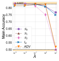
(a)

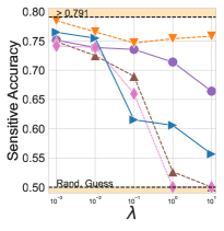
(b)

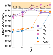
(c)

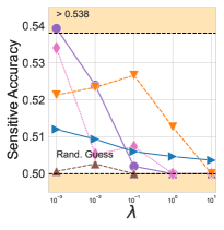
(d)

Fig. 2: Fair Classification results using BERT. Results are given with $B=256$ and $\tau_{p}=\tau_{n}=0.5$.

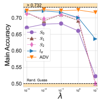
(a)

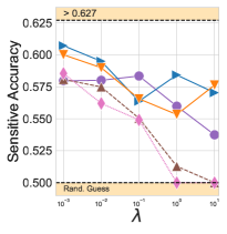
(b)

Fig. 3: Results on Fair Classification for a RNN.

Results on TRUST. This dataset exhibits an interesting behaviour known as spurious correlations Yule (1926); Simon (1954); Pearl et al. (2000). This means that, without any disentanglement penalty, the encoder learns information about the sensitive features that hurts the classification performance on the test set. We also observe that learning disentangled representation with CLINIC (using $S_{1}$ or $S_{2}$) outperforms a model trained with CE loss solely. This suggests that CLINIC could go beyond the standard disentanglement/accuracy trade-off.

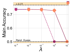
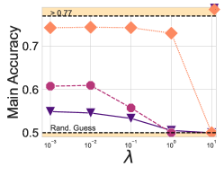
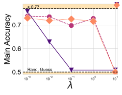
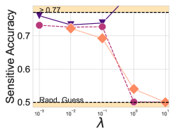
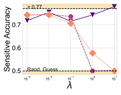
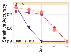
Fig. 4: Ablation study on PT on DIAL-S. Figures from
left to right correspond to the performance of ALB., DIS. and SEQU..

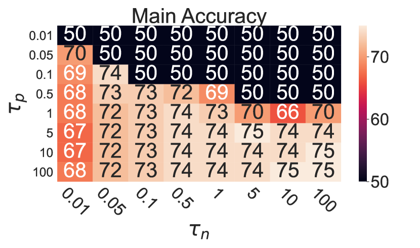
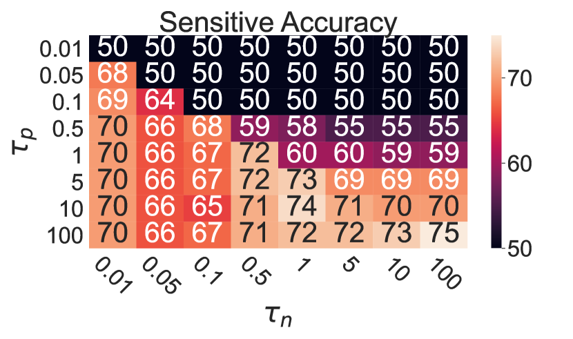
Fig. 5: Ablation study on $(\tau_{n},\tau_{p})$ for DIAL-S.

5.3 Superiority of the CLINIC’s Objective

In this experiment we assess the relevance of using $I(Z;S|Y)$ (Eq. 4) instead of $I(Z;S)$ (Eq. 3). For all the considered $\lambda$, all datasets and all the considered checkpoints, we display in Fig. 6 the disentanglement/accuracy trade-off.

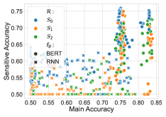
Fig. 6: Disentanglement/accuracy trade-off for various datasets, checkpoints and values of $\lambda$. Point with high sensitive accuracy (e.g. in the upper right corner) corresponds to low values of $\lambda$ (e.g. $\lambda\in\{10^{-3},10^{-2},10^{-1}\})$.

Analysis. Each point in Fig. 6 corresponds to a trained model (with a specific $\lambda$). The more a point is at the bottom right, the better it is for our purpose. Notice that the points stemming from our strategies $\mathcal{S}_{1}$ and $\mathcal{S}_{2}$ (orange/green) lie further down on the right than the point stemming from $\mathcal{S}_{0}$ (bleu). For instance, the use of $\mathcal{S}_{1}$ or $\mathcal{S}_{2}$ for the RNN provide many models exhibiting perfect sensitive accuracy while maintaining high main accuracy, which is not the case for $\mathcal{S}_{0}$. For BERT, models trained with $\mathcal{S}_{0}$ either have high sensitive and main accuracy or low sensitive and main accuracy. On the contrary, there are points stemming from $\mathcal{S}_{1}$ or $\mathcal{S}_{2}$ that lies on the bottom right of Fig. 6. Overall, Fig. 6 validates the use of $I(Z;S|Y)$ instead of $I(Z;S)$.

5.4 Speed up Gain

In contrast with CLINIC, both previous methods ADV and $I_{\alpha}$ rely on an additional network for the computation of the disentanglement regularizer in Eq. 1. These extra parameters need to be learned with the use of an additional loop during training: at each update of the encoder $f_{\theta}$, several updates of the network are performed to ensure that the regularizer computes the correct value. This loop is both times consuming and involves extra parameters (e.g new learning rates for the additional network) that must be tuned carefully. This makes ADV and $I_{\alpha}$ more difficult to implement on large-scale datasets. Tab. 2, illustrates both the parameter reduction and the speed up induced by CLINIC.

	Method	# params.	1 epoch.
RNN	ADV	2220 $-0.6\%$	551 $-17\%$
	$I_{\alpha}$	2234	663
	CLINIC	2206 $-1.3\%$	500 $-24\%$
BERT	ADV	109576 $-0.01\%$	2424 $-10\%$
	$I_{\alpha}$	109591	2689
	CLINIC	109576 $-0.03\%$	2200 $-19\%$

Tab. 2: Runtime for 1 epoch (using DIAL-S, $B=64$ and relying on a single NVIDIA-V100 with 32GB of memory). The model sizes are given in thousand. We compute the relative improvement with respect to the strongest baseline $I_{\alpha}$ from Colombo et al. (2021c).

6 Ablation Study

In this section, we conduct an ablation study on CLINIC with the best sampling strategy ($\mathcal{S}_{1}$) to better understand the importance of its relative components. We focus on the effect of (i) the choice of PT models, (ii) the batch size and (iii) the temperature. This ablation study is conducted for both DIAL-S and TRUST-A, where we recall that the former is harder to disentangle than the latter. Results on TRUST-A can be found in Ap. A.

6.1 Changing the PT Model

Setting. As recently pointed out by Bommasani et al. (2021), PT plays a central role in NLP, thus the need to understand their effects is crucial. We test CLINIC with PT that are lighter and require less computation time to finetune than BERT.
Analysis. The results of CLINIC trained with SQU., DIS. and ALB. are given in Fig. 5. Overall, we observe that CLINIC consistently achieves better results on all the considered models. Interestingly, for $\lambda>0.1$, we observe that ADV degenerates: the main task accuracy is around 50% and the sensitive task accuracy either is 50% or reaches a high value. This phenomenon has been reported in Barrett et al. (2019); Colombo et al. (2021c).

6.2 Effect of the Temperature

Recall that CLINIC uses two different temperatures (see Eq. 5) denoted by $\tau_{p}$ and $\tau_{n}$, corresponding to the magnitude one wishes to put on positive and negatives examples. In this experiment, we study their relative importance on the disentanglement/accuracy trade-off.
Analysis. Fig. 5 gathers the performance of CLINIC for different $(\tau_{p},\tau_{n})$. We observe that low values of $\tau_{p}$ (i.e focusing on easy positive) conduct to uninformative representation (i.e low accuracy for $Y$). As $\tau_{p}$ increases, the choice of $\tau_{n}$ becomes relevant. Previously introduced supervised contrastive losses Khosla et al. (2020) only use one temperature thus can only rely on diagonal score from Fig. 5. Since the chosen trade-off depends on the final application, we believe this ablation study validates the use of two temperatures.

7 Summary and Concluding Remarks

We introduced CLINIC, a set of novel losses tailored for fair classification. CLINIC both outperform existing disentanglement methods and can go beyond the traditional accuracy/disentanglement trade-off. Future works include (1) improving CLINIC to enable finer control over the disentanglement degree, and (2) developing a way to measure the accuracy/disentanglement trade-off which appears to differ for each dataset.

8 Limitations

This paper proposes a novel information-theoretic objective to learn disentangled representations. While the results held for English and studied pre-trained encoders, we observed different behavior depending on the disentanglement difficulty. Overall predicting for which attribute or which data we will be able to see a positive trade-off while disentangling remains an open question.

Additionally, similarly to previous work in the same line of research we also assumed to have access to $S$ which might not be the case for various practical applications. Note that although the main paper focuses on binary attributes for $S$ we report additional results in Ssec. A.1. In general, we believe that our embeddings could be utilized for diverse applications, such as sentence generation and large language models. However, evaluating their performance on these specific tasks falls beyond the scope of this paper. Future research should focus on addressing these aspects.

.1 Additional Motivation

We provide in Fig. 7 example of extreme situations when learning to disentangle representations. This figure can be analyzed using the Veyne diagram of Fig. 1.

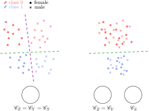
Fig. 7: Two extremes situations. In both cases, a classifier can predict the main task with high accuracy. The right representation is fairer than the left one as the gender is harder to extract.

Note that using MI is orthogonal to the work of INLP Ravfogel et al. (2020) as this works focus on linear null space projection. This has been extensively studied subramanian2021evaluating but our loss is more generic as it also accounts for non linear dependencies.

.2 Algorithms used for the baseline models.

When training an adversary or a MI with learnable parameters the procedure requires extra learnable parameters that need to be tuned using a Nested Loop.

Algorithm 1 Procedure to learn the baselines

1:Input Labeled dataset $\mathcal{D}=\{(x_{j},s_{j},y_{j}),\forall j\in[1,|\mathcal{D}|-K]\}$, independant labeled dataset $\mathcal{D^{\prime}}=\{(x_{j},s_{j},y_{j}),\forall j\in[|\mathcal{D}|-K,|\mathcal{D}|]\}$, $\theta$ parameters of the encoder network, $\phi$ parameters of the main classifier, $\psi$ parameters of the regularizer.

2:Initialize parameters $\theta$, $\phi$, $\psi$

3:Optimization

4:Freeze $\theta$

5:while $(\theta,\phi,\psi)$ not converged do

6:     for  $i\in[1,Unroll]$ do $\triangleright$ Nested loop

7:         Sample a batch $\mathcal{B^{\prime}}$ from $\mathcal{D^{\prime}}$

8:         Update $\phi,\psi$ using (Eq. 1).

9:     end for

10:     Unfreeze $\theta$ and freeze $\phi,\psi$

11:     Sample a batch $\mathcal{B}$ from $\mathcal{D}$

12:     Update $\theta$ with $\mathcal{B}$ (Eq. 1).

13:     Unfreeze $\phi,\psi$

14:end while

15:Output Encoder and classifier weights ${\theta,\phi}$

Appendix A Additional Experimental Results

In this section, we report additional experiments. Specifically, we gather:

• We report aditionnal baselines (see Ssec. A.1).

• All the unreported experiments in the core paper for fair classification task on both RNN and BERT for the four considered sensitive/main attribute pairs (see Ssec. A.3 for TRUST and Ssec. A.2 for DIAL).

• The ablation study on the PT choice for TRUST-G (see Sssec. A.4.2).

• The ablation study on the batch size for TRUST-G (see Sssec. A.4.1).

• The ablation study on the impact of the temperature for TRUST-G (see Sssec. A.4.3).

A.1 Additional Baseline

We run additional experiments and add 6 datasets and compare with recent work ADS from Chowdhury et al. (2021) on BERT. Please note that Chowdhury et al. (2021) is not really a concurrent work; they also use a CE term that we could replace. In fact, we can combine our objective with ADS. ADS stands for the work from Chowdhury et al. (2021) and ADS + CLINIC stands for ADS where the CE term has been replaced with our proposed objective (i.e., $I(S;Z|Y)$).

Considered Datasets To ensure backward comparisons with Chowdhury et al. (2021) . We additionally add results on FUNPEDIA Dinan et al. (2020), LIGHT Dinan et al. (2020), CONVAI2 Dinan et al. (2020), Wizzard Dinan et al. (2020), BIOGRAPHIES De-Arteaga et al. (2019). Note that theses results extends multiclass classification setting of the main paper.

Observations: From Tab. 3, Tab. 4, Tab. 5, Tab. 6, Tab. 7, Tab. 8, Tab. 9, Tab. 10, Tab. 11. We observe that CLINIC alone outperforms all other baselines on 6 out of 10 configurations. On the 4 remaining CLINIC improve over the work from Chowdhury et al. (2021) and CLINIC+Chowdhury et al. (2021) is SOTA on the 4 configurations. On Trust Pilot we do not see the improvement. This is likely due to the cross entropy. Which further illustrates the point of this paper. That we should go for the objective instead of the MI/CE.

Takeaways: Overall, CLINIC is both theoretically grounded and achieves strong results on over 10 datasets.

	AccY	F1S
RANDOM	50	50
VANILLA	76.2	76.7
ADV	73.5	72.9
CLINIC	73.5	58.3
ADS	74.5	60.0
ADS+CLINIC	74.5	57.0

Tab. 3: Additional Results on DIAL

	AccY	F1S
RANDOM	50	50
VANILLA	82.7	79.1
ADV	82.6	74.6
CLINIC	75.0	50.0
ADS	73.5	64.0
ADS+CLINIC	75.5	50.0

Tab. 4: Additional Results on DIAL

	AccY	F1S
RANDOM	50	50
VANILLA	74.9	53.8
ADV	70.1	50.0
CLINIC	75.1	50.0
ADS	70.3	50.0
ADS+CLINIC	75.8	50.0

Tab. 5: Additional Results on TRUST

	AccY	F1S
RANDOM	50	50
Vanilla	74.9	53.8
AD	73.2	50.0
CLINIC	76.2	50.0
> ADS	73.5	50.0
ADS+CLINIC	76.2	50.0

Tab. 6: Additional Results on TRUST

	AccY	F1S
RANDOM	33	33
VANILLA	94.0	55.9
ADV	64.1	47.0
CLINIC	93.1	33.0
ADS	90.3	34.0
ADS+CLINIC	91.4	33.8

Tab. 7: Additional Results on FUNPEDIA

	AccY	F1S
RANDOM	50	33
VANILLA	95.6	73.4
ADV|95.6	58.0
CLINIC	94.1	51.0
ADS	95.1	56.0
ADS+CLINIC	95.0	50.0

Tab. 8: Additional Results on ConvAI2

	AccY	F1S
RANDOM	50	33
VANILLA	91.4	73.5
ADV	91.1	60.0
CLINIC	91.4	51.0
ADS	91.1	53.0
ADS+CLINIC	91.3	52.0

Tab. 9: Additional Results on LIGHT

	AccY	F1S
RANDOM	50	33
VANILLA	85.1	70.3
ADV|88.1	64.0
CLINIC	94.5	50.0
ADS	94.0	50.0
ADS+CLINIC	95.8	50.0

Tab. 10: Additional Results on Wizard

	AccY	F1S
RANDOM	50	50
VANILLA	89.9	59.0
ADV	89.9	60.0
CLINIC	89.9	50.0
ADS	89.7	51.0
ADS+CLINIC	89.6	50.0

Tab. 11: Additional Results on PAN-AGE

A.2 Controlling experiment on DIAL

Important aspects when learning to disentangle representations are ($i$) achieving perfect independence between considered r.v while achieving high accuracy on the target task but also ($ii$) to control the desired level of disentanglement Feutry et al. (2018). To ease visual comparison, we report the results on the two main attributes mention (DIAL-M) and sentiment (DIAL-S) while protecting the race.
RNN-based encoder. We report in Fig. 8 the results of the RNN encoder on DIAL. We observe that for both cases, CLINIC is able to achieve perfect disentanglement. The loss $I_{\alpha}$ plateau for $\lambda\geq 0.1$. Overall the two best strategies ($\mathcal{S}_{1}$ and $\mathcal{S}_{2}$) achieve stronger results than considered baselines.
BERT-based encoder. For BERT we gather the results in Fig. 9. Similarly to what is reported in Ssec. 5.2, we observe a steep transition and notice that all considered estimators provide little control over the desired degree of disentanglement. It is worth noting that for DIAL-S, $\mathcal{S}_{2}$ underperforms and is not able to achieve better than 69.4 on the sensitive task accuracy. This failure case has motivated our choice for selecting $\mathcal{S}_{1}$ while conducting the ablation studies.

Takeaways. Overall, we observe that CLINIC outperforms considered baselines when combined with both RNN and BERT encoders on the DIAL dataset.

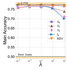
(a)

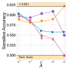
(b)

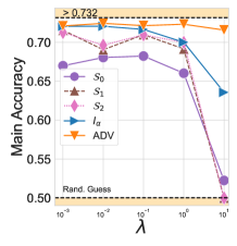
(c)

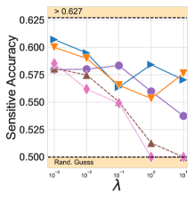
(d)

Fig. 8: Results on DIAL for the fair classification task relying on a RNN encoder.

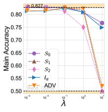
(a)

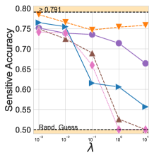
(b)

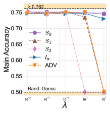
(c)

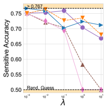
(d)

Fig. 9: Results on DIAL for the fair classification task using BERT.

A.3 Controlling experiment on TRUST

Here we report the results on TRUST for both attribute age (TRUST-A) and gender (TRUST-A) while predicting the sentiment on a like scale of 5.

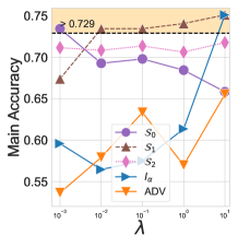
(a)

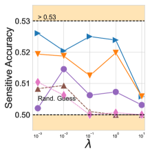
(b)

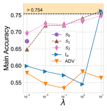
(c)

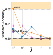
(d)

Fig. 10: Fair classification task on TRUST using a RNN encoder.

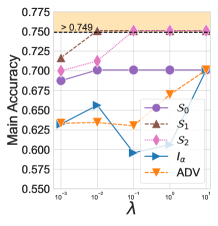
(a)

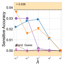
(b)

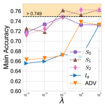
(c)

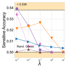
(d)

Fig. 11: Fair classification task results on TRUST with BERT.

RNN-based encoder. From Fig. 10, we observe that both attributes (i.e gender and age) can be disentangled from the main attribute (i.e sentiment label). Interestingly, we observe a general trend: the more the representations are disentangled (i.e the lower the sensitive accuracy) the higher accuracy is obtained on the main task. On both TRUST datasets, we observe that both CLINIC and $I_{\alpha}$ are able to outperform theCE model (reported by the upper dash line). Overall, most of the models are able to achieve almost perfectly disentangled representations, i.e for all models with $\lambda=10$ the sensitive accuracy falls below 51%.

BERT-based encoder. From Fig. 11, we observe similar trends to the previous ones: learning disentangled representation improves general performances on the main task. This phenomenon can be interpreted through the lens of spurious correlations Calude and Longo (2017). We observe that CLINIC with both $\mathcal{S}_{1}$ and $\mathcal{S}_{0}$ is able to remove almost all information from the sensitive labels even using small values of $\lambda$.

Takeaways. Overall on TRUST, it is easier to disentangle the representations from the sensitive attribute. We observe that CLINIC achieves strong results with both $\mathcal{S}_{1}$ and $\mathcal{S}_{2}$. It shows that incorporating the main label ($Y$) information in the sampling strategy for supervised contrastive learning loss is a key to achieve a good trade-off.

A.4 Additional results on ablation studies

In this section, we gather the results of the ablation studies conducted on CLINIC to better understand the relative importance of the different elements. We specifically report results on TRUST-A on the batch size (Sssec. A.4.1), the choice of the PT model (Sssec. A.4.2) as well as the role of the temperature (Sssec. A.4.3).

A.4.1 Effect of the batch size

Setting. As mentioned in Sec. 3, the batch size plays a key role when learning disentangled representations. In order to study its influence on CLINIC, we choose to work with DIS., to fit large batch sizes on a single GPU.

Analysis. We experiment with $\lambda=0.1$ and report the results on DIAL in Fig. 12. Interestingly, we observe a threshold phenomenon: for each model, a small value of the batch size leads to a poor performance on the main task. In contrast, working with large batch (i.e of size greater than 300) allows to learn representations that achieve low sensitive accuracy (around 57%) while maintaining a high main task accuracy (around 75%). On an easier task, changing the batch size does not impact the performances.

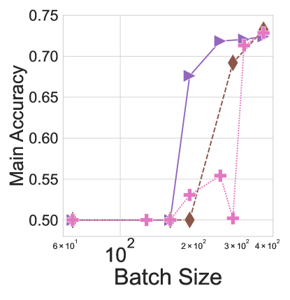
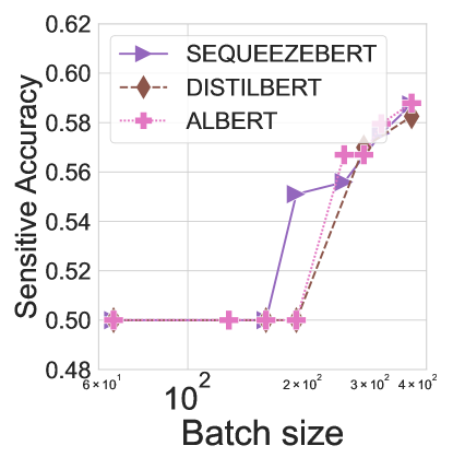
Fig. 12: Ablation on batch size on DIAL-S ($\lambda=1$).

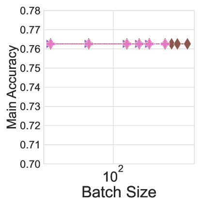
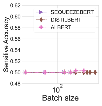
Fig. 13: Ablation study on batch size using DIS. for TRUST-A. Results on TRUST-G are given for $\lambda=1$.

A.4.2 Study on PT models

Fig. 14 gathers the results on the ablation study on PT for TRUST. We observe that for most of the considered PT, disentangling the representations improves the main task accuracy performance. We observe that overall CLINIC (with $\mathcal{S}_{1}$) achieves the best performances and can reach perfectly disentangled representations.

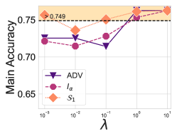
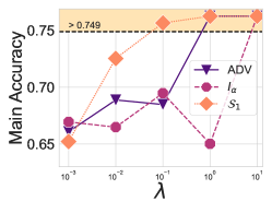
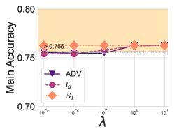
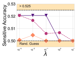
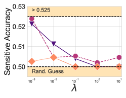
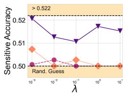
Fig. 14: Albation study on pretrained models on TRUST-A. Figures from left to right corresponds to the performance of ALB., DIS. and SQU. on TRUST-G.

Takeaways. When changing the pretrained model, we observe a consistent behavior of CLINIC which outperforms the considered baselines. The observe improvement when disentangling the representation is consistent across the different models which further validate the spurious correlation interpretation. This phenomenon is likely to be dataset and not model specific.

A.4.3 Study on temperature

We report on Fig. 15, the results of the ablation study on temperature conducted on TRUST-G. When the sensitive attribute is easier to disentangle, we observe that the sensitive accuracy is less impacted by a change in the temperature as most of the models achieve perfect disentanglement. However, there is an impact on the main task accuracy. Overall we observe some $(\tau_{n},\tau_{p})$ area achieving lower results (bottom right of the matrix Fig. 15).

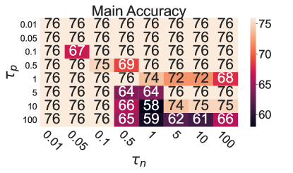
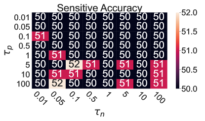
Fig. 15: Ablation study on $(\tau_{n},\tau_{p})$ for TRUST-A. Results are reported using BERT on TRUST-G for the main task $\uparrow$ (left) and the sensitive task $\downarrow$ (right) for $\lambda=0.1$ and $B=256$.

Takeaways. When working on TRUST that is easier to disentangle, we observe that the temperature tuning seems to have less impact on the sensitive task performance. However, it is needed to ensure a good sensitive/main task accuracy trade-off.

Appendix B Future Research Directions

In the future, we would like to explore the relationship between disentangled representations Colombo et al. (2022a); Darrin et al. (2023); Pichler et al. (2022); Colombo et al. (2021e, b, 2022d) learnt by encoder models Chapuis et al. (2020); Colombo et al. (2021a, d, 2019) and applications to anomaly detection (Staerman et al., 2019, 2020, 2021b; Staerman, 2022; Picot et al., 2022a, 2023; Colombo, 2021; Picot et al., 2022b; Darrin et al., 2022). Specifically, we are interested in benchmarking Colombo et al. (2022b, c); Staerman et al. (2021c) this in the scope of sentiment analysis Colombo et al. (2020); Jalalzai et al. (2020); Witon et al. (2018); Colombo et al. (2019); Garcia et al. (2019), conversational ai Dinkar et al. (2020), automatic metric evaluation Colombo et al. (2022e); Chhun et al. (2022), optimal transport (Staerman et al., 2021a; Laforgue et al., 2021; Colombo et al., 2021f) or transfer learning (Aghbalou and Staerman, 2023; Staerman et al., 2023).

Appendix C Training Details

We report in this section training details to reproduce the reported experiments. We give estimate run times on NVIDIA-V100 with 32Go of memory.

C.1 Model architecture

We report in the section the considered model architectures.
RNN-encoder. For this model, we use a bidirectionnal GRU Chung et al. (2014) with 2 layers (the hidden dimension is set to 128) with LeakyReLU Xu et al. (2015). The encoder is followed by multi-layer perceptron of dimension 256.
Pretrained-encoder. For this model the encoder is followed by a single projection layer.
Attacker network. It is composed of 3 hidden layers with input sizes of $H_{dim}$, where $H_{dim}$ refers to the dimension of the attacked network.

C.2 Implementation details

All the models have been trained using the ADAMW optimizer Loshchilov and Hutter (2017) which is an improvement of the ADAM Kingma and Ba (2014) optimizer with warmup set to 1000 Vaswani et al. (2017). The dropout rate Srivastava et al. (2014) has been set to 0.2. The learning rate of the optimizer has been set to 0.001 for the RNN-based encoders and to 0.00001 for the BERT models. The PT are trained for 15k iterations and the randomly initialized RNN are trained for 30k iterations.

Used libraries. In this work we relied on the following libraries and would like to thank their authors for open-sourcing them:

• Code from Barrett et al. (2019); Elazar and Goldberg (2018) to process DIAL. The baseline ADV has been re-implemented in our framework. The associated Github can be found https://github.com/yanaiela/demog-text-removal.

• Code from Coavoux et al. (2018) to process DI. In their work they also used the ADV baseline has been re-implemented in our framework. The associated GitHub can be found here: https://github.com/mcoavoux/pnet.

• Code from Colombo et al. (2021c) has been privately shared by the authors.

• All the models have been implemented in Pytorch Paszke et al. (2017).

• The tokenizers, the PT have been taken from transformers Wolf et al. .

C.3 Computing costs

In this section, we report the (estimated) computational cost of reproducing our experiments. Note that we relieved on NVIDIA-V100 with 32 GO of memory. Each pretrained model takes (approximately) 3 hours to train and whereas the RNN encoder requires 5 hours to be trained. All models have been trained with batch size of 256. An adversary requires around 15 mins to be trained. Controlling experiment. For this experiments we trained $5\times 5\times 4=100$ RNN encoders and the same number of pretrained models. For each model we evaluate 6 checkpoints which makes 1200 probing classifiers. The checkpoint with lowest $\mathcal{R}$ (see Eq. 1) is selected. This experiment requires $500+300+1200/4=1100h$ of GPUs.

Ablation study. For the batch size experiment, we trained $8\times 3\times 2=48$ models with 240 probing classifiers for a total cost of GPU 204 hours. For the pretrained models ablation study, we trained $5\times 3\times 2=30$ models with 150 probing classifiers for a total cost of 128 hours. For the temperature we trained $8\times 8\times 2=128$ models with 640 probing classifiers for a total of 544 GPU hours.

Overall summary. The approximated total cost is around 2k GPU hours.

References

- Aghbalou and Staerman (2023) Anass Aghbalou and Guillaume Staerman. 2023. Hypothesis transfer learning with surrogate classification losses. arXiv preprint arXiv:2305.19694.
- Ahn and Oh (2021) Jaimeen Ahn and Alice Oh. 2021. Mitigating language-dependent ethnic bias in bert. arXiv preprint arXiv:2109.05704.
- Bachman et al. (2019) Philip Bachman, R Devon Hjelm, and William Buchwalter. 2019. Learning representations by maximizing mutual information across views. arXiv preprint arXiv:1906.00910.
- Barrett et al. (2019) Maria Barrett, Yova Kementchedjhieva, Yanai Elazar, Desmond Elliott, and Anders Søgaard. 2019. Adversarial removal of demographic attributes revisited. In Proceedings of the 2019 Conference on Empirical Methods in Natural Language Processing and the 9th International Joint Conference on Natural Language Processing (EMNLP-IJCNLP), pages 6331–6336.
- Belghazi et al. (2018) Mohamed Ishmael Belghazi, Aristide Baratin, Sai Rajeswar, Sherjil Ozair, Yoshua Bengio, Aaron Courville, and R Devon Hjelm. 2018. Mine: mutual information neural estimation. arXiv preprint arXiv:1801.04062.
- Bengio et al. (2013) Y. Bengio, A. Courville, and P. Vincent. 2013. Representation learning: A review and new perspectives. IEEE Transactions on Pattern Analysis and Machine Intelligence, 35(8):1798–1828.
- Blodgett et al. (2016) Su Lin Blodgett, Lisa Green, and Brendan O’Connor. 2016. Demographic dialectal variation in social media: A case study of African-American English. In Proceedings of the 2016 Conference on Empirical Methods in Natural Language Processing, pages 1119–1130, Austin, Texas.
- Bommasani et al. (2021) Rishi Bommasani, Drew A Hudson, Ehsan Adeli, Russ Altman, Simran Arora, Sydney von Arx, Michael S Bernstein, Jeannette Bohg, Antoine Bosselut, Emma Brunskill, et al. 2021. On the opportunities and risks of foundation models. arXiv preprint arXiv:2108.07258.
- Brunet et al. (2019) Marc-Etienne Brunet, Colleen Alkalay-Houlihan, Ashton Anderson, and Richard Zemel. 2019. Understanding the origins of bias in word embeddings. In International Conference on Machine Learning, pages 803–811.
- Calude and Longo (2017) Cristian S Calude and Giuseppe Longo. 2017. The deluge of spurious correlations in big data. Foundations of science, 22(3):595–612.
- Caton and Haas (2020) Simon Caton and Christian Haas. 2020. Fairness in machine learning: A survey. arXiv preprint arXiv:2010.04053.
- Chapuis et al. (2020) Emile Chapuis, Pierre Colombo, Matteo Manica, Matthieu Labeau, and Chloé Clavel. 2020. Hierarchical pre-training for sequence labelling in spoken dialog. In Findings of the Association for Computational Linguistics: EMNLP 2020, pages 2636–2648, Online. Association for Computational Linguistics.
- Chen et al. (2020) Ting Chen, Simon Kornblith, Mohammad Norouzi, and Geoffrey Hinton. 2020. A simple framework for contrastive learning of visual representations. In International conference on machine learning, pages 1597–1607.
- Cheng et al. (2020) Pengyu Cheng, Weituo Hao, Shuyang Dai, Jiachang Liu, Zhe Gan, and Lawrence Carin. 2020. Club: A contrastive log-ratio upper bound of mutual information. In International Conference on Machine Learning, pages 1779–1788.
- Chhun et al. (2022) Cyril Chhun, Pierre Colombo, Fabian M. Suchanek, and Chloé Clavel. 2022. Of human criteria and automatic metrics: A benchmark of the evaluation of story generation. In Proceedings of the 29th International Conference on Computational Linguistics, pages 5794–5836, Gyeongju, Republic of Korea. International Committee on Computational Linguistics.
- Chi et al. (2022) Jianfeng Chi, William Shand, Yaodong Yu, Kai-Wei Chang, Han Zhao, and Yuan Tian. 2022. Conditional supervised contrastive learning for fair text classification. arXiv preprint arXiv:2205.11485.
- Chopra et al. (2005) Sumit Chopra, Raia Hadsell, and Yann LeCun. 2005. Learning a similarity metric discriminatively, with application to face verification. In 2005 IEEE Computer Society Conference on Computer Vision and Pattern Recognition (CVPR’05), volume 1, pages 539–546.
- Chowdhury et al. (2021) Somnath Basu Roy Chowdhury, Sayan Ghosh, Yiyuan Li, Junier B Oliva, Shashank Srivastava, and Snigdha Chaturvedi. 2021. Adversarial scrubbing of demographic information for text classification. arXiv preprint arXiv:2109.08613.
- Chung et al. (2014) Junyoung Chung, Caglar Gulcehre, KyungHyun Cho, and Yoshua Bengio. 2014. Empirical evaluation of gated recurrent neural networks on sequence modeling. arXiv preprint arXiv:1412.3555.
- Coavoux et al. (2018) Maximin Coavoux, Shashi Narayan, and Shay B Cohen. 2018. Privacy-preserving neural representations of text. arXiv preprint arXiv:1808.09408.
- Colombo (2021) Pierre Colombo. 2021. Learning to represent and generate text using information measures. Ph.D. thesis, Institut polytechnique de Paris.
- Colombo et al. (2021a) Pierre Colombo, Emile Chapuis, Matthieu Labeau, and Chloé Clavel. 2021a. Code-switched inspired losses for spoken dialog representations. In Proceedings of the 2021 Conference on Empirical Methods in Natural Language Processing, pages 8320–8337, Online and Punta Cana, Dominican Republic. Association for Computational Linguistics.
- Colombo et al. (2021b) Pierre Colombo, Emile Chapuis, Matthieu Labeau, and Chloé Clavel. 2021b. Improving multimodal fusion via mutual dependency maximisation. In Proceedings of the 2021 Conference on Empirical Methods in Natural Language Processing, pages 231–245, Online and Punta Cana, Dominican Republic. Association for Computational Linguistics.
- Colombo et al. (2020) Pierre Colombo, Emile Chapuis, Matteo Manica, Emmanuel Vignon, Giovanna Varni, and Chloe Clavel. 2020. Guiding attention in sequence-to-sequence models for dialogue act prediction. In AAAI, pages 7594–7601.
- Colombo et al. (2021c) Pierre Colombo, Chloe Clavel, and Pablo Piantanida. 2021c. A novel estimator of mutual information for learning to disentangle textual representations. arXiv preprint arXiv:2105.02685.
- Colombo et al. (2021d) Pierre Colombo, Chloé Clavel, Chouchang Yack, and Giovanna Varni. 2021d. Beam search with bidirectional strategies for neural response generation. In Proceedings of the 4th International Conference on Natural Language and Speech Processing (ICNLSP 2021), pages 139–146, Trento, Italy. Association for Computational Linguistics.
- Colombo et al. (2022a) Pierre Colombo, Eduardo Dadalto, Guillaume Staerman, Nathan Noiry, and Pablo Piantanida. 2022a. Beyond mahalanobis distance for textual ood detection. In Advances in Neural Information Processing Systems, volume 35, pages 17744–17759. Curran Associates, Inc.
- Colombo et al. (2022b) Pierre Colombo, Nathan Noiry, Ekhine Irurozki, and Stéphan Clémençon. 2022b. What are the best systems? new perspectives on nlp benchmarking. Advances in Neural Information Processing Systems, 35:26915–26932.
- Colombo et al. (2022c) Pierre Colombo, Maxime Peyrard, Nathan Noiry, Robert West, and Pablo Piantanida. 2022c. The glass ceiling of automatic evaluation in natural language generation. arXiv preprint arXiv:2208.14585.
- Colombo et al. (2021e) Pierre Colombo, Pablo Piantanida, and Chloé Clavel. 2021e. A novel estimator of mutual information for learning to disentangle textual representations. In Proceedings of the 59th Annual Meeting of the Association for Computational Linguistics and the 11th International Joint Conference on Natural Language Processing (Volume 1: Long Papers), pages 6539–6550, Online. Association for Computational Linguistics.
- Colombo et al. (2021f) Pierre Colombo, Guillaume Staerman, Chloé Clavel, and Pablo Piantanida. 2021f. Automatic text evaluation through the lens of Wasserstein barycenters. In Proceedings of the 2021 Conference on Empirical Methods in Natural Language Processing, pages 10450–10466, Online and Punta Cana, Dominican Republic. Association for Computational Linguistics.
- Colombo et al. (2022d) Pierre Colombo, Guillaume Staerman, Nathan Noiry, and Pablo Piantanida. 2022d. Learning disentangled textual representations via statistical measures of similarity. In Proceedings of the 60th Annual Meeting of the Association for Computational Linguistics (Volume 1: Long Papers), pages 2614–2630, Dublin, Ireland. Association for Computational Linguistics.
- Colombo et al. (2019) Pierre Colombo, Wojciech Witon, Ashutosh Modi, James Kennedy, and Mubbasir Kapadia. 2019. Affect-driven dialog generation. In Proceedings of the 2019 Conference of the North American Chapter of the Association for Computational Linguistics: Human Language Technologies, Volume 1 (Long and Short Papers), pages 3734–3743, Minneapolis, Minnesota. Association for Computational Linguistics.
- Colombo et al. (2022e) Pierre Jean A. Colombo, Chloé Clavel, and Pablo Piantanida. 2022e. Infolm: A new metric to evaluate summarization & data2text generation. Proceedings of the AAAI Conference on Artificial Intelligence, 36(10):10554–10562.
- Cover and Thomas (2006) Thomas M. Cover and Joy A. Thomas. 2006. Elements of Information Theory (Wiley Series in Telecommunications and Signal Processing). Wiley-Interscience, USA.
- d’Alessandro et al. (2017) Brian d’Alessandro, Cathy O’Neil, and Tom LaGatta. 2017. Conscientious classification: A data scientist’s guide to discrimination-aware classification. Big data, 5(2):120–134.
- Darrin et al. (2022) Maxime Darrin, Pablo Piantanida, and Pierre Colombo. 2022. Rainproof: An umbrella to shield text generators from out-of-distribution data. arXiv preprint arXiv:2212.09171.
- Darrin et al. (2023) Maxime Darrin, Guillaume Staerman, Eduardo Dadalto Câmara Gomes, Jackie CK Cheung, Pablo Piantanida, and Pierre Colombo. 2023. Unsupervised layer-wise score aggregation for textual ood detection. arXiv preprint arXiv:2302.09852.
- De-Arteaga et al. (2019) Maria De-Arteaga, Alexey Romanov, Hanna Wallach, Jennifer Chayes, Christian Borgs, Alexandra Chouldechova, Sahin Geyik, Krishnaram Kenthapadi, and Adam Tauman Kalai. 2019. Bias in bios: A case study of semantic representation bias in a high-stakes setting. In proceedings of the Conference on Fairness, Accountability, and Transparency, pages 120–128.
- de Vassimon Manela et al. (2021) Daniel de Vassimon Manela, David Errington, Thomas Fisher, Boris van Breugel, and Pasquale Minervini. 2021. Stereotype and skew: Quantifying gender bias in pre-trained and fine-tuned language models. In Proceedings of the 16th Conference of the European Chapter of the Association for Computational Linguistics: Main Volume, pages 2232–2242.
- Devlin et al. (2018) Jacob Devlin, Ming-Wei Chang, Kenton Lee, and Kristina Toutanova. 2018. Bert: Pre-training of deep bidirectional transformers for language understanding. arXiv preprint arXiv:1810.04805.
- Dinan et al. (2020) Emily Dinan, Angela Fan, Ledell Wu, Jason Weston, Douwe Kiela, and Adina Williams. 2020. Multi-dimensional gender bias classification. arXiv preprint arXiv:2005.00614.
- Dinkar et al. (2020) Tanvi Dinkar, Pierre Colombo, Matthieu Labeau, and Chloé Clavel. 2020. The importance of fillers for text representations of speech transcripts. In Proceedings of the 2020 Conference on Empirical Methods in Natural Language Processing (EMNLP), pages 7985–7993, Online. Association for Computational Linguistics.
- Elazar and Goldberg (2018) Yanai Elazar and Yoav Goldberg. 2018. Adversarial removal of demographic attributes from text data. arXiv preprint arXiv:1808.06640.
- Fang et al. (2020) Hongchao Fang, Sicheng Wang, Meng Zhou, Jiayuan Ding, and Pengtao Xie. 2020. Cert: Contrastive self-supervised learning for language understanding. arXiv preprint arXiv:2005.12766.
- Feutry et al. (2018) Clément Feutry, Pablo Piantanida, Yoshua Bengio, and Pierre Duhamel. 2018. Learning anonymized representations with adversarial neural networks. arXiv preprint arXiv:1802.09386.
- Gabbay and Hoshen (2019) Aviv Gabbay and Yedid Hoshen. 2019. Demystifying inter-class disentanglement. arXiv preprint arXiv:1906.11796.
- Gajane and Pechenizkiy (2017) Pratik Gajane and Mykola Pechenizkiy. 2017. On formalizing fairness in prediction with machine learning. arXiv preprint arXiv:1710.03184.
- Gao et al. (2021) Luyu Gao, Yunyi Zhang, Jiawei Han, and Jamie Callan. 2021. Scaling deep contrastive learning batch size under memory limited setup. In Proceedings of the 6th Workshop on Representation Learning for NLP (RepL4NLP-2021), pages 316–321.
- Garcia et al. (2019) Alexandre Garcia, Pierre Colombo, Florence d’Alché Buc, Slim Essid, and Chloé Clavel. 2019. From the token to the review: A hierarchical multimodal approach to opinion mining. In Proceedings of the 2019 Conference on Empirical Methods in Natural Language Processing and the 9th International Joint Conference on Natural Language Processing (EMNLP-IJCNLP), pages 5539–5548, Hong Kong, China. Association for Computational Linguistics.
- Gillick et al. (2019) Daniel Gillick, Sayali Kulkarni, Larry Lansing, Alessandro Presta, Jason Baldridge, Eugene Ie, and Diego Garcia-Olano. 2019. Learning dense representations for entity retrieval. arXiv preprint arXiv:1909.10506.
- Giorgi et al. (2020) John M Giorgi, Osvald Nitski, Gary D Bader, and Bo Wang. 2020. Declutr: Deep contrastive learning for unsupervised textual representations. arXiv preprint arXiv:2006.03659.
- Gupta et al. (2021) Umang Gupta, Aaron M Ferber, Bistra Dilkina, and Greg Ver Steeg. 2021. Controllable guarantees for fair outcomes via contrastive information estimation. In Proceedings of the AAAI Conference on Artificial Intelligence, volume 35, pages 7610–7619.
- He et al. (2020) Kaiming He, Haoqi Fan, Yuxin Wu, Saining Xie, and Ross Girshick. 2020. Momentum contrast for unsupervised visual representation learning. In Proceedings of the IEEE/CVF Conference on Computer Vision and Pattern Recognition, pages 9729–9738.
- Henaff (2020) Olivier Henaff. 2020. Data-efficient image recognition with contrastive predictive coding. In International Conference on Machine Learning, pages 4182–4192. PMLR.
- Hovy et al. (2015) Dirk Hovy, Anders Johannsen, and Anders Søgaard. 2015. User review sites as a resource for large-scale sociolinguistic studies. In Proceedings of the 24th international conference on World Wide Web, pages 452–461.
- Hovy and Søgaard (2015) Dirk Hovy and Anders Søgaard. 2015. Tagging performance correlates with author age. In Proceedings of the 53rd annual meeting of the Association for Computational Linguistics and the 7th international joint conference on natural language processing (volume 2: Short papers), pages 483–488.
- Iandola et al. (2020) Forrest N Iandola, Albert E Shaw, Ravi Krishna, and Kurt W Keutzer. 2020. Squeezebert: What can computer vision teach nlp about efficient neural networks? arXiv preprint arXiv:2006.11316.
- Jalalzai et al. (2020) Hamid Jalalzai, Pierre Colombo, Chloé Clavel, Eric Gaussier, Giovanna Varni, Emmanuel Vignon, and Anne Sabourin. 2020. Heavy-tailed representations, text polarity classification & data augmentation. In Advances in Neural Information Processing Systems, volume 33, pages 4295–4307. Curran Associates, Inc.
- John et al. (2018) Vineet John, Lili Mou, Hareesh Bahuleyan, and Olga Vechtomova. 2018. Disentangled representation learning for non-parallel text style transfer. arXiv preprint arXiv:1808.04339.
- Kamiran and Calders (2012) Faisal Kamiran and Toon Calders. 2012. Data preprocessing techniques for classification without discrimination. Knowledge and Information Systems, 33(1):1–33.
- Karpukhin et al. (2020) Vladimir Karpukhin, Barlas Oğuz, Sewon Min, Patrick Lewis, Ledell Wu, Sergey Edunov, Danqi Chen, and Wen-tau Yih. 2020. Dense passage retrieval for open-domain question answering. arXiv preprint arXiv:2004.04906.
- Khosla et al. (2020) Prannay Khosla, Piotr Teterwak, Chen Wang, Aaron Sarna, Yonglong Tian, Phillip Isola, Aaron Maschinot, Ce Liu, and Dilip Krishnan. 2020. Supervised contrastive learning. arXiv preprint arXiv:2004.11362.
- Kingma and Ba (2014) Diederik P Kingma and Jimmy Ba. 2014. Adam: A method for stochastic optimization. arXiv preprint arXiv:1412.6980.
- Laforgue et al. (2021) Pierre Laforgue, Guillaume Staerman, and Stephan Clémençon. 2021. Generalization bounds in the presence of outliers: a median-of-means study. In International Conference on Machine Learning, pages 5937–5947. PMLR.
- Lample et al. (2018) Guillaume Lample, Sandeep Subramanian, Eric Smith, Ludovic Denoyer, Marc’Aurelio Ranzato, and Y-Lan Boureau. 2018. Multiple-attribute text rewriting. In International Conference on Learning Representations.
- Lan et al. (2019) Zhenzhong Lan, Mingda Chen, Sebastian Goodman, Kevin Gimpel, Piyush Sharma, and Radu Soricut. 2019. Albert: A lite bert for self-supervised learning of language representations. arXiv preprint arXiv:1909.11942.
- Lipton et al. (2018) Zachary C Lipton, Alexandra Chouldechova, and Julian McAuley. 2018. Does mitigating ml’s impact disparity require treatment disparity? In Proceedings of the 32nd International Conference on Neural Information Processing Systems, pages 8136–8146.
- Locatello et al. (2019a) Francesco Locatello, Gabriele Abbati, Tom Rainforth, Stefan Bauer, Bernhard Schölkopf, and Olivier Bachem. 2019a. On the fairness of disentangled representations. arXiv preprint arXiv:1905.13662.
- Locatello et al. (2019b) Francesco Locatello, Stefan Bauer, Mario Lucic, Gunnar Raetsch, Sylvain Gelly, Bernhard Schölkopf, and Olivier Bachem. 2019b. Challenging common assumptions in the unsupervised learning of disentangled representations. In international conference on machine learning, pages 4114–4124.
- Locatello et al. (2020) Francesco Locatello, Stefan Bauer, Mario Lucic, Gunnar Rätsch, Sylvain Gelly, Bernhard Schölkopf, and Olivier Bachem. 2020. A sober look at the unsupervised learning of disentangled representations and their evaluation. arXiv preprint arXiv:2010.14766.
- Logeswaran and Lee (2018) Lajanugen Logeswaran and Honglak Lee. 2018. An efficient framework for learning sentence representations. arXiv preprint arXiv:1803.02893.
- Loshchilov and Hutter (2017) Ilya Loshchilov and Frank Hutter. 2017. Decoupled weight decay regularization. arXiv preprint arXiv:1711.05101.
- Mathieu et al. (2019) Emile Mathieu, Tom Rainforth, Nana Siddharth, and Yee Whye Teh. 2019. Disentangling disentanglement in variational autoencoders. In International Conference on Machine Learning, pages 4402–4412.
- McAllester and Stratos (2020) David McAllester and Karl Stratos. 2020. Formal limitations on the measurement of mutual information. In Proceedings of the Twenty Third International Conference on Artificial Intelligence and Statistics, volume 108 of Proceedings of Machine Learning Research, pages 875–884.
- Mitrovic et al. (2020) Jovana Mitrovic, Brian McWilliams, and Melanie Rey. 2020. Less can be more in contrastive learning.
- Mozafari et al. (2020) Marzieh Mozafari, Reza Farahbakhsh, and Noël Crespi. 2020. Hate speech detection and racial bias mitigation in social media based on bert model. PloS one, 15(8):e0237861.
- Nguyen et al. (2010) XuanLong Nguyen, Martin J Wainwright, and Michael I Jordan. 2010. Estimating divergence functionals and the likelihood ratio by convex risk minimization. IEEE Transactions on Information Theory.
- Oord et al. (2018) Aaron van den Oord, Yazhe Li, and Oriol Vinyals. 2018. Representation learning with contrastive predictive coding. arXiv preprint arXiv:1807.03748.
- Paninski (2003) Liam Paninski. 2003. Estimation of entropy and mutual information. Neural computation, 15(6):1191–1253.
- Paszke et al. (2017) Adam Paszke, Sam Gross, Soumith Chintala, Gregory Chanan, Edward Yang, Zachary DeVito, Zeming Lin, Alban Desmaison, Luca Antiga, and Adam Lerer. 2017. Automatic differentiation in pytorch. In NIPS 2017 Workshop on Autodiff.
- Pearl et al. (2000) Judea Pearl et al. 2000. Models, reasoning and inference. Cambridge, UK: CambridgeUniversityPress, 19.
- Pichler et al. (2022) Georg Pichler, Pierre Jean A. Colombo, Malik Boudiaf, Günther Koliander, and Pablo Piantanida. 2022. A differential entropy estimator for training neural networks. In Proceedings of the 39th International Conference on Machine Learning, volume 162 of Proceedings of Machine Learning Research, pages 17691–17715. PMLR.
- Pichler et al. (2020) Georg Pichler, Pablo Piantanida, and Günther Koliander. 2020. On the estimation of information measures of continuous distributions. arXiv preprint arXiv:2002.02851.
- Picot et al. (2023) Marine Picot, Federica Granese, Guillaume Staerman, Marco Romanelli, Francisco Messina, Pablo Piantanida, and Pierre Colombo. 2023. A halfspace-mass depth-based method for adversarial attack detection. Transactions on Machine Learning Research.
- Picot et al. (2022a) Marine Picot, Nathan Noiry, Pablo Piantanida, and Pierre Colombo. 2022a. Adversarial attack detection under realistic constraints.
- Picot et al. (2022b) Marine Picot, Guillaume Staerman, Federica Granese, Nathan Noiry, Francisco Messina, Pablo Piantanida, and Pierre Colombo. 2022b. A simple unsupervised data depth-based method to detect adversarial images.
- Qian et al. (2021) Rui Qian, Tianjian Meng, Boqing Gong, Ming-Hsuan Yang, Huisheng Wang, Serge Belongie, and Yin Cui. 2021. Spatiotemporal contrastive video representation learning. In Proceedings of the IEEE/CVF Conference on Computer Vision and Pattern Recognition, pages 6964–6974.
- Qu et al. (2020) Yanru Qu, Dinghan Shen, Yelong Shen, Sandra Sajeev, Jiawei Han, and Weizhu Chen. 2020. Coda: Contrast-enhanced and diversity-promoting data augmentation for natural language understanding. arXiv preprint arXiv:2010.08670.
- Ravfogel et al. (2020) Shauli Ravfogel, Yanai Elazar, Hila Gonen, Michael Twiton, and Yoav Goldberg. 2020. Null it out: Guarding protected attributes by iterative nullspace projection. arXiv preprint arXiv:2004.07667.
- Reimers and Gurevych (2019) Nils Reimers and Iryna Gurevych. 2019. Sentence-bert: Sentence embeddings using siamese bert-networks. arXiv preprint arXiv:1908.10084.
- Rethmeier and Augenstein (2021) Nils Rethmeier and Isabelle Augenstein. 2021. A primer on contrastive pretraining in language processing: Methods, lessons learned and perspectives. arXiv preprint arXiv:2102.12982.
- Robinson et al. (2020) Joshua Robinson, Ching-Yao Chuang, Suvrit Sra, and Stefanie Jegelka. 2020. Contrastive learning with hard negative samples. arXiv preprint arXiv:2010.04592.
- Sanh et al. (2019) Victor Sanh, Lysandre Debut, Julien Chaumond, and Thomas Wolf. 2019. Distilbert, a distilled version of bert: smaller, faster, cheaper and lighter. arXiv preprint arXiv:1910.01108.
- Schroff et al. (2015) Florian Schroff, Dmitry Kalenichenko, and James Philbin. 2015. Facenet: A unified embedding for face recognition and clustering. In Proceedings of the IEEE conference on computer vision and pattern recognition, pages 815–823.
- Shen et al. (2021) Aili Shen, Xudong Han, Trevor Cohn, Timothy Baldwin, and Lea Frermann. 2021. Contrastive learning for fair representations. arXiv preprint arXiv:2109.10645.
- Shen et al. (2022) Aili Shen, Xudong Han, Trevor Cohn, Timothy Baldwin, and Lea Frermann. 2022. Does representational fairness imply empirical fairness? In Findings of the Association for Computational Linguistics: AACL-IJCNLP 2022, pages 81–95.
- Shen et al. (2020) Dinghan Shen, Mingzhi Zheng, Yelong Shen, Yanru Qu, and Weizhu Chen. 2020. A simple but tough-to-beat data augmentation approach for natural language understanding and generation. arXiv preprint arXiv:2009.13818.
- Simon (1954) Herbert A Simon. 1954. Spurious correlation: A causal interpretation. Journal of the American statistical Association, 49(267):467–479.
- Song and Ermon (2019) Jiaming Song and Stefano Ermon. 2019. Understanding the limitations of variational mutual information estimators. arXiv preprint arXiv:1910.06222.
- Sridhar et al. (2021) A Sridhar, Chawin Sitawarin, and David Wagner. 2021. Mitigating adversarial training instability with batch normalization. In Proceedings of International Conference on Learning Representation Workshop on Security and Safety in Machine Learning Systems.
- Srivastava et al. (2014) Nitish Srivastava, Geoffrey Hinton, Alex Krizhevsky, Ilya Sutskever, and Ruslan Salakhutdinov. 2014. Dropout: a simple way to prevent neural networks from overfitting. The journal of machine learning research, 15(1):1929–1958.
- Staerman (2022) Guillaume Staerman. 2022. Functional anomaly detection and robust estimation. Ph.D. thesis, Institut polytechnique de Paris.
- Staerman et al. (2023) Guillaume Staerman, Eric Adjakossa, Pavlo Mozharovskyi, Vera Hofer, Jayant Sen Gupta, and Stephan Clémençon. 2023. Functional anomaly detection: a benchmark study. International Journal of Data Science and Analytics, 16(16):101–117.
- Staerman et al. (2021a) Guillaume Staerman, Pierre Laforgue, Pavlo Mozharovskyi, and Florence d’Alché Buc. 2021a. When ot meets mom: Robust estimation of wasserstein distance. In Proceedings of The 24th International Conference on Artificial Intelligence and Statistics, volume 130, pages 136–144.
- Staerman et al. (2019) Guillaume Staerman, Pavlo Mozharovskyi, Stephan Clémençon, and Florence d’Alché Buc. 2019. Functional isolation forest. In Proceedings of The Eleventh Asian Conference on Machine Learning, volume 101, pages 332–347.
- Staerman et al. (2020) Guillaume Staerman, Pavlo Mozharovskyi, and Stéphan Clémençon. 2020. The area of the convex hull of sampled curves: a robust functional statistical depth measure. In Proceedings of the 23nd International Conference on Artificial Intelligence and Statistics, volume 108, pages 570–579.
- Staerman et al. (2021b) Guillaume Staerman, Pavlo Mozharovskyi, and Stéphan Clémençon. 2021b. Affine-invariant integrated rank-weighted depth: Definition, properties and finite sample analysis. arXiv preprint arXiv:2106.11068.
- Staerman et al. (2021c) Guillaume Staerman, Pavlo Mozharovskyi, Pierre Colombo, Stéphan Clémençon, and Florence d’Alché Buc. 2021c. A pseudo-metric between probability distributions based on depth-trimmed regions. arXiv preprint arXiv:2103.12711.
- Vaswani et al. (2017) Ashish Vaswani, Noam Shazeer, Niki Parmar, Jakob Uszkoreit, Llion Jones, Aidan N Gomez, Łukasz Kaiser, and Illia Polosukhin. 2017. Attention is all you need. In Advances in neural information processing systems, pages 5998–6008.
- Wang and Liu (2021) Feng Wang and Huaping Liu. 2021. Understanding the behaviour of contrastive loss. In Proceedings of the IEEE/CVF Conference on Computer Vision and Pattern Recognition, pages 2495–2504.
- Wang and Isola (2020) Tongzhou Wang and Phillip Isola. 2020. Understanding contrastive representation learning through alignment and uniformity on the hypersphere. In International Conference on Machine Learning, pages 9929–9939.
- Witon et al. (2018) Wojciech Witon, Pierre Colombo, Ashutosh Modi, and Mubbasir Kapadia. 2018. Disney at IEST 2018: Predicting emotions using an ensemble. In Proceedings of the 9th Workshop on Computational Approaches to Subjectivity, Sentiment and Social Media Analysis, pages 248–253, Brussels, Belgium. Association for Computational Linguistics.
- (114) Thomas Wolf, Lysandre Debut, Victor Sanh, Julien Chaumond, Clement Delangue, Anthony Moi, Pierric Cistac, Tim Rault, R’emi Louf, Morgan Funtowicz, and Jamie Brew. Huggingface’s transformers: State-of-the-art natural language processing. arXiv preprint arXiv:1910.03771.
- Wong et al. (2020) Eric Wong, Leslie Rice, and J Zico Kolter. 2020. Fast is better than free: Revisiting adversarial training. arXiv preprint arXiv:2001.03994.
- Wu et al. (2021) Chuhan Wu, Fangzhao Wu, and Yongfeng Huang. 2021. Rethinking infonce: How many negative samples do you need? arXiv preprint arXiv:2105.13003.
- Xie et al. (2017) Qizhe Xie, Zihang Dai, Yulun Du, Eduard Hovy, and Graham Neubig. 2017. Controllable invariance through adversarial feature learning. In Advances in Neural Information Processing Systems, pages 585–596.
- Xu et al. (2015) Bing Xu, Naiyan Wang, Tianqi Chen, and Mu Li. 2015. Empirical evaluation of rectified activations in convolutional network. arXiv preprint arXiv:1505.00853.
- Yamaguchi et al. (2019) Shin’ya Yamaguchi, Sekitoshi Kanai, Tetsuya Shioda, and Shoichiro Takeda. 2019. Multiple pretext-task for self-supervised learning via mixing multiple image transformations. arXiv preprint arXiv:1912.11603.
- Yule (1926) G Udny Yule. 1926. Why do we sometimes get nonsense-correlations between time-series?–a study in sampling and the nature of time-series. Journal of the royal statistical society, 89(1):1–63.
- Zhang et al. (2019) Huan Zhang, Hongge Chen, Chaowei Xiao, Sven Gowal, Robert Stanforth, Bo Li, Duane Boning, and Cho-Jui Hsieh. 2019. Towards stable and efficient training of verifiably robust neural networks. arXiv preprint arXiv:1906.06316.
- Zhang and Stratos (2021) Wenzheng Zhang and Karl Stratos. 2021. Understanding hard negatives in noise contrastive estimation. arXiv preprint arXiv:2104.06245.