Robust NOMA-assisted OTFS-ISAC Network Design with 3D Motion Prediction Topology

Abstract

This paper proposes a novel non-orthogonal multiple access (NOMA)-assisted orthogonal time-frequency space (OTFS)-integrated sensing and communication (ISAC) network, which uses unmanned aerial vehicles (UAVs) as air base stations to support multiple users. By employing ISAC, the UAV extracts position and velocity information from the user’s echo signals, and non-orthogonal power allocation is conducted to achieve a superior achievable rate. A 3D motion prediction topology is used to guide the NOMA transmission for multiple users, and a robust power allocation solution is proposed under perfect and imperfect channel estimation for Maxi-min Fairness (MMF) and Maximum sum-Rate (SR) problems. Simulation results demonstrate the superiority of the proposed NOMA-assisted OTFS-ISAC system over other systems in terms of achievable rate under both perfect and imperfect channel conditions with the aid of 3D motion prediction topology.

I Introduction

Numerous digital devices in 6G will result in communications in higher frequencies, motivating the design of integrated sensing and communication (ISAC) technology [1, 2]. The potential of ISAC technology is evident in its applicability to vehicular communication, environmental surveillance, urban digital infrastructure, and human-machine interfaces [3, 4]. By embedding information into radar pluses, the basic function of ISAC was first accomplished in [5]. Advancements in hardware and signal processing techniques greatly improve the communication rate, degree of freedom (DoFs), and sensing accuracy of radar [6, 7, 8].

Due to the high spectral efficiency and multipath fading resistance, orthogonal frequency division multiplexing (OFDM) is intensively investigated in ISAC with an emphasis on radar imaging, target identification, etc. [9, 10, 11]. However, in high-mobility scenarios, OFDM waveform suffers from substantial Doppler offset [12]. Fortunately, a new waveform design, known as orthogonal time frequency space (OTFS) [13], was established in the delay-Doppler (DD) domain to deal with Doppler offset [14]. The parameters within the DD domain inherently correlate with the spatial position and velocity of reflectors, rendering it well suited for radar-based sensing. As a result, OTFS emerges as a potential waveform of choice for the integrated sensing and communication (ISAC) framework. Single-antenna and multiple-antenna OTFS-ISAC were proposed in [15] and [16], respectively, demonstrating superior rate and estimation accuracy over OFDM-ISAC. Inspired by the conventional OFDM, the OTFS sensing in the time-frequency(TF) domain is proposed in [17], where the DD profile is obtained through Fourier transform. A low-complexity matched-filter (MF) algorithm in the DD domain is proposed to estimate the distance and velocity in the ISAC system [18]. Considering more practical scenarios, an iterative optimization algorithm was proposed to deal with continuous delay and Doppler estimation for the OTFS-ISAC signal over the multipath channel [19]. In [20], orthogonal resource allocation is considered in ISAC for multiple users to maximize the estimation accuracy while guaranteeing the communication quality of service (QoS). An OTFS-ISAC transmission methodology incorporating a roadside unit (RUS) has been introduced for multi-vehicle scenarios [21]. Following the RUS’s estimation of a vehicle’s position and velocity, a vehicular topology is formulated in the adjacent lanes to facilitate the communication process.

The correlation between a user’s position and velocity and the delay and Doppler of the OTFS channel offers an opportunity for the base station (BS) to facilitate users in avoiding the channel estimation process via pre-processing, as discussed in [21, 22]. This strategy significantly streamlines the frame structure while minimizing pilot overhead. Nonetheless, it’s imperative to note that this method is most effective within the confines of a line of sight (LOS) channel model. Despite the utility of radar sensing in obtaining LOS channel information, it falls short in accurately detecting non-line of sight (NLOS) paths. This lack of precision prevents the effective mitigation of NLOS impact via straightforward pre-processing. As depicted in Fig. 1, the NLOS paths for users vary from those for the BS. This variance prevents the BS from accurately estimating the downlink NLOS channel by merely analyzing the return NLOS channel. This introduces the necessity to factor in the imperfect channel estimation of the NLOS path during pre-processing in order to address a more generalized channel model comprising both LOS and NLOS paths.

Additionally, leveraging prior knowledge, such as user location as perceived by the BS, can significantly refine non-orthogonal multiple access (NOMA) power distribution, thereby boosting communication throughput for multiple users. Such an approach obviates the necessity for users to transmit their positional information to the BS via an uplink procedure. Recent advancements in NOMA-assisted ISAC research have opened new avenues in areas like beamforming design, interference elimination, and multi-user dynamics [23, 24, 25]. However, robust design remains an area for further exploration [25]. Importantly, the imperfect channel estimation resultant from the NLOS may influence power allocation, a factor previously unaccounted for in NOMA-assisted ISAC studies.

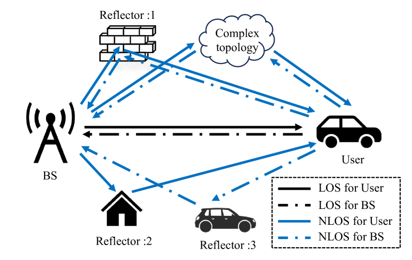
Figure 1: The LOS and NLOS path for the ISAC system.

Motivated by the pursuit of amplifying the sensing gain and elaborating on existing studies related to NLOS challenges, we introduce a novel NOMA-integrated OTFS-ISAC framework tailored for multi-user scenarios, exhibiting potential for deployment within robust, high-velocity mobile networks anchored on UAVs. Within this context, The UAV is regarded as an air BS, where the LOS path between the user and UAV can be guaranteed to attend in the system [26]. After the UAV obtains the user’s position and velocity via the signal echo spread in the LOS channel, the 3D motion prediction topology is implemented to guide the NOMA transmission for multiple users. In addition, the influence of imperfect channel estimation will be evaluated in two NOMA classic problems: max-min fairness (MMF) and maximum sum-rate (SR). The SR problem focuses on increasing the sum rate of the system, whereas the MMF problem ensures fairness between users.

Our novel contributions are explicitly contrasted in Table I and are further summarised as follows:

TABLE I: CONTRASTING THE CONTRIBUTIONS OF THIS WORK TO THE LITERATURE

Contribution	This work	[19]	[15],[18],[21]	[27],[28]	[23],[24]	[29],[30]	[31]
Radar sensing	$\checkmark$	$\checkmark$	$\checkmark$	$\checkmark$	$\checkmark$		$\checkmark$
OTFS	$\checkmark$	$\checkmark$	$\checkmark$			$\checkmark$
NOMA for multiple user	$\checkmark$				$\checkmark$	$\checkmark$
3D motion model	$\checkmark$			$\checkmark$
Multiple path for ISAC system	$\checkmark$	$\checkmark$					$\checkmark$
Robust power allocation	$\checkmark$

• We propose a NOMA-assisted OTFS-ISAC system, where the UAV serves as the air BS to support multiple users. By employing ISAC, the UAV extracts the position and velocity information from the user’s echo signals during communication. On the UAV side, non-orthogonal power allocation is conducted based on the extracted information to achieve a superior data rate.

• Additionally, we examine a three-dimensional motion model, where the distance, velocity, and angle of the user are retrieved from echo signals. The above parameters can only describe the LOS channel between the UAV and the user, hence, the robust power allocation will be investigated with considering the impact of the NLOS channel.

• We derive a closed-form solution to the MMF and SR problem involving non-orthogonal power allocation in OTFS-ISAC systems. Simulation results demonstrate the superiority of our proposed NOMA-assisted OTFS-ISAC system over the OMA-assisted OTFS-ISAC system in terms of MMF and SR.

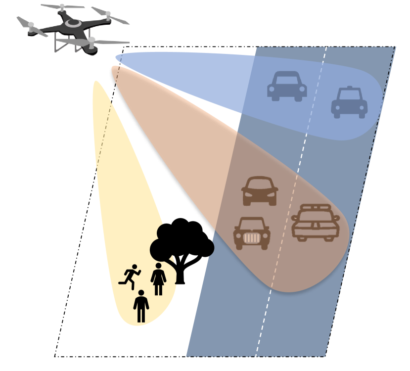
Figure 2: NOMA-assisted OTFS-ISAC networks

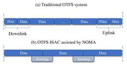
Figure 3: The comparison between the transmission protocol

II OTFS-ISAC system assisted by NOMA

The NOMA-assisted OTFS-ISAC network is shown in Fig. 2, where a UAV supports $G$ clusters and the $g$-th cluster has $P_{g}$ users, where the $g\in\left\{1,2,\dots,G\right\}$. We assume the UAV is equipped with 2 UPAs. One UPA at the UAV transmits the OTFS-ISAC signal to all clusters while the other receives the echo signal from the users. We presume that echo signals do not interact with one another. As shown in the Fig 2, the UAV performs beamforming for the following time slot after analyzing the users’ motion parameters acquired from echoes in the preceding time slot. We assume that users are autonomous and do not block each other during the movement.

The transmission protocol of the traditional OTFS communication system and the NOMA-assisted OTFS-ISAC system are contrasted in Fig. 3 . Specifically, as illustrated in Fig. 3, pilots are required to be transmitted before the data transmission in the conventional OTFS system. Additionally, the CSI obtained in the previous data frame would be outdated for the subsequent frame, resulting in communication performance degradation. By contrast, in a NOMA-assisted OTFS-ISAC system, the UAV can obtain the position and velocity of the users through echoes at no additional cost. The UAV can obtain the OTFS channel by converting the position and velocity information into delay and Doppler information, the user can bypass the step of channel estimation by the UAV’s pre-processing, resulting in pilot-free transmission. In addition, the large-scale fading inferred from the position can guide the power allocation of NOMA, which in turn can improve the data rate of the OTFS-ISAC system.

II-A OTFS-ISAC signal

At the transmitter, we assume that the UAV transmits the OTFS-modulated symbol $x_{p,g}[k,l]$ in the DD domain to the $p$-th user in the $g$-th cluster $U_{p,g}$, where $k=0,1,\cdots,N-1$ and $l=0,1,\cdots,M-1$ are the Doppler and delay indices, respectively. Here, $M$ and $N$ represent the total number of subcarriers and time slots, respectively. The DD-domain signal is then converted to the TF-domain using the inverse symplectic finite Fourier transform (ISFFT), which can be expressed as:

$$X_{p,g}{[n,m]}= \frac{1}{\sqrt{NM}}\sum_{k=0}^{N-1}\sum_{l=0}^{M-1}x_{p,g}[k,l]e^{j2\pi\left(\frac{nk}{N}-\frac{ml}{M}\right)},$$ (1)

where $n=0,1,\cdots,N-1$ and $m=0,1,\cdots,M-1$ are the time and frequency indices in the TF-domain.

Invoking the ideal rectangular transmit pulse $g_{\rm{tx}}(t)$, the time-domain signal $X_{p,g}{[n,m]}$ is converted to the continuous waveform $s_{p,g}(t)$ by the Heisenberg transform, which is expressed as:

$$s^{p}_{g}(t)= \sum_{n=0}^{N-1}\sum_{m=0}^{M-1}X_{p,g}[n,m]g_{\rm{tx}}(t-nT)e^{j2\pi m\Delta f(t-nT)}.$$ (2)

To serve $P_{g}$ users in the $g$-th cluster, the UAV transmits the superimposed signal $s_{g}(t)=\sum_{p=1}^{P_{g}}\omega_{p,g}s_{p,g}(t)$, where $\omega_{p,g}$ denotes the power assigned to the $p$-th user. The transmitted signal to $G$ clusters can be expressed as $\mathbf{s}(t)={\left[s_{1}(t),s_{2}(t),\ldots,s_{G}(t)\right]}^{\text{T}}$. Considering the UPA with a size of $N_{x}\times N_{y}$, the steering vector $\mathbf{a}\left(\theta_{g},\varphi_{g}\right)\in\mathbb{C}^{N_{x}N_{y}\times 1}$ can be defined as:

$$\begin{split}\mathbf{a}\left(\theta_{g},\varphi_{g}\right)=&\frac{1}{\sqrt{N_{x}N_{y}}}\left[1,\ldots,e^{j\pi\sin\theta_{g}\left(n_{x}\sin\varphi_{g}+n_{y}\cos\varphi_{g}\right)}\right.,\\ &\left.\ldots,e^{j\pi\sin\theta_{g}\left(N_{x}\sin\varphi_{g}+N_{y}\cos\varphi_{g}\right)}\right]^{\text{T}},\end{split}$$ (3)

where the $\theta_{g}$ and $\varphi_{g}$ are the azimuth and elevation of the $g$-the cluster, respectively. Additionally, $n_{x}=1,2,\dots,N_{x}$ and $n_{y}=1,2,\dots,N_{y}$ are the indices of the transmit antenna. Defining $\mathbf{A}={\left[\mathbf{a}\left(\theta_{1},\varphi_{1}\right),\dots,\mathbf{a}\left(\theta_{G},\varphi_{G}\right)\right]}$, the transmitted signal can be formulated as:

$${\bar{\mathbf{s}}}(t)= \mathbf{A}\mathbf{s}(t).$$ (4)

II-B Radar Sensing Process

The UAV receives the echo signal via the radar channel $\mathbf{H}_{p,g}(t,\tau)$, which can be expressed as:

$$\begin{split}&\mathbf{H}_{p,g}(t,\tau)=\beta_{p,g}\mathbf{b}\left(\theta_{p,g},\varphi_{p,g}\right)\mathbf{b}^{\mathrm{H}}\left(\theta_{p,g},\varphi_{p,g}\right)\delta\left(t-\tau_{p,g}\right)\times\\ &e^{j2\pi\nu_{p,g}t}+\sum_{i=1}^{N_{p,g}}\hat{\beta}_{p,g}^{\text{R},i}\mathbf{b}\left(\hat{\theta}_{p,g}^{\text{R},i},\hat{\varphi}_{p,g}^{\text{R},i}\right)\mathbf{b}^{\mathrm{H}}\left(\hat{\theta}_{p,g}^{\text{R},i},\hat{\varphi}_{p,g}^{\text{R},i}\right)\delta\left(t-\hat{\tau}_{p,g}^{\text{R},i}\right)e^{j2\pi\hat{\nu}_{p,g}^{\text{R},i}t}.\end{split}$$ (5)

where the $\beta_{p,g}$, $\tau_{p,g}$ and $\nu_{p,g}$ respectively represent the reflection coefficient, delay and the Doppler offset of the LOS channel with the direction $\left(\theta_{p,g},\varphi_{p,g}\right)$ between the $p$-th user in the $g$-th cluster and the UAV. The $\beta_{p,g}^{\text{R},i}$, $\tau_{p,g}^{\text{R},i}$ and $\nu_{p,g}^{\text{R},i}$ represent the reflection coefficient, delay and the Doppler offset of the $i$-th radar NLOS path with the direction $\left(\theta_{p,g}^{\text{R},i},\varphi_{p,g}^{\text{R},i}\right)$.

In Eq.(5) $\mathbf{b}\left(\theta_{p,g},\varphi_{p,g}\right)$ is the receive steering vector, which can be expressed as:

$$\begin{split}\mathbf{b}\left(\theta_{p,g},\varphi_{p,g}\right)=&\frac{1}{\sqrt{N_{x}N_{y}}}\left[1,\ldots,e^{j\pi\sin\theta_{p,g}\left(n_{x}\sin\varphi_{p,g}+n_{y}\cos\varphi_{p,g}\right)}\right.,\\ &\left.\ldots,e^{j\pi\sin\theta_{p,g}\left(N_{x}\sin\varphi_{p,g}+N_{y}\cos\varphi_{p,g}\right)}\right]^{T}.\end{split}$$ (6)

The $\mathbf{b}\left(\hat{\theta}_{p,g}^{\text{R},i},\hat{\varphi}_{p,g}^{\text{R},i}\right)$ will be obtained by replacing the $\theta_{p,g}$ and $\varphi_{p,g}$ in $\mathbf{b}\left(\theta_{p,g},\varphi_{p,g}\right)$ with $\hat{\theta}_{p,g}^{\text{R},i}$ and $\hat{\varphi}_{p,g}^{\text{R},i}$.

Furthermore, the echo signal of $U_{p,g}$ can be formulated as:

$$\begin{split}&\mathbf{r}_{p,g}(t)=\beta_{p,g}\mathbf{b}\left(\theta_{p,g},\varphi_{p,g}\right)\mathbf{b}^{\mathrm{H}}\left(\theta_{p,g},\varphi_{p,g}\right)\mathbf{a}\left(\theta_{g},\varphi_{g}\right)\times\\ &s_{g}(t-\tau_{p,g})e^{j2\pi\nu_{p,g}t}+\sum_{i=1}^{N_{p,g}}\hat{\beta}_{p,g}^{\text{R},i}\mathbf{b}\left(\hat{\theta}_{p,g}^{\text{R},i},\hat{\varphi}_{p,g}^{\text{R},i}\right)\mathbf{b}^{\mathrm{H}}\left(\hat{\theta}_{p,g}^{\text{R},i},\hat{\varphi}_{p,g}^{\text{R},i}\right)\\ &\times\mathbf{a}\left(\theta_{g},\varphi_{g}\right)s_{g}\left(t-\hat{\tau}_{p,g}^{\text{R},i}\right)e^{j2\pi\hat{\nu}_{p,g}^{\text{R},i}t}+\mathbf{z}(t),\end{split}$$ (7)

where the $\mathbf{z}(t)$ is the white Gaussian noise.

To facilitate communication, the channel parameters can be obtained by following steps. First, the angle $\left(\theta_{p,g},\varphi_{p,g}\right)$ and $\left(\hat{\theta}_{p,g}^{\text{R},i},\hat{\varphi}_{p,g}^{\text{R},i}\right)$ can be estimated by using a mature method called MUSIC [32], which has great efficiency and high resolution. Then, the echo signal without angle information can be expressed as:

$$\begin{split}\bar{r}_{p,g}(t)=\beta_{p,g}s_{g}(t-\tau_{p,g})e^{j2\pi\nu_{p,g}t}+\sum_{i=1}^{N_{p,g}}\hat{\beta}_{p,g}^{\text{R},i}s_{g}(t-\hat{\tau}_{p,g}^{\text{R},i})e^{j2\pi\hat{\nu}_{p,g}^{\text{R},i}t}.\end{split}$$ (8)

Second, the UAV performs MF on the echo signal to obtain $\tau_{p,g}$, $\nu_{p,g}$, $\hat{\tau}_{p,g}^{\text{R},i}$ and $\hat{\nu}_{p,g}^{\text{R},i}$. The correlated value function $\jmath(\tau,\nu)$ can be represented as follows:

$$\jmath(\tau,\nu)=\int_{0}^{\Delta T}\bar{r}_{p,g}(t){{s}_{g}}^{*}(t-\tau)e^{-j2\pi\nu t}\mathrm{~{}d}t,$$ (9)

where $\Delta T$ represents the frame time duration, and $*$ represents the conjugate operator. Although, both the radar’s LOS and NLOS channel information can be obtained by the radar sensing process, only the LOS channel of radar is highly correlated to the LOS channel of communication, which can be applied in the communication pre-processing. The NLOS channel sensed by the radar is different from the NLOS channel in the communication. But, the NLOS path sensed by the radar can describe the complexity of the environment [33], where we define $e_{p,g}$ to represent the strength of the NLOS channel in the environment:

$$e_{p,g}=\frac{\sum_{i=1}^{N_{p,g}}\left(\hat{\beta}_{p,g}^{\text{R},i}\right)^{2}}{\left(\beta_{p,g}\right)^{2}}.$$ (10)

The estimated of $e_{p,g}$ can be obtained by the function $\jmath(\tau,\nu)$:

$$\hat{e}_{p,g}=\frac{\sum_{i=1}^{N_{p,g}}\left(\jmath(\hat{\tau}_{p,q}^{\text{R},i},\hat{\nu}_{p,q}^{\text{R},i})\right)^{2}}{\left(\jmath(\tau_{p,q},\nu_{p,q})\right)^{2}},$$ (11)

which will be considered in the following NOMA power allocation.

II-C Communication Process

The communication channel is different from the radar channel, which is consisted by multiple paths from UAV to the user, with the LOS path predominating. The communication channel between the $p$-th user in the $g$-th cluster and the UAV can be expressed as:

$${\mathbf{\bar{H}}}_{p,g}\left(t,\tau\right)=h_{p,g}\mathbf{b}^{\text{H}}\left(\theta_{p,g},\varphi_{p,g}\right)\delta\left(t-\frac{\tau_{p,g}}{2}\right)e^{j2\pi\nu_{p,g}t}$$

$$+\sum_{i=1}^{N_{p,g}}\hat{h}_{p,q}^{\text{C},i}\mathbf{b}^{\text{H}}\left(\hat{\theta}_{p,g}^{\text{C},i},\hat{\varphi}_{p,g}^{\text{C},i}\right)\delta\left(t-\hat{\tau}_{p,q}^{\text{C},i}\right)e^{j2\pi\hat{\nu}_{p,q}^{\text{C},i}t}.$$ (12)

where $h_{p,g}$ and $\hat{h}_{p,q}^{\text{C},i}$ represent the large scale loss of the LOS and NLOS, respectively. Additionally, $\left(\hat{\theta}_{p,g}^{\text{C},i},\hat{\varphi}_{p,g}^{\text{C},i}\right)$ represents the receive direction of $i$-th NLOS, whereas $\hat{\tau}_{p,q}^{\text{C},i}$ and $\hat{\nu}_{p,q}^{\text{C},i}$ represent the $i$-th NLOS’s delay and Doppler offset, respectively. Consequently, the received signal is expressed as:

$$\begin{split}y_{p,g}(t)={\mathbf{\bar{H}}}_{p,g}\left(t,\tau\right)\mathbf{a}\left(\theta_{g},\varphi_{g}\right)s_{p,g}(t).\end{split}$$ (13)

As soon as $y_{g,p}(t)$ is received, Wigner transform is performed to translate the time-domain signal to the TF domain.

$$Y_{p,g}[n,m]= \int_{t^{\prime}}g_{\text{rx}}\left(t^{\prime}-t\right)y_{p,g}\left(t^{\prime}\right)$$

$$\times e^{-j2\pi f\left(t^{\prime}-t\right)}dt^{\prime}|_{t=nT,f=m\Delta f},$$ (14)

where $g_{\text{rx}}\left(t\right)$ is the ideal rectangular pulse. Then, the Symplectic finite Fourier transform (SFFT) is applied to the discrete signal $Y_{p}[n,m]$ to obtain the information $y_{p}[k,l]$ in the DD domain.

$$y_{p,g}[k,l]=\frac{1}{\sqrt{NM}}\sum_{n=0}^{N-1}\sum_{m=0}^{M-1}{Y_{p,g}}[n,m]e^{-j2\pi\left(\frac{nk}{N}-\frac{ml}{M}\right)}.$$ (15)

II-D Three-dimensional motion topology

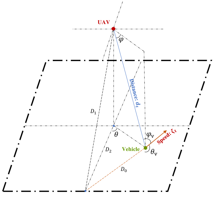
Figure 4: The 3-D user movement model

In our proposed NOMA-assisted OTFS-ISAC system, the UAV assists the OTFS-ISAC signal transmission by estimating the user’s position in the next time slot. Hence, a 3D motion model is introduced to improve estimation precision of the user’s position in the subsequent time slot. Fig. 4 depicts a schematic of topological 3D motion, where the UAV estimates relavant parameters of the users on the ground. We assume that the angle of the velocity $\theta_{v}$ has been derived from the user position in the previous time slot. At the time slot $t$, the distance between the user and the UAV is $d_{t}$, while the azimuth and elevation angle are $\theta$ and $\varphi$, respectively. The distance $d_{t}$ can be calculated using the delay $\tau_{t}$ and the velocity of light $c$:

$$\begin{split}d_{t}=\frac{c\tau_{t}}{2}.\end{split}$$ (16)

According to the geometric relationship, the angle $\varphi_{v}$ between the line connecting UAV and the user and the speed is given by

$$\begin{split}\varphi_{v}=\pi-\arccos{\left(\frac{{d_{t}}^{2}+{\left(D_{0}\right)}^{2}-\left(D_{1}\right)^{2}}{2d_{t}D_{0}}\right)},\end{split}$$ (17)

where we have:

$$\begin{split}D_{0}=&\frac{d_{t}\sin\theta\cos\varphi}{\sin\left(\pi-\theta_{v}\right)},\\ D_{1}=&\sqrt{\left(d_{t}\sin\varphi\right)^{2}+\left(D_{2}\right)^{2}},\\ D_{2}=&\frac{\sin\left(\pi-\theta_{v}\right)d_{t}\cos\varphi}{\sin\left(\theta_{v}-\theta\right)},\end{split}$$ (18)

where $D_{0}$, $D_{1}$ and $D_{2}$ represent the actual line segments that have been labelled in Fig. 4. Furthermore, the user velocity $\zeta_{t}$ can be derived from $\varphi_{v}$ and $\nu_{t}$ in the time slot $t$:

$$\begin{split}\zeta_{t}=\frac{c\nu_{t}}{\cos\varphi_{v}f_{c}},\end{split}$$ (19)

where $f_{c}$ is the carrier frequency. According to the 3D model, we may deduce the distance $d_{t+1}$ between the UAV and the user at the next time slot $t+1$:

$$\begin{split}d_{t+1}=\sqrt{{\left(d_{t}+\zeta_{t}T_{\text{otfs}}-d_{t}\sin\phi\right)}^{2}+{\left(d_{t}\sin\phi\right)}^{2}}.\end{split}$$ (20)

$$\begin{split}\phi=\arccos{\left(\frac{{D_{0}}^{2}+{\left(D_{1}\right)}^{2}-\left(d_{t_{0}}\right)^{2}}{2D_{0}D_{1}}\right)}.\end{split}$$ (21)

The $T_{\text{otfs}}$ represents the estimation interval for each place.

III Power allocation for the perfect and imperfect channel

In this section, we present a power allocation algorithm for NOMA under perfect and imperfect channel assumptions in the context of two classic NOMA problems, namely MMF and SR. The LOS path information is inferred from users’ position and speed, which can be obtained via our proposed 3D motion model. The perfect channel assumption considers only the LOS path, whereas the imperfect channel assumption accounts for both LOS and NLOS paths. Classic NOMA strategies often employ user-pairing to maintain tractable complexity, as highlighted in [34, 35]. Moreover, methodologies for multi-user pairing have received substantial attention, as delineated in [36, 37]. In the context of this paper, and without compromising generality, we delve into power distribution post-user-pairing, specifically for a dual-user setup. Our proposed framework exhibits scalability for accommodating a broader user base by employing existing pairing techniques. The power allocated to User 1 (U1) and User 2 (U2) is denoted as $\omega_{1}$ and $\omega_{2}$, respectively. The achievable rates achieved by U1 and U2 with successive interference cancellation (SIC) are denoted as $R_{1}$ and $R_{2}$, respectively.

III-A Perfect Channel

Assuming perfect channel conditions, the communication channel is modeled as a point-to-point system dominated by LOS transmission, ignoring NLOS effects [38]. The large-scale fading factor, $h_{p}$, represents the path loss between the UAV and the $p$-th user for any given cluster, where $\left|h_{1}\right|^{2}\leq\left|h_{2}\right|^{2}$. Additionally, the distance between the UAV and $p$-th user, denoted by $d_{p}$, is defined. The angle-dependent differences in $h_{p}$ for U1 and U2, which are illuminated by a single beam, can be neglected. As a result, the expression for $h_{p}$ for U1 and U2 can be defined as:

$$\begin{split}h_{p}=\frac{G_{\text{T}}G_{\text{R}}\lambda^{2}}{(4\pi)^{2}{d_{p}}^{2}},\end{split}$$ (22)

where $G_{\text{T}}$ and $G_{\text{R}}$ represent the transmit gain and receive gain, respectively, and $\lambda$ denotes the wavelength of electromagnetic waves. The achievable rate of U1 and U2 using NOMA is formulated as follows:

$$\begin{split}R_{1}=\log{2}\left(1+\frac{\omega_{1}\left|h_{1}\right|^{2}}{\omega_{2}\left|h_{1}\right|^{2}+n_{0}}\right),\end{split}$$ (23)

and

$$\begin{split}R_{2}=\log{2}\left(1+\frac{\omega_{2}\left|h_{2}\right|^{2}}{n_{0}}\right).\end{split}$$ (24)

III-A1 Maximin Fairness

In order to ensure fairness among different users, the MMF problem is introduced. Mathematically, this problem can be formulated as

$$(P1):\mathop{\max\min}\limits_{\omega_{1},\omega_{2}}\quad \left\{R_{1},R_{2}\right\}$$ (25)

$$s.t.\quad \omega_{1}+\omega_{2}\leq P_{\text{t}},$$ (25a)

The aim of this problem is to maximize the rate of the minimum rate user, thus promoting fairness among users. The optimal power allocation for U2 in the MMF problem can be obtained as $\omega_{2,\text{MMF}}^{*}=\frac{-\left(\left|h_{1}\right|^{2}n_{0}+\left|h_{2}\right|^{2}n_{0}\right)+\sqrt{\left(\left|h_{1}\right|^{2}n_{0}+\left|h_{2}\right|^{2}n_{0}\right)^{2}+4P\left|h_{1}\right|^{4}\left|h_{2}\right|^{2}n_{0}}}{2\left|h_{1}\right|^{2}\left|h_{2}\right|^{2}}$. The value of $\omega_{1,\text{MMF}}$ is then determined as $\omega_{1,\text{MMF}}^{*}=P_{\text{t}}-\omega_{2,\text{MMF}}^{*}$. The proof could be found in [34].

III-A2 Sum-Rate

The primary goal of SR is to optimize the rate while adhering to the constraints of the quality of service. This optimization problem is expressed as (P2), where the objective is to maximize the sum of R1 and R2:

$$(P2):\mathop{\max}\limits_{\omega_{1},\omega_{2}}\quad R_{1}+R_{2},$$ (26)

s.t $$R_{1}\geq R_{1,\text{min}},$$ (26a)

$$R_{2}\geq R_{2,\text{min}},$$ (26b)

$$\omega_{1}+\omega_{2}\leq P_{\text{t}}.$$ (26c)

The optimization problem above is subject to the constraints 26(a)-26(c), which require $R_{1}$ and $R_{2}$ to be higher than or equal to their respective minimum required rates, and the total power transmitted by U1 and U2 to be less than or equal to $P_{t}$. In this problem, $R_{1,\text{min}}$ and $R_{2,\text{min}}$ represent the minimum required rates for U1 and U2, respectively. By fully utilizing the transmit power, we set $\omega_{1}=P_{\text{t}}-\omega_{2}$. The optimization function can be expressed $f_{\text{SR}}(\omega_{2})=R_{1}+R_{2}$, where the derivative function $f’_{\text{SR}}(\omega_{2})$ is expressed as

$${f’_{\text{SR}}}(\omega_{2})=\frac{\left(\left|h_{2}\right|^{2}-\left|h_{1}\right|^{2}\right)n_{0}^{2}}{\left(\omega_{2}\left|h_{2}\right|^{2}+n_{0}\right)\left(\omega_{2}\left|h_{1}\right|^{2}+n_{0}\right)n_{0}}.$$ (27)

Under the condition $\left|h_{1}\right|^{2}\leq\left|h_{2}\right|^{2}$, $f^{\prime}_{1}(\omega_{2})$ is always positive, which indicates that the optimal solution is obtained at the upper bound of $\omega_{2}$. In order to meet the constraints 26(a) and 26(b), the upper and lower bounds of $\omega_{2}$ are calculated as $\frac{P_{\text{t}}\left|h_{1}\right|^{2}-\left(2^{R_{1,\text{min}}}-1\right)n_{0}}{\left(2^{R_{1,\text{min}}}-1\right)\left|h_{1}\right|^{2}+\left|h_{1}\right|^{2}}$ and $\frac{\left(2^{R_{2,\text{min}}}-1\right)n_{0}}{\left|h_{2}\right|^{2}}$, respectively. Therefore, the optimal power allocation for U2 in the SR problem is given by $\omega_{2,\text{SR}}^{*}=\frac{P_{\text{t}}\left|h_{1}\right|^{2}-\left(2^{R_{1,\text{min}}}-1\right)n_{0}}{\left(2^{R_{1,\text{min}}}-1\right)\left|h_{1}\right|^{2}+\left|h_{1}\right|^{2}}$, and the corresponding optimal power to be allocated to U1 is $\omega_{1,\text{SR}}^{*}=P_{\text{t}}=\omega_{2,\text{SR}}^{*}$.

III-B Imperfect Channel

In practical scenarios, the identification of the LOS channel from the echo signal is possible for the OTFS-ISAC system, while the NLOS channel cannot be perfectly sensed, resulting in a received signal that is a superposition of the known LOS and unknown NLOS signals. To demonstrate this phenomenon, the real channel fading $\bar{h}_{p}$ can be expressed as the sum of the true LOS channel $h_{p}$ and an estimated NLOS channel $\hat{h}_{p}$, given by:

$$\begin{split}\bar{h}_{p}=h_{p}+\hat{h}_{p},\end{split}$$ (28)

where $\hat{h}_{p}\sim\mathcal{CN}\left(0,e_{p}{|h_{p}|}^{2}\right)$ represents the NLOS channel, and $e_{p}$ denotes the complexity of the environment obtained by the radar sensing. A larger value of $e_{p}$ signifies the presence of more reflectors with higher reflection coefficients in the environment.

We introduce the notations $\bar{R}_{1}$ and $\bar{R}_{2}$ to represent the transmission achievable rates of users U1 and U2, respectively, when operating in an imperfect channel. The lower bound of $\bar{R}_{1}$ and $\bar{R}_{2}$ is established by considering the NLOS channel as interference. For user U1, the power of user U2, denoted by $E\left\{\omega_{2}\left({|h_{1}|}^{2}+{|\hat{h}_{1}|}^{2}\right)\right\}=\omega_{2}\left(\left|h_{1}\right|^{2}+e_{1}\left|h_{1}\right|^{2}\right)$, along with the NLOS component of user U1, denoted by $E\left\{\omega_{1}{|\hat{h}_{1}|}^{2}\right\}=\omega_{1}e_{1}\left|h_{1}\right|^{2}$, are treated as noise. For user U2, the interference caused by the LOS component power of user U1 is removed through Successive Interference Cancellation (SIC), but the NLOS component power of user U1 still remains. Therefore, the NLOS component power of user U1, denoted by $E\left\{\omega_{1}{|\hat{h}_{2}|}^{2}\right\}=\omega_{1}e_{2}\left|h_{2}\right|^{2}$ , and user U2, denoted by $E\left\{\omega_{2}{|\hat{h}_{2}|}^{2}\right\}=\omega_{2}e_{2}\left|h_{2}\right|^{2}$, are considered as noise for user U2. The lower bounds of the transmission achievable rates for U1 and U2 are expressed respectively as:

$$\begin{split}\bar{R}_{1}^{\text{L}}=\log_{2}\left(1+\frac{\omega_{1}\left|h_{1}\right|^{2}}{\omega_{2}\left(\left|h_{1}\right|^{2}+e_{1}\left|h_{1}\right|^{2}\right)+\omega_{1}e_{1}\left|h_{1}\right|^{2}+n_{0}}\right),\end{split}$$ (29)

and

$$\begin{split}\bar{R}_{2}^{\text{L}}=\log_{2}\left(1+\frac{\omega_{2}\left|h_{2}\right|^{2}}{\omega_{1}e_{2}\left|h_{2}\right|^{2}+\omega_{2}e_{2}\left|h_{2}\right|^{2}+n_{0}}\right).\end{split}$$ (30)

Conversely, the upper bounds of $\bar{R}_{1}$ and $\bar{R}_{2}$ are obtained when the NLOS is leveraged for communication. The extra power to boost the rate is represented by $\omega_{1}e_{1}\left|h_{1}\right|^{2}$ and $\omega_{2}e_{2}\left|h_{2}\right|^{2}$ for users U1 and U2, respectively. The upper bounds of the transmission achievable rates can be expressed respectively as:

$$\begin{split}\bar{R}_{1}^{\text{U}}=\log_{2}\left(1+\frac{\omega_{1}\left(\left|h_{1}\right|^{2}+e_{1}\left|h_{1}\right|^{2}\right)}{\omega_{2}\left(\left|h_{1}\right|^{2}+e_{1}\left|h_{1}\right|^{2}\right)+n_{0}}\right),\end{split}$$ (31)

and

$$\begin{split}\bar{R}_{2}^{\text{U}}=\log_{2}\left(1+\frac{\omega_{2}\left(\left|h_{2}\right|^{2}+e_{2}\left|h_{2}\right|^{2}\right)}{\omega_{1}e_{2}\left|h_{2}\right|^{2}+n_{0}}\right).\end{split}$$ (32)

III-B1 MMF

In the presence of an imperfect channel, the problem of optimizing the max-min fairness (MMF) becomes a constrained optimization problem, denoted by (P3), as:

$$\text{(P3)}:\mathop{\max\min}\limits_{\omega_{1},\omega_{2}}\quad \left\{\bar{R}_{1},\bar{R}_{2}\right\},$$ (33)

$$s.t.\quad \omega_{1}+\omega_{2}\leq P_{\text{t}},$$ (33a)

The objective function of (P3) is to maximize the minimum achievable rate, denoted by ${\bar{R}_{1},\bar{R}_{2}}$. The constraint is that the sum of the power allocations for users U1 and U2 should not exceed the total transmit power $P_{\text{t}}$. When the lower bound performance of MMF is optimized, it is assumed that the channels for both users are highly correlated since U1 and U2 are in the same beam, i.e., $e_{1}=e_{2}=e$. In this case, the power allocation for user U2 can be expressed as $\omega_{2,\text{MMF}}^{{\text{L}},0}=\sqrt{P_{\text{t}}^{2}e^{2}+P_{\text{t}}^{2}e}-P_{\text{t}}e$ when the achievable rates for both users are equal, i.e., $\bar{R}_{1}^{\text{L}}=\bar{R}_{2}^{\text{L}}$. If $\omega_{2}\geq\omega_{2,\text{MMF}}^{\text{L},0}$, the objective function of (P3) becomes ${\bar{R}_{1}^{\text{L}}}$, which increases as $\omega_{2}$ decreases. On the other hand, if $\omega_{2}\leq\omega_{2,\text{MMF}}^{{\text{L}},0}$, the objective function of (P3) becomes ${\bar{R}_{2}^{\text{L}}}$, which increases as $\omega_{2}$ increases. Therefore, the optimal power allocation for users U1 and U2 in the lower bound of MMF is $\omega_{2,\text{MMF}}^{\text{L},*}=\omega_{2,\text{MMF}}^{\text{L},0}$ and $\omega_{1,\text{MMF}}^{\text{L},*}=P_{\text{t}}-\omega_{2,\text{MMF}}^{\text{L},0}$, respectively. The upper bound performance of the MMF optimization problem (P3) is investigated by assuming that the achievable rates for both users are equal, denoted by $\bar{R}_{1}^{\text{U}}=\bar{R}_{2}^{\text{U}}$. The optimal power allocation for user U2 in the upper bound of MMF is then obtained as $\omega_{2,\text{MMF}}^{\text{U},*}=\sqrt{1+e}-1$, and the optimal power allocation for user U1 is obtained as $\omega_{1,\text{MMF}}^{\text{U},*}=P_{\text{t}}-\omega_{2,\text{MMF}}^{\text{U},*}$, using a similar derivation as for the lower bound.

III-B2 Sum-Rate

The SR optimization under imperfect channel can be formulated as:

$$(P4):\mathop{\max}\limits_{\omega_{1},\omega_{2}}\quad \bar{R}_{1}+\bar{R}_{2},$$ (34)

s.t $$\bar{R}_{1}\geq R_{1,\text{min}},$$ (34a)

$$\bar{R}_{2}\geq R_{2,\text{min}},$$ (34b)

$$\omega_{1}+\omega_{2}\leq P_{\text{t}}.$$ (34c)

The objective function of (P4) is to maximize the sum of achievable rates for users U1 and U2, denoted by $\bar{R}_{1}+\bar{R}_{2}$. The constraints of (P4) ensure that the achievable rates for both users are greater than or equal to a minimum rate requirement, denoted by $R_{1,\text{min}}$ and $R_{2,\text{min}}$, respectively. In addition, the total power allocated to users U1 and U2 should not exceed the total transmit power, denoted by $P_{\text{t}}$.

To investigate the lower bound performance of SR in (P4), we assume that the achievable rates for both users are equal to the lower bound of achievable rates, denoted by $\bar{R}_{1}^{\text{L}}$ and $\bar{R}_{2}^{\text{L}}$, respectively. The object function of (P4) for the lower bound can be expressed as ${f^{\text{L}}_{\text{SR}}}\left(\omega_{2}\right)=\bar{R}_{1}^{\text{L}}+\bar{R}_{2}^{\text{L}}$, where the power allocation for user U1 is $\omega_{1}=P_{\text{t}}-\omega_{2}$. It is guaranteed that the corresponding derivative function ${f^{\text{L}}_{\text{SR}}}^{\prime}\left(\omega_{2}\right)>0$ when $\omega_{2}\in[0,P_{\text{t}}]$. The optimal power allocation for user U2 in the lower bound of SR, denoted by $\omega_{2,\text{SR}}^{\text{L},*}$, can be obtained by finding the upper bound of $\omega_{2}$ that satisfies the constraints in (34a) and (34b). The optimal power allocation for user U2 is then expressed as $\omega_{2,\text{SR}}^{\text{L},*}=\frac{P_{\text{t}}(1+e)+n_{0}/|h_{1}|^{2}}{2^{R_{1,\text{min}}}}-P_{\text{t}}e-n_{0}/|h_{1}|^{2}$, and the corresponding optimal power allocation for user U1 is $\omega_{1,\text{SR}}^{\text{L},*}=P_{\text{t}}-\omega_{2,\text{SR}}^{\text{L},*}$.

Then, in order to analyse the upper bound performance of the SR problem, denoted by (P4), we set $\bar{R}_{1}=\bar{R}_{1}^{\text{U}},~{}\bar{R}_{2}=\bar{R}_{2}^{\text{U}}$ in P(4). Using the power allocation $\omega_{1}=P_{\text{t}}-\omega_{2}$, the object function of (P4) is defined as $f_{\text{SR}}^{\text{U}}\left(\omega_{2}\right)=\bar{R}_{1}^{\text{U}}+\bar{R}_{2}^{\text{U}}$, which is further expressed as:

$$\begin{split}f_{\text{SR}}^{\text{U}}\left(\omega_{2}\right)=&\log_{2}\left({\frac{P_{\text{t}}(1+e)+\frac{n_{0}}{|h_{1}|^{2}}}{P_{\text{t}}e+\omega_{2}+\frac{n_{0}}{|h_{1}|^{2}}}}\right)\\ +&\log_{2}\left({\frac{P_{\text{t}}(e+2)-\omega_{2}+\frac{n_{0}}{|h_{2}|^{2}}}{P_{\text{t}}e+\frac{n_{0}}{|h_{2}|^{2}}}}\right)\end{split}$$ (35)

where the terms $\frac{n_{0}}{|h_{1}|^{2}}$ and $\frac{n_{0}}{|h_{2}|^{2}}$ can be ignored as they are very small compared to the others. Hence, the derivative function ${f_{\text{SR}}^{\text{U}}}^{{}^{\prime}}\left(\omega_{2}\right)$ can be simply expressed:

$$\begin{split}{f_{\text{SR}}^{\text{U}}}^{{}^{\prime}}\left(\omega_{2}\right)=\frac{{\omega_{2}}^{2}+2P_{\text{t}}e\omega_{2}-P_{\text{t}}^{2}}{\ln{2}\left(P_{\text{t}}e+\omega_{2}\right)\left(\omega_{2}P_{\text{t}}-\omega_{2}^{2}\right)}.\end{split}$$ (36)

Observe from Eq. (36), the denominator of ${f_{\text{SR}}^{\text{U}}}^{{}^{\prime}}\left(\omega_{2}\right)$ is positive when $0\leq\omega_{2}\leq P_{\text{t}}$. Furthermore, by setting the numerator to 0, the solution for the power allocation of user U2 can be obtained as $\omega_{2,\text{SR}}^{\text{U},0}=\sqrt{e^{2}P^{2}_{\text{t}}+P_{\text{t}}^{2}}-eP_{\text{t}}$. As a result, the function $f_{2}\left(\omega_{2}\right)$ decreases as $\omega_{2}$ increases in the interval $\left(0,\omega_{2,\text{SR}}^{\text{U},0}\right)$ and increases as $\omega_{2}$ increases in the interval $\left(\omega_{2,\text{SR}}^{\text{U},0},P_{\text{t}}\right)$. Therefore, the optimal power allocation for user U2 in the upper bound of the SR problem is $\omega_{2,\text{SR}}^{\text{U},*}=\omega_{2,\text{SR}}^{\text{U},0}$ and the corresponding optimal power allocation for U1 is $\omega_{1,\text{SR}}^{\text{U},*}=P_{\text{t}}-\omega_{2,\text{SR}}^{\text{U},*}$.

IV Numerical Results

In this section, we provide the simulation results for our proposed NOMA-assisted OTFS-ISAC network with the aid of the proposed 3D motion prediction topology. Specifically, we evaluated the MMR and SR performance under perfect and imperfect channel conditions. The simulation parameters are summarized in table II.

TABLE II: Simulation Parameters

Parameter	Value
Carrier frequency (GHz) $f_{c}$	5
OTFS frame size $[M,N]$	[1024,1024]
OTFS symbol duration (ms) $\Delta T$	4.4
Transmit and receive gain (dB) $G_{\text{T}}$ and $G_{\text{R}}$	0
UE speed (Kmph) $v$	[30-60]
Guard frame size	[30,60]
The distance of U1 and U2 (m) $[d_{1},d_{2}]$	[7,15]
Channel estimation error $e$	[0-0.1]

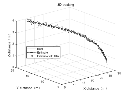
Figure 5: The 3D motion topology estimation.

The performance of a 3D motion topological prediction system is demonstrated in Fig. 5, where the system considers a user’s movement along a curve with time-varying speed $v\in[9,13]~{}\text{m/s}$. The solid line represents the user’s actual movement, while the estimated position is illustrated by the dashed line. A low-pass filter with the method of moveing average is employed to reduce the effect of the radar resolution-induced jitter on the user’s continuous movement, thereby enhancing the accuracy of the position estimation. The proposed 3D motion topological approach successfully recovers the user’s actual position, encompassing both azimuth and elevation information, with an estimation error of approximately 2%, which fulfills the required accuracy level for user position tracking.

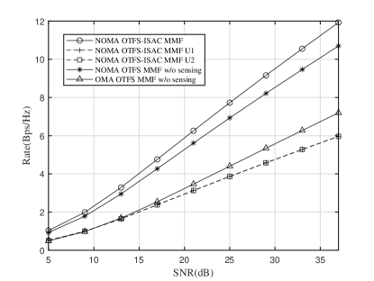
Figure 6: The comparison between different systems in the MMF problem over the perfect channel.

Fig. 6 depicts the achievable rate performance of MMF, assuming perfect channel conditions. The performance of three transmission protocols, namely NOMA-assisted OTFS-ISAC, NOMA-assisted OTFS without sensing, and OMA-assisted OTFS without sensing, are compared under varying values of SNR. Our proposed system outperforms the other systems, as evidenced by its highest achievable rate. The NOMA-assisted version, which enables the spectrum to be shared among different users, yields higher spectral efficiency. The sensing can reduce the pilot overhead, which result in more information can be transmitted in the DD-domain. The objective function of (P1) ensures fairness between U1 and U2, resulting in both users having a rate that is half of the overall rate under different SNR values.

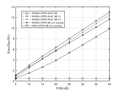
Figure 7: The comparison between different systems in the SR problem over the perfect channel.

Fig. 7 presents the performance of the SR problem in the perfect channel scenario. The proposed NOMA-assisted OTFS-ISAC system, leveraging the benefits of both NOMA and sensing, achieves the highest rate compared to other techniques, consistent with the conclusion of the MMF problem, as depicted in Fig.6. However, the MMF problem fairly satisfies information transmission for multiple users, the SR problem focus demonstrating the overall performance of the ISAC system, whihc aims to maximize the sum rate. Specifically, the system prioritizes increasing the rate of user U2 with the superior channel, while satisfying the minimum rate requirement of user U1 (0.5Bps/Hz). The data rate of user U2 increases with the SNR, surpassing that of user U1.

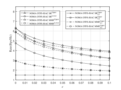
Figure 8: The upper bound and lower bound performance of MMF and SR over the imperfect channel.

To demonstrate the impact of imperfect channel conditions on the system, we depict the extremities—both upper and lower—of MMF and SR against channel estimation inaccuracies, denoted as $e\in[0,0.1]$, in Fig. 8, which is consistent with the range of parameter assumptions for the Rice channel. The upper boundary is derived by interpreting the NLOS power as a distinct gain, whereas the lower demarcation perceives it as interference. Notably, even when the NLOS power is viewed as an isolated gain for the upper threshold, it concurrently introduces interference for the alternative user within the system. This intrinsic relationship is described by the equations Eq. (31) and Eq. (32). As $e$ increases from $0$ to $0.1$, the MMF and SR rates manifest a pronounced deterioration. A diminutive $e$ corresponds to closely spaced upper and lower thresholds for both SR and MMF rates. In scenarios devoid of NLOS (where $e=0$), these thresholds converge. The ascent of $e$ instigates a more pronounced descent in the lower threshold relative to its upper counterpart.Regarding the SR upper boundary, user U1 consistently registers a rate of 1.5 Bps/Hz, sustaining the baseline rate threshold with growing $e$. Conversely, the rate for user U2 exhibits a decrement with the escalation in $e$. Within the MMF upper bound, the rates of users U1 and U2 are equal to ensure fairness. These observations validate the precision of our antecedent NOMA-integrated OTFS-ISAC power distribution approach for both SR and MMF, particularly when accommodating imprecise channel conditions.

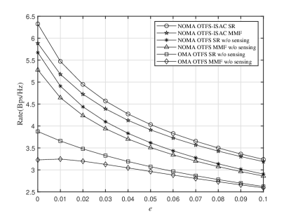
Figure 9: The comparison between different system in MMF and SR problem over the imperfect channel.

Fig.9 presents the evaluation of the proposed system’s superiority over other counterparts without sensing under imperfect channel estimation. The results indicate that the NOMA-assisted OTFS-ISAC system outperforms the benchmark by leveraging the benefits of NOMA and sensing, as discussed in Fig.6. To ensure fairness in the MMF problem, more power is allocated to U1, despite having a worse channel. It is observed that the system’s rate considering the SR is higher than that considering the MMF, as $e$ increases from 0 to 0.1.

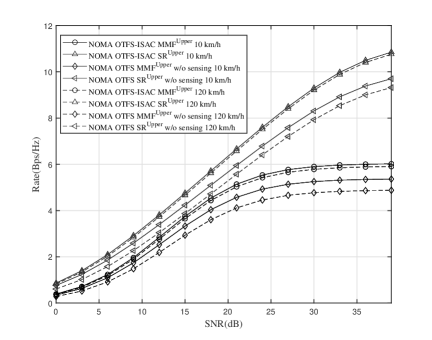
Figure 10: The comparison between MMF and SR under different speed with $e=0.02$.

Finally, the impact of speed on the system illustrated in Fig. 10 is investigated. Observations reveal that system performance decreases as the speed of the system increases. This decrease in performance is attributed to the widening of the position gap between the actual value and estimation of the system without sensing due to the higher speed. Moreover, the performance of the NOMA-OTFS system without sensing experiences a higher degradation. However, the incorporation of real-time motion prediction in the NOMA-assisted OTFS-ISAC results in a smaller degradation in performance. Additionally, the performance degradation in the presence of NLOS is less significant when the SNR exceeds 30 dB.

V Conclusion

In this paper, we proposed a novel NOMA-assisted OTFS-ISAC network, where a UAV serves as an air base station to support multiple users. The system employs the OTFS waveform to extract the user’s position and velocity information from the echo signals during communication. A three-dimensional motion model is proposed to retrieve the distance, velocity, and angle information of users from the echo signals. The impact of the NLOS channel on the robust power allocation is evaluated for two NOMA classic problems: maximum SR and MMF. The proposed NOMA-assisted OTFS-ISAC system is demonstrated to achieve superior achievable data performance over the benchmark systems in terms of SR and MMF under both perfect and imperfect channel assumptions.

References

- [1] S. N. Swamy and S. R. Kota, “An Empirical Study on System Level Aspects of Internet of Things (IoT),” IEEE Access, vol. 8, pp. 188 082–188 134, 2020.
- [2] C. Shi, Y. Wang, F. Wang, and H. Li, “Joint optimization of subcarrier selection and power allocation for dual-functional radar-communications system,” in 2020 IEEE 11th Sensor Array and Multichannel Signal Processing Workshop (SAM), 2020, pp. 1–5.
- [3] A. Liu, Z. Huang, M. Li, Y. Wan, W. Li, T. X. Han, C. Liu, R. Du, D. K. P. Tan, J. Lu, Y. Shen, F. Colone, and K. Chetty, “A survey on fundamental limits of integrated sensing and communication,” IEEE Communications Surveys Tutorials, vol. 24, no. 2, pp. 994–1034, 2022.
- [4] F. Liu, Y. Cui, C. Masouros, J. Xu, T. X. Han, Y. C. Eldar, and S. Buzzi, “Integrated sensing and communications: Toward dual-functional wireless networks for 6g and beyond,” IEEE Journal on Selected Areas in Communications, vol. 40, no. 6, pp. 1728–1767, 2022.
- [5] R. M. Mealey, “A method for calculating error probabilities in a radar communication system,” IEEE Transactions on Space Electronics and Telemetry, vol. 9, no. 2, pp. 37–42, 1963.
- [6] E. Fishler, A. Haimovich, R. Blum, D. Chizhik, L. Cimini, and R. Valenzuela, “MIMO radar: an idea whose time has come,” in Proceedings of the 2004 IEEE Radar Conference (IEEE Cat. No.04CH37509), 2004, pp. 71–78.
- [7] S. Fortunati, L. Sanguinetti, F. Gini, M. S. Greco, and B. Himed, “Massive MIMO radar for target detection,” IEEE Transactions on Signal Processing, vol. 68, pp. 859–871, 2020.
- [8] R. W. Heath, N. González-Prelcic, S. Rangan, W. Roh, and A. M. Sayeed, “An overview of signal processing techniques for millimeter wave MIMO systems,” IEEE Journal of Selected Topics in Signal Processing, vol. 10, no. 3, pp. 436–453, 2016.
- [9] C. Sturm and W. Wiesbeck, “Waveform design and signal processing aspects for fusion of wireless communications and radar sensing,” Proceedings of the IEEE, vol. 99, no. 7, pp. 1236–1259, 2011.
- [10] Y. Liu, G. Liao, and Z. Yang, “Range and angle estimation for MIMO-OFDM integrated radar and communication systems,” in 2016 CIE International Conference on Radar (RADAR), 2016, pp. 1–4.
- [11] Y. L. Sit and T. Zwick, “MIMO OFDM radar with communication and interference cancellation features,” in 2014 IEEE Radar Conference, 2014, pp. 0265–0268.
- [12] H. Qu, G. Liu, L. Zhang, S. Wen, and M. A. Imran, “Low-complexity symbol detection and interference cancellation for OTFS system,” IEEE Transactions on Communications, vol. 69, no. 3, pp. 1524–1537, 2021.
- [13] R. Hadani, S. Rakib, M. Tsatsanis, A. Monk, and R. Calderbank, “Orthogonal time frequency space modulation,” in IEEE Wireless Communications & Networking Conference, 2017.
- [14] P. Raviteja, K. T. Phan, Y. Hong, and E. Viterbo, “Interference cancellation and iterative detection for orthogonal time frequency space modulation,” IEEE Transactions on Wireless Communications, vol. 17, no. 10, pp. 6501–6515, 2018.
- [15] L. Gaudio, M. Kobayashi, G. Caire, and G. Colavolpe, “On the effectiveness of OTFS for joint radar and communication,” arXiv preprint arXiv:1910.01896, 2019.
- [16] L. Gaudio, M. Kobayashi, G. Caire, and G. Colavolpe, “Hybrid digital-analog beamforming and MIMO radar with OTFS modulation,” arXiv preprint arXiv:2009.08785, 2020.
- [17] K. Wu, J. A. Zhang, X. Huang, and Y. J. Guo, “OTFS-based joint communication and sensing for future industrial IoT,” 2021.
- [18] P. Raviteja, K. T. Phan, Y. Hong, and E. Viterbo, “Orthogonal time frequency space (OTFS) modulation based radar system,” in 2019 IEEE Radar Conference (RadarConf), 2019.
- [19] L. Gaudio, M. Kobayashi, G. Caire, and G. Colavolpe, “On the effectiveness of OTFS for joint radar parameter estimation and communication,” IEEE Transactions on Wireless Communications, vol. 19, no. 9, pp. 5951–5965, 2020.
- [20] F. Dong and F. Liu, “Localization as a service in perceptive networks: An ISAC resource allocation framework,” in 2022 IEEE International Conference on Communications Workshops (ICC Workshops), 2022, pp. 848–853.
- [21] W. Yuan, Z. Wei, S. Li, J. Yuan, and D. Ng, “Integrated sensing and communication-assisted orthogonal time frequency space transmission for vehicular networks,” 2021.
- [22] W. Yuan, S. Li, Z. Wei, J. Yuan, and D. W. Kwan Ng, “Bypassing channel estimation for otfs transmission: An integrated sensing and communication solution,” in 2021 IEEE Wireless Communications and Networking Conference Workshops (WCNCW), 2021, pp. 1–5.
- [23] Z. Wang, Y. Liu, X. Mu, Z. Ding, and O. A. Dobre, “NOMA empowered integrated sensing and communication,” IEEE Communications Letters, vol. 26, no. 3, pp. 677–681, 2022.
- [24] Z. Wang, Y. Liu, X. Mu, and Z. Ding, “NOMA inspired interference cancellation for integrated sensing and communication,” in ICC 2022 - IEEE International Conference on Communications, 2022, pp. 3154–3159.
- [25] Z. Ding, “Robust beamforming design for OTFS-NOMA,” IEEE Open Journal of the Communications Society, vol. 1, pp. 33–40, 2020.
- [26] K. Meng, D. Li, X. He, and M. Liu, “Space pruning based time minimization in delay constrained multi-task uav-based sensing,” IEEE Transactions on Vehicular Technology, vol. 70, no. 3, pp. 2836–2849, March 2021.
- [27] Z. Yu, X. Hu, C. Liu, M. Peng, and C. Zhong, “Location sensing and beamforming design for irs-enabled multi-user ISAC systems,” IEEE Transactions on Signal Processing, vol. 70, pp. 5178–5193, 2022.
- [28] J. Yuan, Y.-C. Liang, J. Joung, G. Feng, and E. G. Larsson, “Intelligent reflecting surface-assisted cognitive radio system,” IEEE Transactions on Communications, vol. 69, no. 1, pp. 675–687, 2021.
- [29] C.-L. Wang, Y.-C. Wang, and P. Xiao, “Power allocation based on sinr balancing for NOMA systems with imperfect channel estimation,” in 2019 13th International Conference on Signal Processing and Communication Systems (ICSPCS), 2019, pp. 1–6.
- [30] K. Deka, A. Thomas, and S. Sharma, “Otfs-scma: A code-domain noma approach for orthogonal time frequency space modulation,” IEEE Transactions on Communications, vol. 69, no. 8, pp. 5043–5058, 2021.
- [31] S. Lu, F. Liu, and L. Hanzo, “The degrees-of-freedom in monostatic isac channels: Nlos exploitation vs. reduction,” IEEE Transactions on Vehicular Technology, vol. 72, no. 2, pp. 2643–2648, 2023.
- [32] K. V. Rangarao and S. Venkatanarasimhan, “gold-music: A variation on music to accurately determine peaks of the spectrum,” IEEE Transactions on Antennas and Propagation, vol. 61, no. 4, pp. 2263–2268, 2013.
- [33] J. Wang, Y. Cui, H. Sun, X. Feng, G. Han, M. Wen, J. Li, and H. Esmaiel, “K-factor estimation for wireless communications over rician frequency-flat fading channels,” IEEE Wireless Communications Letters, vol. 10, no. 9, pp. 2037–2040, 2021.
- [34] J. Zhu, J. Wang, Y. Huang, S. He, X. You, and L. Yang, “On optimal power allocation for downlink non-orthogonal multiple access systems,” IEEE Journal on Selected Areas in Communications, vol. 35, no. 12, pp. 2744–2757, 2017.
- [35] Z. Yang, Z. Ding, P. Fan, and N. Al-Dhahir, “A general power allocation scheme to guarantee quality of service in downlink and uplink NOMA systems,” IEEE Transactions on Wireless Communications, vol. 15, no. 11, pp. 7244–7257, 2016.
- [36] N. S. Mouni, A. Kumar, and P. K. Upadhyay, “Adaptive user pairing for noma systems with imperfect sic,” IEEE Wireless Communications Letters, vol. 10, no. 7, pp. 1547–1551, 2021.
- [37] X. Chen, F.-K. Gong, G. Li, H. Zhang, and P. Song, “User pairing and pair scheduling in massive mimo-noma systems,” IEEE Communications Letters, vol. 22, no. 4, pp. 788–791, 2018.
- [38] L. Gaudio, M. Kobayashi, B. Bissinger, and G. Caire, “Performance analysis of joint radar and communication using OFDM and OTFS,” in 2019 IEEE International Conference on Communications Workshops (ICC Workshops), 2019, pp. 1–6.