Distributed Linear Regression with Compositional Covariates

Abstract

With the availability of extraordinarily huge data sets, solving the problems of distributed statistical methodology and computing for such data sets has become increasingly crucial in the big data area. In this paper, we focus on the distributed sparse penalized linear log-contrast model in massive compositional data. In particular, two distributed optimization techniques under centralized and decentralized topologies are proposed for solving the two different constrained convex optimization problems. Both two proposed algorithms are based on the frameworks of Alternating Direction Method of Multipliers (ADMM) and Coordinate Descent Method of Multipliers(CDMM, Lin et al., 2014, Biometrika). It is worth emphasizing that, in the decentralized topology, we introduce a distributed coordinate-wise descent algorithm based on Group ADMM(GADMM, Elgabli et al., 2020, Journal of Machine Learning Research) for obtaining a communication-efficient regularized estimation. Correspondingly, the convergence theories of the proposed algorithms are rigorously established under some regularity conditions. Numerical experiments on both synthetic and real data are conducted to evaluate our proposed algorithms.

Keywords: linear log-contrast model, GADMM, coordinate-wise descent, distributed computing, variable selection

1 Introduction

When one response variable is to be predicted by the proportions or fractions of a composition, regression models with compositional covariates are often used. A desirable regression association in terms of a log-contrast of compositional measurements was proposed by Aitchison and Bacon-Shone (1984). Suppose that the full data set $\mathscr{F}_{n}=\{(y_{i},\mathbbm{x}_{i}):i=1,\ldots,n\}$ consists of $n$ independent and identically distributed (i.i.d.) observations. Given a response $\boldsymbol{Y}=(y_{1},\ldots,y_{n})^{\top}\in\mathbbm{R}^{n}$, an $n\times p$ covariate matrix $\boldsymbol{X}=(X_{1},\ldots,X_{p})\in\mathbbm{R}^{n\times p}$ with the unit-sum constraint consists of $n$ observations of the composition of a mixture with $p$ components. That is, each covariate vector $\{\mathbbm{x}_{i}=(x_{i1},\ldots,x_{ip})^{\top}:i=1,\ldots,n\}$ of $\boldsymbol{X}$ lies in the $(p-1)-$dimensional positive Simplex

$$S^{p-1}=\left\{(x_{i1},\ldots,x_{ip})\mid x_{ij>0},\sum_{j=1}^{p}x_{ij}=1,j=1,\ldots,p\right\}.$$

The log-contrast or additive log-ratio transformation introduced by Aitchison (1982) is adopted to $\boldsymbol{X}$, i.e. $\boldsymbol{Z}_{-p}=(Z_{1},\ldots,Z_{p-1})=\left(\log\frac{X_{1}}{X_{p}},\ldots,\log\frac{X_{p-1}}{X_{p}}\right),$ where $\boldsymbol{Z}_{-p}$ is the $n\times(p-1)$ log-ratio matrix. Correspondingly, the linear log-contrast model is formulated as follows

$$\boldsymbol{Y}=\boldsymbol{Z}_{-p}\boldsymbol{\beta}_{-p}+\boldsymbol{\epsilon},$$ (1)

where $\boldsymbol{\beta}_{-p}=(\beta_{1},\ldots,\beta_{p-1})^{\top}$ is the regression coefficient that need to be estimated and $\boldsymbol{\epsilon}=(\epsilon_{1},\ldots,\epsilon_{n})^{\top}$ is the independent random error vector. Notice that it is crucial to investigate the variable selection and estimation procedures for (1). To select the important variables from all components including reference component more conveniently, Lin et al. (2014) re-expressed the model (1) by setting $\beta_{p}=-\sum_{j=1}^{p-1}\beta_{j}$ as a zero-sum constraint, that is

$$\boldsymbol{Y}=\boldsymbol{Z}\boldsymbol{\beta}+\boldsymbol{\epsilon},\leavevmode\nobreak\ \text{subject}\leavevmode\nobreak\ \text{to}\leavevmode\nobreak\ \sum_{j=1}^{p}\beta_{j}=0,$$ (2)

where $\boldsymbol{Z}=(Z_{1},\ldots,Z_{p})=(\log x_{ij})\in\mathbbm{R}^{n\times p}$, $\boldsymbol{\beta}=(\beta_{1},\ldots,\beta_{p})^{\top}$. Specifically, Lin et al. (2014) solve the following penalized optimization problem by using Coordinate Descent Method of Multipliers(CDMM)

$$\boldsymbol{\widehat{\beta}}=\arg\min\limits_{\boldsymbol{\beta}}\left(\frac{1}{2n}\|\boldsymbol{Y}-\boldsymbol{Z}\boldsymbol{\beta}\|^{2}+\lambda\|\boldsymbol{\beta}\|_{1}\right),\leavevmode\nobreak\ \text{subject}\leavevmode\nobreak\ \text{to}\leavevmode\nobreak\ \sum_{j=1}^{p}\beta_{j}=0,$$ (3)

where $\lambda$ is a regularization parameter.

There exist many statistical achievements for further solving the regularization problems with compositional or subcompositional data in analysis of microbiome data(Shi et al. (2016); Wang and Zhao (2017); Cao et al. (2019); Lu et al. (2019); Mishra and Müller (2022); Han et al. (2022)). For example, Shi et al. (2016) improved the linear regression model by including several linear constraints to achieve subcompositional coherence and developed a penalized estimation methodology for selecting relevant variables and estimating the regression coefficients. Wang and Zhao (2017) proposed the Tree-guided Automatic Subcomposition Selection Operator(TASSO) for conducting the tree-structured subcomposition selection and parameter estimation procedures. To tackle the issue of covariance estimation for high-dimensional compositional data, a composition-adjusted thresholding(COAT) method has been investigated by Cao et al. (2019). Without requiring the restrictive Gaussian or sub-Gaussian assumption, Li et al. (2022) further suggested the robust composition adjusted thresholding covariance procedure based on Huber-type M-estimation(M-COAT) to estimate the sparse covariance structure of high-dimensional compositional data. For the generalized linear models with high-dimensional compositional variables, Lu et al. (2019) developed a generalized accelerated proximal gradient algorithm to compute the estimates of regression coefficients and the statistical inference have been taken into consideration. Under the regression frameworks when containing both compositional and non-compositional covariates, Mishra and Müller (2022) proposed the Robust log-contrast Regression estimators with Compositional Covariates (RobRegCC) procedure for outlier detection and variable selection. When the error distribution was asymmetric and heavy-tailed, Han et al. (2022) provided a robust signal recovery strategy for high-dimensional linear log-contrast models. For more articles on compositional data analysis, we refer to a review paper by Alenazi (2021).

Nevertheless, when compositional data sets have extremely large sample size, the aforementioned techniques are unable to handle such massive data sets in a single standalone machine due to the heavy burden on storage and limited computing resources. In recent years, many contributions for dealing with non-compositional massive data sets have been arisen by the researchers in the context of statistical computing and inference. A popular way is that such data sets are usually divided across multiple connected machines and calculated by many communication-efficient algorithms corresponding to different statistical problems(Tan et al. (2022); Fan et al. (2021); Zhang et al. (2013); Huang et al. (2021); Liu et al. (2023); Zhou et al. (2021); Li and Zhao (2022); Shi et al. (2021); Jordan et al. (2019); Yang and Wang (2023); Ma et al. (2022), etc). Among them, the distributed communication-efficient surrogate likelihood (CSL) framework proposed by Jordan et al. (2019) aims for estimation and inference in low-dimensional regression, high-dimensional variable selection and Bayesian statistics. It has been widely extended to various aspects including linear regression(Liu et al. (2023); Fan et al. (2021)), quantile regression(Hu et al. (2021); Wang et al. (2022a); Tan et al. (2022),etc.), composite quantile regression(Yang and Wang (2023); Wang et al. (2021)), modal regression(Wang et al. (2021)), expectile regression(Pan (2021)), Huber regression(Pan et al. (2022)), neural network(Wang et al. (2022b)), etc. In high-dimensional settings, the estimation and variable selection procedures rather than CSL frameworks have simultaneously considered under the distributed system, refer to Chen et al. (2020); Zhou et al. (2021); Gu and Zou (2020); Fan and Fan (2023); Yu et al. (2017); Volgushev et al. (2019); Zhu et al. (2021); Yu et al. (2022), etc. The divide-and-conquer methods for solving distributed system problems are summarized in a review paper provided by Gao et al. (2022). It is worth pointing out that the optimization algorithms in the above-mentioned literature for the distributed data are mainly based on the frameworks of proximal Alternating Direction Method of Multipliers(ADMM, Boyd et al. (2011)). In addition, they solve the problems in a centralized regime. In other words, there exists a master machine, which has a link to each local machine. To obtain a global optimal solution, the master machine collects the current local estimators calculated on the node machines after local parameter updating iteratively. Then, the aggregating parameter estimators are transmitted to the local machine for the next iteration.

However, such master-worker distributed framework has several drawbacks. First, the master machine is vulnerable to attackers. As a result, all informative updates from local machines that sends to the master machine can be easily obtained by attackers, which makes privacy unprotected(Wu et al. (2022)). Second, for robust operation, this centralized topology is quite fragile. In other words, if the master machine fails to work then the entire distributed system stops working. Third, due to the limited communication resources for the hardware devices in practice, the master node may require high quality for the communication network as the number of local machine grows large, which leads to the high communication cost among master machine and local workers. In addition, the issues that a large number of local machines are linked to a central machine and transmit the updated models to the central machine are unrealistic due to the limited computing power and high economic cost. More potential challenges for the master-worker distributed framework also can be found in Nedić et al. (2018); Wu et al. (2022); Elgabli et al. (2020a), etc.

To overcome these drawbacks, a number of researchers develop the efficient distributed algorithms in the decentralized topology(Nedić et al. (2018); Elgabli et al. (2020a); Issaid et al. (2020); Atallah et al. (2022); Elgabli et al. (2020b); Wu et al. (2022), etc). Especially, Group Alternating Direction Method of Multipliers(GADMM, Elgabli et al. (2020a)) is an extension to the framework of ADMM. Suppose that there exist $K$ machines. As introduced in Elgabli et al. (2020a), GADMM algarithm aims to solve the optimization problem $\frac{1}{K}\sum_{k=1}^{K}f_{k}(\boldsymbol{\alpha}_{k})$ with constraints $\boldsymbol{\alpha}_{k}=\boldsymbol{\alpha}_{k+1},\leavevmode\nobreak\ k=1,\ldots,K-1$, where $f_{k}(\cdot)$ is the local convex, proper, and closed function. The basic principle is that the machines are split into two groups, head and tail, with each machine in the head(tail) group communicating solely with its two neighboring machines in the tail(head) group.

The previous works mainly focus on the distributed optimization problems with only one type of constraints. Moreover, the original GADMM algorithm as a model-free approach can only solve the parameter estimation problem without any regularization consideration for variable selection problem. In this paper, we consider the distributed estimation and variable selection procedures for model (2) including non-compositional covariates and two types of constraints under the centralized and decentralized manners, which fills the gap in the fields of massive compositional data analysis. Correspondingly, we develop a efficient distributed optimization algorithms in the frameworks of ADMM and CDMM to solve the penalized linear log-contrast regression models with the LASSO(Tibshirani (1996)), adaptive LASSO(Zou (2006)), and SCAD(Fan and Li (2001)) penalties. More specifically, inspired by the idea of GADMM algorithm, we introduce a distributed sparse group coordinate descent method of multipliers(DSGCDMM) for solving the two constrained optimization problem in a decentralized framework. Meanwhile, the convergence theories are established for the proposed methodologies under some assumptions.

The remainder of the paper is organized as follows. Section 2 introduces a general framework for distributed penalized linear regression with compositional covariates and presents the related algorithm in a centralized regime. Section 3 presents a decentralized algorithm for the variable selection procedure in a distributed framework. The regularization parameter selection are presented in Section 3.2. In Section 4, we present the convergence theories. Simulation experiments and real data analysis in Section 5 are conducted to demonstrate the numerical and statistical efficiency of the proposed two variable selection procedures. Finally, we conclude this article with some discussions in Section 6. All technical details and additional numerical results are delegated to the Appendix.

2 A General Framework

We begin by setting up our distributed regime for penalized large-scale linear regression with compositional covariates, after which we turn to a detailed description of the distributed variable selection procedure in a master-worker system.

2.1 Distributed Penalized Linear Regression with Compositional Covariates

We now investigate the distributed statistical scheme for quantifying the relationship between response and compositional covariates under a master-worker framework. Without losing generality and simplicity, we assume that the response and explanatory variables are centered. In practice, compositional covariates together with $q$ additional non-compositional covariates $\boldsymbol{V}=(V_{1},\ldots,V_{q})\in\mathbbm{R}^{n\times q}$ are often appeared in regression analysis. Following the argument of Mishra and Müller (2022), we consider a extended linear log-contrast model based on (2) as presented below

$$\begin{split}\boldsymbol{Y}&=\boldsymbol{Z}\boldsymbol{\beta}+\boldsymbol{V}\boldsymbol{\theta}+\boldsymbol{\epsilon}\\ &\equiv\boldsymbol{\Pi}\boldsymbol{\zeta}+\boldsymbol{\epsilon},\leavevmode\nobreak\ \text{subject}\leavevmode\nobreak\ \text{to}\leavevmode\nobreak\ \boldsymbol{C}^{\top}\boldsymbol{\zeta}=0,\end{split}$$ (4)

where $\boldsymbol{\Pi}=(\boldsymbol{Z},\boldsymbol{V})$, $\boldsymbol{\zeta}=(\boldsymbol{\beta}^{\top},\boldsymbol{\theta}^{\top})^{\top}$, $\boldsymbol{C}=(\boldsymbol{1}_{p}^{\top},\boldsymbol{0}_{q}^{\top})^{\top}\in\mathbbm{R}^{(p+q)}$ with $\boldsymbol{1}_{p}=(1,\ldots,1)^{\top}\in\mathbbm{R}^{p}$ and $\boldsymbol{0}_{q}=(0,\ldots,0)^{\top}\in\mathbbm{R}^{q}$.

Let $d=p+q$. For a distributed system, the full data set $\mathscr{F}_{n}$ are partitioned across $K$ servers(machines) $\{\mathscr{M}_{k}\}_{k=1}^{K}$. Then,

$$\boldsymbol{Y}=(\boldsymbol{y}^{\top}_{1},\ldots,\boldsymbol{y}^{\top}_{K})^{\top},$$

$$\leavevmode\nobreak\ \text{and}\leavevmode\nobreak\ \text{correspondingly}\\ \leavevmode\nobreak\ \boldsymbol{\Pi}=(\boldsymbol{\Pi}_{1}^{\top},\ldots,\boldsymbol{\Pi}_{K}^{\top})^{\top},$$

where $\boldsymbol{y}_{k}\in\mathbbm{R}^{n_{k}}$, $\boldsymbol{\Pi}_{k}=(\boldsymbol{\pi}_{k,1},\ldots,\boldsymbol{\pi}_{k,d})\in\mathbbm{R}^{n_{k}\times d}$, and $\sum_{k=1}^{K}n_{k}=n$. In such settings, we consider following constrained convex optimization problem in a master-worker framework by applying weighted $L_{1}-$penalized regularization approach to model (4),

$$\begin{split}\widetilde{\boldsymbol{\zeta}}&=\underset{\boldsymbol{\zeta},\{\boldsymbol{\zeta}_{k}\}^{K}_{k=1}}{\operatorname{argmin}}\sum_{k=1}^{K}\frac{1}{2n_{k}}\|\boldsymbol{y}_{k}-\boldsymbol{\Pi}_{k}\boldsymbol{\zeta}_{k}\|^{2}+\lambda\|\boldsymbol{\omega}\circ\boldsymbol{\zeta}\|_{1},\\ &\text{subject}\leavevmode\nobreak\ \text{to}\leavevmode\nobreak\ \begin{cases}\boldsymbol{C}^{\top}\boldsymbol{\zeta}=0,\\ \boldsymbol{\zeta}_{k}=\boldsymbol{\zeta},\end{cases}k=1,\ldots,K,\end{split}$$ (5)

where $\boldsymbol{\zeta}$ is the global model parameter. Here, for $\mathscr{M}_{k}$, $\boldsymbol{\zeta}_{k}=(\zeta_{k,1},\ldots,\zeta_{k,d})^{\top}$ is the coefficient vector with respect to split data $\{\boldsymbol{y}_{k},\boldsymbol{\Pi}_{k}\}$, $\lambda$ is a regularization parameter that dictates the size of model (4), the vector $\boldsymbol{\omega}=(\omega_{1},\ldots,\omega_{d})^{\top}$ consists of pre-specified nonnegative weights, and $\|\boldsymbol{\omega}\circ\boldsymbol{\zeta}\|_{1}=\sum_{j=1}^{d}\omega_{j}|\zeta_{j}|$ with $\circ$ standing for the Hadamard product. It is worth mentioning that $\|\boldsymbol{\omega}\circ\boldsymbol{\zeta}\|_{1}$ in formulation (5) is a general form for the $L_{1}-$penalized regression with constraints. Instead, for the LASSO penalty, $\boldsymbol{\omega}$ can be specified as $\boldsymbol{\omega}=\boldsymbol{1}_{d}$, where $\boldsymbol{1}_{d}=(1,\ldots,1)^{\top}\in\mathbbm{R}^{d}$. While for the adaptive LASSO penalty, $\boldsymbol{\omega}=\left((|\widetilde{\zeta}_{j}^{\text{LASSO}}|+\frac{1}{n})^{-1},j=1\ldots,d\right)^{\top}$ as a generalization of the LASSO penalty is commonly used, where $\widetilde{\boldsymbol{\zeta}}^{\text{LASSO}}=\left(\widetilde{\zeta}_{j}^{\text{LASSO}},j=1,\ldots,d\right)^{\top}$ is the LASSO estimator in Lin et al. (2014). If we consider the nonconvex penalty, then SACD weight $\boldsymbol{\omega}=\left(\lambda^{-1}p_{\lambda}^{\prime}(|\overline{\zeta}_{j}|),j=1,\ldots,d\right)^{\top}$ is usually employed(Zou and Li (2008); Liu et al. (2023)), where $p_{\lambda}^{\prime}(|u|)=\lambda I(|u|\leq\lambda)+\frac{(a\lambda-|u|)_{+}}{(a-1)I(|u|>\lambda)}$ for some $a>2$. As suggested in Fan and Li (2001), often $a=3.7$ is a considerable choice. According to Zou and Li (2008), local linear approximation(LLA) algorithm can effectively solve the SCAD-penalized regression. In this work, $\overline{\boldsymbol{\zeta}}=\left(\overline{\zeta}_{j},j=1,\ldots,d\right)^{\top}$ is replaced by the current $m_{th}$ iteration $\boldsymbol{\zeta}^{m}$ in the local machines, and LLA algorithm repeatedly calculate the following constrained nonconvex optimization

$$\begin{split}\boldsymbol{\zeta}^{m+1}&=\underset{\boldsymbol{\zeta},\{\boldsymbol{\zeta}_{k}\}^{K}_{k=1}}{\operatorname{argmin}}\sum_{k=1}^{K}\frac{1}{2n_{k}}\|\boldsymbol{y}_{k}-\boldsymbol{\Pi}_{k}\boldsymbol{\zeta}_{k}\|^{2}+\sum_{j=1}^{d}p_{\lambda}^{\prime}(|{\zeta}^{m}_{j}|)|\zeta_{j}|,\\ &\text{subject}\leavevmode\nobreak\ \text{to}\leavevmode\nobreak\ \begin{cases}\boldsymbol{C}^{\top}\boldsymbol{\zeta}=0,\\ \boldsymbol{\zeta}_{k}=\boldsymbol{\zeta},\end{cases}k=1,\ldots,K.\end{split}$$ (6)

In the next subsection, we will introduce a distributed algorithm in a centralized framework for solving problem (5). The problem (6) can be also solved by combining the LLA algorithm and coordinate descent(CD) algorithm(Breheny and Huang (2011)) together with the distributed algorithm.

2.2 A Distributed Sparse Coordinate Descent Method of Multipliers

We now introduce a centralized algorithm, i.e. distributed sparse coordinate descent method of multipliers(DSCDMM), to solve the weighted $L_{1}-$ penalized linear regression with compositional covariates in big data. Notice that there exist two kinds of constraints in the optimization problem (5). To address this kind of convex optimization problem with several convex constraints, Giesen and Laue (2019) proposed a extended approach for ADMM(Boyd et al. (2011)), i.e. combine the superiority of ADMM to calculate the convex optimization problems in a distributed regime with the advantage of the augmented Lagrangian method to overcome constrained optimization problems. Inspired by Giesen and Laue (2019), pick penalty parameter $\rho>0$ and denote $\boldsymbol{C}=(c_{1},\ldots,c_{d})^{\top}$, we consider the augmented Lagrangian for the optimization problem in (5) as

$$\begin{split}\mathscr{L}_{\rho}\left(\{\boldsymbol{\zeta}_{k}\}^{K}_{k=1},\mu,\{\boldsymbol{\gamma}_{k}\}_{k=1}^{K}\right)=&\sum_{k=1}^{K}\frac{1}{2n_{k}}\|\boldsymbol{y}_{k}-\boldsymbol{\Pi}_{k}\boldsymbol{\zeta}_{k}\|^{2}+\lambda\|\boldsymbol{\omega}\circ\boldsymbol{\zeta}\|_{1}+\sum_{j=1}^{d}\mu c_{j}\zeta_{j}\\ &+\frac{\rho}{2}\left(\sum_{j=1}^{d}c_{j}\zeta_{j}\right)^{2}+\sum_{k=1}^{K}\left\langle\boldsymbol{\gamma}_{k},\boldsymbol{\zeta}_{k}-\boldsymbol{\zeta}\right\rangle+\frac{\rho}{2}\sum_{k=1}^{K}\|\boldsymbol{\zeta}_{k}-\boldsymbol{\zeta}\|^{2},\end{split}$$ (7)

where $\mu\in\mathbbm{R}^{1}$ and $\boldsymbol{\gamma}_{k}\in\mathbbm{R}^{d}$ present the Lagrangian multipliers or dual variables, $\left\langle\cdot,\cdot\right\rangle$ and $\|\cdot\|$ stand for the inner product and $L_{2}-$norm in Euclidean space, respectively. Following Lin et al. (2014) and Elgabli et al. (2020a), for each machine $\mathscr{M}_{k}$, the updates of the primal and dual variables under the method of multipliers are given by

$$\begin{split}\boldsymbol{\zeta}_{k}^{l+1}:=\underset{\boldsymbol{\zeta}_{k}}{\operatorname{argmin}}&\frac{1}{2n_{k}}\|\boldsymbol{y}_{k}-\boldsymbol{\Pi}_{k}\boldsymbol{\zeta}_{k}\|^{2}+\left\langle\boldsymbol{\gamma}_{k}^{l},\boldsymbol{\zeta}_{k}-\boldsymbol{\zeta}^{l}\right\rangle+\frac{\rho}{2}\|\boldsymbol{\zeta}_{k}-\boldsymbol{\zeta}^{l}\|^{2},\end{split}$$ (8)

$$\boldsymbol{\zeta}^{l+1}:=\underset{\boldsymbol{\zeta}}{\operatorname{argmin}}\leavevmode\nobreak\ \lambda\|\boldsymbol{\omega}\circ\boldsymbol{\zeta}\|_{1}+\sum_{k=1}^{K}\left\langle\boldsymbol{\gamma}_{k}^{l},\boldsymbol{\zeta}_{k}^{l+1}-\boldsymbol{\zeta}\right\rangle+\frac{\rho}{2}\sum_{k=1}^{K}\|\boldsymbol{\zeta}_{k}^{l+1}-\boldsymbol{\zeta}\|^{2}+\sum_{j=1}^{d}\mu c_{j}\zeta_{j}+\frac{\rho}{2}\left(\sum_{j=1}^{d}c_{j}\zeta_{j}\right)^{2},$$ (9)

$$\mu^{l+1}\leftarrow\mu^{l}+\rho\sum_{j=1}^{d}c_{j}\zeta_{j}^{l+1},$$ (10)

$$\boldsymbol{\gamma}_{k}^{l+1}\leftarrow\boldsymbol{\gamma}_{k}^{l}+\rho(\boldsymbol{\zeta}_{k}^{l+1}-\boldsymbol{\zeta}^{l+1}).$$ (11)

The update of each $\boldsymbol{\zeta}_{k}^{l+1}$ can be rewritten as the form of a Tikhonov-regularized least squares(i.e., ridge regression):

$$\boldsymbol{\zeta}_{k}^{l+1}:=\underset{\boldsymbol{\zeta}_{k}}{\operatorname{argmin}}\frac{1}{2n_{k}}\|\boldsymbol{y}_{k}-\boldsymbol{\Pi}_{k}\boldsymbol{\zeta}_{k}\|^{2}+\frac{\rho}{2}\|\boldsymbol{\zeta}_{k}-\boldsymbol{\zeta}^{l}+\frac{1}{\rho}\boldsymbol{\gamma}^{l}_{k}\|^{2},$$

which has the analytical solution:

$$\boldsymbol{\zeta}_{k}^{l+1}\leftarrow(\frac{1}{n_{k}}\boldsymbol{\Pi}_{k}^{\top}\boldsymbol{\Pi}_{k}+\rho\boldsymbol{I})^{-1}(\frac{1}{n_{k}}\boldsymbol{\Pi}_{k}^{\top}\boldsymbol{y}_{k}+\rho\boldsymbol{\zeta}^{l}-\boldsymbol{\gamma}^{l}_{k}).$$ (12)

In general, updating $\boldsymbol{\zeta}$ in the subproblem (9) is challenging due to the nondifferentiable $L_{1}$ terms and non-closed form solution under the zero-sum constraint. To solve this type of problems, a class of efficient and fast algorithms named coordinate-wise descent algorithms are proposed by Friedman et al. (2007). Furthermore, Lin et al. (2014) and Gu et al. (2018) combine the coordinate descent algorithm with the method of multipliers or the augmented Lagrangian method to solve the LASSO-type high-dimensional linear regression with compositional covariates and quantile regression. Hence, we prefer to apply the coordinate descent algorithm to the $\boldsymbol{\zeta}$ updates in the distributed ADMM algorithm. We coordinate-wisely solve the subproblem (9) via updating following iterations

$$\begin{split}&\boldsymbol{\zeta}^{l,b+1}\leftarrow\\ &\left[\frac{\text{Shrink}\left\{\frac{1}{\rho}\sum_{k=1}^{K}\gamma_{k,j}^{l}+\sum_{k=1}^{K}\zeta_{k,j}^{l+1}-\frac{1}{\rho}\mu^{l}c_{j}-c_{j}\sum_{m\neq j}c_{m}\zeta_{m}^{l,b+I(m<j)},\frac{\lambda\omega_{j}}{\rho}\right\}}{(c_{j}^{2}+K)}\right]_{1\leq j\leq d},\end{split}$$ (13)

where $\text{Shrink}[\mu,\vartheta]=\text{sgn}(\mu)(|\mu|-\vartheta)_{+}$ is the soft thresholding operator. We subsequently propose the distributed sparse coordinate descent method of multipliers(DSCDMM) for solving large-scale penalized linear regression with compositional covariates, which is summarized in Algorithm 1.

Algorithm 1 DSCDMM: Distributed sparse coordinate descent method of multipliers for solving large-scale penalized linear regression with compositional covariates.

0:  Data $\{\boldsymbol{y}_{k},\boldsymbol{\Pi}_{k}\}_{k=1}^{K}$ on machines $\{\mathscr{M}_{k}\}_{k=1}^{K}$, the value of constant $\rho$, the number of rounds of communication $L$.

0:  $\boldsymbol{\zeta}^{L}$.

1:  Initialization:

• Set $\mathscr{M}_{1}$ as the master machine.

• $\boldsymbol{\zeta}_{k}^{0}=\boldsymbol{\gamma}_{k}^{0}$, $\mu_{k}^{0}=0$ for all $k$.

• Calculate $\boldsymbol{\omega}$ in the first machine.

2:  for $l=0,1,2,\ldots,L-1$ do

3:     For each local machine, update (12) in parallel.

4:     Carry out the coordinate descent Steps in master machine until the convergence criterion is met.

5:     Initialize $\boldsymbol{\zeta}^{l+1,0}=\boldsymbol{\zeta}^{l}$.

6:     for $b=0,1,2,\ldots$ do

7:        for $j=1,\ldots,d$ do

8:           Update $\zeta_{j}^{l,b+1}$ via (13).

9:        end for

10:        Set $\boldsymbol{\zeta}^{l+1}=\boldsymbol{\zeta}^{l,B}$.

11:     end for

12:     The master machine updates the dual variable $\mu^{l+1}$ via (10). Broadcast $\boldsymbol{\zeta}^{l+1}$ to other local machines.

13:     Every machine locally updates the dual variable $\boldsymbol{\gamma}_{k}^{l+1}$ (11).

14:  end for

3 A Decentralized Algorithm

It should be noted that algorithm 1 aims to solve the optimization problem in a centralized manner. That is, in each iteration, DSCDMM requires a master machine being connected to every node machine, then node machines calculate the local updates in parallel and send the updated variables to the master machine or central processor. After that, master machine broadcasts the aggregated parameters to node machines for new updates. However, when the number of machines increases, the above-mentioned variable selection procedure may results in heavy computation burden and limited communication resources for master machine. Even worse, we can not address a large communication network size that the master machine can be connected to all other local machines.

The GADMM was first introduced by Elgabli et al. (2020a). The core idea of the GADMM is to divide a group for all node machines connected with a chain into two groups(head group and tail group), then each machine in the head(or tail) group only communicates with two neighboring machines in the tail(or head) group to connect other machines except for the edge machines(first and last machines). Without losing generality, the number of machines is considered as even $K$ in the decentralized framework. Compared to the master-worker distributed ADMM, GADMM has the advantage that it only requires ${K}/{2}$ machines to carry out computation in parallel, so it effectively reduces the communication cost required by each machine. More technical details and convergence results are discussed in the Elgabli et al. (2020a). However, the GADMM algorithm can not be directly applied to computing the distributed penalized linear regression with compositional covariates in a decentralized regime due to the difficult and complex optimization problem with two different constraints and weighted $L_{1}$-penalized regularization problems. In the next subsection, we will solve these intractable problems systematically.

3.1 A Distributed Sparse Group Coordinate Descent Method of Multipliers

In this subsection, we will construct the variable selection procedure for the massive linear regression with compositional covariates in a decentralized manner, which aims to solve the issue with the whole data distributed across $K$ machines $\{\mathscr{M}_{k}\}_{k=1}^{K}$ and allow the communication of each machine to connect only two neighbors. To derive the fast and communication-efficient algorithm for dealing with the above-mentioned procedure, we reformulate the weighted optimization problem with two kinds of constraints in (5) as follows

$$\begin{split}\widehat{\boldsymbol{\zeta}}&=\underset{\{\boldsymbol{\zeta}_{k}\}_{k=1}^{K}}{\operatorname{argmin}}\sum_{k=1}^{K}\left\{\frac{1}{2n_{k}}\|\boldsymbol{y}_{k}-\boldsymbol{\Pi}_{k}\boldsymbol{\zeta}_{k}\|^{2}+\lambda\|\boldsymbol{\omega}_{k}\circ\boldsymbol{\zeta}_{k}\|_{1}\right\},\\ &\text{subject}\leavevmode\nobreak\ \text{to}\leavevmode\nobreak\ \begin{cases}\boldsymbol{C}^{\top}\boldsymbol{\zeta}_{k}=0,\\ \boldsymbol{\zeta}_{k}=\boldsymbol{\zeta}_{k+1},\end{cases}k=1,\ldots,K-1.\end{split}$$ (14)

Analogously to GADMM and the literature Giesen and Laue (2019), for the penalty parameter $\rho>0$, our extension work on the augmented Lagrangian function for problem (14) is given by

$$\begin{split}\mathscr{L}_{\rho}\big{(}\{\boldsymbol{\zeta}_{k}\}^{K}_{k=1},&\{\mu_{k}\}_{K=1}^{K},\{\boldsymbol{\gamma}_{k}\}_{k=1}^{K}\big{)}=\sum_{k=1}^{K}\left\{\frac{1}{2n_{k}}\|\boldsymbol{y}_{k}-\boldsymbol{\Pi}_{k}\boldsymbol{\zeta}_{k}\|^{2}+\lambda\|\boldsymbol{\omega}_{k}\circ\boldsymbol{\zeta}_{k}\|_{1}\right\}+\sum_{k=1}^{K}\sum_{j=1}^{d}\mu_{k}c_{j}\zeta_{k,j}\\ &+\frac{\rho}{2}\sum_{k=1}^{K}\left(\sum_{j=1}^{d}c_{j}\zeta_{k,j}\right)^{2}+\sum_{k=1}^{K}\left\langle\boldsymbol{\gamma}_{k},\boldsymbol{\zeta}_{k}-\boldsymbol{\zeta}_{k+1}\right\rangle+\frac{\rho}{2}\sum_{k=1}^{K}\|\boldsymbol{\zeta}_{k}-\boldsymbol{\zeta}_{k+1}\|^{2},\end{split}$$ (15)

where $\mu_{k}\in\mathbbm{R}^{1}$ and $\boldsymbol{\gamma}_{k}\in\mathbbm{R}^{d}$ present the Lagrangian multipliers or dual variables. Let $\mathscr{N}_{h}=\{\mathscr{M}_{1},\mathscr{M}_{3},\ldots,\mathscr{M}_{K-1}\}$ and $\mathscr{N}_{t}=\{\mathscr{M}_{2},\mathscr{M}_{4},\ldots,\mathscr{M}_{K}\}$ denote the collections of machines in head group and tail group, respectively. Correspondingly, at iteration $l+1$, the updating rules for primal variables in the head group can be written as

$$\begin{split}&\boldsymbol{\zeta}_{k}^{l+1}:=\arg\min_{\boldsymbol{\zeta}_{k}}\frac{1}{2n_{k}}\|\boldsymbol{y}_{k}-\boldsymbol{\Pi}_{k}\boldsymbol{\zeta}_{k}\|^{2}+\lambda\|\boldsymbol{\omega}_{k}\circ\boldsymbol{\zeta}_{k}\|_{1}\\ &\leavevmode\nobreak\ \leavevmode\nobreak\ \leavevmode\nobreak\ \leavevmode\nobreak\ \leavevmode\nobreak\ \leavevmode\nobreak\ \leavevmode\nobreak\ \leavevmode\nobreak\ \leavevmode\nobreak\ \leavevmode\nobreak\ \leavevmode\nobreak\ \leavevmode\nobreak\ \leavevmode\nobreak\ \leavevmode\nobreak\ \leavevmode\nobreak\ \leavevmode\nobreak\ \leavevmode\nobreak\ \leavevmode\nobreak\ \leavevmode\nobreak\ +\mu_{k}^{l}\sum_{j=1}^{d}c_{j}\zeta_{k,j}+\frac{\rho}{2}(\sum_{j=1}^{d}c_{j}\zeta_{k,j})^{2}\\ &\leavevmode\nobreak\ \leavevmode\nobreak\ \leavevmode\nobreak\ \leavevmode\nobreak\ \leavevmode\nobreak\ \leavevmode\nobreak\ \leavevmode\nobreak\ \leavevmode\nobreak\ \leavevmode\nobreak\ \leavevmode\nobreak\ \leavevmode\nobreak\ \leavevmode\nobreak\ \leavevmode\nobreak\ \leavevmode\nobreak\ \leavevmode\nobreak\ \leavevmode\nobreak\ \leavevmode\nobreak\ \leavevmode\nobreak\ \leavevmode\nobreak\ +\left\langle\boldsymbol{\gamma}_{k}^{l},\boldsymbol{\zeta}_{k}-\boldsymbol{\zeta}_{k+1}^{l}\right\rangle+\frac{\rho}{2}\|\boldsymbol{\zeta}_{k}-\boldsymbol{\zeta}_{k+1}^{l}\|^{2},\leavevmode\nobreak\ k=1.\end{split}$$ (16)

$$\begin{split}&\boldsymbol{\zeta}_{k}^{l+1}:=\arg\min_{\boldsymbol{\zeta}_{k}}\frac{1}{2n_{k}}\|\boldsymbol{y}_{k}-\boldsymbol{\Pi}_{k}\boldsymbol{\zeta}_{k}\|^{2}+\lambda\|\boldsymbol{\omega}_{k}\circ\boldsymbol{\zeta}_{k}\|_{1}+\mu_{k}^{l}\sum_{j=1}^{d}c_{j}\zeta_{k,j}+\frac{\rho}{2}(\sum_{j=1}^{d}c_{j}\zeta_{k,j})^{2}\\ &\leavevmode\nobreak\ \leavevmode\nobreak\ \leavevmode\nobreak\ \leavevmode\nobreak\ \leavevmode\nobreak\ \leavevmode\nobreak\ \leavevmode\nobreak\ \leavevmode\nobreak\ \leavevmode\nobreak\ \leavevmode\nobreak\ \leavevmode\nobreak\ \leavevmode\nobreak\ \leavevmode\nobreak\ \leavevmode\nobreak\ \leavevmode\nobreak\ \leavevmode\nobreak\ \leavevmode\nobreak\ \leavevmode\nobreak\ \leavevmode\nobreak\ +\left\langle\boldsymbol{\gamma}_{k-1}^{l},\boldsymbol{\zeta}_{k-1}^{l}-\boldsymbol{\zeta}_{k}\right\rangle+\left\langle\boldsymbol{\gamma}_{k}^{l},\boldsymbol{\zeta}_{k}-\boldsymbol{\zeta}_{k+1}^{l}\right\rangle\\ &\leavevmode\nobreak\ \leavevmode\nobreak\ \leavevmode\nobreak\ \leavevmode\nobreak\ \leavevmode\nobreak\ \leavevmode\nobreak\ \leavevmode\nobreak\ \leavevmode\nobreak\ \leavevmode\nobreak\ \leavevmode\nobreak\ \leavevmode\nobreak\ \leavevmode\nobreak\ \leavevmode\nobreak\ \leavevmode\nobreak\ \leavevmode\nobreak\ \leavevmode\nobreak\ \leavevmode\nobreak\ \leavevmode\nobreak\ \leavevmode\nobreak\ +\frac{\rho}{2}\|\boldsymbol{\zeta}_{k-1}^{l}-\boldsymbol{\zeta}_{k}\|^{2}+\frac{\rho}{2}\|\boldsymbol{\zeta}_{k}-\boldsymbol{\zeta}_{k+1}^{l}\|^{2},\leavevmode\nobreak\ k\in\mathscr{N}_{h}\backslash\{1\}.\end{split}$$ (17)

Send the updates $\boldsymbol{\zeta}_{k}^{l+1}$’s in head group to their two neighbors in tail group and carry out following updates

$$\begin{split}&\boldsymbol{\zeta}_{k}^{l+1}:=\arg\min_{\boldsymbol{\zeta}_{k}}\frac{1}{2n_{k}}\|\boldsymbol{y}_{k}-\boldsymbol{\Pi}_{k}\boldsymbol{\zeta}_{k}\|^{2}+\lambda\|\boldsymbol{\omega}_{k}\circ\boldsymbol{\zeta}_{k}\|_{1}+\mu_{k}^{l}\sum_{j=1}^{d}c_{j}\zeta_{k,j}+\frac{\rho}{2}(\sum_{j=1}^{d}c_{j}\zeta_{k,j})^{2}\\ &\leavevmode\nobreak\ \leavevmode\nobreak\ \leavevmode\nobreak\ \leavevmode\nobreak\ \leavevmode\nobreak\ \leavevmode\nobreak\ \leavevmode\nobreak\ \leavevmode\nobreak\ \leavevmode\nobreak\ \leavevmode\nobreak\ \leavevmode\nobreak\ \leavevmode\nobreak\ \leavevmode\nobreak\ \leavevmode\nobreak\ \leavevmode\nobreak\ \leavevmode\nobreak\ \leavevmode\nobreak\ \leavevmode\nobreak\ \leavevmode\nobreak\ +\left\langle\boldsymbol{\gamma}_{k-1}^{l},\boldsymbol{\zeta}_{k-1}^{l+1}-\boldsymbol{\zeta}_{k}\right\rangle+\left\langle\boldsymbol{\gamma}_{k}^{l},\boldsymbol{\zeta}_{k}-\boldsymbol{\zeta}_{k+1}^{l+1}\right\rangle\\ &\leavevmode\nobreak\ \leavevmode\nobreak\ \leavevmode\nobreak\ \leavevmode\nobreak\ \leavevmode\nobreak\ \leavevmode\nobreak\ \leavevmode\nobreak\ \leavevmode\nobreak\ \leavevmode\nobreak\ \leavevmode\nobreak\ \leavevmode\nobreak\ \leavevmode\nobreak\ \leavevmode\nobreak\ \leavevmode\nobreak\ \leavevmode\nobreak\ \leavevmode\nobreak\ \leavevmode\nobreak\ \leavevmode\nobreak\ \leavevmode\nobreak\ +\frac{\rho}{2}\|\boldsymbol{\zeta}_{k-1}^{l+1}-\boldsymbol{\zeta}_{k}\|^{2}+\frac{\rho}{2}\|\boldsymbol{\zeta}_{k}-\boldsymbol{\zeta}_{k+1}^{l+1}\|^{2},\leavevmode\nobreak\ k\in\mathscr{N}_{h}\backslash\{K\}.\end{split}$$ (18)

$$\begin{split}&\boldsymbol{\zeta}_{k}^{l+1}:=\arg\min_{\boldsymbol{\zeta}_{k}}\frac{1}{2n_{k}}\|\boldsymbol{y}_{k}-\boldsymbol{\Pi}_{k}\boldsymbol{\zeta}_{k}\|^{2}+\lambda\|\boldsymbol{\omega}_{k}\circ\boldsymbol{\zeta}_{k}\|_{1}\\ &\leavevmode\nobreak\ \leavevmode\nobreak\ \leavevmode\nobreak\ \leavevmode\nobreak\ \leavevmode\nobreak\ \leavevmode\nobreak\ \leavevmode\nobreak\ \leavevmode\nobreak\ \leavevmode\nobreak\ \leavevmode\nobreak\ \leavevmode\nobreak\ \leavevmode\nobreak\ \leavevmode\nobreak\ \leavevmode\nobreak\ \leavevmode\nobreak\ \leavevmode\nobreak\ \leavevmode\nobreak\ \leavevmode\nobreak\ \leavevmode\nobreak\ +\mu_{k}^{l}\sum_{j=1}^{d}c_{j}\zeta_{k,j}+\frac{\rho}{2}(\sum_{j=1}^{d}c_{j}\zeta_{k,j})^{2}\\ &\leavevmode\nobreak\ \leavevmode\nobreak\ \leavevmode\nobreak\ \leavevmode\nobreak\ \leavevmode\nobreak\ \leavevmode\nobreak\ \leavevmode\nobreak\ \leavevmode\nobreak\ \leavevmode\nobreak\ \leavevmode\nobreak\ \leavevmode\nobreak\ \leavevmode\nobreak\ \leavevmode\nobreak\ \leavevmode\nobreak\ \leavevmode\nobreak\ \leavevmode\nobreak\ \leavevmode\nobreak\ \leavevmode\nobreak\ \leavevmode\nobreak\ +\left\langle\boldsymbol{\gamma}_{k-1}^{l},\boldsymbol{\zeta}_{k-1}^{l+1}-\boldsymbol{\zeta}_{k}\right\rangle+\frac{\rho}{2}\|\boldsymbol{\zeta}_{k-1}^{l+1}-\boldsymbol{\zeta}_{k}\|^{2},\leavevmode\nobreak\ k=K.\end{split}$$ (19)

After receiving the updates from neighbors, every machine locally updates its dual variables $\mu_{k}^{l+1}$ and $\boldsymbol{\gamma}_{k}^{l+1}$.

$$\mu_{k}^{l+1}\leftarrow\mu_{k}^{l}+\rho\sum_{j=1}^{d}c_{j}\zeta_{k,j}^{l+1},\leavevmode\nobreak\ k=1,\ldots,K.$$ (20)

$$\boldsymbol{\gamma}_{k}^{l+1}\leftarrow\boldsymbol{\gamma}_{k}^{l}+\rho(\boldsymbol{\zeta}_{k}^{l+1}-\boldsymbol{\zeta}_{k+1}^{l+1}),\leavevmode\nobreak\ k=1,\ldots,K-1.$$ (21)

To facilitate the presentation and save the space, we let

$$\mathcal{A}_{j}^{l,b}=\frac{1}{n_{k}}\boldsymbol{\pi}_{k,j}^{\top}\left(\boldsymbol{y}_{k}-\sum_{m\neq j}\zeta_{k,m}^{l,b+I(m<j)}\boldsymbol{\pi}_{k,m}\right)-\rho\left(\frac{\mu_{k}^{l}c_{j}}{\rho}+c_{j}\sum_{m\neq j}c_{m}\zeta_{k,m}^{l,b+I(m<j)}\right).$$

Accordingly, the subproblems (16)—(19) at iteration $l+1$ can be solved by the coordinate descent algorithm. That is, for $b=1,\ldots,B$, the head machines component-wisely carry out following coordinate descent updates until the convergence criterion is met,

$$\begin{split}\boldsymbol{\zeta}_{k}^{l,b+1}\leftarrow\left[\frac{\text{Shrink}\left\{\mathcal{A}_{j}^{l,b}+\rho\zeta_{k+1,j}^{l}-\gamma_{k,j}^{l},\lambda\omega_{k,j}\right\}}{\rho(1+c_{j}^{2})+\frac{1}{n_{k}}\|\boldsymbol{\pi}_{k,j}\|^{2}}\right]_{1\leq j\leq d},k=1.\end{split}$$ (22)

$$\begin{split}&\boldsymbol{\zeta}_{k}^{l,b+1}\leftarrow\\ &\left[\frac{\text{Shrink}\left\{\mathcal{A}_{j}^{l,b}+\rho\Big{(}\zeta_{k-1,j}^{l}+\zeta_{k+1,j}^{l}\Big{)}+\gamma^{l}_{k-1,j}-\gamma_{k,j}^{l},\lambda\omega_{k,j}\right\}}{\rho(2+c_{j}^{2})+\frac{1}{n_{k}}\|\boldsymbol{\pi}_{k,j}\|^{2}}\right]_{1\leq j\leq d},k\in\mathscr{N}_{h}\backslash\{1\}.\end{split}$$ (23)

Transmit the updated $\boldsymbol{\zeta}_{k}^{l+1}=\boldsymbol{\zeta}_{k}^{l,B}$ in head machines to their two neighbors in tail machines and carry out the following coordinate descent update suntil the convergence criterion is met,

$$\begin{split}&\boldsymbol{\zeta}_{k}^{l,b+1}\leftarrow\\ &\left[\frac{\text{Shrink}\left\{\mathcal{A}_{j}^{l,b}+\rho(\zeta_{k-1,j}^{l+1}+\zeta_{k+1,j}^{l+1}\Big{)}+\gamma^{l}_{k-1,j}-\gamma_{k,j}^{l},\lambda\omega_{k,j}\right\}}{\rho(2+c_{j}^{2})+\frac{1}{n_{k}}\|\boldsymbol{\pi}_{k,j}\|^{2}}\right]_{1\leq j\leq d},k\in\mathscr{N}_{t}\backslash\{K\}.\end{split}$$ (24)

$$\begin{split}&\boldsymbol{\zeta}_{k}^{l,b+1}\leftarrow\left[\frac{\text{Shrink}\left\{\mathcal{A}_{j}^{l,b}+\rho\zeta_{k-1,j}^{l+1}+\gamma^{l}_{k-1,j},\lambda\omega_{k,j}\right\}}{\rho(1+c_{j}^{2})+\frac{1}{n_{k}}\|\boldsymbol{\pi}_{k,j}\|^{2}}\right]_{1\leq j\leq d},k=K.\end{split}$$ (25)

We summarize the distributed sparse group coordinate descent method of multipliers
(DSGCDMM) for solving large-scale penalized linear regression with compositional covariates in Algorithm 2.

Algorithm 2 DSGCDMM: Distributed sparse group coordinate descent method of multipliers for solving large-scale penalized linear regression with compositional covariates.

0:  data $\{\boldsymbol{y}_{k},\boldsymbol{\Pi}_{k}\}_{k=1}^{K}$ on machines $\{\mathscr{M}_{k}\}_{k=1}^{K}$, the value of constant $\rho$, the number of rounds of communication $L$.

0:  $\boldsymbol{\zeta}^{L}_{K}$.

1:  Initialization:

• $\mathscr{N}_{h}=\{\boldsymbol{\zeta}_{k}\mid k:odd\}$, $\mathscr{N}_{t}=\{\boldsymbol{\zeta}_{k}\mid k:even\}$.

• $\boldsymbol{\zeta}_{k}^{(0)}=\boldsymbol{\gamma}_{k}^{(0)}=\boldsymbol{0}$, $\mu_{k}^{(0)}=0$ for all $k$.

• Calculate $\boldsymbol{\omega}_{k}$ in the local machines.

2:  for $l=0,1,2,\ldots,L-1$ do

3:     for Head machines $\{\mathscr{M}_{k}:k\in\mathscr{N}_{h}\}$ do

4:        Carry out the coordinate descent Steps in master machine until the convergence criterion is met.

5:        Initialize $\boldsymbol{\zeta}_{k}^{l,0}=\boldsymbol{\zeta}_{k}^{l}$.

6:        for $b=0,1,2,\ldots$ do

7:           for $j=1,\ldots,d$ do

8:              Update $\zeta_{k,j}^{l,b+1}$ via (22) and (23) in parallel.

9:           end for

10:           Set $\boldsymbol{\zeta}_{k}^{l+1}=\boldsymbol{\zeta}_{k}^{l,B}$. Send $\boldsymbol{\zeta}_{k}^{l+1}$ to its tail neighboring machines $\mathscr{M}_{k-1}$ and $\mathscr{M}_{k+1}$.

11:        end for

12:     end for

13:     for Tail machines $\{\mathscr{M}_{k}:k\in\mathscr{N}_{t}\}$ do

14:        Carry out the coordinate descent Steps in master machine until the convergence criterion is met.

15:        Initialize $\boldsymbol{\zeta}_{k}^{l,0}=\boldsymbol{\zeta}_{k}^{l}$.

16:        for $b=0,1,2,\ldots$ do

17:           for $j=1,\ldots,d$ do

18:              Update $\zeta_{k,j}^{l,b+1}$ via (24) and (25) in parallel.

19:           end for

20:           Set $\boldsymbol{\zeta}_{k}^{l+1}=\boldsymbol{\zeta}_{k}^{l,B}$. Send $\boldsymbol{\zeta}_{k}^{l+1}$ to its head neighboring machines $\mathscr{M}_{k-1}$ and $\mathscr{M}_{k+1}$.

21:        end for

22:     end for

23:     Every machine locally updates the dual variables $\mu_{k}^{l+1}$, $\boldsymbol{\gamma}_{k-1}^{l+1}$ and $\boldsymbol{\gamma}_{k}^{l+1}$ via (20) and (21).

24:  end for

Remark that, for the LASSO and adaptive LASSO penalties, we seek to facilitate the calculation by obtaining the $\boldsymbol{\omega}$, $\boldsymbol{\omega}_{k}$ in algorithm 1 and algorithm 2 from $1st$ machine $\mathscr{M}_{1}$ with data set $\{\boldsymbol{y}_{1},\boldsymbol{\Pi}_{1}\}$ and broadcasting it to other machines.

3.2 Regularization Parameter Selection

For model (5), (6) and our distributed algorithm 1 and algorithm 2, the regularization parameter $\lambda$ needs to be specified. In this article, we adopt the generalized information criterion(GIC, Fan and Tang (2013)) to select an optimal regularization parameter $\lambda_{opt}$. The GIC is also modified by Lin et al. (2014) that aims to obtain the optimal regularized solution path for penalized linear regression with compositional covariates. We adopt the subdata set at first machine $\mathscr{M}_{1}$ to determine $\lambda_{opt}$. The GIC is defined as

$$\text{GIC}(\lambda):=\log\left\{\frac{\|\boldsymbol{y}_{1}-\boldsymbol{\Pi}_{1}\boldsymbol{\widehat{\zeta}}(\lambda)\|^{2}}{n_{1}}\right\}+(\text{df}_{\lambda}-1)\frac{\log\log n_{1}}{n_{1}}\log(d\vee n_{1}),$$ (26)

where $\boldsymbol{\widehat{\zeta}}(\lambda)$ is the regularized estimator, $\text{df}_{\lambda}-1$ is the effective number of non-zero parameters with respect to $\boldsymbol{\widehat{\zeta}}(\lambda)$ due to the zero-sum constraint and $\text{df}_{\lambda}$($\geq 2$) is the degree of freedom of the candidate model, $d\vee n_{1}=\max(d,n_{1})$. Then, $\lambda_{opt}:=\arg\min_{\lambda}\text{GIC}(\lambda)$. We now choose a grid of values $0\leq\lambda_{\min}=\lambda_{1}<\lambda_{2}<\cdots<\lambda_{S}=\lambda_{\max}$ for $\lambda$. Let $\boldsymbol{\Pi}_{1}=(\boldsymbol{\pi}_{1,1},\ldots,\boldsymbol{\pi}_{1,p})$. As recommended in section 2.12.1 and section 9.2.4 of Bühlmann and Van De Geer (2011), we determine

$$\lambda_{\min}\thickapprox\frac{1}{n_{1}},$$

$$\lambda_{\max}=\min\left\{\max_{1\leq j\leq p}\left|\frac{2\boldsymbol{\pi}^{\top}_{1,j}\boldsymbol{y}_{1}}{n_{1}}\right|,\max_{1\leq j\leq p}\left|\frac{2\boldsymbol{\pi}^{\top}_{1,j}\boldsymbol{y}_{1}}{\sqrt{n_{1}}\|\boldsymbol{y}_{1}\|}\right|\right\},$$

and

$$\lambda_{s+1}=\lambda_{s}\exp\Delta,\leavevmode\nobreak\ s=1,\ldots,S-1,$$

with

$$\Delta=\frac{\log(\lambda_{\max})-\log(\lambda_{\min})}{S-1}.$$

4 Convergence Analysis

In this section, we turn to statements of our main theoretical results on the proposed distributed computing approaches. Because the convergence theories of ADMM-based algorithm DSCDMM with two types of constraints have been investigated by Mateos et al. (2010); Giesen and Laue (2016, 2019), this work only discusses the convergence of DSGCDMM algorithm. In other words, we seek to prove that the update of each $k$, $\boldsymbol{\zeta}_{k}^{l+1}$ at iteration $l+1$, which is calculated by Algorithm 2, converges to the optimal solution(denoted as $\boldsymbol{\zeta}_{k}^{\star}$) of the problem in (14) as $l\to\infty$. To facilitate notation, we let $\mathbb{Q}_{k}(\boldsymbol{\zeta}_{k}):=\frac{1}{2n_{k}}\|\boldsymbol{y}_{k}-\boldsymbol{\Pi}_{k}\boldsymbol{\zeta}_{k}\|^{2}+\lambda\|\boldsymbol{\omega}_{k}\circ\boldsymbol{\zeta}_{k}\|_{1}$. In such setting, both parts of function $\mathbb{Q}_{k}(\boldsymbol{\zeta}_{k})$ are closed, proper, and convex. It is worth mentioning that there exist the extra equality constraints $\boldsymbol{C}^{\top}\boldsymbol{\zeta}_{k}=0(k=1,\ldots,K)$. Following Boyd et al. (2011); Elgabli et al. (2020a), we present primal feasibility and dual feasibility as the necessary and sufficient optimality conditions for problem (14), as follows:

• Primal Feasibility

  $$\begin{split}&\boldsymbol{\zeta}_{k}^{\star}=\boldsymbol{\zeta}_{k-1}^{\star},\leavevmode\nobreak\ k=2,\ldots,K,\\ &\boldsymbol{C}^{\top}\boldsymbol{\zeta}^{\star}=0,\leavevmode\nobreak\ k=1,\ldots,K.\end{split}$$ (27)

• Dual Feasibility

  $$\begin{split}\boldsymbol{0}&\in\partial\mathbb{Q}_{k}(\boldsymbol{\zeta}_{k}^{\star})+\mu_{k}^{\star}\boldsymbol{C}-\boldsymbol{\gamma}_{k-1}^{\star}+\boldsymbol{\gamma}_{k}^{\star},\leavevmode\nobreak\ k=2,\ldots,K-1,\\ \boldsymbol{0}&\in\partial\mathbb{Q}_{k}(\boldsymbol{\zeta}_{k}^{\star})+\mu_{k}^{\star}\boldsymbol{C}+\boldsymbol{\gamma}_{k}^{\star},\leavevmode\nobreak\ k=1,\\ \boldsymbol{0}&\in\partial\mathbb{Q}_{k}(\boldsymbol{\zeta}_{k}^{\star})+\mu_{k}^{\star}\boldsymbol{C}+\boldsymbol{\gamma}_{k-1}^{\star},\leavevmode\nobreak\ k=K.\end{split}$$ (28)

Here, $\partial$ denotes the subdifferential operator, $(\boldsymbol{\zeta}^{\star},\{\mu_{k}^{\star}\}_{k=1}^{K},\{\boldsymbol{\gamma}_{k}^{\star}\}_{k=1}^{K})$ with $\boldsymbol{\zeta}^{\star}=\boldsymbol{\zeta}^{\star}_{k}=\boldsymbol{\zeta}^{\star}_{k-1}$(for all $k$) is the saddle point of $\mathscr{L}_{0}\left(\{\boldsymbol{\zeta}_{k}\}^{K}_{k=1},\{\mu_{k}\}_{k=1}^{K},\{\boldsymbol{\gamma}_{k}\}_{k=1}^{K}\right)$. For all $k\in\mathscr{N}_{t}$, we obtain the $\boldsymbol{\zeta}^{l+1}_{k\in\mathscr{N}_{t}\backslash\{K\}}$ and $\boldsymbol{\zeta}^{l+1}_{K}$ by solving the subproblems (18) and (19) at iteration $l+1$, respectively. Then, it is follows that

$$\begin{split}\boldsymbol{0}\in&\partial\mathbb{Q}_{k}(\boldsymbol{\zeta}_{k}^{l+1})+\left(\mu_{k}^{l}+\rho\boldsymbol{C}^{\top}\boldsymbol{\zeta}_{k}^{l+1}\right)\boldsymbol{C}-\left(\boldsymbol{\gamma}_{k-1}^{l}+\rho(\boldsymbol{\zeta}_{k-1}^{l+1}-\boldsymbol{\zeta}_{k}^{l+1})\right)\\ &+\left(\boldsymbol{\gamma}_{k}^{l}+\rho(\boldsymbol{\zeta}_{k}^{l+1}-\boldsymbol{\zeta}_{k+1}^{l+1})\right),k\in\mathscr{N}_{t}\backslash\{K\}.\end{split}$$ (29)

$$\boldsymbol{0}\in\partial\mathbb{Q}_{k}(\boldsymbol{\zeta}_{k}^{l+1})+\left(\mu_{k}^{l}+\rho\boldsymbol{C}^{\top}\boldsymbol{\zeta}_{k}^{l+1}\right)\boldsymbol{C}-\left(\boldsymbol{\gamma}_{k-1}^{l}+\rho(\boldsymbol{\zeta}_{k-1}^{l+1}-\boldsymbol{\zeta}_{k}^{l+1})\right),\leavevmode\nobreak\ k=K.$$ (30)

By the updates in (20) and (21), we have

$$\boldsymbol{0}\in\partial\mathbb{Q}_{k}(\boldsymbol{\zeta}_{k}^{l+1})+\mu_{k}^{l+1}\boldsymbol{C}-\boldsymbol{\gamma}_{k-1}^{l+1}+\boldsymbol{\gamma}_{k}^{l+1},\leavevmode\nobreak\ k\in\mathscr{N}_{t}\backslash\{K\}.$$ (31)

$$\boldsymbol{0}\in\partial\mathbb{Q}_{k}(\boldsymbol{\zeta}_{k}^{l+1})+\mu_{k}^{l+1}\boldsymbol{C}-\boldsymbol{\gamma}_{k-1}^{l+1},\leavevmode\nobreak\ k=K.$$ (32)

The results in (31) and (32) indicate that the dual feasibility conditions in (28) always holds for all $k\in\mathscr{N}_{t}$, and the dual residual of tail machines is always zero.

Similarly, for all $k\in\mathscr{N}_{h}$, $\boldsymbol{\zeta}^{l+1}_{k=1}$ and $\boldsymbol{\zeta}^{l+1}_{k\in\mathscr{N}_{h}\backslash\{1\}}$ minimizes the subproblems (16) and (17), respectively. Correspondingly, from the first order optimality condition and by adding the terms $\boldsymbol{\zeta}_{k-1}^{l+1}$ and $\boldsymbol{\zeta}_{k+1}^{l+1}$, we have

$$\boldsymbol{0}\in\partial\mathbb{Q}_{k}(\boldsymbol{\zeta}_{k}^{l+1})+\left(\mu_{k}^{l}+\rho\boldsymbol{C}^{\top}\boldsymbol{\zeta}_{k}^{l+1}\right)\boldsymbol{C}+\left(\boldsymbol{\gamma}_{k}^{l}+\rho(\boldsymbol{\zeta}_{k}^{l+1}-\boldsymbol{\zeta}_{k+1}^{l+1})\right)+\rho(\boldsymbol{\zeta}_{k+1}^{l+1}-\boldsymbol{\zeta}_{k+1}^{l}),\leavevmode\nobreak\ k=1.$$ (33)

$$\begin{split}\boldsymbol{0}\in&\partial\mathbb{Q}_{k}(\boldsymbol{\zeta}_{k}^{l+1})+\left(\mu_{k}^{l}+\rho\boldsymbol{C}^{\top}\boldsymbol{\zeta}_{k}^{l+1}\right)\boldsymbol{C}-\left(\boldsymbol{\gamma}_{k-1}^{l}+\rho(\boldsymbol{\zeta}_{k-1}^{l+1}-\boldsymbol{\zeta}_{k}^{l+1})\right)\\ &+\left(\boldsymbol{\gamma}_{k}^{l}+\rho(\boldsymbol{\zeta}_{k}^{l+1}-\boldsymbol{\zeta}_{k+1}^{l+1})\right)+\rho(\boldsymbol{\zeta}_{k-1}^{l+1}-\boldsymbol{\zeta}_{k-1}^{l})+\rho(\boldsymbol{\zeta}_{k+1}^{l+1}-\boldsymbol{\zeta}_{k+1}^{l}),\leavevmode\nobreak\ k\in\mathscr{N}_{h}\backslash\{1\}.\end{split}$$ (34)

By the updates in (20) and (21), following formulations hold,

$$\boldsymbol{0}\in\partial\mathbb{Q}_{k}(\boldsymbol{\zeta}_{k}^{l+1})+\mu_{k}^{l+1}\boldsymbol{C}+\boldsymbol{\gamma}_{k}^{l+1}+\rho(\boldsymbol{\zeta}_{k+1}^{l+1}-\boldsymbol{\zeta}_{k+1}^{l}),\leavevmode\nobreak\ k=1.$$ (35)

$$\begin{split}\boldsymbol{0}\in&\partial\mathbb{Q}_{k}(\boldsymbol{\zeta}_{k}^{l+1})+\mu_{k}^{l+1}\boldsymbol{C}-\boldsymbol{\gamma}_{k-1}^{l+1}+\boldsymbol{\gamma}_{k}^{l+1}+\rho(\boldsymbol{\zeta}_{k-1}^{l+1}-\boldsymbol{\zeta}_{k-1}^{l})+\rho(\boldsymbol{\zeta}_{k+1}^{l+1}-\boldsymbol{\zeta}_{k+1}^{l}),\leavevmode\nobreak\ k\in\mathscr{N}_{h}\backslash\{1\}.\end{split}$$ (36)

Therefore, at iteration $l+1$, the dual residual of machine which belongs to $\mathscr{N}_{h}$ is defined as

$$\boldsymbol{s}_{k}^{l+1}=\left\{\begin{array}[]{l}\rho\left(\boldsymbol{\zeta}_{k-1}^{l+1}-\boldsymbol{\zeta}_{k-1}^{l}\right)+\rho\left(\boldsymbol{\zeta}_{k+1}^{l+1}-\boldsymbol{\zeta}_{k+1}^{l}\right),k\in\mathscr{N}_{h}\backslash\{1\},\\ \rho\left(\boldsymbol{\zeta}_{k+1}^{l+1}-\boldsymbol{\zeta}_{k+1}^{l}\right),k=1,\end{array}\right.$$ (37)

which is the same as the dual residual in Elgabli et al. (2020a).

Showing that the conditions in (27)—(28) are satisfied for each machine $\mathscr{M}_{k}$ is necessary to demonstrate the convergence of DSGCDMM. Let $\boldsymbol{r}_{k}^{l+1}=\boldsymbol{\zeta}_{k}^{l+1}-\boldsymbol{\zeta}_{k+1}^{l+1}(k=1,\ldots,K-1)$ and $g_{k}^{l+1}=\boldsymbol{C}^{\top}\boldsymbol{\zeta}_{k}^{l+1}(k=1,\ldots,K)$ be the primal residuals of the constraints $\boldsymbol{\zeta}_{k}=\boldsymbol{\zeta}_{k+1}$ and $\boldsymbol{C}^{\top}\boldsymbol{\zeta}_{k}=0$, respectively. Since the dual residual of tail machines is always zero, it is sufficient to show that $\boldsymbol{r}_{k}^{l}$ for all $k=1,\ldots,K-1$, $g_{k}^{l}$ for all $k=1,\ldots,K$ and $\boldsymbol{s}_{k\in\mathscr{N}_{h}}^{l}$ convenge to zero, and $\sum_{k=1}^{K}\mathbb{Q}_{k}(\boldsymbol{\zeta}_{k}^{l})$ converges to $\sum_{k=1}^{K}\mathbb{Q}_{k}(\boldsymbol{\zeta}_{k}^{\star})$ as $l\to\infty$. To derive the convergence results for DSGCDMM, we present Lemma below as the first technical result in our work.

Lemma 1

For all $k=1,\ldots,K$, given $\lambda>0$, $\rho>0$, when the updates $\boldsymbol{\zeta}_{k}^{l+1}$’s are calculated by carrying out Algorithm 2, then the optimality gap is upper bounded as

$$\sum_{k=1}^{K}\left(\mathbb{Q}_{k}(\boldsymbol{\zeta}_{k}^{l+1})-\mathbb{Q}_{k}(\boldsymbol{\zeta}_{k}^{\star})\right)\leq-\sum_{k=1}^{K}\mu_{k}^{l+1}g_{k}^{l+1}-\sum_{k=1}^{K-1}\left\langle\boldsymbol{\gamma}_{k}^{l+1},\boldsymbol{r}_{k}^{l+1}\right\rangle+\sum_{k\in\mathscr{N}_{h}}\left\langle\boldsymbol{s}^{l+1}_{k},\boldsymbol{\zeta}_{k}^{\star}-\boldsymbol{\zeta}_{k}^{l+1}\right\rangle,$$ (38)

and lower bounded as

$$\sum_{k=1}^{K}\left(\mathbb{Q}_{k}(\boldsymbol{\zeta}_{k}^{l+1})-\mathbb{Q}_{k}(\boldsymbol{\zeta}_{k}^{\star})\right)\geq-\sum_{k=1}^{K}\mu_{k}^{\star}g_{k}^{l+1}-\sum_{k=1}^{K-1}\left\langle\boldsymbol{\gamma}_{k}^{\star},\boldsymbol{r}_{k}^{l+1}\right\rangle.$$ (39)

Now our main technical convergence results are summarized in the following theorem under the Lemma 1. .

Theorem 4.1

Suppose that the Lagrangian $\mathscr{L}_{0}$ has a saddle point, i.e., $(\boldsymbol{\zeta}^{\star},\{\mu_{k}^{\star}\}_{k=1}^{K},\{\boldsymbol{\gamma}_{k}^{\star}\}_{k=1}^{K})$. The parameter iterates $\boldsymbol{\zeta}_{k}^{l+1}$’s at iteration $l+1$ are obtained by running Algorithm 2. Then, as $l\to\infty$,

1. the primal residual of the constraint $\boldsymbol{C}^{\top}\boldsymbol{\zeta}_{k}=0$ converges to zero, i.e.,

   $$g_{k}^{l}\rightarrow 0,\leavevmode\nobreak\ k=1,\ldots,K,$$ (40)

2. the primal residual of the constraint $\boldsymbol{\zeta}_{k}=\boldsymbol{\zeta}_{k+1}$ converges to zero, i.e.,

   $$\boldsymbol{r}_{k}^{l}\rightarrow\boldsymbol{0},\leavevmode\nobreak\ k=1,\ldots,K-1,$$ (41)

3. the dual residual converges to zero, i.e.,

   $$\boldsymbol{s}_{k}^{l}\rightarrow\boldsymbol{0},\leavevmode\nobreak\ k\in\mathscr{N}_{h},$$ (42)

4. the optimality gap converges to zero, i.e.,

   $$\sum_{k=1}^{K}\left(\mathbb{Q}_{k}(\boldsymbol{\zeta}_{k}^{l})-\mathbb{Q}_{k}(\boldsymbol{\zeta}_{k}^{\star})\right)\rightarrow 0.$$ (43)

The detailed proof of Lemma 1 and Theorem 4.1 are given in the Appendix A and Appendix B.

Remark 1

It is worth noting that Mateos et al. (2010) proposed the distributed LASSO algorithms based on the ADMM method applicable in situations where the training data are distributed across different machines(agents) and they are unable to communicate with a central processing unit. Furthermore, they proved that all the estimates of the local parsmeters calculated by their developed distributed LASSO algorithms(i.e., distributed quadratic programming (DQP-)LASSO algorithm, distributed coordinate descent (DCD-)LASSO algorithm, and Distributed (D-)LASSO) converge to the global LASSO solution if the associated distributed system is a connected graph. Although we proved the convergence of the algorithm DSGCDMM, it still remains the convergence theories to be investigated systemically that our distributed penalized estimates obtained by DSGCDMM perform as well as the global estimates when the number of rounds of communication goes to infinity. In addition, the statistical asymptotic properties such as consistency and asymptotic normality under some regularity conditions need to be further studied in the future.

5 Numerical Experiments

In this section, we numerically investigate the finite-sample statistical performance of our proposed algorithms with DSCDMM and DSGCDMM by using synthetic data and real data. All the numerical studies are conducted on a server with Intel(R) Xeon(R) Gold 6230R CPU @ 2.10GHz Processors and 64 Gbytes RAM running Windows 10, on which we use the software R, version 4.2.3. All the simulation results are based on 100 independent replications, and are calculated on a single machine. Therefore, we only consider the statistical efficiency and neglect the computational efficiency.

5.1 Synthetic Data

We investigate a popular simulation regression model with compositional covariates from Lin et al. (2014) to generate the synthetic data for comparisons. In particular, for the part of compositional covariates, let $\boldsymbol{\Delta}=(\delta_{ij})$ be an $n\times p$ data matrix that is generated from a multivariate normal distribution $\boldsymbol{N}_{p}(\boldsymbol{\nu},\boldsymbol{\Sigma})$. Then the covariate matrix $\boldsymbol{X}=(x_{ij})$ is obtained by the transformation $x_{ij}=\exp(\delta_{ij})/\sum_{l=1}^{p}\exp(\delta_{il})$. The non-compositional covariates $\boldsymbol{V}$${}^{\prime}s$ for different examples are generated from the several multivariate distributions. Consequently, the response $\boldsymbol{Y}$ is generated by the formulation (4). Here, the true coefficient vector $\boldsymbol{\zeta}_{0}=(\boldsymbol{\beta}_{0}^{\top},\boldsymbol{\theta}_{0}^{\top})^{\top}$ incuding compositional and non-compositional covariates are respectively considered as

$$\boldsymbol{\beta}_{0}=(1,-0.8,0.6,0,0,-1.5,-0.5,1.2,\boldsymbol{0}_{p-8}^{\top})^{\top},$$

$$\boldsymbol{\theta}_{0}=(0.7,-1.5,1,0,0,0,-0.8,2.3,\boldsymbol{0}_{q-8}^{\top})^{\top},$$

where $\boldsymbol{0}_{p(q)-8}=(0,\ldots,0)^{\top}\in\mathbbm{R}^{p(q)-8}$. To evaluate the performance of the distributed variable selection methods for the compositional data, four algorithms with two various penalties, i.e. adaptive LASSO(AL) and SCAD(S), are considered to draw comparisons. Four algorithms are given below, (1) the centralized algorithm DSCDMM(denoted as DSC-AL and DSC-S) introduced in Section 2.2; (2) the decentralized algorithm DSGCDMM(DSCG-AL and DSCG-S for short) presented in Section 3; (3) the global coordinate descent method of multipliers(GCDMM)(GC-AL and GC-S for short) from Lin et al. (2014); and (4) the averaging-based estimator based on the local estimators calculated by coordinate descent method of multipliers(ACDMM)(labeled as AC-AL, AC-S), which is an one-shot method that requires only one round of communication. As introduced in Subection 3.2, the optimal regularization parameter $\lambda$ is selected by the GIC. The penalty parameter $\rho$ is chosen as $10^{-3}$. We take the total sample size $n=200,000$ and the number of machines $K\in\{10,100,200\}$. For simplicity, we set the sample size $n_{k}$ for $k_{th}$ local machine as $n_{k}=\lfloor n/K\rfloor$, where $\lfloor c\rfloor$ denotes the the largest integer which is not greater than the constant $c$. What is more, we adopt several performance measures for our comparisons to evaluate the effectiveness. Namely, the estimation accuracy is measured by the average estimation error(AEE), i.e. $\text{AEE}=100^{-1}\sum_{s=1}^{100}\|\boldsymbol{\widehat{\zeta}}^{(s)}-\boldsymbol{\zeta}_{0}\|$. The variable selection accuracy is assessed by the average number of false positives(FP) and the average number of false negatives(FN), where positives and negatives stand for nonzero and zero coefficients, respectively. Furthermore, we report the variable selection accuracy results including FPs and FNs for the compositional(C) and non-compositional(NC) covariates, which are labeled as FP-C, FP-NC, FN-C, FN-NC. We set $\boldsymbol{\nu}$, $\boldsymbol{\Sigma}$, $p$, $q$, $\boldsymbol{V}$ and error term $\boldsymbol{\epsilon}$ from different scenarios in the following simulation experiment.

Let the component $\nu_{j}$ of $\boldsymbol{\nu}$ be

$$\nu_{j}=\begin{cases}\log(0.2p),&j=1,\ldots,5,\\ 0,&\text{otherwise,}\end{cases}$$

and $\boldsymbol{\Sigma}=(\sigma^{|i-j|})$ with $\sigma\in\{0.2,0.5\}$. The dimensions $p$ and $q$ are fixed as $p=15$ and $q=10$, respectively. Then, $d=25$. The matrix for non-compositional covariates $\boldsymbol{V}$ is generated form following distributions:

• Case 1 Heavy-tailed distribution: $\boldsymbol{T}_{3}(\boldsymbol{0}_{q},\boldsymbol{\Xi})$, where $\Xi_{ij}=0.5^{i\neq j}$.

• Case 2 Right-skewed distribution: $\boldsymbol{LN}(\boldsymbol{0}_{q},\boldsymbol{\Xi})$, where $\Xi_{ij}=0.5^{|i-j|}$.

The error term $\boldsymbol{\epsilon}$ is generated from $N(0,0.2^{2})$.

Tables 1—4 summarize all the simulation results for variable selection accuracy when carrying out different algorithms with three types of penalties for Case 1. and Case 2.. We see from the tables that, regardless of the values of $\rho^{\prime}$s and $K^{\prime}$s, most of the false positives and false negatives for DSCDMM, DSGCDMM, and GCDMM are zero, except for ACDMM. This indicates that the DSGCDMM algorithm works well when handling variable selection problems with componsitional covariates. However, in contrast to DSGCDMM, ACDMM performs poorly when dealing with variable selection problems in a distributed system.

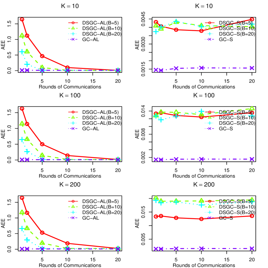
Figure 1: The AEEs versus rounds of communications for Case.1 based on DSGCDMM algorithm against different $B^{\prime}$s, where $\sigma=0.2$. The columns 1—2 are for the results based on different penalties.

To further validate the estimation accuracy of our proposed DSGCDMM algorithm, we compare the AEEs by setting three different values of the maximum number of iterations (denoted as $B$) in Algorithm 2 under different penalty types. Specifically, we consider $B\in\{5,10,20\}$ and five different values of the number of communication rounds, denoted by $L\in\{1,2,5,10,20\}$. Figures 1—2 report the AEEs for Case 1. and Case 2. under different simulation settings.

From the simulation results, we can observe that all the AEEs of DSGC-AL decrease as $L$ increases to 20. Furthermore, we observe that the AEEs at $B=20$ converge rapidly to those of GC-AL, and are smaller than those at $B=5$ and $B=10$. This implies that the proposed approach, DSGCDMM with adaptive LASSO penalty, yields an estimator that performs as well as the global method, GCDMM with adaptive LASSO penalty, as the number of communication rounds approaches infinity. The results shown in the figures intuitively demonstrate that the estimation accuracy of DSGC-AL increases as the number of communication rounds and the maximum number of iterations in Algorithm 2 increase. Furthermore, we observe that the AEEs of DSGC-S are consistently very close to those of GC-S, regardless of the values of $L^{\prime}$s and $B^{\prime}$s. Furthermore, we observe that the AEEs of DSGC-S are significantly smaller than those of DSGC-AL. This is because SCAD-based approaches require the LLA/CD algorithm, which results in our DSGCDMM algorithm with the SCAD penalty type converging quickly. To conclude, the estimator obtained by implementing the DSGCDMM algorithm can achieve comparable performance with the global estimator, provided that an appropriate number of communication rounds and maximum number of iterations are used.

Table 1: Variable selection performance for Case 1. when the penalty function is determined as AL type.

	Number of Machines	Method	FP	FN	FP-C	FP-NC	FN-C	FN-NC
$\sigma=0.2$	$K=10$	DSGC-AL	0.0(0.000)	0(0)	0.00(0.000)	0.00(0.000)	0(0)	0(0)
		DSC-AL	0.0(0.000)	0(0)	0.00(0.000)	0.00(0.000)	0(0)	0(0)
		GC-AL	0.0(0.000)	0(0)	0.00(0.000)	0.00(0.000)	0(0)	0(0)
		AC-AL	0.0(0.000)	0(0)	0.00(0.000)	0.00(0.000)	0(0)	0(0)
	$K=100$	DSGC-AL	0.0(0.000)	0(0)	0.00(0.000)	0.00(0.000)	0(0)	0(0)
		DSC-AL	0.0(0.000)	0(0)	0.00(0.000)	0.00(0.000)	0(0)	0(0)
		GC-AL	0.0(0.000)	0(0)	0.00(0.000)	0.00(0.000)	0(0)	0(0)
		AC-AL	0.2(0.523)	0(0)	0.15(0.489)	0.05(0.224)	0(0)	0(0)
	$K=200$	DSGC-AL	0.0(0.000)	0(0)	0.00(0.000)	0.00(0.000)	0(0)	0(0)
		DSC-AL	0.0(0.000)	0(0)	0.00(0.000)	0.00(0.000)	0(0)	0(0)
		GC-AL	0.0(0.000)	0(0)	0.00(0.000)	0.00(0.000)	0(0)	0(0)
		AC-AL	10.9(1.373)	0(0)	7.40(1.273)	3.50(1.051)	0(0)	0(0)
$\sigma=0.5$	$K=10$	DSGC-AL	0.00(0.000)	0(0)	0.00(0.000)	0.00(0.000)	0(0)	0(0)
		DSC-AL	0.00(0.000)	0(0)	0.00(0.000)	0.00(0.000)	0(0)	0(0)
		GC-AL	0.00(0.000)	0(0)	0.00(0.000)	0.00(0.000)	0(0)	0(0)
		AC-AL	0.00(0.000)	0(0)	0.00(0.000)	0.00(0.000)	0(0)	0(0)
	$K=100$	DSGC-AL	0.00(0.000)	0(0)	0.00(0.000)	0.00(0.000)	0(0)	0(0)
		DSC-AL	0.00(0.000)	0(0)	0.00(0.000)	0.00(0.000)	0(0)	0(0)
		GC-AL	0.00(0.000)	0(0)	0.00(0.000)	0.00(0.000)	0(0)	0(0)
		AC-AL	4.95(6.621)	0(0)	3.25(4.253)	1.70(2.386)	0(0)	0(0)
	$K=200$	DSGC-AL	0.25(0.444)	0(0)	0.20(0.410)	0.05(0.224)	0(0)	0(0)
		DSC-AL	0.00(0.000)	0(0)	0.00(0.000)	0.00(0.000)	0(0)	0(0)
		GC-AL	0.00(0.000)	0(0)	0.00(0.000)	0.00(0.000)	0(0)	0(0)
		AC-AL	12.20(1.765)	0(0)	8.10(0.968)	4.10(0.912)	0(0)	0(0)
Note: The respective standard errors are recorded in the parentheses.

Table 2: Variable selection performance for Case 1. when the penalty function is determined as SCAD type.

	Number of Machines	Method	FP	FN	FP-C	FP-NC	FN-C	FN-NC
$\sigma=0.2$	$K=10$	DSGC-S	0.00(0.000)	0(0)	0.00(0.000)	0.00(0.000)	0(0)	0(0)
		DSC-S	0.00(0.000)	0(0)	0.00(0.000)	0.00(0.000)	0(0)	0(0)
		GC-S	0.00(0.000)	0(0)	0.00(0.000)	0.00(0.000)	0(0)	0(0)
		AC-S	0.00(0.000)	0(0)	0.00(0.000)	0.00(0.000)	0(0)	0(0)
	$K=100$	DSGC-S	0.00(0.000)	0(0)	0.00(0.000)	0.00(0.000)	0(0)	0(0)
		DSC-S	0.00(0.000)	0(0)	0.00(0.000)	0.00(0.000)	0(0)	0(0)
		GC-S	0.00(0.000)	0(0)	0.00(0.000)	0.00(0.000)	0(0)	0(0)
		AC-S	1.75(3.582)	0(0)	1.50(2.911)	0.25(0.910)	0(0)	0(0)
	$K=200$	DSGC-S	0.10(0.447)	0(0)	0.10(0.447)	0.00(0.000)	0(0)	0(0)
		DSC-S	0.00(0.000)	0(0)	0.00(0.000)	0.00(0.000)	0(0)	0(0)
		GC-S	0.00(0.000)	0(0)	0.00(0.000)	0.00(0.000)	0(0)	0(0)
		AC-S	7.40(5.651)	0(0)	5.05(3.649)	2.35(2.183)	0(0)	0(0)
$\sigma=0.5$	$K=10$	DSGC-S	0.00(0.000)	0.00(0.000)	0.00(0.000)	0.0(0.000)	0.00(0.000)	0(0)
		DSC-S	0.00(0.000)	0.05(0.224)	0.00(0.000)	0.0(0.000)	0.05(0.224)	0(0)
		GC-S	0.00(0.000)	0.00(0.000)	0.00(0.000)	0.0(0.000)	0.00(0.000)	0(0)
		AC-S	0.00(0.000)	0.00(0.000)	0.00(0.000)	0.0(0.000)	0.00(0.000)	0(0)
	$K=100$	DSGC-S	0.10(0.308)	0.00(0.000)	0.10(0.308)	0.0(0.000)	0.00(0.000)	0(0)
		DSC-S	0.00(0.000)	0.00(0.000)	0.00(0.000)	0.0(0.000)	0.00(0.000)	0(0)
		GC-S	0.00(0.000)	0.00(0.000)	0.00(0.000)	0.0(0.000)	0.00(0.000)	0(0)
		AC-S	3.55(5.073)	0.00(0.000)	2.65(3.703)	0.9(1.553)	0.00(0.000)	0(0)
	$K=200$	DSGC-S	0.25(0.910)	0.00(0.000)	0.15(0.671)	0.1(0.308)	0.00(0.000)	0(0)
		DSC-S	0.00(0.000)	0.00(0.000)	0.00(0.000)	0.0(0.000)	0.00(0.000)	0(0)
		GC-S	0.00(0.000)	0.00(0.000)	0.00(0.000)	0.0(0.000)	0.00(0.000)	0(0)
		AC-S	7.10(6.069)	0.00(0.000)	4.80(3.847)	2.3(2.342)	0.00(0.000)	0(0)
Note: The respective standard errors are recorded in the parentheses.

Table 3: Variable selection performance for Case 2. when the penalty function is determined as AL type.

	Number of Machines	Method	FP	FN	FP-C	FP-NC	FN-C	FN-NC
$\sigma=0.2$	$K=10$	DSGC-AL	0.00(0.000)	0(0)	0.00(0.000)	0.0(0.000)	0(0)	0(0)
		DSC-AL	0.00(0.000)	0(0)	0.00(0.000)	0.0(0.000)	0(0)	0(0)
		GC-AL	0.00(0.000)	0(0)	0.00(0.000)	0.0(0.000)	0(0)	0(0)
		AC-AL	0.00(0.000)	0(0)	0.00(0.000)	0.0(0.000)	0(0)	0(0)
	$K=100$	DSGC-AL	0.00(0.000)	0(0)	0.00(0.000)	0.0(0.000)	0(0)	0(0)
		DSC-AL	0.00(0.000)	0(0)	0.00(0.000)	0.0(0.000)	0(0)	0(0)
		GC-AL	0.00(0.000)	0(0)	0.00(0.000)	0.0(0.000)	0(0)	0(0)
		AC-AL	0.00(0.000)	0(0)	0.00(0.000)	0.0(0.000)	0(0)	0(0)
	$K=200$	DSGC-AL	0.00(0.000)	0(0)	0.00(0.000)	0.0(0.000)	0(0)	0(0)
		DSC-AL	0.00(0.000)	0(0)	0.00(0.000)	0.0(0.000)	0(0)	0(0)
		GC-AL	0.00(0.000)	0(0)	0.00(0.000)	0.0(0.000)	0(0)	0(0)
		AC-AL	8.05(1.959)	0(0)	5.65(1.531)	2.4(1.046)	0(0)	0(0)
$\sigma=0.5$	$K=10$	DSGC-AL	0.00(0.000)	0(0)	0.00(0.000)	0.00(0.000)	0(0)	0(0)
		DSC-AL	0.00(0.000)	0(0)	0.00(0.000)	0.00(0.000)	0(0)	0(0)
		GC-AL	0.00(0.000)	0(0)	0.00(0.000)	0.00(0.000)	0(0)	0(0)
		AC-AL	0.00(0.000)	0(0)	0.00(0.000)	0.00(0.000)	0(0)	0(0)
	$K=100$	DSGC-AL	0.00(0.000)	0(0)	0.00(0.000)	0.00(0.000)	0(0)	0(0)
		DSC-AL	0.00(0.000)	0(0)	0.00(0.000)	0.00(0.000)	0(0)	0(0)
		GC-AL	0.00(0.000)	0(0)	0.00(0.000)	0.00(0.000)	0(0)	0(0)
		AC-AL	4.95(6.509)	0(0)	3.25(4.241)	1.70(2.296)	0(0)	0(0)
	$K=200$	DSGC-AL	0.15(0.366)	0(0)	0.10(0.308)	0.05(0.224)	0(0)	0(0)
		DSC-AL	0.00(0.000)	0(0)	0.00(0.000)	0.00(0.000)	0(0)	0(0)
		GC-AL	0.00(0.000)	0(0)	0.00(0.000)	0.00(0.000)	0(0)	0(0)
		AC-AL	10.70(2.557)	0(0)	7.40(1.465)	3.30(1.559)	0(0)	0(0)
Note: The respective standard errors are recorded in the parentheses.

Table 4: Variable selection performance for Case 2. when the penalty function is determined as SCAD type.

	Number of Machines	Method	FP	FN	FP-C	FP-NC	FN-C	FN-NC
$\sigma=0.2$	$K=10$	DSGC-S	0.00(0.000)	0(0)	0.00(0.000)	0.00(0.000)	0(0)	0(0)
		DSC-S	0.00(0.000)	0(0)	0.00(0.000)	0.00(0.000)	0(0)	0(0)
		GC-S	0.00(0.000)	0(0)	0.00(0.000)	0.00(0.000)	0(0)	0(0)
		AC-S	0.00(0.000)	0(0)	0.00(0.000)	0.00(0.000)	0(0)	0(0)
	$K=100$	DSGC-S	0.05(0.224)	0(0)	0.05(0.224)	0.00(0.000)	0(0)	0(0)
		DSC-S	0.00(0.000)	0(0)	0.00(0.000)	0.00(0.000)	0(0)	0(0)
		GC-S	0.00(0.000)	0(0)	0.00(0.000)	0.00(0.000)	0(0)	0(0)
		AC-S	2.30(3.988)	0(0)	1.95(3.154)	0.35(0.875)	0(0)	0(0)
	$K=200$	DSGC-S	0.55(0.826)	0(0)	0.40(0.754)	0.15(0.489)	0(0)	0(0)
		DSC-S	0.00(0.000)	0(0)	0.00(0.000)	0.00(0.000)	0(0)	0(0)
		GC-S	0.00(0.000)	0(0)	0.00(0.000)	0.00(0.000)	0(0)	0(0)
		AC-S	7.65(4.891)	0(0)	6.40(3.831)	1.25(1.773)	0(0)	0(0)
$\sigma=0.5$	$K=10$	DSGC-S	0.00(0.000)	0(0)	0.00(0.000)	0.00(0.000)	0(0)	0(0)
		DSC-S	0.00(0.000)	0(0)	0.00(0.000)	0.00(0.000)	0(0)	0(0)
		GC-S	0.00(0.000)	0(0)	0.00(0.000)	0.00(0.000)	0(0)	0(0)
		AC-S	0.00(0.000)	0(0)	0.00(0.000)	0.00(0.000)	0(0)	0(0)
	$K=100$	DSGC-S	0.00(0.000)	0(0)	0.00(0.000)	0.00(0.000)	0(0)	0(0)
		DSC-S	0.00(0.000)	0(0)	0.00(0.000)	0.00(0.000)	0(0)	0(0)
		GC-S	0.00(0.000)	0(0)	0.00(0.000)	0.00(0.000)	0(0)	0(0)
		AC-S	1.30(2.494)	0(0)	1.25(2.314)	0.05(0.224)	0(0)	0(0)
	$K=200$	DSGC-S	0.75(1.251)	0(0)	0.60(1.046)	0.15(0.489)	0(0)	0(0)
		DSC-S	0.00(0.000)	0(0)	0.00(0.000)	0.00(0.000)	0(0)	0(0)
		GC-S	0.00(0.000)	0(0)	0.00(0.000)	0.00(0.000)	0(0)	0(0)
		AC-S	7.95(4.273)	0(0)	6.95(3.486)	1.00(1.556)	0(0)	0(0)
Note: The respective standard errors are recorded in the parentheses.

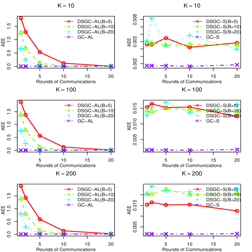
Figure 2: The AEEs versus rounds of communications for Case.1 based on DSGCDMM algorithm against different $B^{\prime}$s, where $\sigma=0.5$. The columns 1—2 are for the results based on different penalties.

5.2 Real Data

The medical insurance(MI) dataset for major chest surgeries contains information about patients who underwent major chest surgery at a large tertiary hospital in Sichuan Province, China, from January 2020 to December 2020. MI dataset is collected by Comprehensive Hospital of a Class-3 Grade-A Hospital in Chengdu, China, and available with reasonable request. The patients were grouped according to the Chinese Diagnosis Related Groups (CHS-DRG) standard for diagnosis and treatment under the National Medical Insurance scheme. Our objective is to predict the medical insurance reimbursement ratio(MIRR) for patients. The MIRR is defined as the ratio of the reimbursement amount(RA) to the total hospitalization costs(THC). After eliminating any values that are not available for RA and THC, the total sample size of MI dataset is $n=37342$. We define hospitalization costs as the explanatory variable, which is composed of $p=15$ components: income from western medicine (IWM), income from diagnosis (ID), income from examination (IE), income from radiology (IR), income from treatment (IT), income from surgery (IS), income from laboratory tests (ILT), income from nursing (IN), income from bed occupancy (IBO), income from medical supplies (IMS), income from Chinese patent medicine (ICP), income from Chinese herbal medicine (ICHM), income from nutrition and meals (INM), income from blood products (IBP), and income from oxygen supplies (IOS). We exclude variables that are not related to treatment costs, such as patient age, medical insurance type, admitting department, and discharge department. Additionally, we add $q=20$ non-compositional variables $\boldsymbol{V}=(V_{1},\dots,V_{20})\in\mathbbm{R}^{n\times q}$ that are not related to the MIRR, where $\boldsymbol{V}$ is generated from a multivariate $t$ distribution $\boldsymbol{T}_{3}(\boldsymbol{0},\boldsymbol{\Sigma})$ with $3$ degrees of freedom and $\boldsymbol{\Sigma}=(\sigma^{(i\neq j)})$ with $\sigma\in\{0.2,0.5\}$.

In this subsection, because the true parameter is unknown and the computing procedure is carried on a single machine, we first evaluate the prediction accuracy of our proposed methods DSCDMM and DSGCDMM, and compare them with GCDMM and ACDMM proposed in Section 5.1. The penalty function is specified as adaptive LASSO and SCAD. We artificially split the PTS data set into $K=\{10,20,50\}$ subdata sets, and the other simulation settings are same as those in Section 5.1. To obtain stable and reliable prediction results, we execute the 5-folds cross-validation(CV) to evaluate the performance. More specifically, the CV prediction error is measured by the $\ell_{q}$ losses, i.e.,

$$\text{CVL}_{q}=\frac{1}{5}\sum_{l=1}^{5}\frac{\|\boldsymbol{y}_{v_{l}}-\boldsymbol{\Pi}_{v_{l}}\widehat{\boldsymbol{\zeta}}_{l}\|_{q}}{n_{v_{l}}}$$

with $q=1,2,\infty$, where $\{\boldsymbol{y}_{v_{l}},\boldsymbol{\Pi}_{v_{l}}\}$ is the validation dataset for $l^{th}$ fold and $n_{v_{l}}$ is its sample size, $\widehat{\boldsymbol{\zeta}}_{l}$ is obtained by fitting the training datasets for $l^{th}$ fold. We also calculate the average values of FN-NC and FP-NC(as defined in Section 5.1), which are relabeled as CVFN-NC and CVFP-NC, respectively, by using the training dataset for each fold in the CV procedure. This allows us to validate the accuracy of variable selection. Tables 5—6 present the average values of three metrics, namely, $\text{CVL}_{q}$, CVFN-NC, and CVFP-NC, based on 100 simulations for $\sigma=0.2$ and $\sigma=0.5$, respectively. By examining the tables for different values of $\sigma$ and $K$, we observe that the values of $\text{CVL}_{q}$ for DSGCDMM and DSCDMM, with both adaptive LASSO and SCAD penalties, are extremely close to those of the global method GCDMM and the average-based method ACDMM. Additionally, we note that the values of CVFP-NC for ACDMM become increasingly larger than those of other two distributed methods DSGCDMM and DSCDMM as the number of machines increases. This suggests that average-based methods with only one round of communication exhibit lower statistical efficiency when the number of machines is large. Besides, although the values of DSGCDMM also increase as the number of machines increases, DSGCDMM has more stable and much smaller CVFP-NC compared to ACDMM. We can draw a conclusion that our proposed DSGCDMM and DSCDMM have good prediction performance and demonstrates its practicality and effectiveness for handling real-world data. It is noted that DSGCDMM and DSCDMM have different applicable scenarios, namely centralized and decentralized frameworks. Users can choose the appropriate method based on the specific scenario.

Table 5: The simulation results for the MI data over 100 replications, where $\sigma=0.2$.

	Method	$\text{CVL}_{1}$	$\text{CVL}_{2}$	$\text{CVL}_{\infty}$	CVFP-NC	CVFN-NC
$K=10$	DSGC-AL	$0.28076$	$0.00449$	$0.00016$	$0$	$0$
	DSC-AL	$0.30293$	$0.00480$	$0.00016$	$0$	$0$
	GC-AL	$0.27161$	$0.00433$	$0.00019$	$0$	$0$
	AC-AL	$0.27321$	$0.00436$	$0.00016$	$0$	$0$
	DSGC-S	$0.26604$	$0.00427$	$0.00019$	$0.43$	$0$
	DSC-S	$0.31042$	$0.00489$	$0.00020$	$0$	$0$
	GC-S	$0.26385$	$0.00424$	$0.00028$	$0$	$0$
	AC-S	$0.26323$	$0.00423$	$0.00020$	$2.87$	$0$
$K=20$	DSGC-AL	$0.28190$	$0.00450$	$0.00016$	$0$	$0$
	DSC-AL	$0.30178$	$0.00479$	$0.00016$	$0$	$0$
	GC-AL	$0.27164$	$0.00433$	$0.00019$	$0$	$0$
	AC-AL	$0.26560$	$0.00426$	$0.00020$	$0$	$0$
	DSGC-S	$0.26590$	$0.00425$	$0.00019$	$1.32$	$0$
	DSC-S	$0.30535$	$0.00486$	$0.00016$	$0$	$0$
	GC-S	$0.26381$	$0.00424$	$0.00028$	$0$	$0$
	AC-S	$0.26489$	$0.00432$	$0.00048$	$13.21$	$0$
$K=50$	DSGC-AL	$0.27966$	$0.00447$	$0.00016$	$0$	$0$
	DSC-AL	$0.15684$	$0.00255$	$0.00010$	$0$	$0$
	GC-AL	$0.27162$	$0.00433$	$0.00019$	$0$	$0$
	AC-AL	$0.25711$	$0.00414$	$0.00019$	$10.05$	$0$
	DSGC-S	$0.27341$	$0.00437$	$0.00025$	$3.99$	$0$
	DSC-S	$0.30150$	$0.00478$	$0.00016$	$0$	$0$
	GC-S	$0.26385$	$0.00424$	$0.00028$	$0$	$0$
	AC-S	$0.25260$	$0.00409$	$0.00025$	$19.32$	$0$

Table 6: The simulation results for the MI data over 100 replications, where $\sigma=0.5$.

	Method	$\text{CVL}_{1}$	$\text{CVL}_{2}$	$\text{CVL}_{\infty}$	CVFP-NC	CVFN-NC
$K=10$	DSGC-AL	$0.28083$	$0.00449$	$0.00016$	$0$	$0$
	DSC-AL	$0.30314$	$0.00480$	$0.00016$	$0$	$0$
	GC-AL	$0.27151$	$0.00433$	$0.00019$	$0$	$0$
	AC-AL	$0.27322$	$0.00436$	$0.00016$	$0$	$0$
	DSGC-S	$0.26603$	$0.00427$	$0.00019$	$0.33$	$0$
	DSC-S	$0.31037$	$0.00489$	$0.00020$	$0$	$0$
	GC-S	$0.26381$	$0.00424$	$0.00028$	$0$	$0$
	AC-S	$0.26259$	$0.00422$	$0.00021$	$3.13$	$0$
$K=20$	DSGC-AL	$0.28192$	$0.00450$	$0.00016$	$0$	$0$
	DSC-AL	$0.30180$	$0.00479$	$0.00016$	$0$	$0$
	GC-AL	$0.27158$	$0.00433$	$0.00019$	$0$	$0$
	AC-AL	$0.26561$	$0.00426$	$0.00020$	$0.04$	$0$
	DSGC-S	$0.26901$	$0.00430$	$0.00020$	$1.39$	$0$
	DSC-S	$0.30203$	$0.00482$	$0.00016$	$0$	$0$
	GC-S	$0.26353$	$0.00424$	$0.00028$	$0$	$0$
	AC-S	$0.26464$	$0.00432$	$0.00048$	$12.79$	$0$
$K=50$	DSGC-AL	$0.27977$	$0.00447$	$0.00016$	$0$	$0$
	DSC-AL	$0.15698$	$0.00256$	$0.00010$	$0$	$0$
	GC-AL	$0.27160$	$0.00433$	$0.00019$	$0$	$0$
	AC-AL	$0.25763$	$0.00415$	$0.00019$	$11.85$	$0$
	DSGC-S	$0.27306$	$0.00437$	$0.00026$	$3.75$	$0$
	DSC-S	$0.30177$	$0.00479$	$0.00016$	$0$	$0$
	GC-S	$0.26385$	$0.00424$	$0.00028$	$0$	$0$
	AC-S	$0.25268$	$0.00409$	$0.00025$	$19$	$0$

6 Concluding Remarks

In this paper, we propose variable selection procedures for the distributed massive linear regression with compositional covariates, and we consider two distributed frameworks with centralized and decentralized topologies. In the centralized manner, by combining ADMM(Boyd et al. (2011)) and CDMM(Lin et al. (2014)) algorithms, we solve the distributed optimization problem with two types of constraints that are related to the global model parameter. We also present the associated statistical efficient algorithm, named DSCDMM. To address the drawbacks of the centralized distributed system, we further propose a novel decentralized approach, namely DSGCDMM, which is motivated from the GADMM algorithm(Elgabli et al. (2020a)). The DSGCDMM algorithm can solve the distributed constrained optimization problem that is only related to the local machine parameters. Simulation studies and a real data example demonstrate that our proposed DSCDMM and DSGCDMM algorithms can exhibit their statistical efficiency in variable selection procedures under centralized and decentralized manners. In summary, both of these two algorithms have their own applicable scenarios in practice.

However, this work has several limitations. First, the DSCDMM and DSGCDMM algorithms perform less computational efficiency according to the running times. Second, in the high-dimensional or ultra high-dimensional settings, our proposed approaches may not work well, particularly when there is a high computational burden due to multiple rounds of communication and the relatively low computational efficiency of coordinate-wise descent algorithms. Especially, for problems with a large number of variables, coordinate-wise descent algorithms can be very inefficient. This is because they require evaluating the objective function and its gradient at each iteration, which can be very computationally expensive for large problems(Wright (2015)). In addition, the heterogeneity for the distributed datasets from machine to machine and privacy-preserving issues in both distributed learning and federated learning(Konečnỳ et al. (2016); Kairouz et al. (2021)) are not considered in our framework(Duan et al. (2022); Zhu et al. (2021)). Therefore, developing a more fast and communication-efficient methodology together with efficient statistical estimation and computation under the above issues is our next objective for next work. Moreover, there are many interesting and valuable research opportunities in the field of decentralized distributed machine learning that are worth pursuing in the future.

Acknowledgments and Disclosure of Funding

Ma’s research was fully supported by the National Natural Science Foundation of China (Grant No.12101439) and the Natural Science Foundation of Jiangsu Province (Grant No.BK20200854). Huang’s research was fully supported by the Sichuan Natural Science Foundation (Grant No.2022NSFSC1850), the New Interdisciplinary Training Fund(Grant No.2682023JX004), and partially supported by National Natural Science Foundation of China(Grant No.72033002).

Appendix A

Proof of Lemma 1 It is noted that the augmented Lagrangian function $\mathscr{L}_{\rho}$ in (15) is sub-differentiable. Under the proofs of Elgabli et al. (2020a), for the minimizers $\boldsymbol{\zeta}^{l+1}_{k}$’s with $k\in\mathscr{N}_{h}$ of (16) ans (17), the expressions (35) and (36) can be rewritten as

$$\boldsymbol{0}\in\partial\mathbb{Q}_{k}(\boldsymbol{\zeta}_{k}^{l+1})+\mu_{k}^{l+1}\boldsymbol{C}+\boldsymbol{\gamma}_{k}^{l+1}+\boldsymbol{s}_{k}^{l+1},\leavevmode\nobreak\ k=1.$$ (44)

$$\boldsymbol{0}\in\partial\mathbb{Q}_{k}(\boldsymbol{\zeta}_{k}^{l+1})+\mu_{k}^{l+1}\boldsymbol{C}-\boldsymbol{\gamma}_{k-1}^{l+1}+\boldsymbol{\gamma}_{k}^{l+1}+\boldsymbol{s}_{k}^{l+1},\leavevmode\nobreak\ k\in\mathscr{N}_{h}\backslash\{1\}.$$ (45)

Following the technical proof of Lemma 1 in Elgabli et al. (2020a), we also denote $\boldsymbol{\gamma}_{0}^{l+1}=\boldsymbol{\gamma}_{K}^{l+1}=\boldsymbol{0}$ for simplicity. It is observed that $\boldsymbol{\zeta}_{k\in\mathscr{N}_{h}}^{l+1}$ and $\boldsymbol{\zeta}_{k\in\mathscr{N}_{t}}^{l+1}$ can be regarded as the minimizers of the following two convex objective functions $\mathbb{H}_{k}(\boldsymbol{\zeta}_{k})$ and $\mathbb{T}_{k}(\boldsymbol{\zeta}_{k})$, respectively. They are separately defined as

$$\mathbb{H}_{k}(\boldsymbol{\zeta}_{k}):=\mathbb{Q}_{k}(\boldsymbol{\zeta}_{k})+\left\langle\mu_{k}^{l+1}\boldsymbol{C}-\boldsymbol{\gamma}_{k-1}^{l+1}+\boldsymbol{\gamma}_{k}^{l+1}+\boldsymbol{s}_{k}^{l+1},\boldsymbol{\zeta}_{k}\right\rangle,$$ (46)

and

$$\mathbb{T}_{k}(\boldsymbol{\zeta}_{k}):=\mathbb{Q}_{k}(\boldsymbol{\zeta}_{k})+\left\langle\mu_{k}^{l+1}\boldsymbol{C}-\boldsymbol{\gamma}_{k-1}^{l+1}+\boldsymbol{\gamma}_{k}^{l+1},\boldsymbol{\zeta}_{k}\right\rangle.$$ (47)

Thus, for the optimal solution $\boldsymbol{\zeta}^{\star}$ of the problem in (14), we can obtain

$$\mathbb{H}_{k}(\boldsymbol{\zeta}_{k}^{l+1}) \leq\mathbb{H}_{k}(\boldsymbol{\zeta}_{k}^{\star}),$$ (48)

$$\mathbb{T}_{k}(\boldsymbol{\zeta}_{k}^{l+1}) \leq\mathbb{T}_{k}(\boldsymbol{\zeta}_{k}^{\star}).$$ (49)

It follows that

$$\begin{split}&\sum_{k\in\mathscr{N}_{h}}\mathbb{H}_{k}(\boldsymbol{\zeta}_{k}^{l+1})+\sum_{k\in\mathscr{N}_{t}}\mathbb{T}_{k}(\boldsymbol{\zeta}_{k}^{l+1})\leq\sum_{k\in\mathscr{N}_{h}}\mathbb{H}_{k}(\boldsymbol{\zeta}_{k}^{\star})+\sum_{k\in\mathscr{N}_{t}}\mathbb{T}_{k}(\boldsymbol{\zeta}_{k}^{\star}),\end{split}$$ (50)

After rearranging the terms and substituting the expression from (46) and (47), (50) can be re-expressed as

$$\begin{split}&\sum_{k=1}^{K}\mathbb{Q}_{k}(\boldsymbol{\zeta}_{k}^{l+1})-\sum_{k=1}^{K}\mathbb{Q}_{k}(\boldsymbol{\zeta}_{k}^{\star})\\ &\leq\sum_{k=1}^{K}\left\langle\mu_{k}^{l+1}\boldsymbol{C},\boldsymbol{\zeta}_{k}^{\star}\right\rangle-\sum_{k=1}^{K}\left\langle\mu_{k}^{l+1}\boldsymbol{C},\boldsymbol{\zeta}_{k}^{l+1}\right\rangle+\sum_{k\in\mathscr{N}_{t}}\left\langle-\boldsymbol{\gamma}_{k-1}^{l+1}+\boldsymbol{\gamma}_{k}^{l+1},\boldsymbol{\zeta}^{\star}\right\rangle+\sum_{k\in\mathscr{N}_{h}}\left\langle-\boldsymbol{\gamma}_{k-1}^{l+1}+\boldsymbol{\gamma}_{k}^{l+1},\boldsymbol{\zeta}^{\star}\right\rangle\\ &-\sum_{k\in\mathscr{N}_{t}}\left\langle-\boldsymbol{\gamma}_{k-1}^{l+1}+\boldsymbol{\gamma}_{k}^{l+1},\boldsymbol{\zeta}_{k}^{l+1}\right\rangle-\sum_{k\in\mathscr{N}_{h}}\left\langle-\boldsymbol{\gamma}_{k-1}^{l+1}+\boldsymbol{\gamma}_{k}^{l+1},\boldsymbol{\zeta}_{k}^{l+1}\right\rangle+\sum_{k\in\mathscr{N}_{h}}\left\langle\boldsymbol{s}_{k}^{l+1},\boldsymbol{\zeta}^{\star}-\boldsymbol{\zeta}^{l+1}_{k}\right\rangle.\end{split}$$ (51)

Through the proof of Lemma 1 in Elgabli et al. (2020a) and the fact $\boldsymbol{C}^{\top}\boldsymbol{\zeta}^{\star}_{k}=0$, we have

$$\sum_{k\in\mathscr{N}_{t}}\left\langle-\boldsymbol{\gamma}_{k-1}^{l+1}+\boldsymbol{\gamma}_{k}^{l+1},\boldsymbol{\zeta}^{\star}\right\rangle+\sum_{k\in\mathscr{N}_{h}}\left\langle-\boldsymbol{\gamma}_{k-1}^{l+1}+\boldsymbol{\gamma}_{k}^{l+1},\boldsymbol{\zeta}^{\star}\right\rangle=0,$$

$$\sum_{k\in\mathscr{N}_{t}}\left\langle-\boldsymbol{\gamma}_{k-1}^{l+1}+\boldsymbol{\gamma}_{k}^{l+1},\boldsymbol{\zeta}_{k}^{l+1}\right\rangle+\sum_{k\in\mathscr{N}_{h}}\left\langle-\boldsymbol{\gamma}_{k-1}^{l+1}+\boldsymbol{\gamma}_{k}^{l+1},\boldsymbol{\zeta}_{k}^{l+1}\right\rangle=\sum_{k=1}^{K-1}\left\langle\boldsymbol{\gamma}_{k}^{l+1},\boldsymbol{r}_{k}^{l+1}\right\rangle.$$

Therefore, we can obtain

$$\begin{split}\sum_{k=1}^{K}\mathbb{Q}_{k}(\boldsymbol{\zeta}_{k}^{l+1})-\sum_{k=1}^{K}\mathbb{Q}_{k}(\boldsymbol{\zeta}_{k}^{\star})&\leq-\sum_{k=1}^{K}\left\langle\mu_{k}^{l+1}\boldsymbol{C},\boldsymbol{\zeta}_{k}^{l+1}\right\rangle-\sum_{k=1}^{K-1}\left\langle\boldsymbol{\gamma}_{k}^{l+1},\boldsymbol{r}_{k}^{l+1}\right\rangle+\sum_{k\in\mathscr{N}_{h}}\left\langle\boldsymbol{s}_{k}^{l+1},\boldsymbol{\zeta}^{\star}-\boldsymbol{\zeta}^{l+1}_{k}\right\rangle\\ &=-\sum_{k=1}^{K}\mu_{k}^{l+1}g_{k}^{l+1}-\sum_{k=1}^{K-1}\left\langle\boldsymbol{\gamma}_{k}^{l+1},\boldsymbol{r}_{k}^{l+1}\right\rangle+\sum_{k\in\mathscr{N}_{h}}\left\langle\boldsymbol{s}_{k}^{l+1},\boldsymbol{\zeta}^{\star}-\boldsymbol{\zeta}^{l+1}_{k}\right\rangle.\end{split}$$ (52)

According to the proof steps of Boyd et al. (2011); Giesen and Laue (2016); Elgabli et al. (2020a), for a saddle point $(\boldsymbol{\zeta}^{\star},\{\mu_{k}^{\star}\}_{k=1}^{K},\{\boldsymbol{\gamma}_{k}^{\star}\}_{k=1}^{K})$ of $\mathscr{L}_{0}\left(\{\boldsymbol{\zeta}_{k}\}^{K}_{k=1},\{\mu_{k}\}_{k=1}^{K},\{\boldsymbol{\gamma}_{k}\}_{k=1}^{K}\right)$, the following inequality holds:

$$\mathscr{L}_{0}\left(\boldsymbol{\zeta}^{\star},\{\mu_{k}^{\star}\}_{k=1}^{K},\{\boldsymbol{\gamma}_{k}^{\star}\}_{k=1}^{K}\right)\leq\mathscr{L}_{0}\left(\{\boldsymbol{\zeta}_{k}^{l+1}\}^{K}_{k=1},\{\mu_{k}^{\star}\}_{k=1}^{K},\{\boldsymbol{\gamma}_{k}^{\star}\}_{k=1}^{K}\right).$$ (53)

Using the expression for the augmented Lagrangian as given in equation (15) to substitute on both sides of equation (53), it follows that

$$\begin{split}\sum_{k=1}^{K}\left(\mathbb{Q}_{k}(\boldsymbol{\zeta}_{k}^{l+1})-\mathbb{Q}_{k}(\boldsymbol{\zeta}_{k}^{\star})\right)&\geq-\sum_{k=1}^{K}\left\langle\mu_{k}^{\star}\boldsymbol{C}^{\top},\boldsymbol{\zeta}_{k}^{l+1}\right\rangle-\sum_{k=1}^{K-1}\left\langle\boldsymbol{\gamma}_{k}^{\star},\boldsymbol{r}_{k}^{l+1}\right\rangle\\ &=-\sum_{k=1}^{K}\mu_{k}^{\star}g_{k}^{l+1}-\sum_{k=1}^{K-1}\left\langle\boldsymbol{\gamma}_{k}^{\star},\boldsymbol{r}_{k}^{l+1}\right\rangle.\end{split}$$ (54)

This completes the proof of the lemma.  

Appendix B

Proof of Theorem 4.1. Our procedures of proof likewise follow the steps of Boyd et al. (2011); Elgabli et al. (2020a). From Lemma 1, we can obtain

$$-\sum_{k=1}^{K}\mu_{k}^{\star}g_{k}^{l+1}-\sum_{k=1}^{K-1}\left\langle\boldsymbol{\gamma}_{k}^{\star},\boldsymbol{r}_{k}^{l+1}\right\rangle\leq-\sum_{k=1}^{K}\mu_{k}^{l+1}g_{k}^{l+1}-\sum_{k=1}^{K-1}\left\langle\boldsymbol{\gamma}_{k}^{l+1},\boldsymbol{r}_{k}^{l+1}\right\rangle+\sum_{k\in\mathscr{N}_{h}}\left\langle\boldsymbol{s}^{l+1}_{k},\boldsymbol{\zeta}_{k}^{\star}-\boldsymbol{\zeta}_{k}^{l+1}\right\rangle.$$ (55)

After rearranging (55) and multiplying both sides of (55) by $2$, we have

$$\begin{split}&2\sum_{k=1}^{K}(\mu_{k}^{l+1}-\mu_{k}^{\star})g_{k}^{l+1}+2\sum_{k=1}^{K-1}\left\langle\boldsymbol{\gamma}_{k}^{l+1}-\boldsymbol{\gamma}_{k}^{\star},\boldsymbol{r}_{k}^{l+1}\right\rangle+2\sum_{k\in\mathscr{N}_{h}}\left\langle\boldsymbol{s}_{k}^{l+1},\boldsymbol{\zeta}_{k}^{l+1}-\boldsymbol{\zeta}_{k}^{\star}\right\rangle\leq 0.\end{split}$$ (56)

The update of dual variable $\mu_{k}^{l+1}$ in (20) can be rewritten as $\mu_{k}^{l+1}=\mu_{k}^{l}+\rho g_{k}^{l+1}$. Then $g_{k}^{l+1}=(\mu_{k}^{l+1}-\mu_{k}^{l})/\rho$. Besides,

$$\mu_{k}^{l+1}-\mu_{k}^{l}=(\mu_{k}^{l+1}-\mu_{k}^{\star})-(\mu_{k}^{l}-\mu_{k}^{\star}).$$

Direct calculation yields

$$\begin{split}2\sum_{k=1}^{K}(\mu_{k}^{l+1}-\mu_{k}^{\star})g_{k}^{l+1}&=2\sum_{k=1}^{K}(\mu_{k}^{l}+\rho g_{k}^{l+1}-\mu_{k}^{\star})g_{k}^{l+1}\\ &=2\sum_{k=1}^{K}(\mu_{k}^{l}-\mu_{k}^{\star})g_{k}^{l+1}+\rho\sum_{k=1}^{K}(g_{k}^{l+1})^{2}+\rho\sum_{k=1}^{K}(g_{k}^{l+1})^{2}\\ &=\frac{2}{\rho}\sum_{k=1}^{K}(\mu_{k}^{l}-\mu_{k}^{\star})(\mu_{k}^{l+1}-\mu_{k}^{l})+\frac{1}{\rho}\sum_{k=1}^{K}(\mu_{k}^{l+1}-\mu_{k}^{l})^{2}+\rho\sum_{k=1}^{K}(g_{k}^{l+1})^{2}\\ &=\frac{1}{\rho}\sum_{k=1}^{K}(\mu_{k}^{l+1}-\mu_{k}^{\star})^{2}-\frac{1}{\rho}\sum_{k=1}^{K}(\mu_{k}^{l}-\mu_{k}^{\star})^{2}+\rho\sum_{k=1}^{K}(g^{l+1}_{k})^{2}\\ &:=A_{1}.\end{split}$$ (57)

Applying the similar proof technique as in (57), it holds that

$$\begin{split}2\sum_{k=1}^{K-1}\left\langle\boldsymbol{\gamma}_{k}^{l+1}-\boldsymbol{\gamma}_{k}^{\star},\boldsymbol{r}_{k}^{l+1}\right\rangle&=\frac{1}{\rho}\sum_{k=1}^{K-1}\left\|\boldsymbol{\gamma}_{k}^{l+1}-\boldsymbol{\gamma}_{k}^{\star}\right\|^{2}-\frac{1}{\rho}\sum_{k=1}^{K-1}\left\|\boldsymbol{\gamma}_{k}^{l+1}-\boldsymbol{\gamma}_{k}^{\star}\right\|^{2}+\rho\sum_{k=1}^{K-1}\left\|\boldsymbol{r}_{k}^{l+1}\right\|^{2}\\ &:=A_{2}.\end{split}$$ (58)

Next, following the proof of Theorem 2 in Elgabli et al. (2020a), we have

$$\begin{split}&\leavevmode\nobreak\ 2\sum_{k\in\mathscr{N}_{h}}\left\langle\boldsymbol{s}_{k}^{l+1},\boldsymbol{\zeta}_{k}^{l+1}-\boldsymbol{\zeta}_{k}^{\star}\right\rangle\\ &=\sum_{n\in{\mathscr{N}}_{h}\setminus\{1\}}\left(\begin{array}[]{l}-2\rho\left\langle\boldsymbol{\zeta}_{k-1}^{l+1}-\boldsymbol{\zeta}_{k-1}^{l},\boldsymbol{r}_{k-1}^{l+1}\right\rangle+\rho\left\|\boldsymbol{\zeta}_{k-1}^{l+1}-\boldsymbol{\zeta}_{k-1}^{l}\right\|^{2}+\rho\left\|\boldsymbol{\zeta}^{l+1}_{k-1}-\boldsymbol{\zeta}_{k-1}^{l}\right\|^{2}\\ \leavevmode\nobreak\ \leavevmode\nobreak\ \leavevmode\nobreak\ \leavevmode\nobreak\ \leavevmode\nobreak\ \leavevmode\nobreak\ \leavevmode\nobreak\ \leavevmode\nobreak\ +\rho\left\|\boldsymbol{\zeta}_{k-1}^{l+1}-\boldsymbol{\zeta}^{\star}\right\|^{2}-\rho\left\|\boldsymbol{\zeta}^{l}_{k-1}-\boldsymbol{\zeta}^{\star}\right\|^{2}\end{array}\right)\\ &\leavevmode\nobreak\ \leavevmode\nobreak\ \leavevmode\nobreak\ +\sum\limits_{n\in\mathscr{N}_{h}}\left(2\rho\left\langle\boldsymbol{\zeta}_{k+1}^{l+1}-\boldsymbol{\zeta}_{k+1}^{l},\boldsymbol{r}_{k}^{l+1}\right\rangle+\rho\left\|\boldsymbol{\zeta}_{k+1}^{l+1}-\boldsymbol{\zeta}_{k+1}^{l}\right\|^{2}+\rho\left\|\boldsymbol{\zeta}_{k+1}^{l+1}-\boldsymbol{\zeta}^{\star}\right\|^{2}-\rho\left\|\boldsymbol{\zeta}^{l}_{k+1}-\boldsymbol{\zeta}^{\star}\right\|^{2}\right)\\ &:=A_{3}.\end{split}$$ (59)

Now we define a Lyapunov function $V^{l}$ for our algorithm as

$$V^{l}=\frac{1}{\rho}\sum_{k=1}^{K}(\mu_{k}^{l}-\mu_{k}^{\star})^{2}+\frac{1}{\rho}\sum_{k=1}^{K-1}\left\|\boldsymbol{\gamma}_{k}^{l}-\boldsymbol{\gamma}_{k}^{\star}\right\|^{2}+\rho\sum_{k\in\mathscr{N}_{h}\setminus\{1\}}\left\|\boldsymbol{\zeta}_{k-1}^{l}-\boldsymbol{\zeta}^{\star}\right\|^{2}+\rho\sum_{k\in\mathscr{N}_{h}}\left\|\boldsymbol{\zeta}_{k+1}^{l}-\boldsymbol{\zeta}^{\star}\right\|^{2}.$$ (60)

After rearranging the terms in inequality $A_{1}+A_{2}+A_{3}\geq 0$ and through (60), the following inequality holds

$$\begin{split}V^{l}-V^{l+1}&\geq\rho\sum_{k=1}^{K}(g_{k}^{l+1})^{2}+\rho\sum_{k=1}^{K-1}\left\|\boldsymbol{r}_{k}^{l+1}\right\|^{2}+\Lambda^{l},\end{split}$$ (61)

where

$$\begin{split}\Lambda^{l}&=\left[\rho\sum_{k\in\mathscr{N}_{h}\setminus\{1\}}\left\|\boldsymbol{\zeta}^{l+1}_{k-1}-\boldsymbol{\zeta}_{k-1}^{l}\right\|^{2}+\rho\sum_{k\in\mathscr{N}_{h}}\left\|\boldsymbol{\zeta}_{k+1}^{l+1}-\boldsymbol{\zeta}_{k+1}^{l}\right\|^{2}\right]\\ &\leavevmode\nobreak\ \leavevmode\nobreak\ \leavevmode\nobreak\ \leavevmode\nobreak\ +\left[-2\rho\sum_{n\in\mathscr{N}_{h}\setminus\{1\}}\left\langle\boldsymbol{\zeta}_{k-1}^{l+1}-\boldsymbol{\zeta}_{k-1}^{l},\boldsymbol{r}_{k-1}^{l+1}\right\rangle+2\rho\sum_{k\in\mathscr{N}_{h}}\left\langle\boldsymbol{\zeta}_{k+1}^{l+1}-\boldsymbol{\zeta}_{k+1}^{l},\boldsymbol{r}_{k}^{l+1}\right\rangle\right]\\ &:=\Lambda_{1}^{l}+\Lambda_{2}^{l}.\end{split}$$ (62)

This indicates that $V_{l}$ decreases monotonically at each iteration as long as $\Lambda_{1}^{l}$,$\Lambda_{2}^{l}$ in (62) are positive. It is obvious that $\Lambda_{1}>0$. Applying the proof results directly of Theorem 2 in Elgabli et al. (2020a), we obtain $\Lambda_{2}>0$ holds. Then,

$$\begin{split}V^{l}-V^{l+1}&\geq\rho\sum_{k=1}^{K}(g_{k}^{l+1})^{2}+\rho\sum_{k=1}^{K-1}\left\|\boldsymbol{r}_{k}^{l+1}\right\|^{2}+\Lambda_{1}^{l}.\end{split}$$ (63)

For $l=0,\ldots,L$, $V^{L}\leq V^{0}$ due to the monotonicity decreasing of $V^{l}$. Sum both sides of (63) over $l$, we have

$$\sum_{l=0}^{L}\left[\rho\sum_{k=1}^{K}(g_{k}^{l+1})^{2}+\rho\sum_{k=1}^{K-1}\left\|\boldsymbol{r}_{k}^{l+1}\right\|^{2}+\Lambda_{1}^{l}\right]\leq V^{0}-V^{L}\leq V^{0}.$$ (64)

There is a fact that a series of positive terms that is bounded converges. We infer that the series in the left side of (64) converges as $L\to\infty$. Hence, $g_{k}^{l+1}\to 0$ for all $k=1,\ldots,K$ and $r_{k}^{l+1}\to\boldsymbol{0}$ for all $k=1,\ldots,K-1$, as $l\to\infty$. This completes the proof of propositions 1. and 2. in Theorem 4.1. Furthermore, the fact that $\left\|\boldsymbol{\zeta}^{l+1}_{k-1}-\boldsymbol{\zeta}_{k-1}^{l}\right\|\to 0$ and $\left\|\boldsymbol{\zeta}_{k+1}^{l+1}-\boldsymbol{\zeta}_{k+1}^{l}\right\|\to 0$ as $l\to\infty$ results in $\boldsymbol{s}_{k}^{l}\to\boldsymbol{0}$. This completes the proof of proposition 3. in Theorem 4.1. By the Lemma 1, the propositions 1., 2., 3. in Theorem 4.1 and Squeeze theorem in Sohrab (2003), it holds that, as $l\to\infty$,

$$\sum_{k=1}^{K}\left(\mathbb{Q}_{k}(\boldsymbol{\zeta}_{k}^{l})-\mathbb{Q}_{k}(\boldsymbol{\zeta}_{k}^{\star})\right)\rightarrow 0.$$

This completes the proof of the theorem.

References

- Aitchison (1982) John Aitchison. The statistical analysis of compositional data. Journal of the Royal Statistical Society: Series B (Satistical Methodology), 44(2):139–160, 1982.
- Aitchison and Bacon-Shone (1984) John Aitchison and John Bacon-Shone. Log contrast models for experiments with mixtures. Biometrika, 71(2):323–330, 1984.
- Alenazi (2021) Abdulaziz Alenazi. A review of compositional data analysis and recent advances. Communications in Statistics-Theory and Methods, pages 1–33, 2021.
- Atallah et al. (2022) Elie Atallah, Nazanin Rahnavard, and Qiyu Sun. CoDGraD: A code-based distributed gradient descent scheme for decentralized convex optimization. arXiv preprint arXiv:2204.06344, 2022.
- Boyd et al. (2011) Stephen Boyd, Neal Parikh, Eric Chu, Borja Peleato, Jonathan Eckstein, et al. Distributed optimization and statistical learning via the alternating direction method of multipliers. Foundations and Trends® in Machine learning, 3(1):1–122, 2011.
- Breheny and Huang (2011) Patrick Breheny and Jian Huang. Coordinate descent algorithms for nonconvex penalized regression, with applications to biological feature selection. The annals of applied statistics, 5(1):232, 2011.
- Bühlmann and Van De Geer (2011) Peter Bühlmann and Sara Van De Geer. Statistics for high-dimensional data: methods, theory and applications. Springer Science & Business Media, 2011.
- Cao et al. (2019) Yuanpei Cao, Wei Lin, and Hongzhe Li. Large covariance estimation for compositional data via composition-adjusted thresholding. Journal of the American Statistical Association, 114(526):759–772, 2019.
- Chen et al. (2020) Xi Chen, Weidong Liu, Xiaojun Mao, and Zhuoyi Yang. Distributed high-dimensional regression under a quantile loss function. Journal of Machine Learning Research, 21(1):7432–7474, 2020.
- Duan et al. (2022) Rui Duan, Yang Ning, and Yong Chen. Heterogeneity-aware and communication-efficient distributed statistical inference. Biometrika, 109(1):67–83, 2022.
- Elgabli et al. (2020a) Anis Elgabli, Jihong Park, Amrit S Bedi, Mehdi Bennis, and Vaneet Aggarwal. GADMM: Fast and communication efficient framework for distributed machine learning. Journal of Machine Learning Research, 21(76):1–39, 2020a.
- Elgabli et al. (2020b) Anis Elgabli, Jihong Park, Amrit Singh Bedi, Chaouki Ben Issaid, Mehdi Bennis, and Vaneet Aggarwal. Q-GADMM: Quantized group admm for communication efficient decentralized machine learning. IEEE Transactions on Communications, 69(1):164–181, 2020b.
- Fan and Li (2001) Jianqing Fan and Runze Li. Variable selection via nonconcave penalized likelihood and its oracle properties. Journal of the American statistical Association, 96(456):1348–1360, 2001.
- Fan et al. (2021) Jianqing Fan, Yongyi Guo, and Kaizheng Wang. Communication-efficient accurate statistical estimation. Journal of the American Statistical Association, pages 1–11, 2021.
- Fan and Fan (2023) Ye Fan and Suning Fan. Distributed adaptive lasso penalized generalized linear models for big data. Communications in Statistics-Simulation and Computation, 52(4):1679–1698, 2023.
- Fan and Tang (2013) Yingying Fan and Cheng Yong Tang. Tuning parameter selection in high dimensional penalized likelihood. Journal of the Royal Statistical Society: Series B (Statistical Methodology), 75(3):531–552, 2013.
- Friedman et al. (2007) Jerome Friedman, Trevor Hastie, Holger Höfling, and Robert Tibshirani. Pathwise coordinate optimization. The annals of applied statistics, 1(2):302–332, 2007.
- Gao et al. (2022) Yuan Gao, Weidong Liu, Hansheng Wang, Xiaozhou Wang, Yibo Yan, and Riquan Zhang. A review of distributed statistical inference. Statistical Theory and Related Fields, 6(2):89–99, 2022.
- Giesen and Laue (2019) Joachim Giesen and Soeren Laue. Combining admm and the augmented lagrangian method for efficiently handling many constraints. In Proceedings of the Twenty-Eighth International Joint Conference on Artificial Intelligence, IJCAI-19, pages 4525–4531, 2019.
- Giesen and Laue (2016) Joachim Giesen and Sören Laue. Distributed convex optimization with many convex constraints. arXiv preprint arXiv:1610.02967, 2016.
- Gu and Zou (2020) Yuwen Gu and Hui Zou. Sparse composite quantile regression in ultrahigh dimensions with tuning parameter calibration. IEEE Transactions on Information Theory, 66(11):7132–7154, 2020.
- Gu et al. (2018) Yuwen Gu, Jun Fan, Lingchen Kong, Shiqian Ma, and Hui Zou. ADMM for high-dimensional sparse penalized quantile regression. Technometrics, 60(3):319–331, 2018.
- Han et al. (2022) Dongxiao Han, Jian Huang, Yuanyuan Lin, Lei Liu, Lianqiang Qu, and Liuquan Sun. Robust signal recovery for high-dimensional linear log-contrast models with compositional covariates. Journal of Business & Economic Statistics, pages 1–11, 2022.
- Hu et al. (2021) Aijun Hu, Yuling Jiao, Yanyan Liu, Yueyong Shi, and Yuanshan Wu. Distributed quantile regression for massive heterogeneous data. Neurocomputing, 448:249–262, 2021.
- Huang et al. (2021) Zengfeng Huang, Xuemin Lin, Wenjie Zhang, and Ying Zhang. Communication-efficient distributed covariance sketch, with application to distributed PCA. Journal of Machine Learning Research, 22(1):3643–3680, 2021.
- Issaid et al. (2020) Chaouki Ben Issaid, Anis Elgabli, Jihong Park, Mehdi Bennis, and Mérouane Debbah. Communication efficient distributed learning with censored, quantized, and generalized group ADMM. arXiv preprint arXiv:2009.06459, 2020.
- Jordan et al. (2019) Michael I Jordan, Jason D Lee, and Yun Yang. Communication-efficient distributed statistical inference. Journal of the American Statistical Association, 114(526):668–681, 2019.
- Kairouz et al. (2021) Peter Kairouz, H Brendan McMahan, Brendan Avent, Aurélien Bellet, Mehdi Bennis, Arjun Nitin Bhagoji, Kallista Bonawitz, Zachary Charles, Graham Cormode, Rachel Cummings, et al. Advances and open problems in federated learning. Foundations and Trends® in Machine Learning, 14(1–2):1–210, 2021.
- Konečnỳ et al. (2016) Jakub Konečnỳ, H Brendan McMahan, Felix X Yu, Peter Richtárik, Ananda Theertha Suresh, and Dave Bacon. Federated learning: Strategies for improving communication efficiency. arXiv preprint arXiv:1610.05492, 2016.
- Li et al. (2022) Danning Li, Arun Srinivasan, Qian Chen, and Lingzhou Xue. Robust covariance matrix estimation for high-dimensional compositional data with application to sales data analysis. Journal of Business & Economic Statistics, pages 1–11, 2022.
- Li and Zhao (2022) Mengyu Li and Junlong Zhao. Communication-efficient distributed linear discriminant analysis for binary classification. Statistica Sinica, 32:1343–1361, 2022.
- Lin et al. (2014) Wei Lin, Pixu Shi, Rui Feng, and Hongzhe Li. Variable selection in regression with compositional covariates. Biometrika, 101(4):785–797, 2014.
- Liu et al. (2023) Zhan Liu, Xiaoluo Zhao, and Yingli Pan. Communication-efficient distributed estimation for high-dimensional large-scale linear regression. Metrika, 86(4):455–485, 2023.
- Lu et al. (2019) Jiarui Lu, Pixu Shi, and Hongzhe Li. Generalized linear models with linear constraints for microbiome compositional data. Biometrics, 75(1):235–244, 2019.
- Ma et al. (2022) Xuejun Ma, Shaochen Wang, and Wang Zhou. Statistical inference in massive datasets by empirical likelihood. Computational Statistics, 37(3):1143–1164, 2022.
- Mateos et al. (2010) Gonzalo Mateos, Juan Andrés Bazerque, and Georgios B Giannakis. Distributed sparse linear regression. IEEE Transactions on Signal Processing, 58(10):5262–5276, 2010.
- Mishra and Müller (2022) Aditya Mishra and Christian L Müller. Robust regression with compositional covariates. Computational Statistics & Data Analysis, 165:107315, 2022.
- Nedić et al. (2018) Angelia Nedić, Alex Olshevsky, and Michael G Rabbat. Network topology and communication-computation tradeoffs in decentralized optimization. Proceedings of the IEEE, 106(5):953–976, 2018.
- Pan (2021) Yingli Pan. Distributed optimization and statistical learning for large-scale penalized expectile regression. Journal of the Korean Statistical Society, 50(1):290–314, 2021.
- Pan et al. (2022) Yingli Pan, Kaidong Xu, Sha Wei, Xiaojuan Wang, and Zhan Liu. Efficient distributed optimization for large-scale high-dimensional sparse penalized huber regression. Communications in Statistics-Simulation and Computation, pages 1–20, 2022.
- Shi et al. (2021) Jianwei Shi, Guoyou Qin, Huichen Zhu, and Zhongyi Zhu. Communication-efficient distributed m-estimation with missing data. Computational Statistics & Data Analysis, 161:107251, 2021.
- Shi et al. (2016) Pixu Shi, Anru Zhang, and Hongzhe Li. Regression analysis for microbiome compositional data. The Annals of Applied Statistics, 10(2):1019–1040, 2016.
- Sohrab (2003) Houshang H Sohrab. Basic real analysis, volume 231. Springer, 2003.
- Tan et al. (2022) Kean Ming Tan, Heather Battey, and Wen-Xin Zhou. Communication-constrained distributed quantile regression with optimal statistical guarantees. Journal of Machine Learning Research, 23:1–61, 2022.
- Tibshirani (1996) Robert Tibshirani. Regression shrinkage and selection via the lasso. Journal of the Royal Statistical Society: Series B (Satistical Methodology), 58(1):267–288, 1996.
- Volgushev et al. (2019) Stanislav Volgushev, Shih-Kang Chao, and Guang Cheng. Distributed inference for quantile regression processes. The Annals of Statistics, 47(3):1634–1662, 2019.
- Wang et al. (2021) Kangning Wang, Shaomin Li, and Benle Zhang. Robust communication-efficient distributed composite quantile regression and variable selection for massive data. Computational Statistics & Data Analysis, 161:107262, 2021.
- Wang et al. (2022a) Kangning Wang, Benle Zhang, Fayadh Alenezi, and Shaomin Li. Communication-efficient surrogate quantile regression for non-randomly distributed system. Information Sciences, 588:425–441, 2022a.
- Wang et al. (2022b) Kangning Wang, Benle Zhang, Xiaofei Sun, and Shaomin Li. Efficient statistical estimation for a non-randomly distributed system with application to large-scale data neural network. Expert Systems with Applications, 197:116698, 2022b.
- Wang and Zhao (2017) Tao Wang and Hongyu Zhao. Structured subcomposition selection in regression and its application to microbiome data analysis. The Annals of Applied Statistics, 11(2):771–791, 2017.
- Wright (2015) Stephen J Wright. Coordinate descent algorithms. Mathematical programming, 151(1):3–34, 2015.
- Wu et al. (2022) Shuyuan Wu, Danyang Huang, and Hansheng Wang. Network gradient descent algorithm for decentralized federated learning. Journal of Business & Economic Statistics, (just-accepted):1–31, 2022.
- Yang and Wang (2023) Yaohong Yang and Lei Wang. Communication-efficient sparse composite quantile regression for distributed data. Metrika, 86(3):261–283, 2023.
- Yu et al. (2017) Liqun Yu, Nan Lin, and Lan Wang. A parallel algorithm for large-scale nonconvex penalized quantile regression. Journal of Computational and Graphical Statistics, 26(4):935–939, 2017.
- Yu et al. (2022) Yang Yu, Shih-Kang Chao, and Guang Cheng. Distributed bootstrap for simultaneous inference under high dimensionality. Journal of Machine Learning Research, 23(195):1–77, 2022.
- Zhang et al. (2013) Yuchen Zhang, John C Duchi, and Martin J Wainwright. Communication-efficient algorithms for statistical optimization. Journal of Machine Learning Research, 14:3321–3363, 2013.
- Zhou et al. (2021) Ping Zhou, Zhen Yu, Jingyi Ma, Maozai Tian, and Ye Fan. Communication-efficient distributed estimator for generalized linear models with a diverging number of covariates. Computational Statistics & Data Analysis, 157:107154, 2021.
- Zhu et al. (2021) Xuening Zhu, Feng Li, and Hansheng Wang. Least-square approximation for a distributed system. Journal of Computational and Graphical Statistics, 30(4):1004–1018, 2021.
- Zou (2006) Hui Zou. The adaptive lasso and its oracle properties. Journal of the American statistical association, 101(476):1418–1429, 2006.
- Zou and Li (2008) Hui Zou and Runze Li. One-step sparse estimates in nonconcave penalized likelihood models. The Annals of statistics, 36(4):1509–1533, 2008.