Minimax Optimal Transfer Learning for Kernel-based Nonparametric Regression

Abstract

In recent years, transfer learning has garnered significant attention in the machine learning community. Its ability to leverage knowledge from related studies to improve generalization performance in a target study has made it highly appealing. This paper focuses on investigating the transfer learning problem within the context of nonparametric regression over a reproducing kernel Hilbert space. The aim is to bridge the gap between practical effectiveness and theoretical guarantees. We specifically consider two scenarios: one where the transferable sources are known and another where they are unknown. For the known transferable source case, we propose a two-step kernel-based estimator by solely using kernel ridge regression. For the unknown case, we develop a novel method based on an efficient aggregation algorithm, which can automatically detect and alleviate the effects of negative sources. This paper provides the statistical properties of the desired estimators and establishes the minimax optimal rate. Through extensive numerical experiments on synthetic data and real examples, we validate our theoretical findings and demonstrate the effectiveness of our proposed method.

Keywords: Kernel ridge regression, minimax rate, reproducing kernel Hilbert space, transfer learning, negative source.

1 Introduction

Kernel-based nonparametric regression provides an efficient and powerful tool for statistical analysis and has been extensively studied in fields of machine learning community (Kimeldorf & Wahba, 1971; Wahba, 1990). Despite their success, the existing kernel-based methods have mainly focused on the task of learning from the available dataset from one single study, where the sample size can be insufficient in many real applications, and thus weakens the practical performance. Fortunately, with the rapid development of scientific research, many relevant datasets collected from other studies are available and may share some similarities and thus can be used to enhance the learning performance in the target task. In such cases, transfer learning becomes desirable as it allows us to incorporate the knowledge gained from solving other relevant (source) tasks to improve the accuracy of the target task of interest (Torrey & Shavlik, 2010; Yang et al., 2020). Figure 1 illustrates the difference between classical machine learning and transfer learning.

Transfer learning has been extensively studied in literature with a variety of applications in many domains, including text sentiment classification (Do & Ng, 2005; Wang & Mahadevan, 2011), medical imaging (Raghu et al., 2019), and game playing (Taylor & Stone, 2009). Compared to the great success of transfer learning in practical applications, theoretical investigations on it are still lacking, especially for kernel ridge regression (KRR). This paper focuses on the transfer learning problem of KRR under the posterior drift setting (Cai & Wei, 2021; Cai & Pu, 2023), where the conditional distribution of the response given the covariates may differ between the source and target tasks, while the marginal distributions of the covariates are the same. Note that the phenomena of posterior drift commonly appear in many real problems, such as crowd-sourcing (Zhang et al., 2014), robotics control (Vijayakumar et al., 2002) and air quality prediction (Mei et al., 2014; Wang et al., 2016).

Our primary interest is to tackle the transfer learning problem of KRR both methodologically and theoretically. Precisely, we focus on two common scenarios in transfer learning: (i) the prior information on those transferable sources is known; (ii) the prior information is unknown and there may exist negative sources. For the first case, we propose a two-step kernel-based estimator by solely using KRR, and we further show that the desired estimator is minimax optimal with some carefully chosen regularization parameters. For the second case, where some source models and target model are not well-related to each other (negative source), brute-force transfer learning may lead to a degradation in prediction performance in the target model (Seah et al., 2012; Ge et al., 2014), we develop an efficient aggregation-based algorithm which can automatically detect and alleviate the effect of negative sources. Moreover, we also investigate the statistical properties of the desired estimators and establish the minimax lower bound. Our theoretical findings as well as the effectiveness of the proposed algorithms are validated by a variety of synthetic examples and real applications.

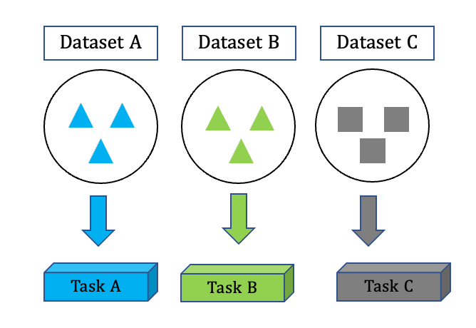
(a) Traditional Machine Learning

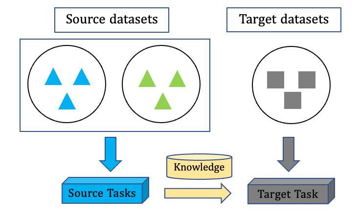
(b) Transfer Learning

Figure 1: Different learning processes between classical machine learning and transfer learning.

1.1 Our Contributions

The main contributions of this paper are the investigations on the transfer learning problem of KRR from the aspects of methodology and theory, which is of fundamental interest to the machine learning community. To some extent, this paper fills the gaps between the practical effectiveness and theoretical guarantees of the kernel-based transfer learning regression. It provides the answer to the question of whether the transfer estimation of KRR can achieve minimax optimality and what types of conditions are required. To our limited knowledge, our work is one of the pioneering works to study the transfer learning problem of KRR with solid theoretical guarantees. The specific contributions can be concluded as follows:

• Methodology novelty: We develop a two-step transfer learning algorithm for the case that the transferable source is known, which solely uses KRR and consists of a debiasing step to enhance the transfer learning accuracy. For those more challenging scenarios where the transferable sources are unknown, we develop a novel sparse aggregation-based transfer learning algorithm of KRR, which aggregates multiple estimators and has the ability to automatically eliminate the effects of negative sources.

• Theoretical assessments: By using the analytic tools for integral operator (Smale & Zhou, 2007; Caponnetto & De Vito, 2007), we establish the upper bound in Theorem 1 for the known transferable source case, and it reveals that with properly chosen regularization parameters, the obtained convergence rate is much sharper than that of the standard KRR estimator where only the target data are used. More importantly, an algorithm-free minimax lower bound is also provided in Theorem 2, which demonstrates that the convergence rate achieved by the proposed estimator implemented in Algorithm 1 is minimax optimal. For a much more challenging case where the transferable source is unknown, we leverage the technical tools and results in Koltchinskii & Yuan (2010) to establish the upper bound in Theorem 4, which indicates that the proposed estimator as described in Algorithm 2 can achieve a comparable rate to that established in Theorem 1 under the known transferable source case.

• Numerical verification: Another contribution of this work is the comprehensive studies on the validity and effectiveness of the proposed algorithms in various synthetic and real-life examples, which further supports the theoretical findings in Theorems 1 and 4, and also provides a better understanding of the proposed two methods.

1.2 Related Works

In the machine learning community, transfer learning has attracted tremendous interest from both practitioners and researchers, and various transfer learning algorithms have been proposed under different settings. Interested readers are referred to Pan & Yang (2010); Weiss et al. (2016) and the references therein for details. Yet, many existing transfer learning methods are proposed under some specific model assumptions, and the theoretical understanding of those methods are still insufficient and have become increasingly popular.

A majority of the existing methods are developed under the linear model assumption. Specifically, Bastani (2021) studies the transfer learning problem of high-dimensional linear regression and proposes a novel two-step estimator, which efficiently combines the source and target data and provides the upper bound of the estimation error. Yet, it only focuses on the case with one source task and assumes that the sample size of the source data is larger than the dimension of the coefficient. Inspired by this pioneering work, Li et al. (2022) consider the problem of multi-source transfer learning in high-dimensional sparse linear regression, and uses the $\ell_{q}$-distance, $0\leq q\leq 1$, as the similarity measure. They also establish the minimax optimal rates under certain technical conditions. Moreover, Tian & Feng (2022) and Li et al. (2023) further consider the estimation and inference problem for the high-dimensional generalized linear model with knowledge transfer, and minimax rate of convergence and asymptotic normality for the debiased estimator are established. To model the data heterogeneity, Zhang & Zhu (2025) focuses on the high-dimensional quantile regression problem under the transfer learning framework. Two convolution smoothing transfer learning algorithms are provided and analogous theoretical guarantees are also established. Note that all the aforementioned methods focus on the linear model case, which is restrictive and difficult to verify in practice.

Recently, transfer learning under the nonparametric setting has also received significant attention. Specifically, Blitzer et al. (2007) and Mansour et al. (2009) consider the nonparametric transfer learning in the context of the general classification problem and provide the uniform convergence bound for the estimator that minimizes a convex combination of source and target empirical risk. In the posterior drift setting, Cai & Wei (2021) proposes a data-driven adaptive classifier for transfer learning of nonparametric classification and conducts the non-asymptotic minimax analysis, which offers valuable statistical insights and motivates many follow-up works. Inspired by this work, Cai & Pu (2023) investigates the transfer learning problem of nonparametric regression, where the $\ell_{1}$-distance is adopted as the similarity measure. Then, a novel confidence thresholding estimator is developed which can achieve the minimax optimality. Yet, it is interesting to point out that they focus on the function class of polynomial functions with Hölder continuity, which is still somewhat restrictive and may suffer computational burden especially when the number of covariates is relatively large. Compared to the local polynomial regression, KRR can better handle data with many covariates and is computationally efficient since it has an explicit solution.

1.3 Paper Organization

The rest of this paper is organized as follows. In Section 2, we introduce some necessary notations and basic knowledge of the kernel-based method and transfer learning under the kernel-based setting. Section 3 formally formulates the transfer learning problem of KRR and two efficient algorithms are developed to handle the cases where the prior information of transferable sources is known and unknown, respectively. Section 4 is devoted to establishing the theoretical guarantees on the proposed algorithms, including the minimax optimal rates. Numerical experiments on synthetic examples and two real applications are provided in Sections 5 and 6. Section 7 contains a brief conclusion and future directions and all the technique details are deferred to the Appendix.

2 Preliminaries

In this section, we introduce some necessary notations, provide some basic background on reproducing kernel Hilbert spaces, and formulate the problem of transfer learning for the kernel-based nonparametric regression.

2.1 Notation

Let $\rho_{\mathop{\bf x}}$ be the probability measure on a compact support $\mathcal{X}\subset\mathbb{R}^{d}$. We use ${\cal L}_{2}(\mathcal{X},\rho_{\mathop{\bf x}})=\{f:\int_{{\mathcal{X}}}f^{2}(\mathop{\bf x})d\rho_{\mathop{\bf x}}<\infty\}$ to denote the space of square-integrable functions with respect to $\rho_{\mathop{\bf x}}$, equipped with the inner product $\langle f,g\rangle_{\rho_{\mathop{\bf x}}}=\int_{\mathcal{X}}f(\mathop{\bf x})g(\mathop{\bf x})d\rho_{\mathop{\bf x}}$ and squared norm $\|f\|^{2}_{\rho_{\mathop{\bf x}}}=\int_{\mathcal{X}}f^{2}(\mathop{\bf x})d\rho_{\mathop{\bf x}}$. In a slightly abuse of notation, we write $\langle\cdot,\cdot\rangle=\langle\cdot,\cdot\rangle_{\rho_{\mathop{\bf x}}}$ for notation simplicity. We use $\operatorname{Tr}(\cdot)$ to denote the trace of an operator or a matrix, and $|{\cal A}|$ to denote the cardinality of a set $\cal A$. For two sequences $\{a_{k}\}_{k\geq 1}$ and $\{b_{k}\}_{k\geq 1}$, we write $a_{k}\lesssim b_{k}$ if $a_{k}\leq cb_{k}$ for some universal constant $c>0$, and $a_{k}\gtrsim b_{k}$ if $a_{k}\geq cb_{k}$. And we say $a_{k}\asymp b_{k}$ if both $a_{k}\lesssim b_{k}$ and $a_{k}\gtrsim b_{k}$ hold. For two random variable sequences $\{A_{k}\}_{k\geq 1}$ and $\{B_{k}\}_{k\geq 1}$, we denote $A_{k}=O_{P}(B_{k})$ if for any $\epsilon>0$, there exists a finite constant $M_{\varepsilon}>0$ such that $\sup_{k}P(|A_{k}/B_{k}|>M_{\varepsilon})<\epsilon$ and denote $A_{k}=o_{P}(B_{k})$ if $A_{k}/B_{k}\rightarrow 0$ in probability. We use $I$ to represent the identity operator throughout this paper.

2.2 Reproducing Kernel

KRR is one of the most powerful tools in machine learning, where the true target function is often believed to belong to a reproducing kernel Hilbert space (RKHS), and has become a time-proven popular mainstay in the literature of machine learning (Murphy, 2012).

Let ${\cal H}_{K}$ denote the RKHS induced by a symmetric, positive and semi-definite kernel function $K:{\cal X}\times{\cal X}\rightarrow\mathbb{R}$ and we define its equipped norm as $\|\cdot\|^{2}_{K}={\langle\cdot,\cdot\rangle_{K}}$ with the endowed inner product $\langle\cdot,\cdot\rangle_{K}$. We also define $K_{\mathop{\bf x}}:=K(\mathop{\bf x},\cdot)\in{\cal H}_{K}$, for each $\mathop{\bf x}\in\mathcal{X}$ and assume that $\sup_{\mathop{\bf x}\in{\cal X}}\sqrt{K(\mathop{\bf x},\mathop{\bf x})}\leq\kappa$ for some positive constant $\kappa$. An important property in ${\cal H}_{K}$ is called the reproducing property, stating that

$$\langle f,K_{\mathop{\bf x}}\rangle_{K}=f(\mathop{\bf x}),\quad\text{for any}\ \ f\in{\cal H}_{K}.$$

Note that the kernel complexity of ${\cal H}_{K}$ (Mendelson & Neeman, 2010; Koltchinskii & Yuan, 2010) is fully characterized by an integral operator $L_{K}:{\cal L}_{2}(\mathcal{X},\rho_{\mathop{\bf x}})\rightarrow{\cal H}_{K}$ , which is defined as

$$L_{K}f=\int K_{\mathop{\bf x}}f(\mathop{\bf x})d\rho_{\mathop{\bf x}}.$$

It is well-known that the integral operator $L_{K}$ is positive, trace-class, self-adjoint, and thus a compact operator. The spectral theorem implies that $L_{K}f=\sum_{k=1}^{\infty}\mu_{k}\langle f,\psi_{k}\rangle\psi_{k}$, where $\mu_{1}\geq\mu_{2}\geq\cdots\geq 0$ is a sequence of nonnegative eigenvalues and $\{\psi_{k}\}_{k=1}^{\infty}$ are the corresponding orthonormal basis in ${\cal L}_{2}\big{(}{\cal X},\rho_{\mathop{\bf x}}\big{)}$.

2.3 Multi-source, Target Model and Similarity Measure

We now formulate the transfer learning problem for KRR. Suppose that we collect $m+1$ datasets: the target dataset ${\cal T}=\{({\mathop{\bf x}}^{(0)}_{i},y^{(0)}_{i})\}_{i=1}^{n_{0}}$ and multi-source datasets ${\cal S}^{(k)}=\{({\mathop{\bf x}}^{(k)}_{i},y^{(k)}_{i})\}_{i=1}^{n_{k}}$ for $k=1,\ldots,m$, which are generated by the following mechanism that

$$\{({\mathop{\bf x}}^{(k)}_{i},y^{(k)}_{i})\}_{i=1}^{n_{k}}\overset{i.i.d.}{\sim}\rho^{(k)}_{\mathop{\bf x},y},\ k=0,1,\ldots,m,$$

for some unknown joint distributions $\rho^{(k)}_{\mathop{\bf x},y}$ supported on $\mathcal{X}\times\mathbb{R}$. In this paper, we consider the scenario where the sample size of the target data is much smaller than that of multi-source data due to the difficulties in data collection or high costs. The conditional distribution on $\mathbb{R}$ given $\mathop{\bf x}$ is denoted by $\rho^{(k)}_{y|\mathop{\bf x}}$. Moreover, we assume that $\rho^{(k)}_{\mathop{\bf x},y}=\rho^{(k)}_{y|\mathop{\bf x}}\rho_{\mathop{\bf x}},\leavevmode\nobreak\ k=0,\ldots,m$, and then it requires the conditional distributions between the source and target data may be different, while the marginal distributions are the same. Similar requirements are also assumed in the literature of transfer learning (Cai & Wei, 2021; Cai & Pu, 2023). Consider a general regression setting that

$$y_{i}^{(k)}=f_{\rho}^{(k)}({\mathop{\bf x}}^{(k)}_{i})+\epsilon_{i}^{(k)},$$

where $\epsilon_{i}^{(k)}$ is a random noise with $E[\epsilon_{i}^{(k)}|{\mathop{\bf x}}^{(k)}_{i}]=0$ for $i=1,\ldots,n_{k}$ and $k=0,1,\ldots,m$. Thus, there holds $f_{\rho}^{(k)}({\mathop{\bf x}}^{(k)})=\int y^{(k)}d\rho^{(k)}_{y|{\mathop{\bf x}}^{(k)}}$, and we further assume that $f_{\rho}^{(k)}\in{\cal H}_{K}$ in this paper.

Our primary interest is to achieve a much more accurate estimation and prediction performance for the KRR by utilizing the target data $\mathcal{T}$ and the useful information provided by the multi-source data $\mathcal{S}^{(k)}$, $k=1,\ldots,m$. Ideally, if the source function $f_{\rho}^{(k)}$ is close to the target function $f_{\rho}^{(0)}$, we can improve the accuracy of estimating $f_{\rho}^{(0)}$ in the target domain by incorporating information from $\mathcal{S}^{(k)}$ in the auxiliary source domains. Clearly, the effectiveness of such a transfer learning strategy heavily relies on quantifying the similarity between $f_{\rho}^{(0)}$ and $f_{\rho}^{(k)}$. Therefore, we define the $k$-th contrast function as $\delta^{(k)}=f_{\rho}^{(0)}-f_{\rho}^{(k)}$ to measure the similarity between the target and source function. Specifically, for some small $h>0$, we say the $k$-th source function $f_{\rho}^{(k)}$ is $h$-transferable if

$$\|\delta^{(k)}\|_{K}=\|f_{\rho}^{(0)}-f_{\rho}^{(k)}\|_{K}\leq h,$$

and then, the $h$-transferable source index set can be defined as

$${\cal A}_{h}=\big{\{}k:\|\delta^{(k)}\|_{K}\leq h,1\leq k\leq m\big{\}}.$$

It is worthy pointing out that the transfer efficiency depends on the choice of similarity level $h$ in that a smaller $h$ may result in a better estimation accuracy by leveraging information from similar transferable source data. Yet, when $h$ shrinks to a near-zero level, it may lead to the case that ${\cal A}_{h}=\emptyset$ and then all the source data are useless.

3 Transfer Learning for KRR

In this section, we propose two efficient transfer learning methods for KRR to deal with those cases where ${\cal A}_{h}$ is known and unknown, respectively. For notation simplicity, we denote $n_{{\cal A}_{h}}=\sum_{k\in{\cal A}_{h}}n_{k}$, $\eta_{k}=\frac{n_{k}}{n_{{\cal A}_{h}}+n_{0}}$ for $k\in\{0\}\cup{\cal A}_{h}$, and $m_{h}=|{\cal A}_{h}|+1$. We also denote $f^{p}_{\rho}=\sum_{k\in\{0\}\cup{\cal A}_{h}}\eta_{k}f^{(k)}_{\rho}$.

3.1 Two-step Transfer Learning with Known Transferable Sources

Inspired by the ideas in Bastani (2021) and Li et al. (2022), when ${\cal A}_{h}$ is known given some pre-specified $h$, a two-step transfer learning algorithm named ${\cal A}_{h}$-TKRR is proposed to leverage the information in ${\cal S}_{{\cal A}_{h}}=\{{\cal S}^{(k)}:k\in{\cal A}_{h}\}$. The main strategy is to firstly transfer the information from the source data by pooling ${\cal S}_{{\cal A}_{h}}$ and ${\cal T}$ together for obtaining a rough estimator of $f^{(0)}_{\rho}$ that

$$\widehat{f}^{p}=\mathop{\rm argmin}_{f\in{\cal H}_{K}}\Big{\{}\frac{1}{n_{{\cal A}_{h}}+n_{0}}\sum_{k\in\{0\}\cup{\cal A}_{h}}\sum_{i=1}^{n_{k}}\big{(}f({\mathop{\bf x}}^{(k)}_{i})-y_{i}^{(k)}\big{)}^{2}+\lambda_{1}\|f\|_{K}^{2}\Big{\}},$$ (1)

where $\lambda_{1}$ denotes the regularization parameter. By the representer theorem (Kimeldorf & Wahba, 1971), the minimizer of the optimization task (1) must have a finite form that

$$\widehat{f}^{p}(\mathop{\bf x})=\sum_{k\in\{0\}\cup{\cal A}_{h}}\sum_{i=1}^{n_{k}}\widehat{\beta}_{i}^{(k)}K(\mathop{\bf x},{\mathop{\bf x}}_{i}^{(k)}),$$

where $\{\widehat{\beta}_{i}^{(k)}\}^{\prime}s$ are the estimated representer coefficients. To better understand the transferring step, we define $f_{\lambda_{1}}^{p}$ as the minimizer of the expected version of (1) that

$$f_{\lambda_{1}}^{p}=\mathop{\rm argmin}_{f\in{\cal H}_{K}}\Big{\{}\sum_{k\in\{0\}\cup{\cal A}_{h}}\frac{n_{k}}{n_{{\cal A}_{h}}+n_{0}}E\big{[}f({\mathop{\bf x}}^{(k)}_{i})-y_{i}^{(k)}\big{]}^{2}+\lambda_{1}\|f\|_{K}^{2}\Big{\}},$$

and thus it satisfies $\sum_{k\in\{0\}\cup{\cal A}_{h}}\eta_{k}\int\big{(}f_{\lambda_{1}}^{p}(\mathop{\bf x})-f_{\rho}^{(k)}(\mathop{\bf x})\big{)}K_{\mathop{\bf x}}d\rho_{\mathop{\bf x}}+\lambda_{1}f_{\lambda_{1}}^{p}=0$ by the optimality condition of $f_{\lambda_{1}}^{p}$. Clearly, simple algebra yields $f_{\lambda_{1}}^{p}=f_{\rho}^{(0)}-\Delta_{\rho}$, where $\Delta_{\rho}=(L_{K}+\lambda_{1}I)^{-1}\big{(}\lambda_{1}f_{\rho}^{(0)}+L_{K}(f_{\rho}^{(0)}-f_{\rho}^{p})\big{)}$ which denotes the expected version of the bias in the transferring step.

Algorithm 1 : ${\cal A}_{h}$-TKRR

0:  multi-source data $\mathcal{S}^{(k)}=\{({\mathop{\bf x}}^{(k)}_{i},y^{(k)}_{i})\}_{i=1}^{n_{k}}$, $k=1,\ldots,m$, target data $\mathcal{T}=\{({\mathop{\bf x}}^{(0)}_{i},y^{(0)}_{i})\}_{i=1}^{n_{0}}$, index set ${\cal A}_{h}$, the pre-specified parameters $\lambda_{1}$ and $\lambda_{2}$.

1:  Transferring step. Compute $\widehat{f}^{p}$ by solving (1);

2:  Debiasing step. Compute $\widehat{w}^{(0)}_{i}=y_{i}^{(0)}-\widehat{f}^{p}({\mathop{\bf x}}_{i}^{(0)})$, $i=1,\ldots,n_{0}$ and obtain $\widehat{f}^{\text{de}}$ by solving (2);

3:  Let $\widehat{f}=\widehat{f}^{p}+\widehat{f}^{\text{de}}$.

3:  The final estimator $\widehat{f}$.

Note that the first term of $\Delta_{\rho}$ is known as the approximation error in literature (Smale & Zhou, 2007), and it is necessary to debias the second term of $\Delta_{\rho}$ which comes from the transferring procedure. Precisely, the debiasing step is motivated by the fact that $(L_{K}+\lambda_{1}I)^{-1}\big{(}L_{K}(f_{\rho}^{(0)}-f_{\rho}^{p})\big{)}$ is the solution of

$$\mathop{\rm argmin}_{f\in{\cal H}_{K}}\Big{\{}E\big{[}f({\mathop{\bf x}}^{(0)}_{i})-\big{(}y_{i}^{(0)}-f_{\rho}^{p}({\mathop{\bf x}}_{i}^{(0)})\big{)}\big{]}^{2}+\lambda_{1}\|f\|_{K}^{2}\Big{\}}.$$

It is thus natural to approximate the transferring bias by fitting KRR on the dataset $\{({\mathop{\bf x}}^{(0)}_{i},y_{i}^{(0)}-f_{\rho}^{p}({\mathop{\bf x}}_{i}^{(0)})\}$. With $f_{\rho}^{p}({\mathop{\bf x}}_{i}^{(0)})$ replaced by its estimate $\widehat{f}^{p}({\mathop{\bf x}}_{i}^{(0)})$, we compute the residuals $\widehat{w}^{(0)}_{i}=y_{i}^{(0)}-\widehat{f}^{p}({\mathop{\bf x}}_{i}^{(0)})$, $i=1,\ldots,n_{0}$, and then obtain a debiased estimator by solving the following optimization task

$$\widehat{f}^{\text{de}}=\mathop{\rm argmin}_{f\in{\cal H}_{K}}\Big{\{}\frac{1}{n_{0}}\sum_{i=1}^{n_{0}}\big{(}f({\mathop{\bf x}}^{(0)}_{i})-\widehat{w}_{i}^{(0)}\big{)}^{2}+\lambda_{2}\|f\|_{K}^{2}\Big{\}},$$ (2)

where $\lambda_{2}$ denotes the regularization parameter. Again, by the representer theorem, we have

$$\widehat{f}^{\text{de}}(\mathop{\bf x})=\sum_{i=1}^{n_{0}}\widetilde{\beta}_{i}^{(0)}K(\mathop{\bf x},{\mathop{\bf x}}_{i}^{(0)}).$$

Combining the above two estimators, we derive the final estimator of $f^{(0)}_{\rho}$ that

$$\widehat{f}(\mathop{\bf x})=\widehat{f}^{p}(\mathop{\bf x})+\widehat{f}^{\text{de}}(\mathop{\bf x})=\sum_{i=1}^{n_{0}}(\widetilde{\beta}_{i}^{(0)}+\widehat{\beta}_{i}^{(0)})K(\mathop{\bf x},{\mathop{\bf x}}_{i}^{(0)})+\sum_{k\in{\cal A}_{h}}\sum_{i=1}^{n_{k}}\widehat{\beta}_{i}^{(k)}K(\mathop{\bf x},{\mathop{\bf x}}_{i}^{(k)}).$$ (3)

The proposed two-step transfer learning algorithm is summarized in Algorithm 1.

A theoretical example is considered to provide some insightful understanding of Algorithm 1, where we assume that ${\cal A}_{h}=\{1,2,3\}$ is known and the illustration is depicted in Figure 2. Specifically, the standard KRR estimator $\widehat{f}_{KRR}$ is obtained only using the target data, and it is well-known that its optimal convergence rate is $r_{1}=O_{P}(n_{0}^{-\frac{r}{2r+\alpha}})$ (Caponnetto & De Vito, 2007). Note that $r_{1}$ is treated as the radius of the gray circle centering at $f_{\rho}^{(0)}$ in Figure 2. In the transferring step, the estimator $\widehat{f}^{p}$ marked in orange is obtained by pooling all the source data indexed by ${\cal A}_{h}$ and target data. After the debiasing step, the final estimator $\widehat{f}$ is obtained and is marked as the green point in Figure 2. As shown in Theorem 1 of Section 4, the convergence rate of $\widehat{f}$ is $r_{2}=O_{P}\big{(}(n_{{\cal A}_{h}}+n_{0})^{-\frac{r}{2r+\alpha}}+h^{\frac{\alpha}{1+\alpha}}n_{0}^{-\frac{1}{2+2\alpha}}\big{)}$, which is much smaller than $r_{1}$ under mild conditions. This further supports the advantage of the proposed method implemented in Algorithm 1.

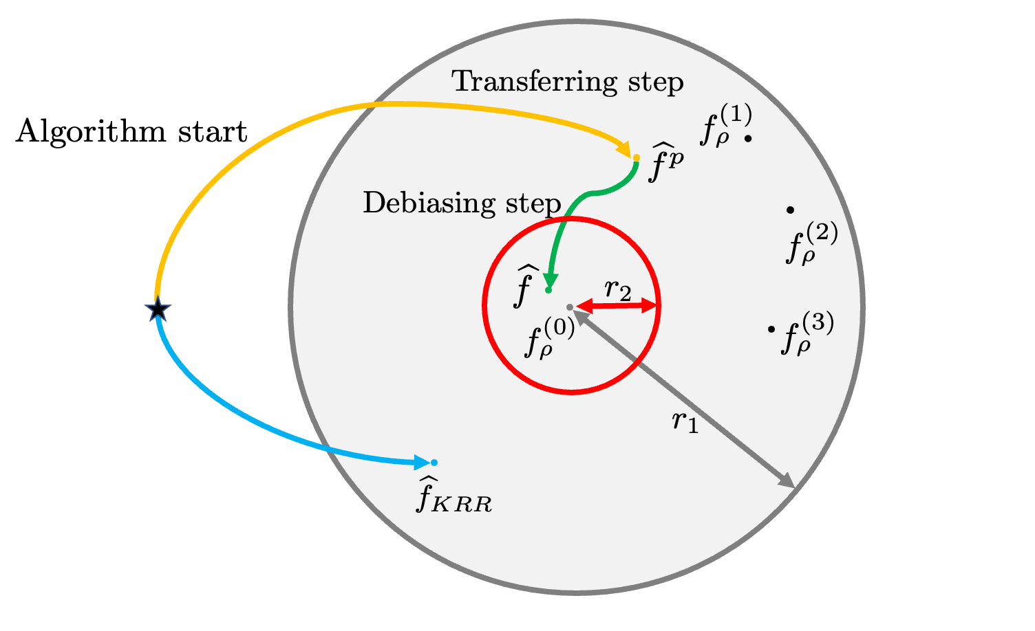
Figure 2: Illustration of how Algorithm 1 leads to a better estimator of $f_{\rho}^{(0)}$ in an theoretical example where ${\cal A}_{h}=\{1,2,3\}$, and $f_{\rho}^{(0)}$,$f_{\rho}^{(1)}$,$f_{\rho}^{(2)}$,$f_{\rho}^{(3)}$ are the corresponding target and source functions.

3.2 Transfer Learning with Unknown Transferable Sources

The success of Algorithm 1 requires the prior knowledge of ${\cal A}_{h}$. In practice, it is unrealistic to know ${\cal A}_{h}$ in advance, and brute-force transfer can be detrimental to the prediction performance when the source and target data are not closely related (Pan & Yang, 2010; Weiss et al., 2016). To tackle these problems, we propose a sparse aggregation-based transfer learning KRR algorithm named SA-TKRR, which is robust to the negative sources. In sharp contrast to ${\cal A}_{h}$-TKRR which highly depends on the choice of the pre-specified $h$, SA-TKRR is able to automatically search the optimal choice of $h$ in an efficient way with a theoretical guarantee.

Now we introduce SA-TKRR in detail. Specifically, we first randomly and uniformly divide the target data $\mathcal{T}$ into two subsets, $\mathcal{T}_{1}$ and ${\cal T}_{2}$. For notation simplicity, we denote ${\cal S}^{(0)}={\cal T}_{1}$. Then, we fit the standard KRR on each $\mathcal{S}^{(k)}$ to obtain the estimators $\widehat{f}^{(k)}$ that

$$\widehat{f}^{(k)}=\mathop{\rm argmin}_{f\in{\cal H}_{K}}\Big{\{}\frac{1}{n_{k}}\sum_{i=1}^{n_{k}}\big{(}f({\mathop{\bf x}}^{(k)}_{i})-y_{i}^{(k)}\big{)}^{2}+\lambda^{(k)}\|f\|_{K}^{2}\Big{\}},$$ (4)

for $k=0,1,\ldots,m$. Next, we compute the estimated contrast function

$$\widehat{\delta}^{(k)}=\widehat{f}^{(k)}-\widehat{f}^{(0)}.$$ (5)

Note that the RKHS-norm $\|\widehat{\delta}^{(k)}\|_{K}=\|\widehat{f}^{(k)}-\widehat{f}^{(0)}\|_{K}$ can be directly computed by using the the representer theorem (Kimeldorf & Wahba, 1971) and the property of inner product $\langle\cdot,\cdot\rangle_{K}$. Thus, we can calculate the estimated rank $\widehat{R}_{k}$ of $\|\widehat{\delta}^{(k)}\|_{K}$ in $\{\|\widehat{\delta}^{(1)}\|_{K},\ldots,\|\widehat{\delta}^{(m)}\|_{K}\}$. It is clear that the smaller $\|\widehat{\delta}^{(k)}\|_{K}$ is, the closer the $k$-th source function and the target function are. Once the ranks $\{\widehat{R}_{k}\}_{k=1}^{m}$ are obtained, we define an index set that

$$\widehat{{\cal A}}_{\ell}=\{k:\widehat{R}_{k}\leq\ell,k=1,\ldots,m\},$$ (6)

for $\ell=1,\ldots,m$, and then fit ${\cal A}_{h}$-TKRR in Algorithm 1 with the target data $\mathcal{T}_{1}$, source data $\{\mathcal{S}^{(k)}\}_{k\in\widehat{{\cal A}}_{\ell}}$ and parameters $\lambda_{1}^{(\ell)},\lambda_{2}^{(\ell)}$ to obtain an intermediate estimator $\widehat{f}_{\ell}$. Note that we define $\widehat{{\cal A}}_{0}=\emptyset$ and thus $\widehat{f}_{0}=\widehat{f}^{(0)}$.

Algorithm 2 SA-TKRR

0:  ${\cal T}=\{({\mathop{\bf x}}_{i}^{(0)},y_{i}^{(0)})\}_{i=1}^{n_{0}}$, ${\cal S}^{(k)}=\{({\mathop{\bf x}}_{i}^{(k)},y_{i}^{(k)})\}_{i=1}^{n_{k}}$, the pre-specified parameters $\{\lambda^{(k)}\}_{k\geq 0},\{\lambda_{1}^{(\ell)}\}_{\ell\geq 1},\{\lambda_{2}^{(\ell)}\}_{\ell\geq 1}$, $c$ and $\phi$,

1:  Randomly and uniformly split $\mathcal{T}$ into $\mathcal{T}_{1}$ and $\mathcal{T}_{2}$.

2:  Fit (4) on each ${\cal S}^{(k)}$ with regularization parameter $\lambda^{(k)}$ for $k=0,1,\ldots,m$ to obtain $\widehat{f}^{(k)}$ where ${\cal S}^{(0)}={\cal T}_{1}$.

3:  For $k=1,\ldots,m$, compute the estimated contrast function $\widehat{\delta}^{(k)}$ based on (5).

4:  For $k=1,\ldots,m$, compute the rank $\widehat{R}_{k}$ of $\|\widehat{\delta}^{(k)}\|_{K}$ in $\{\|\widehat{\delta}^{(k)}\|_{K}\}_{k=1}^{m}$.

5:  For $\ell=1,\ldots,m$, let $\widehat{{\cal A}}_{\ell}=\{k:\widehat{R}_{k}\leq\ell,1\leq k\leq m\}$ and obtain $\widehat{f}_{\ell}$ by Algorithm 1 with $\mathcal{T}_{1}$ and $\{\mathcal{S}^{(k)}\}_{k\in\widehat{{\cal A}}_{\ell}}$, regularization parameters $\lambda_{1}^{(\ell)}$ and $\lambda_{2}^{(\ell)}$. Moreover, let $\widehat{f}_{0}=\widehat{f}^{(0)}$.

6:  Run the hyper-sparse aggregate algorithm with $\mathcal{F}=\{\widehat{f}_{0},\ldots,\widehat{f}_{m}\}$, $\mathcal{T}_{2}$ and parameters $c,\phi$ to obtain $\widehat{f}_{a}$ based on (7).

6:  $\widehat{f}_{a}$.

Then, we obtain a candidate function set ${\cal F}=\{\widehat{f}_{0},\widehat{f}_{1},\ldots,\widehat{f}_{m}\}$, and further use an optimal aggregation procedure named the hyper-sparse aggregation algorithm (Gaîffas & Lecué, 2011) to construct a convex combination $\widetilde{f}$ of the functions in $\cal F$ such that the risk for $\widetilde{f}$ is as close as possible to the minimum risk over $\cal F$. To be more precise, we first randomly and uniformly split ${\cal T}_{2}$ into two subsets ${\cal T}_{21}$ and ${\cal T}_{22}$. Then, given some pre-specified parameters $\phi$ and $c$, we define a random subset of $\mathcal{F}$ as

$$\widehat{\cal F}_{1}=\Big{\{}f\in{\cal F}:\ \widehat{\cal E}_{{\cal T}_{21}}(f)\leq\widehat{\cal E}_{{\cal T}_{21}}(\widehat{f}_{{\cal T}_{21}})+c\max\big{(}\phi\|\widehat{f}_{{\cal T}_{21}}-f\|_{n,1},\phi^{2}\big{)}\Big{\}},$$

where $\widehat{\cal E}_{{\cal T}_{21}}(f)=\frac{1}{|{\cal T}_{21}|}\sum_{(\mathop{\bf x}_{i},y_{i})\in{\cal T}_{21}}(y_{i}-f({\mathop{\bf x}}_{i}))^{2}$, $\widehat{f}_{{\cal T}_{21}}=\mathop{\rm argmin}_{f\in\mathcal{F}}\widehat{\cal E}_{{\cal T}_{21}}(f)$ and $\|f\|_{n,1}^{2}=\frac{1}{|{\cal T}_{21}|}\sum_{(\mathop{\bf x}_{i},y_{i})\in{\cal T}_{21}}f^{2}({\mathop{\bf x}}_{i})$. Moreover, we define

$$\widehat{\cal F}_{2}=\big{\{}tf_{1}+(1-t)f_{2}:\ f_{1},\ f_{2}\in\widehat{\mathcal{F}}_{1}\ \text{and}\ 0\leq t\leq 1\big{\}},$$

which is the collection of convex combinations of at most two functions in $\mathcal{F}$. Then, the SA-TKRR estimator $\widehat{f}_{a}$ can be obtained as

$$\widehat{f}_{a}=\mathop{\rm argmin}_{f\in\widehat{\cal F}_{2}}\widehat{\cal E}_{{\cal T}_{22}}(f).$$ (7)

It is shown in Gaîffas & Lecué (2011) that (7) has the explicit solution with the form that $\widehat{f}_{a}=\tilde{t}\widehat{f}_{\ell_{1}}+(1-\tilde{t})\widehat{f}_{\ell_{2}}$ where $\ell_{1},\ell_{2}\in\{0,\ldots,m\}$ and $\ell_{1}\neq\ell_{2}$ and the weight $\tilde{t}$ can be directly calculated.

Note that if $\tilde{t}=1$ and ${\ell}_{1}=0$, $\widehat{f}_{a}$ reduces to the standard KRR estimator, which only uses the target data. This ensures that the SA-TKRR estimator can deal with the case that all the source data are negative, and then only the target data are used. The proposed SA-TKRR algorithm is summarized in Algorithm 2. It is also interesting to notice that the implementation of Algorithm 2 does not require the explicit specification of $h$, and can automatically select the best choice of $h$. In fact, as shown in Theorem 4 of Section 4, Algorithm 2 can automatically select the best threshold $h$ leading to the minimum of the theoretical upper bound. In sharp contrast to most existing algorithms dealing with unknown transferable sources (Li et al., 2022; Tian & Feng, 2022; Jun et al., 2022), the proposed algorithm is much more robust, general and computationally efficient. Its superior performance is also validated by a variety of numerical examples in Sections 5.2 and 6.2. It is also interesting to point out that at the end of Algorithm 2, the estimators $\widehat{f}_{\ell_{1}}$ and $\widehat{f}_{\ell_{2}}$ can be retrained by using the entire target data $\mathcal{T}$ and the corresponding source data $\{\mathcal{S}^{(k)}\}_{k\in\widehat{{\cal A}}_{\ell_{1}}}$ and $\{\mathcal{S}^{(k)}\}_{k\in\widehat{{\cal A}}_{\ell_{2}}}$, respectively, to sufficiently utilize the target data.

4 Theoretical Guarantee

In this section, we first provide the theoretical guarantee for ${\cal A}_{h}$-TKRR where ${\cal A}_{h}$ is known in Section 4.1. Particularly, a theoretical upper bound of ${\cal A}_{h}$-TKRR estimator is established in Theorem 1, which is also verified as minimax optimal in Theorem 2. We also summarize the detailed convergence rates for some special kernel classes. In Section 4.2, we provide the theoretical results for SA-TKRR without the known set ${\cal A}_{h}$, including the consistency of $\widehat{{\cal A}}_{\ell}$ in Theorem 3 and the theoretical upper bound of the SA-TKRR estimator $\widehat{f}_{a}$ in Theorem 4.

We first define a quantity named effective dimension (Caponnetto & De Vito, 2007) to measure the complexity of ${\cal H}_{K}$ with respect to $\rho_{\mathop{\bf x}}$ that

$${\cal N}(\lambda)=\operatorname{Tr}\big{(}(L_{K}+\lambda I)^{-1}L_{K}\big{)},\ \ \text{for any}\ \lambda>0,$$

which in fact is the trace of the operator $(L_{K}+\lambda I)^{-1}L_{K}$. The following technical assumptions are required to establish the theoretical results.

Assumption 1.

Suppose that for each $k=0,1,\ldots,m$, $E[(y^{(k)})^{2}]<\infty$ and

$$\int\big{(}e^{\frac{|y^{(k)}-f^{(k)}_{\rho}({\mathop{\bf x}}^{(k)})|}{B}}-\frac{|y^{(k)}-f_{\rho}^{(k)}({\mathop{\bf x}}^{(k)})|}{B}-1\big{)}d\rho^{(k)}_{y|{\mathop{\bf x}}^{(k)}}\leq\frac{\gamma^{2}}{2B^{2}},\quad\text{for any}\ \ {\mathop{\bf x}}\in\mathcal{X},$$

where $B$ and $\gamma$ are some positive constants.

Assumption 2.

There exist some constants $\alpha\in(0,1]$ and $Q\geq 1$ such that ${\cal N}(\lambda)\leq Q\lambda^{-\alpha},$ where $Q$ is independent of $\lambda$.

Assumption 3.

There exists some constant $\frac{1}{2}\leq r\leq 1$ such that for each $k=0,1,\ldots,m$, there holds

$$f_{\rho}^{(k)}=L_{K}^{r}g_{\rho}^{(k)},\ \text{for some}\ g_{\rho}^{(k)}\in{\cal L}_{2}({\cal X},\rho_{\mathop{\bf x}})$$

where $L_{K}^{r}$ denotes the $r$-th power of $L_{K}$.

Assumption 1 characterizes the distributions of the noise terms in the source and target models, which is satisfied when the noise term is uniformly bounded, Guassian or sub-Guassian distributed. It is a common assumption and is widely used in the literature of machine learning (Caponnetto & De Vito, 2007). It is interesting to point out that Assumption 1 also implies that $\int(y^{(k)}-f_{\rho}^{(k)}({\mathop{\bf x}}^{(k)}))^{b}d\rho^{(k)}_{y|{\mathop{\bf x}}^{(k)}}\leq\frac{1}{2}b!\gamma^{2}B^{b-2}$ for all $b\geq 2$. Assumption 2 controls the complexity of the considered ${\cal H}_{K}$. As pointed out by Lin et al. (2020), when $\alpha=1$, it always holds by taking $Q=\operatorname{Tr}(L_{K})\leq\kappa^{2}$ and when $0<\alpha<1$, it is more general than the eigenvalue decaying assumption in literature (Caponnetto & De Vito, 2007; He et al., 2021). Assumption 3 is a regularity condition on the source and target regression functions, and is also commonly assumed in literature (Smale & Zhou, 2007; Caponnetto & De Vito, 2007; Guo et al., 2017). Note that $r$ controls the smoothness of the regression function $f_{\rho}^{(k)}$, where a larger $r$ indicates a smoother function.

4.1 Optimal Convergence Rates for ${\cal A}_{h}$-TKRR

The following theorem establishes the upper bound of the ${\cal A}_{h}$-TKRR estimator.

Theorem 1 (Upper bound of ${\cal A}_{h}$-TKRR).

Suppose that Assumptions 1- 3 are satisfied. With the choices of $\lambda_{1}\asymp(n_{{\cal A}_{h}}+n_{0})^{-\frac{1}{2r+\alpha}}$ and $\lambda_{2}\asymp h^{-\frac{2}{1+\alpha}}n_{0}^{-\frac{1}{1+\alpha}}$, for any $\delta\in(0,1)$ satisfying

$$C_{0}\exp\Big{\{}-\min\big{\{}(n_{{\cal A}_{h}}+n_{0})^{\frac{2r+\alpha-1}{2(2r+\alpha)}}(\log(n_{{\cal A}_{h}}+n_{0}))^{-\frac{1}{2}},h^{-\frac{2}{1+\alpha}}{{n_{0}^{\frac{\alpha}{2+2\alpha}}}{(\log n_{0})^{-\frac{1}{2}}}}\big{\}}\Big{\}}\leq\delta,$$

it holds with probability at least $1-\delta$ that

$$\|\widehat{f}-f_{\rho}^{(0)}\|_{\rho_{\mathop{\bf x}}}\leq\underbrace{C_{1}(n_{{\cal A}_{h}}+n_{0})^{-\frac{r}{2r+\alpha}}\log\frac{12m_{h}}{\delta}}_{\text{Transferring error}}+\underbrace{C_{2}h^{\frac{\alpha}{1+\alpha}}n_{0}^{-\frac{1}{2\alpha+2}}\log\frac{12}{\delta}}_{\text{Debiasing error}},$$ (8)

where $C_{0},C_{1}$ and $C_{2}$ are some universal constants.

The proof of Theorem 1 is provided in Appendix B. The established upper bound consists of two terms which are related to the target sample size $n_{0}$, source sample size $n_{{\cal A}_{h}}$, and the similarity level $h$. Note that a larger $h$ may lead to a larger size of transferable source data, and thus may further reduce the transferring error at the cost of increasing the debiasing error. Specifically, when $h\lesssim n_{0}^{-\frac{2r-1}{4r+2\alpha}}$ and $n_{{\cal A}_{h}}\gtrsim n_{0}$, the upper bound in (8) is dominated by the transferring error term $(n_{{\cal A}_{h}}+n_{0})^{-\frac{r}{2r+\alpha}}$, which is much sharper than the convergence rate $n_{0}^{-\frac{r}{2r+\alpha}}$ of the standard KRR where only the target data is used (Caponnetto & De Vito, 2007). When $h=0$ and ${\cal A}_{0}=\emptyset$, the debiasing error term in (8) turns to zero and the transferring error terms degenerate to $n_{0}^{-\frac{r}{2r+\alpha}}$, which implies that no informative source data can be used to improve the estimation accuracy. Moreover, the upper bound in (8) becomes sharper with the increasing of the source data size $n_{{\cal A}_{h}}$, and then becomes stable if $(n_{{\cal A}_{h}}+n_{0})^{-\frac{r}{2r+\alpha}}\asymp h^{\frac{\alpha}{1+\alpha}}n_{0}^{-\frac{1}{2+2\alpha}}$ in the sense that the convergence rate can not be further improved by increasing $n_{{\cal A}_{h}}$.

Remark 1.

We summarize those more explicit convergence rates for some special kernel classes, where two types of kernel are considered as follows. (i). $\beta$-polynomial decay: Polynomial decay kernels have eigen-expansion such that $\mu_{j}\lesssim j^{-{\beta}}$, which includes the Sobolev and Laplacian kernels. It can be verified that this condition implies Assumption 2 holds with $\alpha=1/\beta$ (Caponnetto & De Vito, 2007). Hence, as a straightforward consequence, the convergence rate in Theorem 1 turns to $O_{P}\big{(}(n_{{\cal A}_{h}}+n_{0})^{-\frac{r\beta}{2r\beta+1}}+h^{\frac{1}{1+\beta}}n_{0}^{-\frac{\beta}{2\beta+2}}\big{)}$; (ii). $\gamma$-exponential decay: Exponential decay kernels have eigen-expansion such that $\mu_{j}\lesssim\exp(-j^{{\gamma}})$. A well-known example is the Gaussian kernel. Interestingly, Assumption 2 holds with an arbitrarily small $\alpha>0$ for the Gaussian kernel, and also leads to the convergence rate in Theorem 1 holding for arbitrarily small $\alpha>0$.

Now we turn to establish the lower bounds for all learning methods and show that the ${\cal A}_{h}$-TKRR estimator is (nearly) optimal. For notation simplicity, we denote ${\cal Z}^{n_{0}+n_{{\cal A}_{h}}}=\big{\{}{{({\mathop{\bf x}}^{(k)}_{i},y^{(k)}_{i})}_{i=1}^{n_{k}}}\big{\}}_{k\in\{0\}\cup{\cal A}_{h}}$ as the data consisting of the target data and all the transferable source data. Moreover, we consider the set of joint probability distributions on ${\cal Z}^{n_{0}+n_{{\cal A}_{h}}}$ that ${\cal P}_{h}=\big{\{}\otimes_{k\in\{0\}\cup{\cal A}_{h}}{\rho_{\mathop{\bf x},y}^{(k)}}^{\otimes n_{k}}\big{\}}$, where $\otimes_{k=1}^{J}\rho_{\mathop{\bf x},y}^{(k)}=\rho_{\mathop{\bf x},y}^{(1)}\otimes\cdots\otimes\rho_{\mathop{\bf x},y}^{(J)}$ represents the product of probability distributions and ${\rho_{\mathop{\bf x},y}^{(k)}}^{\otimes n_{k}}=\otimes_{i=1}^{n_{k}}{\rho_{\mathop{\bf x},y}^{(k)}}$.

Theorem 2 (Minimax lower bound).

Let $\mathcal{P}_{0}\subset\mathcal{P}_{h}$ consist of all the distributions satisfying Assumptions 1-3. Then, for any estimator $\widehat{f}_{0,h}$ based on the data ${\cal Z}^{n_{0}+n_{{\cal A}_{h}}}$, there exists a joint probability distribution in $\mathcal{P}_{0}$ from which ${\cal Z}^{n_{0}+n_{{\cal A}_{h}}}$ is generated such that

$$P\big{(}\|\widehat{f}_{0,h}-f_{\rho}^{(0)}\|_{\rho_{\mathop{\bf x}}}^{2}\geq C_{3}\Psi_{n}\big{)}\geq\frac{1}{2},$$

where $C_{3}$ is some universal constant and

$$\Psi_{n}=\left\{\begin{array}[]{lc}(n_{{\cal A}_{h}}+n_{0})^{-\frac{2r}{2r+\alpha}}+h^{\frac{2\alpha}{1+\alpha}}n_{0}^{-\frac{1}{1+\alpha}},&0<\alpha<1;\\ (n_{{\cal A}_{h}}+n_{0})^{-\frac{2r}{2r+1}}(\log(n_{{\cal A}_{h}}+n_{0}))^{-2}+hn_{0}^{-\frac{1}{2}}(\log n_{0})^{-2},&\alpha=1.\\ \end{array}\right.$$

Theorems 1 and 2 together show that the proposed estimator ${\cal A}_{h}$-TKRR is exactly minimax optimal under the case $0<\alpha<1$ and nearly minimax optimal up to a log term under the case $\alpha=1$. We also notice that the minimax lower bound reduces to the known lower bound if $h=0$, which concurs with the existing optimal result of the standard KRR (Caponnetto & De Vito, 2007).

4.2 Optimal Convergence Rates for SA-TKRR

In this section, we investigate the theoretical properties of SA-TKRR where a more challenging scenario is considered that ${\cal A}_{h}$ is unknown.

To establish the theoretical guarantee, we define $h_{\ell}$ as the smallest value such that $|{\cal A}_{h_{\ell}}|\geq\ell$ for $0\leq\ell\leq m$, where ${\cal A}_{h_{l}}=\big{\{}k:\|\delta^{(k)}\|_{K}\leq h_{l},1\leq k\leq m\big{\}}$, and denote $e_{\ell}={|{\cal A}_{h_{\ell}}|}\in\{0,1,\ldots,m\}.$ It is worthy pointing out that the $e_{\ell}$ is unknown in practice and it is introduced for theoretical simplicity. Note that by definition, $h_{0}=0$ and ${\cal A}_{h_{0}}=\{k:\|\delta^{(k)}\|_{K}=0,1\leq k\leq m\}$, and there may also exist some $0\leq i\neq j\leq m$ such that $h_{i}=h_{j}$ and $e_{i}=e_{j}$ due to the fact that there may exist duplicated values in the set $\{0,\|\delta^{(1)}\|_{K},\ldots,\|\delta^{(m)}\|_{K}\}$. For instance, suppose that we have three source samples where $\|\delta^{(1)}\|_{K}=0$ and $\|\delta^{(2)}\|_{K}=\|\delta^{(3)}\|_{K}$. Clearly, we have $h_{0}=h_{1}=0$ with ${\cal A}_{h_{0}}={\cal A}_{h_{1}}=\{1\}$, and $h_{2}=h_{3}$ with ${\cal A}_{h_{2}}={\cal A}_{h_{3}}=\{1,2,3\}$, and consequently, we have $e_{0}=e_{1}=1,e_{2}=e_{3}=3$.

Therefore, we can not establish the consistency result between $\widehat{\cal A}_{l}$ and ${\cal A}_{h_{l}}$ due to the identifiable issue. Alternatively, for each $\ell$, we denote $\widehat{{\cal A}}_{e_{\ell}}=\{k:\widehat{R}_{k}\leq e_{\ell},k=1,\ldots,m\}$, and there holds that $\widehat{{\cal A}}_{e_{\ell}}\in\{\widehat{{\cal A}}_{0},\widehat{{\cal A}}_{1},\ldots,\widehat{{\cal A}}_{m}\}$. Then, we turn to derive the consistency for some sets in $\{\widehat{{\cal A}}_{0},\ldots,\widehat{{\cal A}}_{m}\}$, which is sufficient to ensure the nearly optimal convergence rate of SA-TKRR established in Theorem 4. The following theorem provides consistency property of $\widehat{{\cal A}}_{e_{\ell}}$ for each $\ell$.

Theorem 3 (Consistency of $\widehat{{\cal A}}_{e_{\ell}}$).

Suppose that Assumptions 1-3 are satisfied and $\frac{1}{2}<r\leq 1$ in Assumption 3. Then, with the choices of $\lambda^{(k)}\asymp n_{k}^{-\frac{1}{2r+\alpha}}$ for $0\leq k\leq m$, as $\min_{0\leq k\leq m}{n_{k}}\rightarrow\infty$, we have

$$P(\widehat{{\cal A}}_{e_{\ell}}={\cal A}_{h_{\ell}})\rightarrow 1.$$

Theorem 3 shows that the index set $\widehat{{\cal A}}_{e_{\ell}}$ estimated by SA-TKRR equals to the true “$h_{\ell}$-transferable” set ${\cal A}_{h_{\ell}}$ with probability tending to 1, which is crucial to establish the convergence rate of SA-TKRR. In contrast to many existing methods (Li et al., 2022; Tian & Feng, 2022; Huang et al., 2022), SA-TKRR impose no additional identifiable assumptions to ensure the consistency of $\widehat{{\cal A}}_{e_{\ell}}$, due to the fact that it holds $\max_{k\in{\cal A}_{h_{\ell}}}\|\delta^{(k)}\|_{K}\leq{h_{\ell}}<\min_{k\not\in{\cal A}_{h_{\ell}}}\|\delta^{(k)}\|_{K}$ straightforwardly by the definition of ${\cal A}_{h_{\ell}}$. If we further assume that the elements of $\{0,\|\delta^{(1)}\|_{K},....,\|\delta^{(m)}\|_{K}\}$ are distinct, we can establish the consistency result of $\widehat{{\cal A}}_{\ell}$ defined in (6).

Corollary 1 (Consistency of $\widehat{{\cal A}}_{\ell}$).

Suppose that all the assumptions in Theorem 3 are satisfied, and $\|\delta^{(k)}\|_{K}>0$ for $1\leq k\leq m$ and $\|\delta^{(i)}\|_{K}\not=\|\delta^{(j)}\|_{K}$ for all $1\leq i,j\leq m$ and $i\not=j$. Then, $h_{\ell}$ defined in Theorem 3 turns to the smallest value such that $|\mathcal{A}_{h_{\ell}}|=\ell$ and we have $P(\widehat{{\cal A}}_{\ell}={\cal A}_{h_{\ell}})\rightarrow 1$ for each $\ell$.

Now with Proposition 2 in Appendix B and Theorem 3, we are ready to establish the convergence rate of SA-TKRR.

Theorem 4 (Upper bound of SA-TKRR).

Suppose that Assumptions 1-3 are satisfied and $\frac{1}{2}<r\leq 1$ in Assumption 3. Then, with the choices of $\lambda^{(k)}\asymp n_{k}^{-\frac{1}{2r+\alpha}}$, $\lambda_{1}^{(\ell)}\asymp(n_{{\cal A}_{h_{\ell}}}+n_{0})^{-\frac{1}{2r+\alpha}}$ and $\lambda_{2}^{(\ell)}\asymp{h_{\ell}}^{-\frac{2}{1+\alpha}}n_{0}^{-\frac{1}{1+\alpha}}$, we have

$$\|\widehat{f}_{a}-f^{(0)}_{\rho}\|_{\rho_{\mathop{\bf x}}}^{2}=O_{P}\left(\inf_{h\geq 0}\left\{(n_{{\cal A}_{h}}+n_{0})^{-\frac{2r}{2r+\alpha}}+h^{\frac{2\alpha}{1+\alpha}}n_{0}^{-\frac{1}{1+\alpha}}\right\}+\frac{\log m\log n_{0}}{n_{0}}\right).$$

Note that the established convergence rate in Theorem 4 involves two terms. The first term is almost the same as the convergence rate of ${\cal A}_{h}$-TKRR in Theorem 1 and the inferior over $h\geq 0$ guarantees the robustness of SA-TKRR in the sense that it automatically selects an optimal $h$. The second term is the aggregation error and it is of order ${1}/{n_{0}}$ up to some log terms. It is clear that the second term is asymptotically negligible compared to the dominated first term. Thus, SA-TKRR can asymptotically reach the nearly optimal rate. It is also worthy pointing out that the established convergence rate in Theorem 4 is at least faster than $O_{P}((n_{{\cal A}_{0}}+n_{0})^{-\frac{2r}{2r+\alpha}}+\frac{\log m\log n_{0}}{n_{0}})$, which consists of the convergence rate of the standard KRR using the data $\{\mathcal{S}^{(k)}\}_{k\in\{0\}\cup{\cal A}_{0}}$ plus an additional negligible aggregation error. This suggests that SA-TKRR can automatically detect the transferable source data to enhance the generalization performance in the target study.

5 Synthetic Experiments

In this section, we validate our theoretical findings by applying the proposed method and some competitors to several synthetic examples. Specifically, we compare the numerical performance of ${\cal A}_{h}$-TKRR to some state-of-the-art methods in Section 5.1 where ${\cal A}_{h}$ is known, and verify our theoretical analysis established in Section 4.1 by varying $h$, $n_{{\cal A}_{h}}$ and $n_{0}$. In Section 5.2, we also compare the performance of SA-TKRR to some state-of-the-art methods where ${\cal A}_{h}$ is unknown. In all the numerical examples, we consider the RKHS ${\cal H}_{K}$ induced by the Gaussian kernel $K(\mathop{\bf x},{\mathop{\bf x}}^{\prime})=\exp(-\|\mathop{\bf x}-{\mathop{\bf x}}^{\prime}\|^{2})$, and fixed tuning parameters are used following the theoretical suggestions in Section 4. Note that fine tuning schemes may further improve the numerical performance of the proposed methods at the cost of increasing computational cost.

5.1 Transfer KRR When ${\cal A}_{h}$ is Known

In this part, we investigate the performance of ${\cal A}_{h}$-TKRR and its competitors, including KRR where only the target data is used, and ${\cal A}_{h}$-TKRR-WD where Algorithm 1 is implemented without the debiasing step. The following three synthetic examples are considered, where the number of the sources is set as $m=10$.

Example 1. We first generate $x^{(k)}_{i}\in\mathbb{R}$ independently from $U(0,1)$ where $k=0,\ldots,10$ and $i=1,\ldots,n_{k}$. The responses $y_{i}^{(k)}$ are independently generated as $y_{i}^{(k)}=f_{\rho}^{(k)}(x^{(k)}_{i})+\epsilon_{i}^{(k)}$, where $\epsilon_{i}^{(k)}\sim N(0,0.4^{2})$ and

$$f^{(k)}_{\rho}(x_{i}^{(k)})=3\sin(3\pi x_{i}^{(k)})-1.5e^{|x_{i}^{(k)}-s^{(k)}-0.5|}$$

with $s^{(0)}=0$ and $s^{(k)}$. Here $s^{(k)}$’s are independently drawn from $U(0,s)$ with some pre-specified parameter $s$. Note that $s$ can be treated as a similarity parameter that measures the difference between the target model and the source models.

Example 2. The generating scheme is the same as Example 1 except that ${\mathop{\bf x}}_{i}^{(k)}=(x^{(k)}_{1i},x^{(k)}_{2i},\\ x^{(k)}_{3i})^{\top}\in\mathbb{R}^{3}$, $f^{(k)}_{\rho}$ has the form that

$$f^{(k)}_{\rho}({\mathop{\bf x}}_{i}^{(k)})=\sin(3\pi x_{1i}^{(k)})+3|x^{(k)}_{1i}-s^{(k)}-0.5|-e^{(x^{(k)}_{2i})^{2}-(x^{(k)}_{3i})^{2}}.$$

and $\epsilon_{i}^{(k)}\sim N(0,0.3^{2})$.

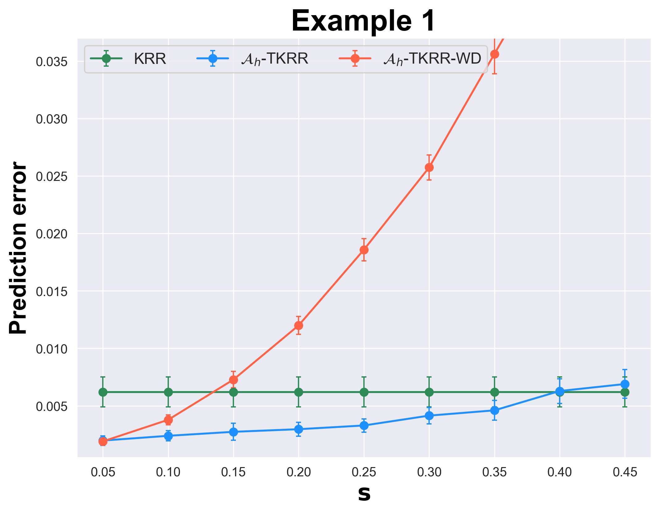
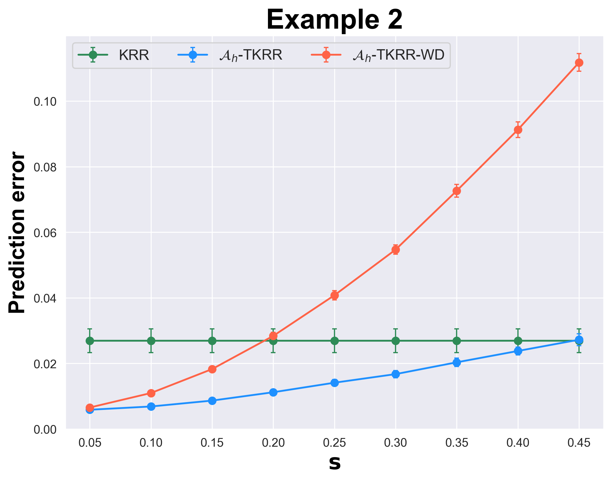
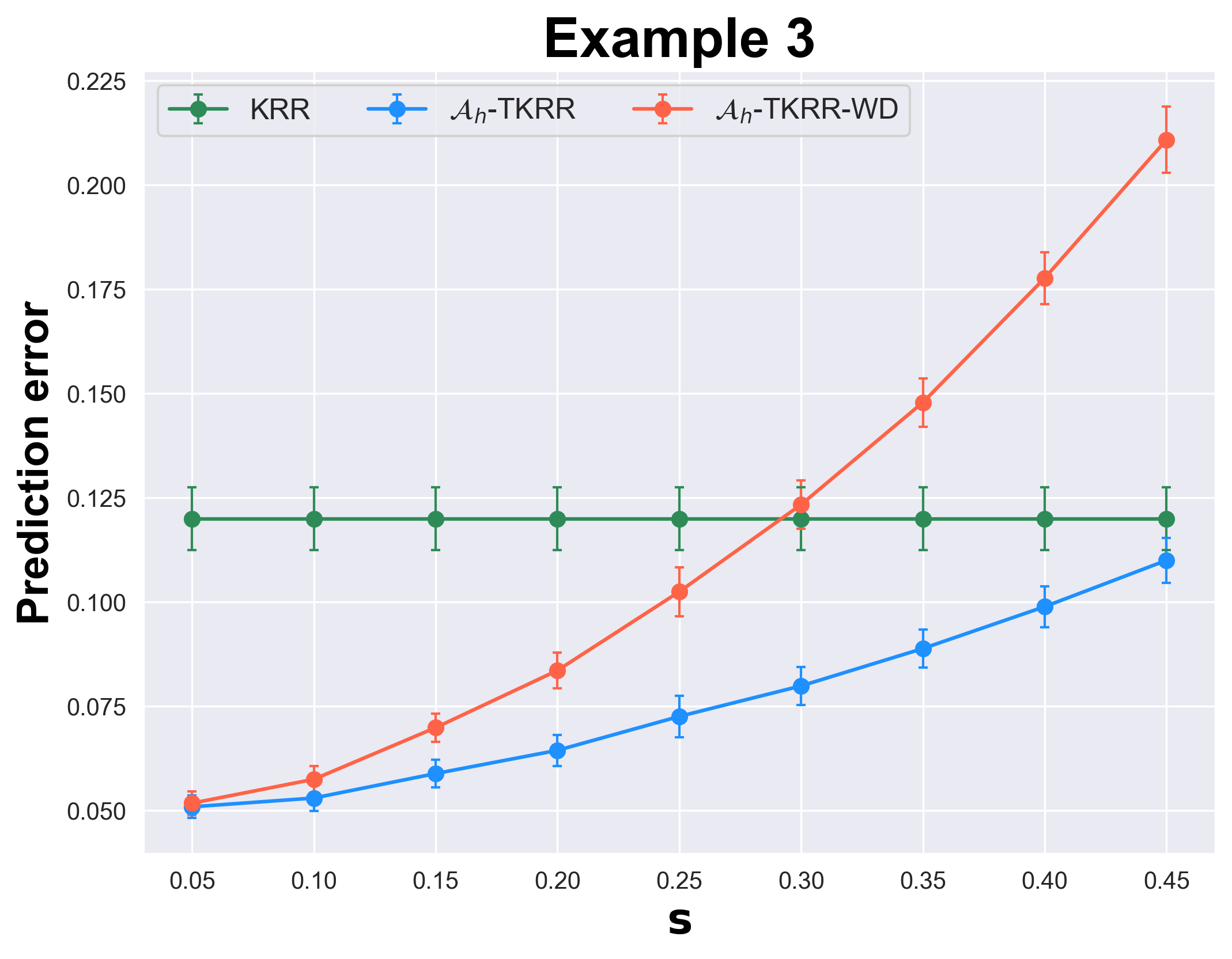
Figure 3: Prediction errors of all the competitors in Examples 1–3 with varying $s$.

Example 3. The generating scheme is exactly the same as Example 2 except that ${\mathop{\bf x}}_{i}^{(k)}=(x^{(k)}_{1i},\ldots,x^{(k)}_{10i})^{\top}\in\mathbb{R}^{10}$ and $f^{(k)}_{\rho}$ has the form that

$$f^{(k)}_{\rho}({\mathop{\bf x}}_{i}^{(k)})=\sin(0.75\pi w_{1i}^{(k)})+3|w_{2i}^{(k)}-s^{(k)}-0.5|-e^{w_{3i}^{(k)}}$$

with $w_{1i}^{(k)}=x^{(k)}_{1i}+x^{(k)}_{4i}+x^{(k)}_{5i}+x^{(k)}_{6i},w_{2i}^{(k)}=(x^{(k)}_{1i}+x^{(k)}_{2i}+x^{(k)}_{3i})/3,w_{3i}^{(k)}=(x^{(k)}_{6i})^{2}+(x^{(k)}_{7i})^{2}-(x^{(k)}_{8i})^{2}-(x^{(k)}_{9i})^{2}$.

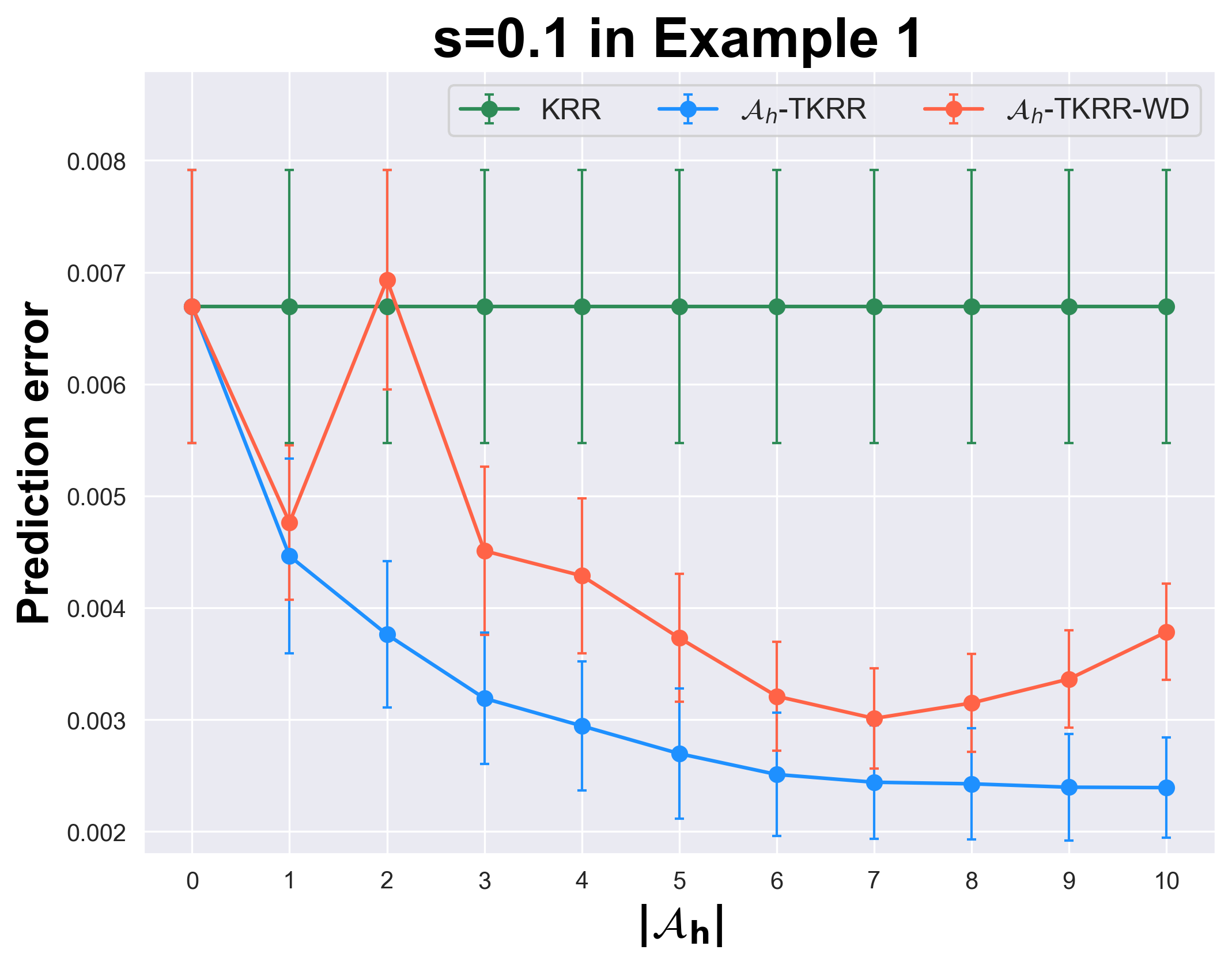
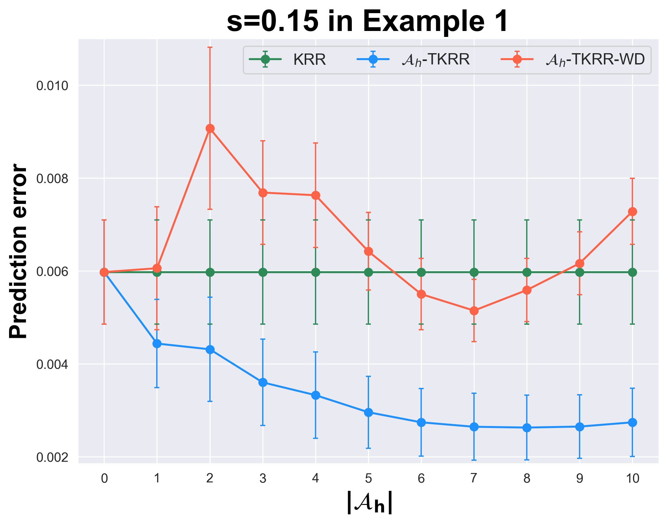
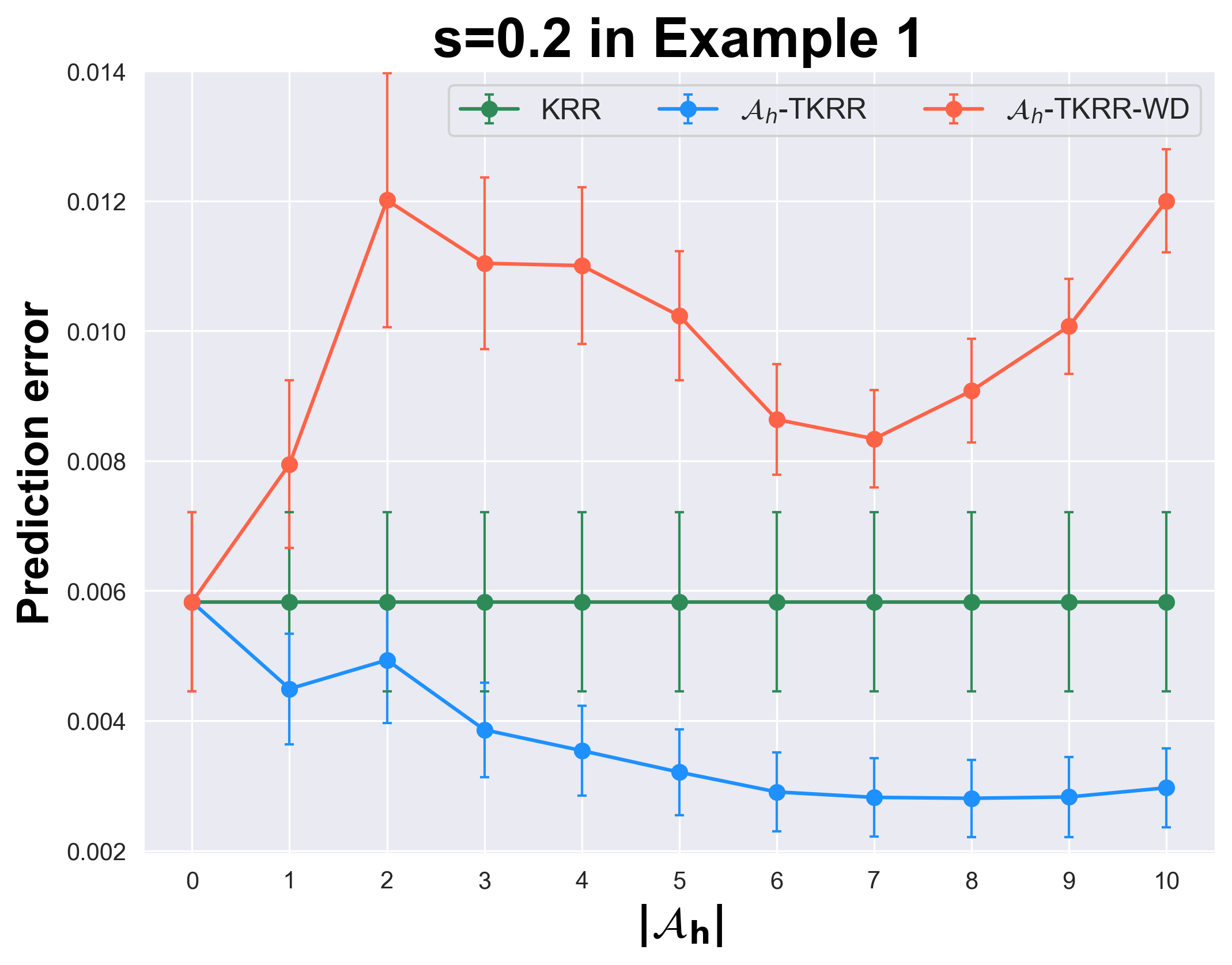
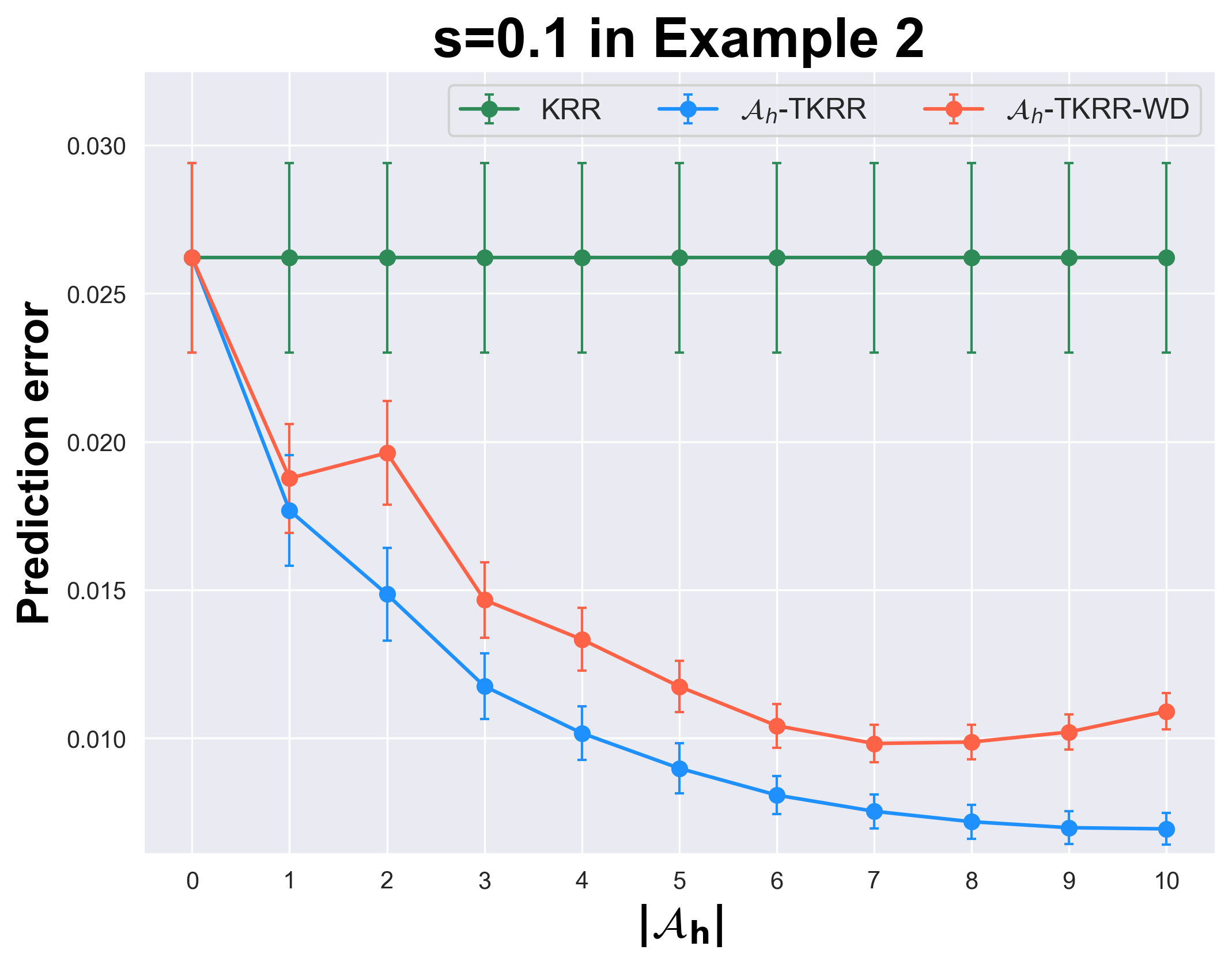
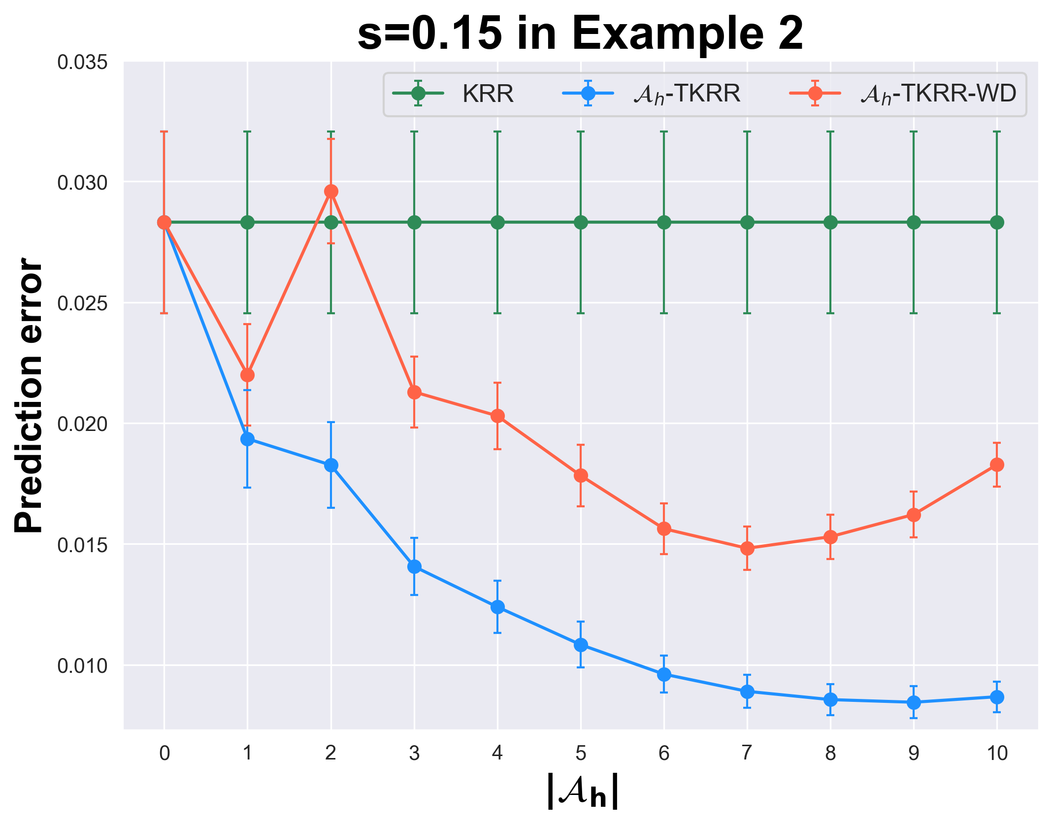
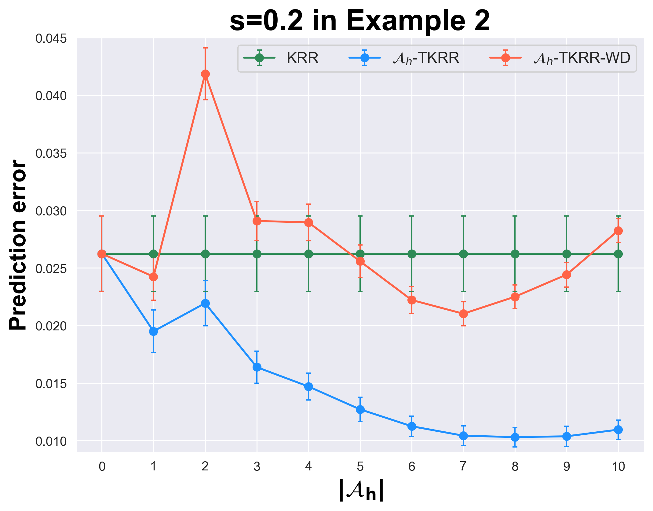
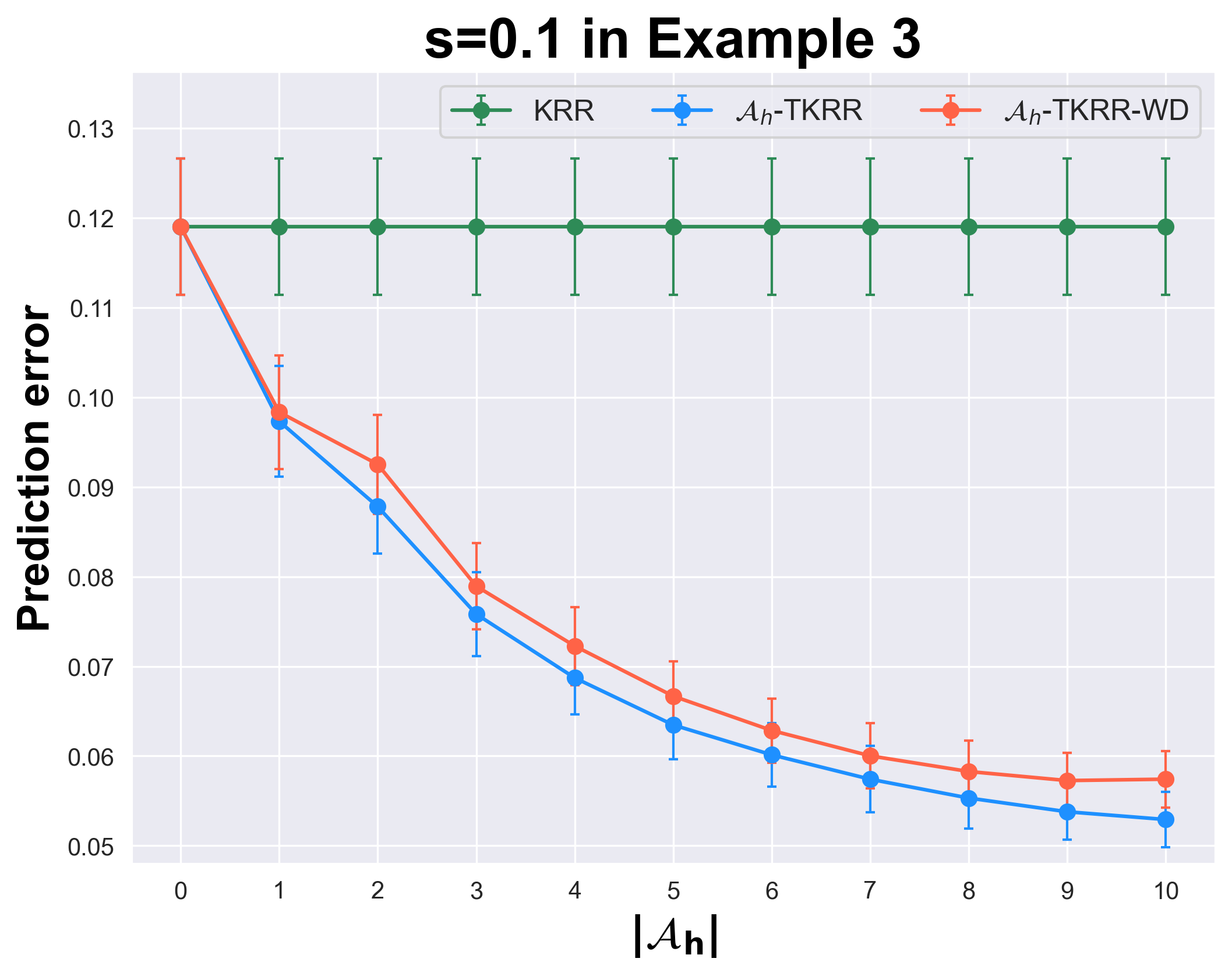
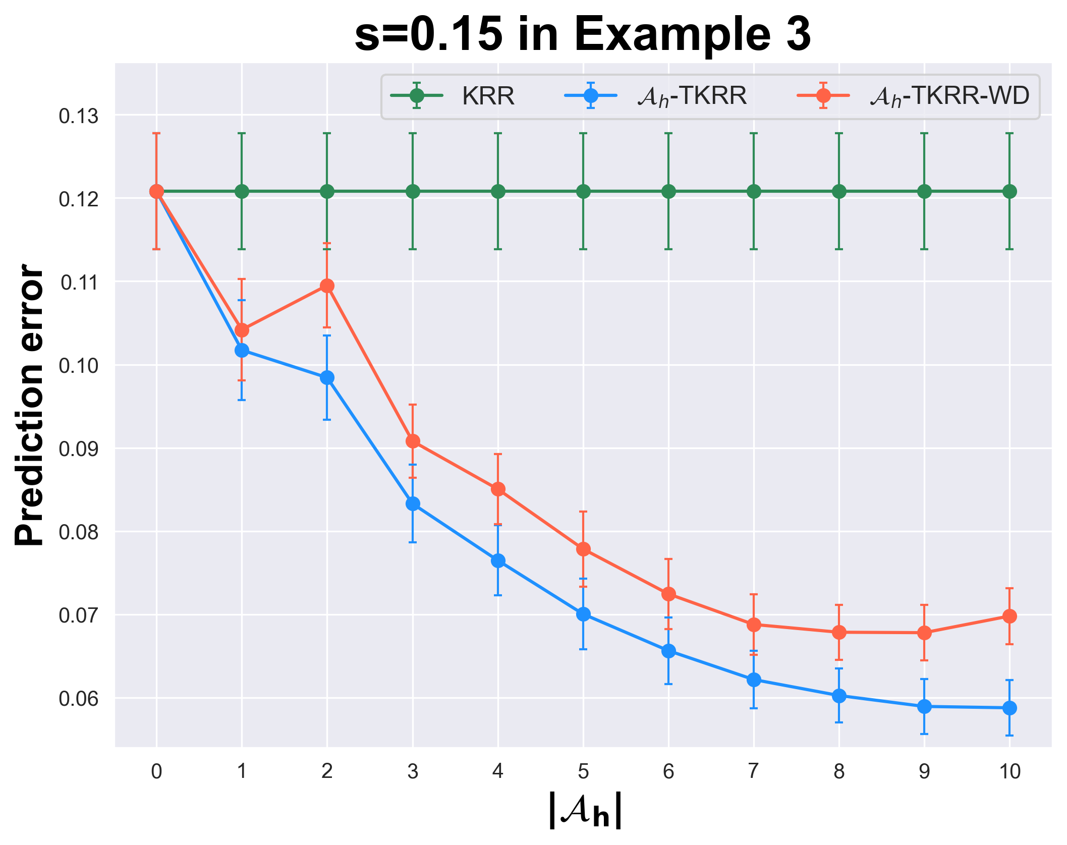
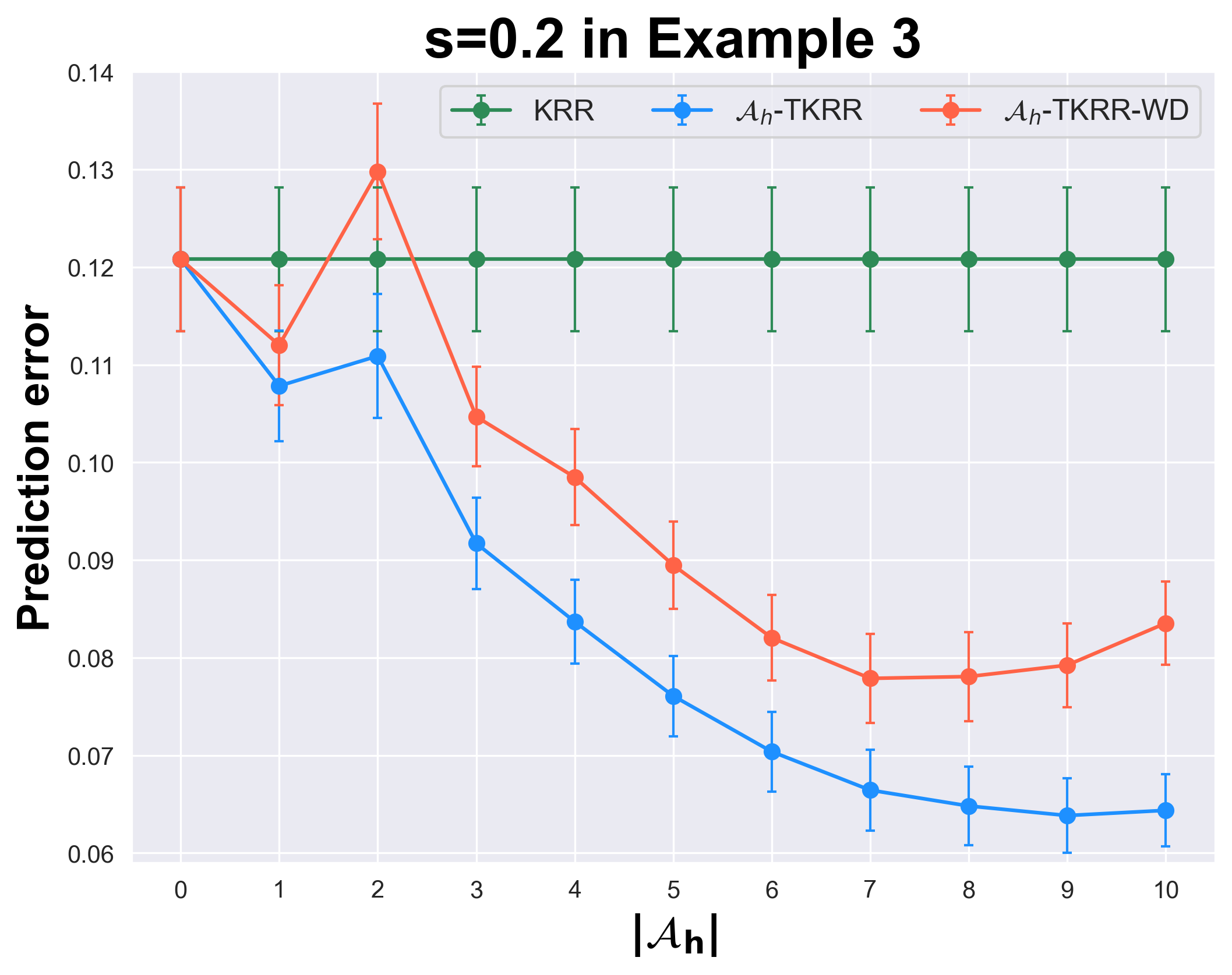
Figure 4: Prediction errors of all the competitors in Examples 1–3 under various scenarios with varying $|{\cal A}_{h}|$.

It is thus clear that the scalar covariate is used in Example 1, and the multi-dimensional covariates are considered in Examples 2 and 3. In all the numerical experiments, unless specified otherwise, we set $n_{0}=200$ and $n_{k}=150$ for each $k$ in Example 1 and set $n_{0}=600$ and $n_{k}=300$ for each $k$ in both Examples 2 and 3. To comprehend the effect of the similarity parameter $s$, we apply all the competitors to Examples 1–3 and vary $s$ from $\{0.05,0.10,\ldots,0.45\}$. Moreover, we assume that all the sources are known to be transferable in the sense that ${\cal A}_{h}=\{1,2,\ldots,10\}$. It is worth pointing out that since we assume that all the sources are transferable, and thus the similarity level $h$ increases with the increasing of $s$. Each of the scenarios is replicated 100 times and the averaged performance of all the competitors is evaluated by the prediction error of the estimator $\widehat{f}$ that $\|\widehat{f}-f_{\rho}\|_{n}^{2}=\frac{1}{n_{te}}\sum_{i=1}^{n_{te}}(\widehat{f}({\mathop{\bf x}}_{i})-f_{\rho}^{(0)}({\mathop{\bf x}}_{i}))^{2}$ with a new testing dataset drawn from the target model with $n_{te}=500$. Figure 3 shows the prediction performance of all the competitors with different choices of $s$.

It is thus clear from Figure 3 that ${\cal A}_{h}$-TKRR outperforms KRR and ${\cal A}_{h}$-TKRR-WD for almost all the scenarios. Specifically, when $s$ is small, the target model and the source models are closely related, and thus the source data can provide sufficient information for transfer learning the target model. This leads to significant numerical improvement of ${\cal A}_{h}$-TKRR compared to the performance of KRR. With the increasing of $s$, the performance of ${\cal A}_{h}$-TKRR tends to coincide with that of KRR, which is due to the fact that the differences between the target model and the source models become larger, and thus the source data can not provide much information. These observations match our theoretical findings in Theorem 1 that the upper bound of the prediction error is proportional to $h^{\frac{\alpha}{1+\alpha}}$ which is positively related to $s$. It is also interesting to notice that ${\cal A}_{h}$-TKRR always outperforms ${\cal A}_{h}$-TKRR-WD in all the scenarios, which indicates the necessity of the adopted debiasing step.

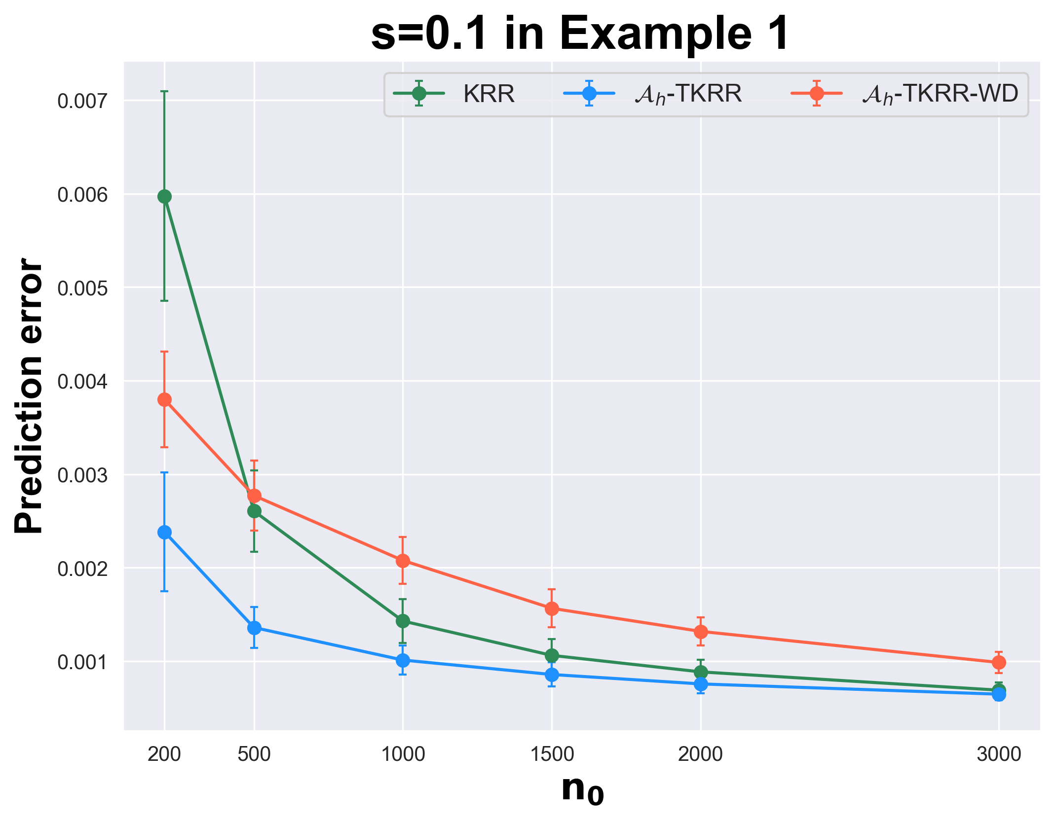
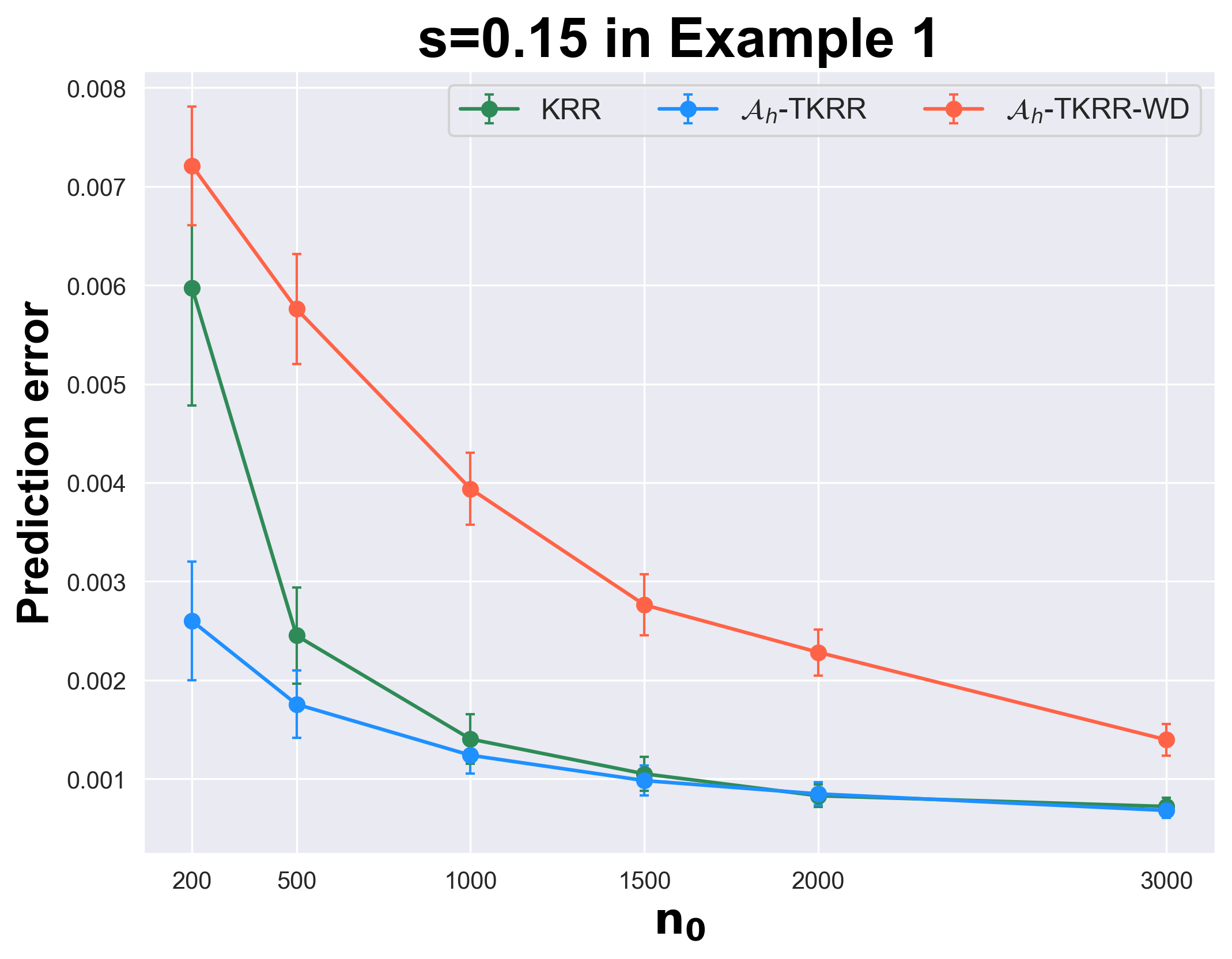
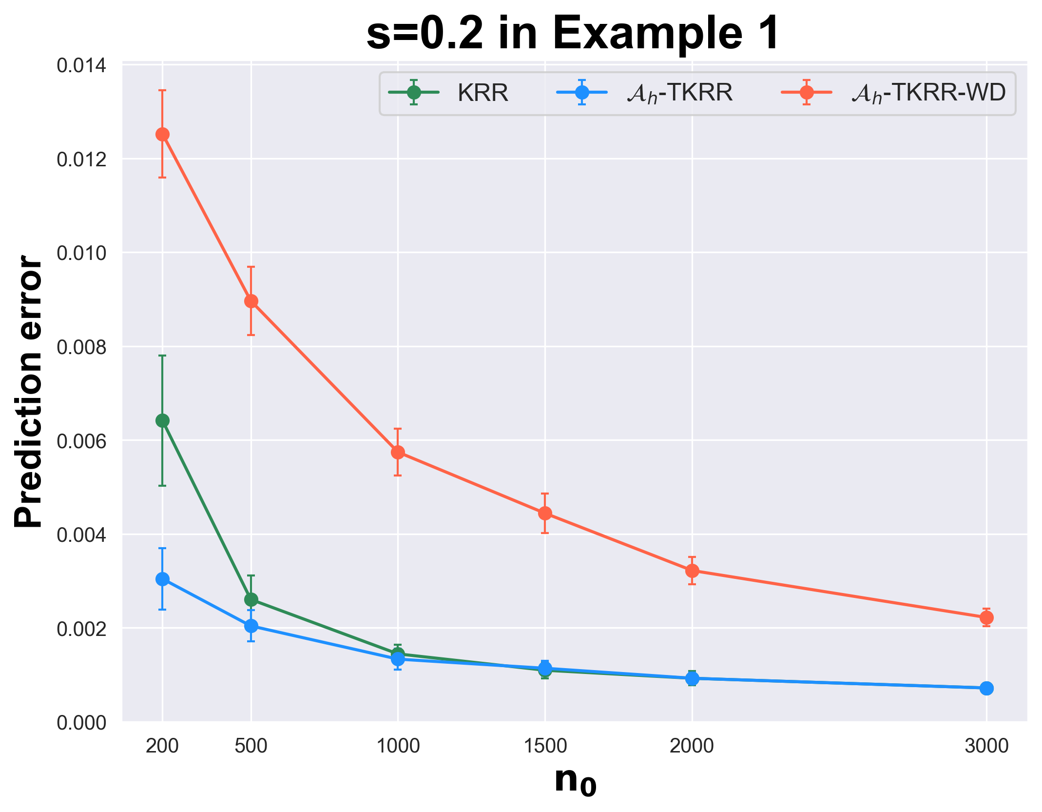
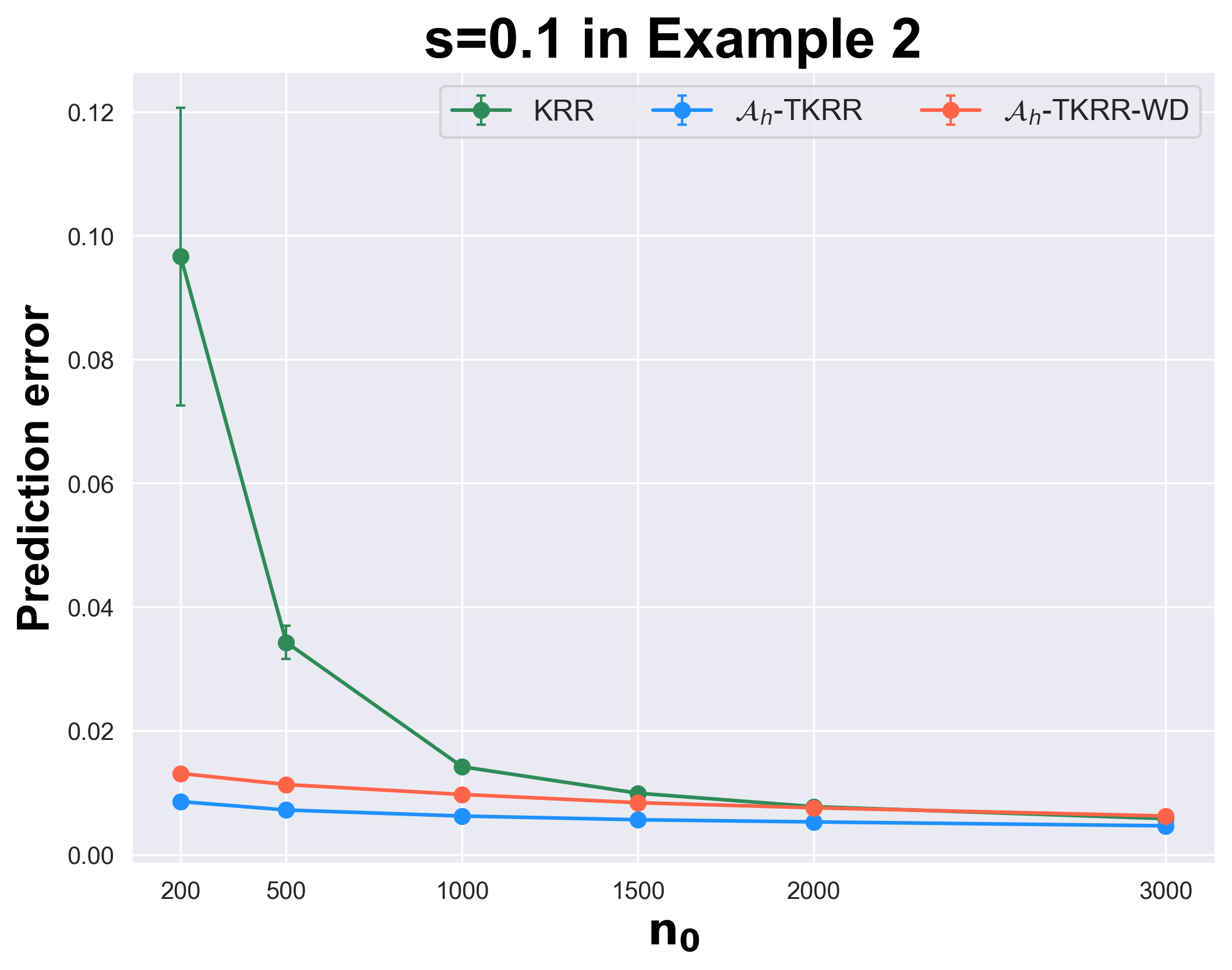
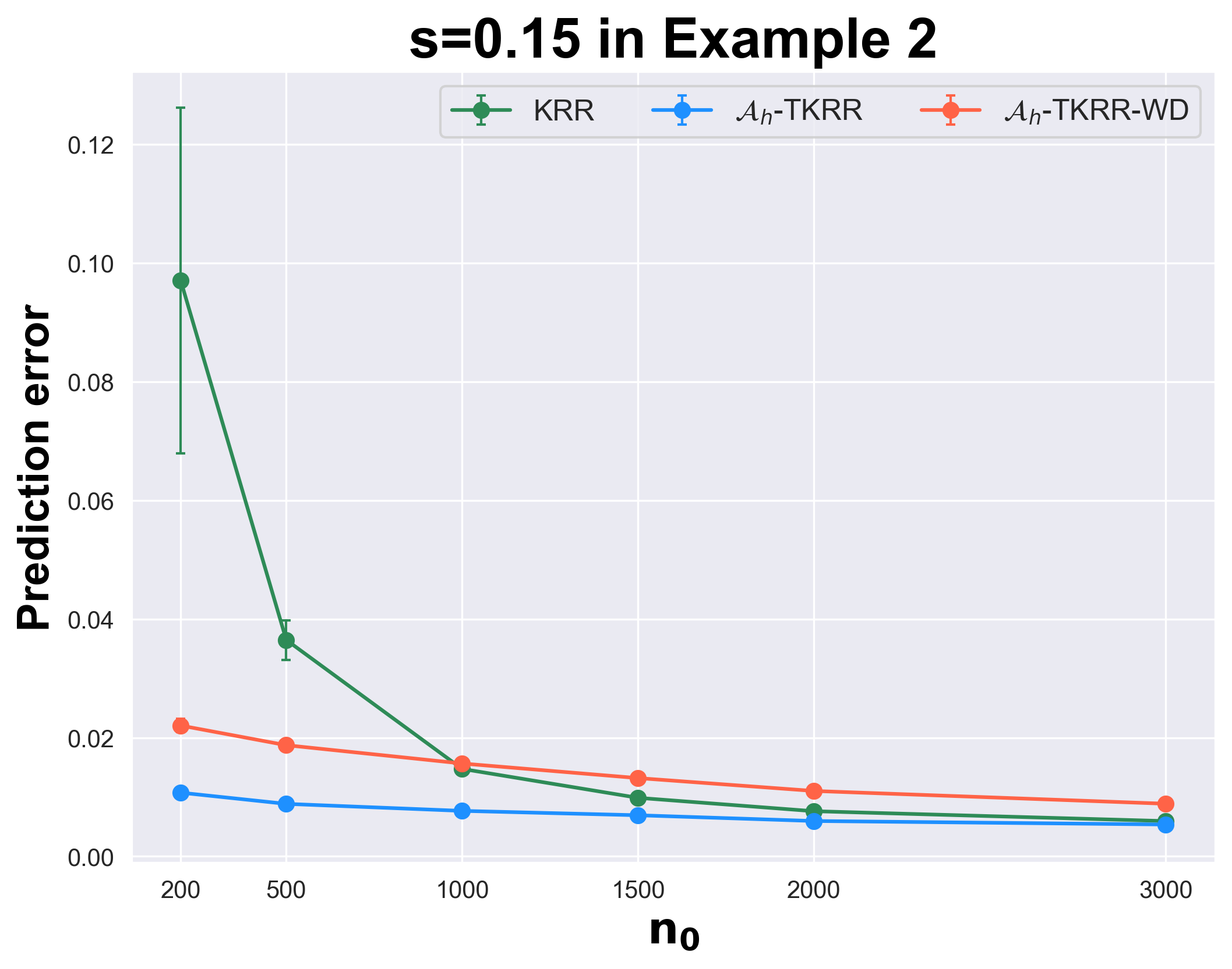
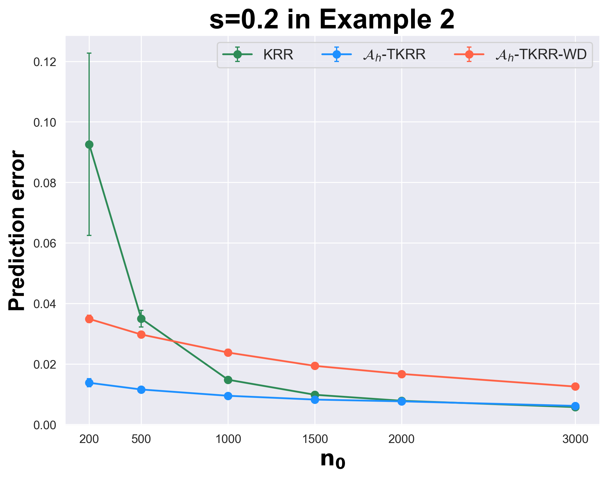
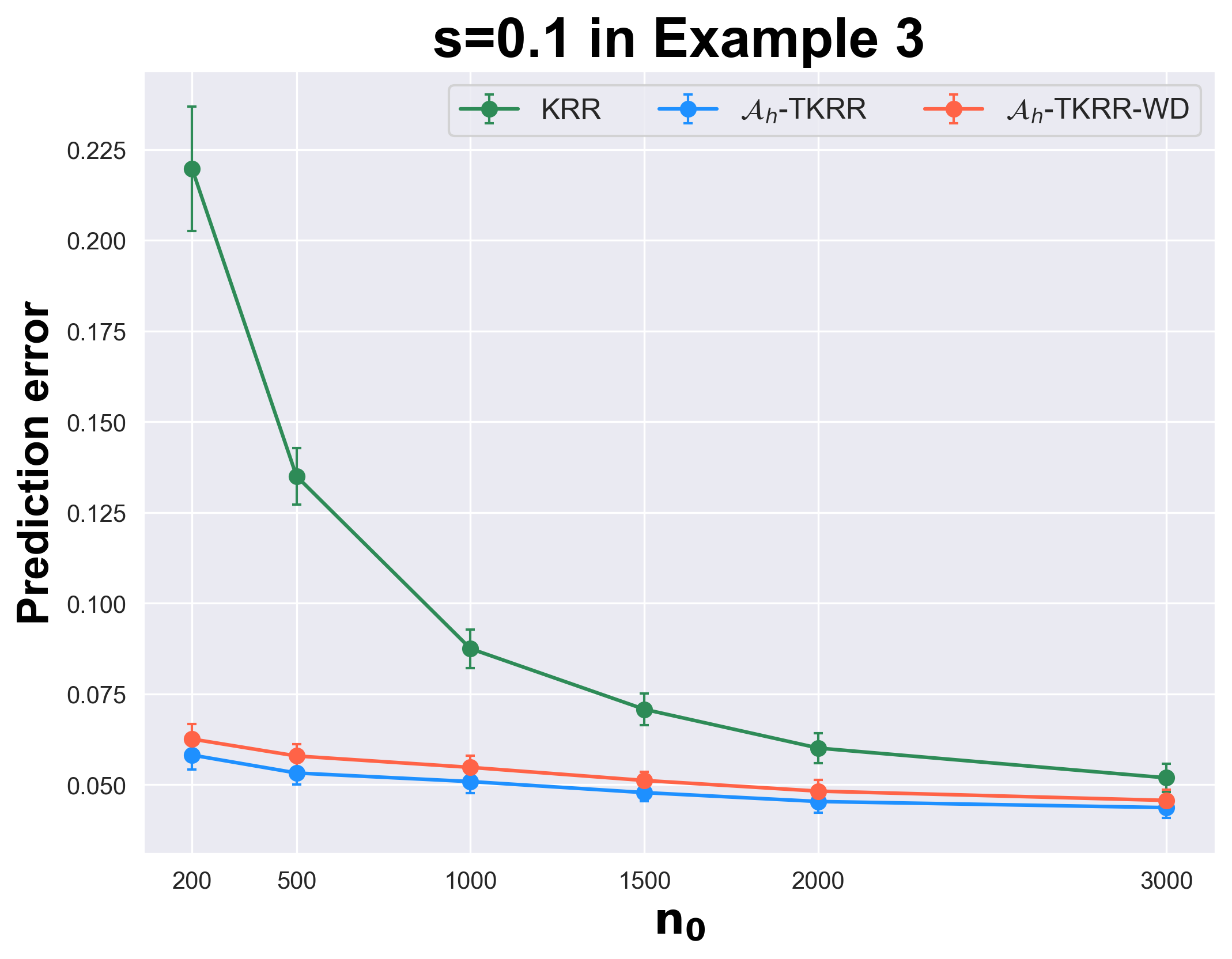
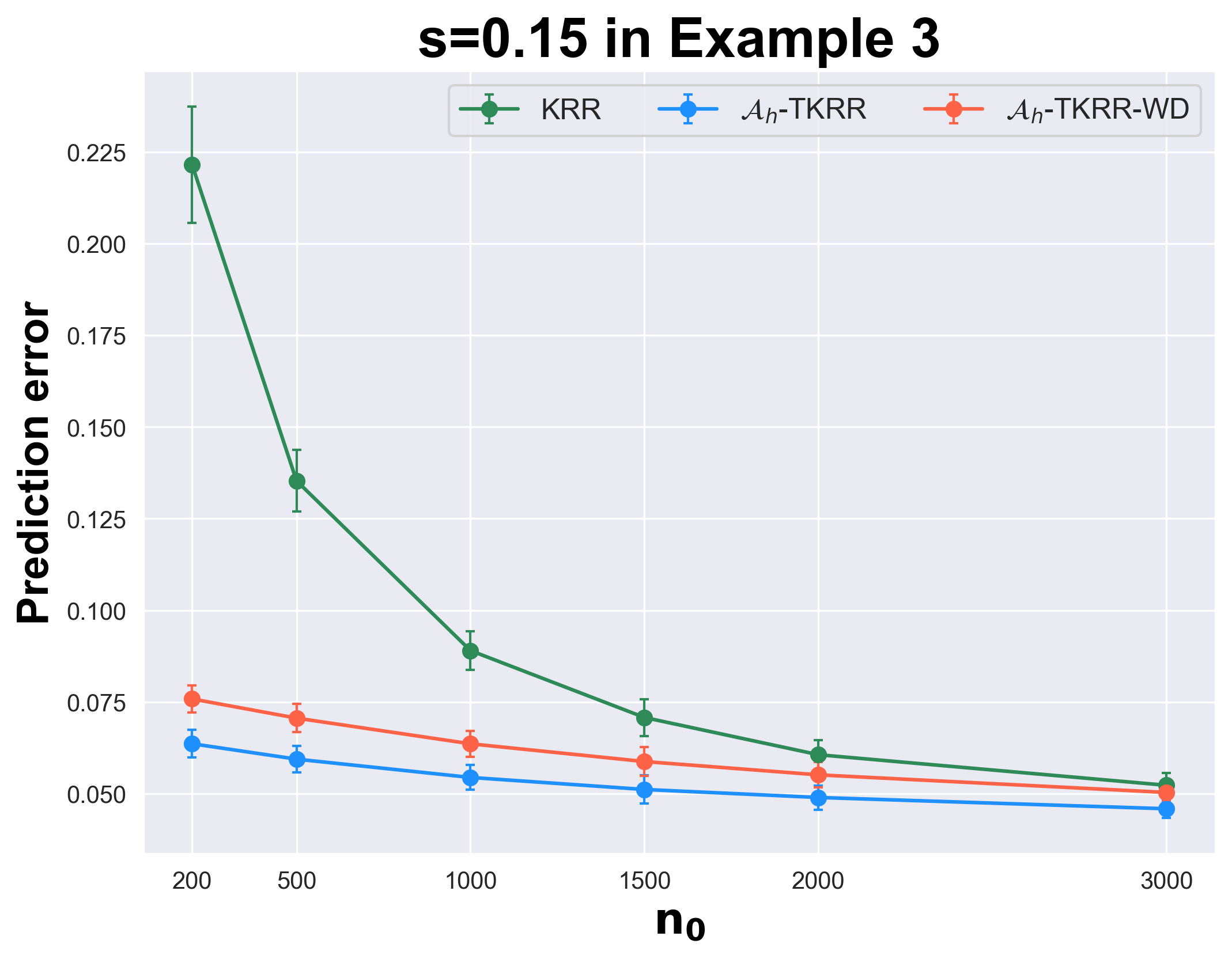
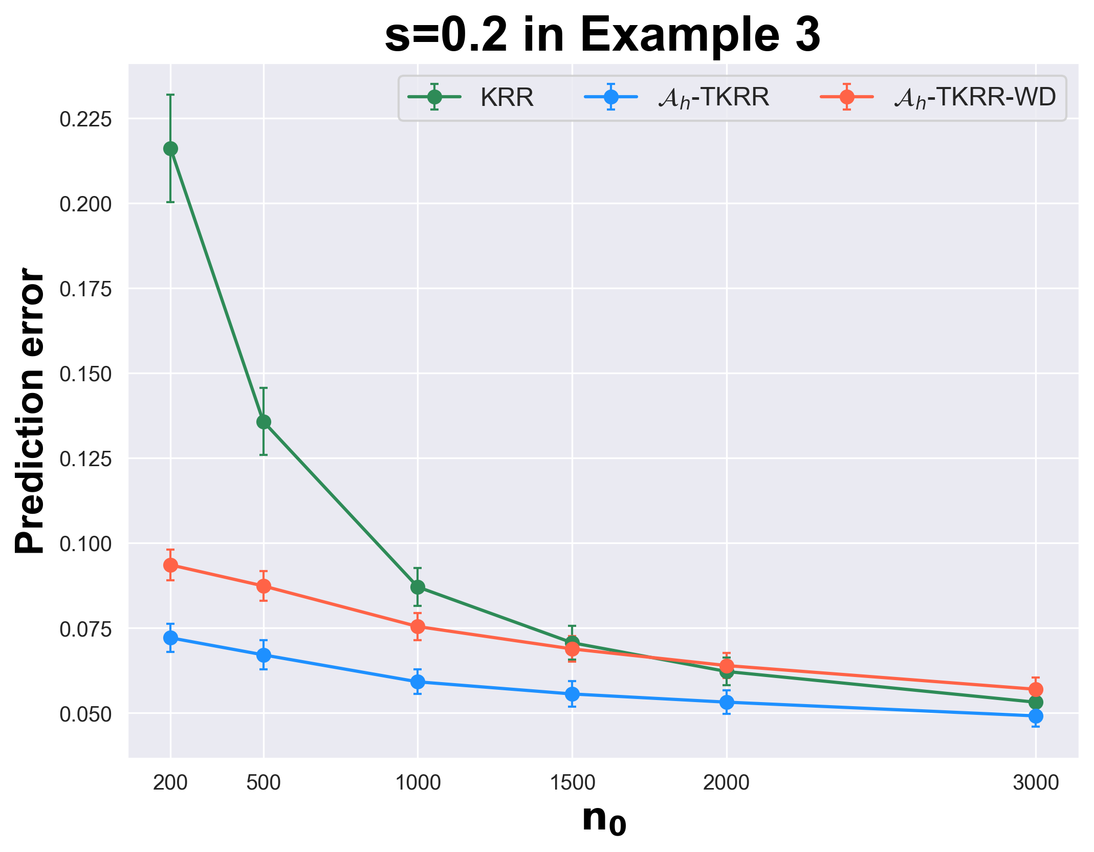
Figure 5: Prediction errors of all the competitors in Examples 1–3 under various scenarios with varying $n_{0}$.

We also investigate how the performance of ${\cal A}_{h}$-TKRR is affected by the number of sources. Specifically, we apply all the competitors to Examples 1–3 and vary $|{\cal A}_{h}|$ from $\{0,1,\ldots,10\}$ in the sense that ${\cal A}_{h}=\{1,\ldots,|{\cal A}_{h}|\}$ for $|{\cal A}_{h}|>0$ and $s$ from $\{0.10,0.15,0.20\}$. Each of the scenarios is replicated 100 times and the averaged performance of all the competitors is evaluated by the prediction error, which is summarized in Figure 4. From Figure 4, we observe that ${\cal A}_{h}$-TKRR outperforms KRR and ${\cal A}_{h}$-TKRR-WD in all the scenarios where $|{\cal A}_{h}|>0$. This indicates that the source data can contribute to the transfer learning of the target model, and the debiased step further improves the learning accuracy. Moreover, in all the scenarios, the prediction error of ${\cal A}_{h}$-TKRR decreases as $|{\cal A}_{h}|$ grows at first, and then flattens out, which closely coincides with the results in Theorem 1. It is also worthnoting that for the larger $s$, the curves of ${\cal A}_{h}$-TKRR flatten out earlier, which is also consistent with our theoretical findings.

To investigate the effect of the target sample size $n_{0}$, we apply all the competitors to Examples 1–3 and vary $n_{0}$ from $\{200,500,1000,1500,2000,3000\}$ and $s$ from $\{0.1,0.15,0.2\}$. We also assume that all the sources are transferable that ${\cal A}_{h}=\{1,2,\ldots,10\}$. Each of the scenarios is replicated 100 times and the averaged performance of all the competitors is evaluated by the prediction error as illustrated in Figure 5. From Figure 5, it is clear that when $n_{0}$ is sufficiently large, the numerical performance of ${\cal A}_{h}$-TKRR is similar to that of KRR. Yet, with the decreasing of $n_{0}$, the advantage of ${\cal A}_{h}$-TKRR becomes more and more obvious. Moreover, the curves of ${\cal A}_{h}$-TKRR-WD have some significant gaps with those of ${\cal A}_{h}$-TKRR, which further indicates that the debiasing step is necessary in practice.

5.2 Transfer KRR When ${\cal A}_{h}$ is Unknown

In Section 5.1, we assume that the transferable sources are known, yet such prior information may not be available in practice. In this part, we evaluate the numerical performance of SA-TKRR proposed in Section 3.2 and compare it to some state-of-the-art competitors, including KRR where only the target data is used, Pooled-TKRR where Algorithm 1 is implemented with all sources, D-TKRR where Algorithm 1 is implemented with the detection procedure used in Tian & Feng (2022) and AEW-TKRR where Algorithm 2 is implemented using exponential weight aggregation Leung & Barron (2006) without the re-train step.

Specifically, we consider the multi-dimensional cases and assume that the number of the sources is $m+3$. Specifically, the data generating schemes are the same as Examples 2 and 3 in Section 5.1 except that for the last 3 sources, $s^{(m+1)},s^{(m+2)},s^{(m+3)}$ are independently drawn from $U(s,0.4)$, and we denote these examples as modified Example 2 and 3, respectively. Note that ${\cal A}_{h}$ is unknown, and thus we apply SA-TKRR and all the other competitors to Examples 2 and 3 and vary $m$ from $\{0,1,2,\ldots,10\}$ and $s$ from $\{0.2,0.25,0.3\}$. Each of the scenarios is replicated 100 times and the averaged performance of all the competitors is evaluated by the prediction error presented in Figure 6.

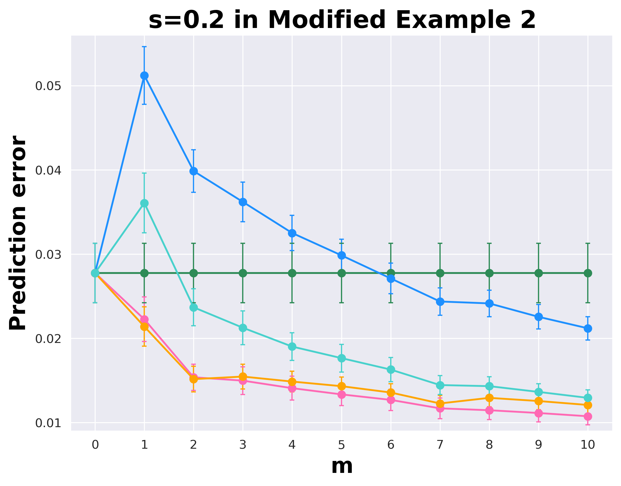
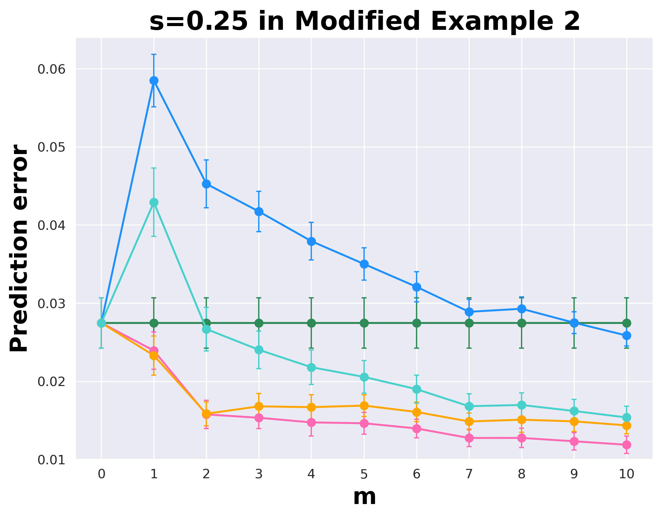
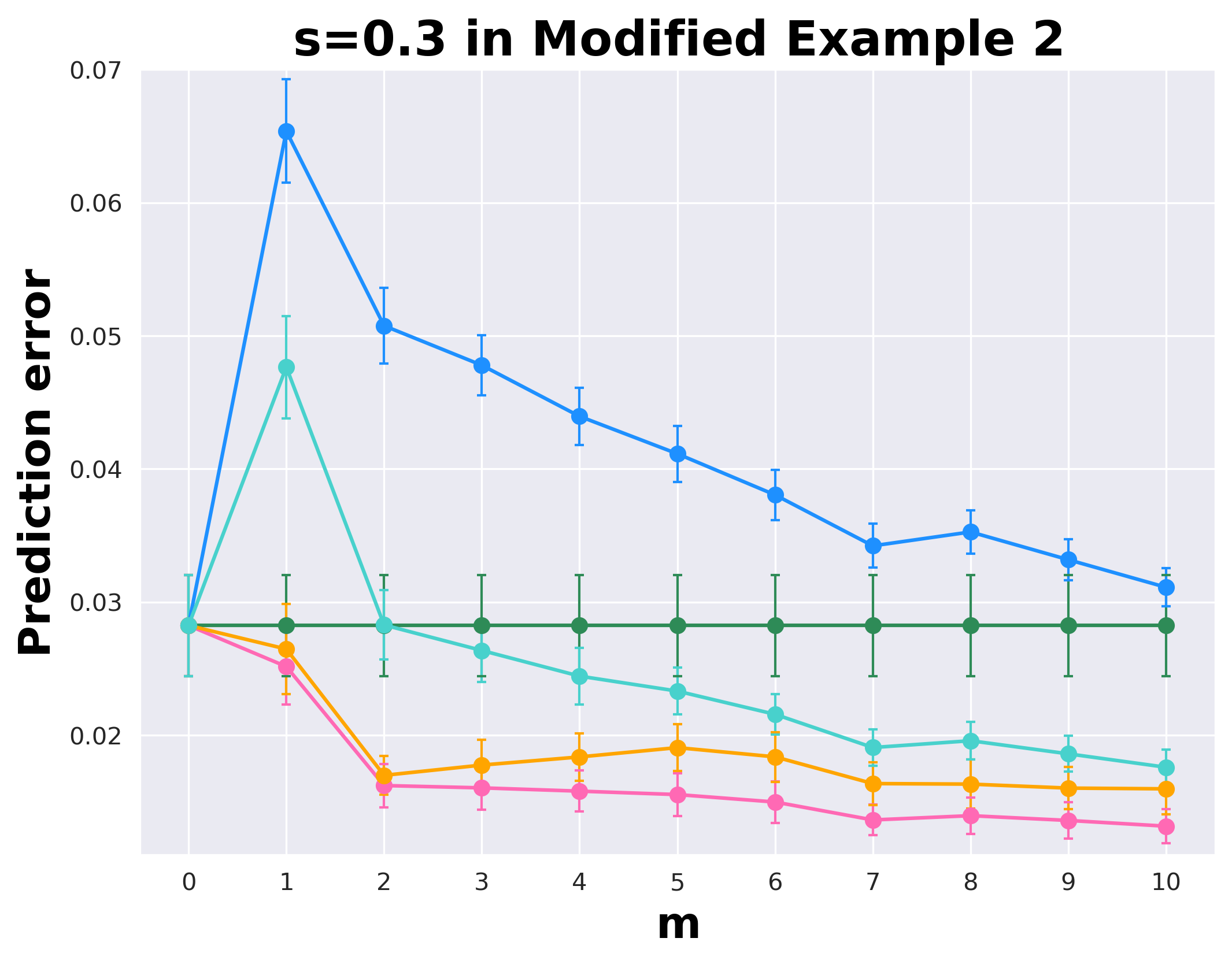
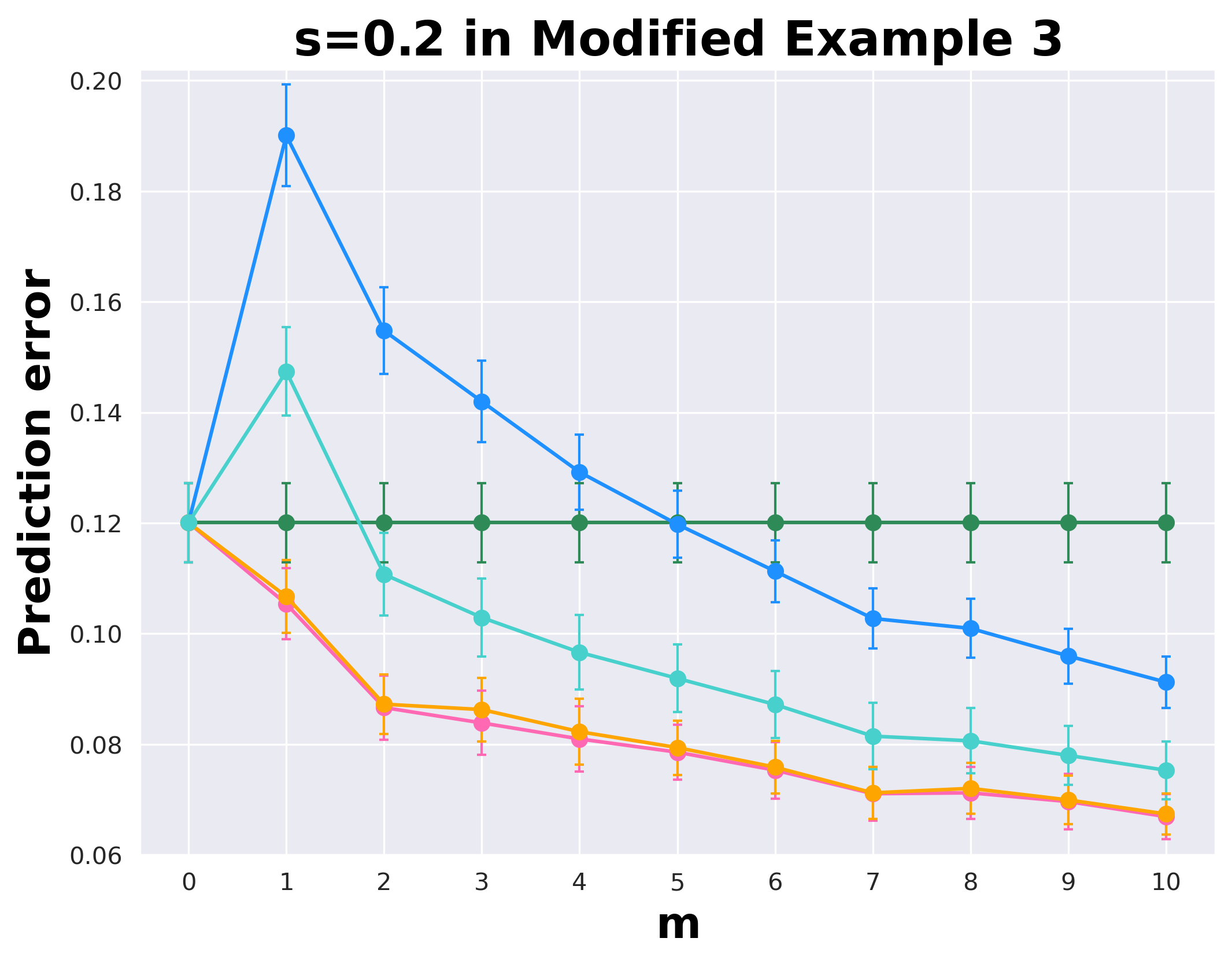
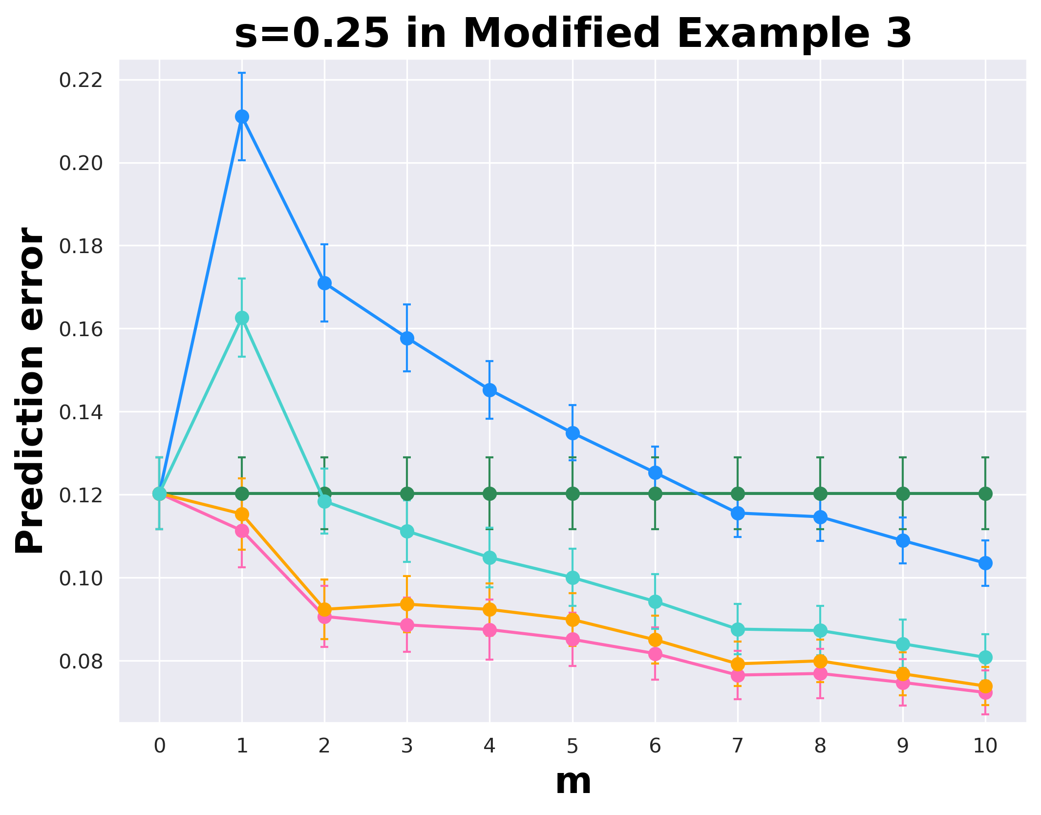
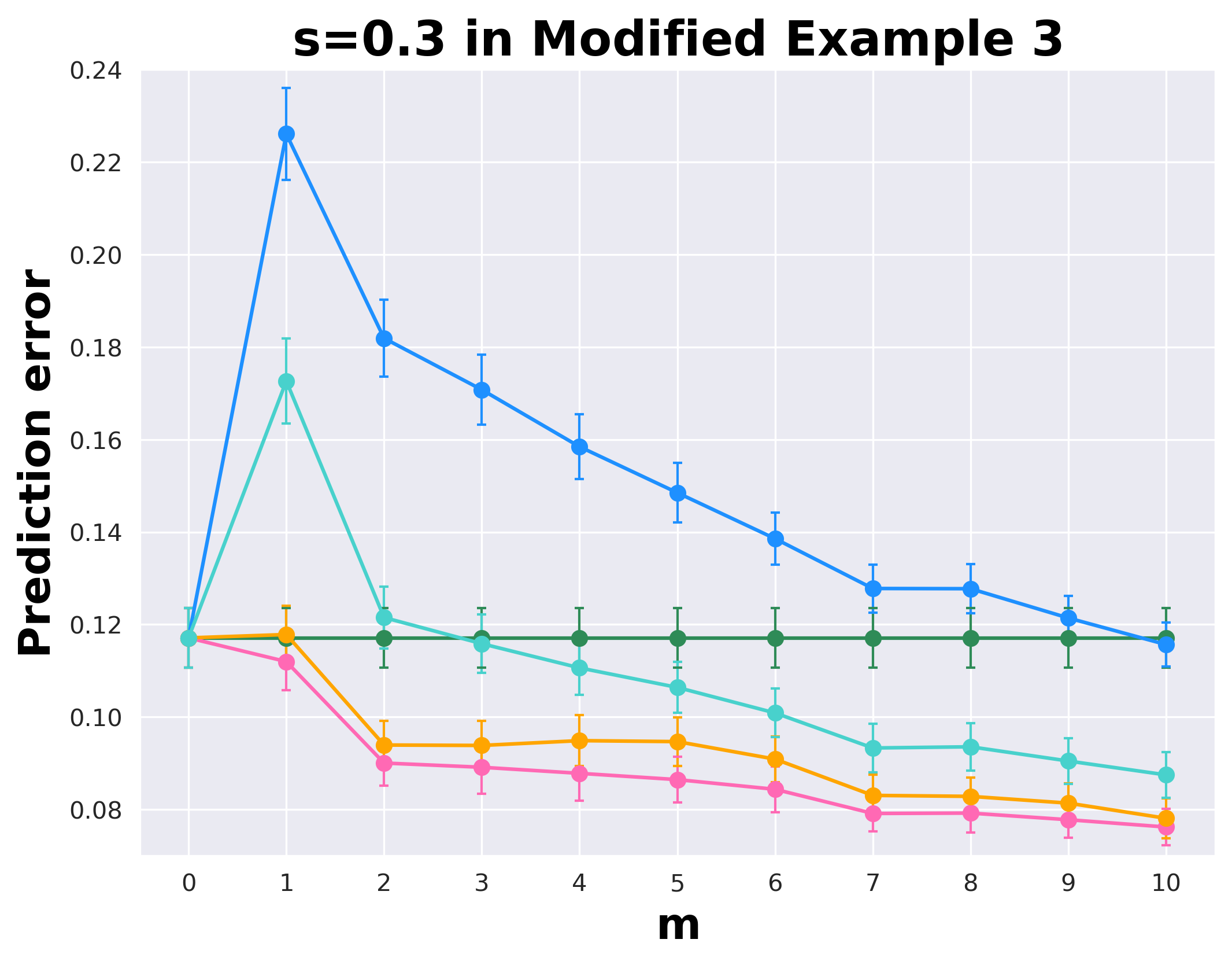
Figure 6: Prediction errors of all the competitors in modified Examples 2 and 3 under various scenarios with varying $m$.

It is thus clear from Figure 6 that SA-TKRR outperforms all the other competitors in almost all the scenarios, which indicates the effectiveness of SA-TKRR in not only capturing useful information contained in the source data but also mitigating the impact of negative sources. This observation also supports our theoretical findings in Section 4.2. It is worthy pointing out that the prediction performance of Pooled-TKRR is even worse than KRR in most settings, which indicates that simple transfer learning with all the sources data is not preferable since the existing negative sources can bring harmful impact. The performance of AEW-TKRR is less satisfactory especially when $m$ is relatively small, which is largely due to its required target data splitting procedure. Note that although the performance of D-TKRR is close to that of SA-TKRR, it is much more computationally challenging due to the adopted detection procedure.

6 Real Data Analysis

In this section, we apply the proposed algorithms to two real applications, where we consider the single source case with known ${\cal A}_{h}$ in the first application and the multiple source case with unknown ${\cal A}_{h}$ in the second application. In both examples, we follow the same treatment as those in Section 5 for the choices of RKHS, tuning parameters, and we report the prediction error of the response on the test data, where $f_{\rho}^{(0)}({\mathop{\bf x}}_{i})$ is replaced by $y_{i}$ that $\frac{1}{n_{te}}\sum_{i=1}^{n_{te}}(\widehat{f}({\mathop{\bf x}}_{i})-y_{i})^{2}$.

6.1 Wine Quality Data

In this part, a real application to the Portuguese Vinho Verde wine data (Cortez et al., 2009) is considered, which is available in http://www3.dsi.uminho.pt/pcortez/wine/. This dataset contains the qualities of red and white wines and consists of the response (wine quality) and 13 covariates, including fixed acidity, citric acid and alcohol. Note that the two types of wines share the same covariates but the underlying model may not be the same, and thus it is reasonable to consider transfer learning. Following the same treatment as that in Cai & Pu (2023), we use the white wine samples as the source data and the red wine samples as the target data, and the sample sizes are 4898 and 1599, respectively. Then, the primary interest is to enhance the prediction accuracy of the red wine quality with the help of the white wine data.

In this application, ${\cal A}_{h}$ is known and only contains one source data, and thus we apply ${\cal A}_{h}$-TKRR to this data and compare its performance to that of KRR and ${\cal A}_{h}$-TKRR-WD. Following the similar treatment as that in Cai & Pu (2023), we adopt random forest (Breiman, 2001) to rank the feature importance and select the first three influential features: ‘alcohol’, ‘sulfates’, and ‘volatile acidity’ for modeling. We are interested in the performance of the competitors in various scenarios with varying $n_{0}$ and $n_{{\cal A}_{h}}$. To be specific, we randomly select samples with size $n_{{\cal A}_{h}}$ and $n_{0}$ from the source and target data, respectively, and vary $n_{{\cal A}_{h}}$ from $\{0,200,400,600,800,1000,1500\}$ and $n_{0}$ from $\{100,200,300\}$. We use all the remaining samples in the target data to evaluate the prediction accuracy. Each scenario is replicated 100 times and the averaged numerical performance is illustrated in Figure 7.

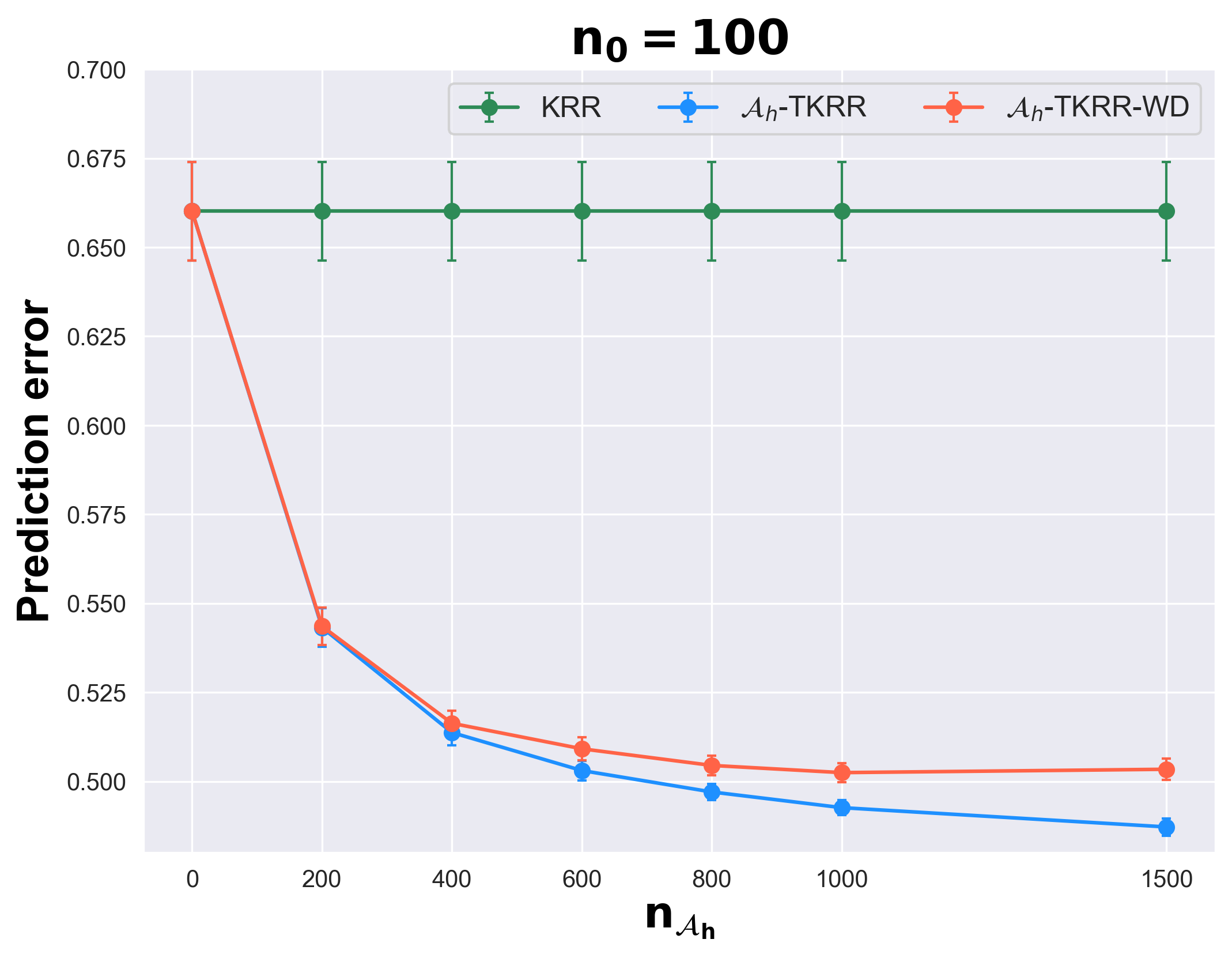
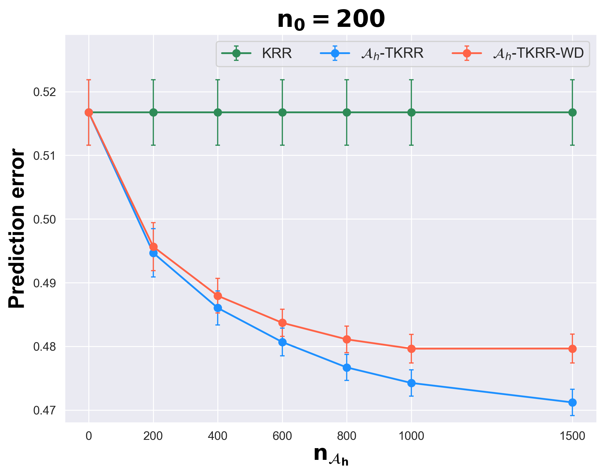
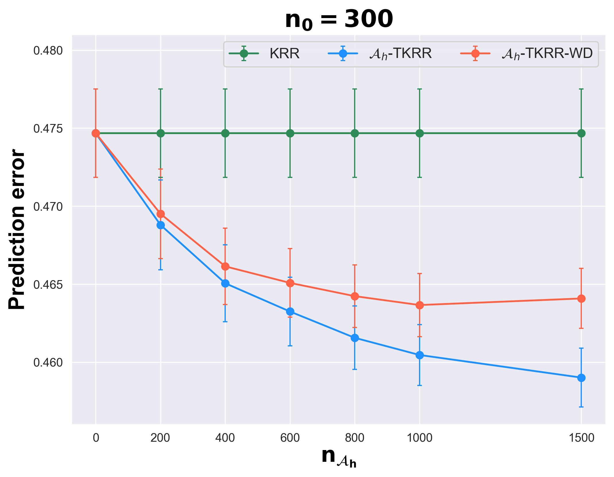
Figure 7: Prediction errors of all the competitors under various scenarios in the wine quality data.

From Figure 7, we can conclude that ${\cal A}_{h}$-TKRR outperforms the other two methods in all the scenarios. This demonstrates the prediction performance of the red wine quality can be significantly improved by utilizing the source data. It is also interesting to notice that the prediction error of ${\cal A}_{h}$-TKRR decreases with the increasing of $n_{{\cal A}_{h}}$ and is much smaller than that of ${\cal A}_{h}$-TKRR-WD, which further verifies that the prediction enhancement is not simply due to the larger sample size, but also the effectiveness of transfer learning.

6.2 UK Used Car Data

In this subsection, a real application to the UK used car price data is considered which is available in https://www.kaggle.com/datasets/kukuroo3/used-car-price-dataset-competition-format. This dataset comprises information from nine popular car brands in the UK market: Mercedes Benz (Merc), Ford, Volkswagen (VW), Bayerische Motoren Werke (BMW), Hyundai, Toyota, Skoda, Audi, and Vauxhall, and the sample sizes of each car brand are $1219,1196,$ $1159,978,817,717,638,523$ and $385$, respectively. The response variable is the price of each used car, and the covariates consist of crucial details about the used cars, such as registration year, mileage, road tax, miles per gallon (mpg), engine size, type of gearbox, and fuel type. The primary interest of this application is to predict the used car prices for some specific car brand to assist the seller for determining the optimal selling time, and thus we adopt transfer learning to enhance the prediction accuracy of one target car brand by utilizing the information of other car brands.

Specifically, we sequentially treat the samples of each car brand as the target data and all the samples of the other car brands are the source data. For each target data, we randomly select half of them for training and use the rest of them to evaluate the prediction accuracy. Note that in this application, we don’t have any prior information on which source is transferable, and thus SA-TKRR is adopted. Moreover, we compare the performance of SA-TKRR to the methods considered in Section 5.2, including KRR, Pooled-TKRR, AEW-TKRR, and D-TKRR. Each case is replicated 100 times and the averaged numerical performance is summarized in Table 1.

Table 1: Prediction errors of all the competitors in the UK used car data together with their standard errors in parentheses.

Methods	Target Brands
	Merc	Ford	VW	BMW	Hyundai	Toyota	Skoda	Audi	Vauxhall
SA-TKRR	0.4918	0.0596	0.1746	0.6686	0.0259	0.1211	0.0221	0.5364	0.0333
	(0.127)	(0.015)	(0.014)	(0.145)	(0.005)	(0.024)	(0.002)	(0.219)	(0.008)
KRR	0.5176	0.0623	0.1838	0.7179	0.0297	0.1562	0.0251	0.7327	0.0413
	(0.138)	(0.012)	(0.013)	(0.151)	(0.007)	(0.040)	(0.004)	(0.258)	(0.010)
Pooled-TKRR	0.5109	0.0710	0.1723	0.6733	0.0371	0.1150	0.0230	0.5396	0.0488
	(0.112)	(0.026)	(0.013)	(0.150)	(0.008)	(0.015)	(0.002)	(0.115)	(0.017)
AEW-TKRR	0.5698	0.0687	0.1971	0.7962	0.0386	0.1754	0.0246	0.7451	0.0532
	(0.123)	(0.014)	(0.018)	(0.185)	(0.012)	(0.036)	(0.002)	(0.228)	(0.019)
D-TKRR	0.5130	0.0639	0.1778	0.6695	0.0270	0.1169	0.0225	0.5460	0.0342
	(0.108 )	(0.023)	(0.014)	(0.152)	(0.006)	(0.020)	(0.002)	(0.118)	(0.006)

From Table 1, it is clear that SA-TKRR achieves the best prediction performance for all the brands except for VW and Toyota, which further illustrates the effectiveness of our proposed method. It is interesting to point out that Pooled-TKRR exhibits the leading performance for the brands VW and Toyota, and the performance of SA-TKRR is comparable to Pooled-TKRR. This is largely due to the fact that Vw and Toyota are very popular brands with many best-selling models, and thus they may exhibit more similarities with other brands, and thus all the source data become transferable. As opposed, to other brands that may share low similarities with others, pooling all the source data together may not be optimal due to the presence of negative sources.

7 Conclusion

This paper thoroughly investigates the transfer learning problem of KRR from both methodological and theoretical perspectives. Its primary objective is to bridge the gap between practical effectiveness and theoretical guarantees, addressing the fundamental question of whether the transfer estimation of KRR can achieve minimax optimality, which is of great interest to the machine learning community. To tackle the challenges, two highly efficient transfer learning methods are proposed, tailored to address scenarios where the transferable sources are either known or unknown. From a theoretical standpoint, this paper establishes the optimal minimax rate of the desired estimator in the known transferable sources case by utilizing various techniques in empirical process theory for analyzing kernel classes. Additionally, it demonstrates that the desired estimator in the unknown transferable source case can asymptotically approach the nearly optimal rate. Notably, this paper also sheds light on several intriguing directions for future research. One captivating avenue for future exploration is to theoretically understand the transfer learning problem in other kernel-based methods, such as kernel-based quantile regression and kernel support vector machines, which are also of significant interest to the machine learning community. We leave the pursuit of these promising research questions as future work.

References

- Bastani (2021) Bastani, H. (2021). Predicting with proxies: Transfer learning in high dimension. Management Science, 67, 2964–2984.
- Blitzer et al. (2007) Blitzer, J., Crammer, K., Kulesza, A., Pereira, F., & Wortman, J. (2007). Learning bounds for domain adaptation. Advances in Neural Information Processing Systems, 20, 129–136.
- Breiman (2001) Breiman, L. (2001). Random forests. Machine Learning, 45, 5–32.
- Cai & Pu (2023) Cai, T. T., & Pu, H. (2023). Transfer learning for nonparametric regression: Non-asymptotic minimax analysis and adaptive procedure. Manuscript, .
- Cai & Wei (2021) Cai, T. T., & Wei, H. (2021). Transfer learning for nonparametric classification: Minimax rate and adaptive classifier. The Annals of Statistics, 49, 100–128.
- Caponnetto & De Vito (2007) Caponnetto, A., & De Vito, E. (2007). Optimal rates for the regularized least-squares algorithm. Foundations of Computational Mathematics, 7, 331–368.
- Cortez et al. (2009) Cortez, P., Cerdeira, A., Almeida, F., Matos, T., & Reis, J. (2009). Modeling wine preferences by data mining from physicochemical properties. Decision Support Systems, 47, 547–553.
- Do & Ng (2005) Do, C. B., & Ng, A. Y. (2005). Transfer learning for text classification. Advances in Neural Information Processing Systems, 18, 299–306.
- Gaîffas & Lecué (2011) Gaîffas, S., & Lecué, G. (2011). Hyper-sparse optimal aggregation. The Journal of Machine Learning Research, 12, 1813–1833.
- Ge et al. (2014) Ge, L., Gao, J., Ngo, H., Li, K., & Zhang, A. (2014). On handling negative transfer and imbalanced distributions in multiple source transfer learning. Statistical Analysis and Data Mining: The ASA Data Science Journal, 7, 254–271.
- Guo et al. (2017) Guo, Z.-C., Lin, S.-B., & Zhou, D.-X. (2017). Learning theory of distributed spectral algorithms. Inverse Problems, 33, 074009.
- He et al. (2021) He, X., Wang, J., & Lv, S. (2021). Efficient kernel-based variable selection with sparsistency. Statistica Sinica, 31, 2123–2151.
- Huang et al. (2022) Huang, J., Wang, M., & Wu, Y. (2022). Transfer learning with high-dimensional quantile regression. arXiv preprint arXiv:2211.14578, .
- Jun et al. (2022) Jun, J., Jun, Y., & Kun, C. (2022). Transfer learning with quantile regression. arXiv preprint arXiv:2212.06693, .
- Kimeldorf & Wahba (1971) Kimeldorf, G., & Wahba, G. (1971). Some results on tchebycheffian spline functions. Journal of Mathematical Analysis and Applications, 33, 82–95.
- Koltchinskii & Yuan (2010) Koltchinskii, V., & Yuan, M. (2010). Sparsity in multiple kernel learning. The Annals of Statistics, 38, 3660–3695.
- Leung & Barron (2006) Leung, G., & Barron, A. R. (2006). Information theory and mixing least-squares regressions. IEEE Transactions on Information Theory, 52, 3396–3410.
- Li et al. (2022) Li, S., Cai, T. T., & Li, H. (2022). Transfer learning for high-dimensional linear regression: Prediction, estimation and minimax optimality. Journal of the Royal Statistical Society Series B: Statistical Methodology, 84, 149–173.
- Li et al. (2023) Li, S., Zhang, L., Cai, T. T., & Li, H. (2023). Estimation and inference for high-dimensional generalized linear models with knowledge transfer. Journal of the American Statistical Association, (pp. 1–12).
- Lin et al. (2020) Lin, S.-B., Wang, D., & Zhou, D.-X. (2020). Distributed kernel ridge regression with communications. Journal of Machine Learning Research, 21, 1–38.
- Mansour et al. (2009) Mansour, Y., Mohri, M., & Rostamizadeh, A. (2009). Domain adaptation: Learning bounds and algorithms. arXiv preprint arXiv:0902.3430, .
- Mei et al. (2014) Mei, S., Li, H., Fan, J., Zhu, X., & Dyer, C. R. (2014). Inferring air pollution by sniffing social media. In 2014 IEEE/ACM International Conference on Advances in Social Networks Analysis and Mining (ASONAM 2014) (pp. 534–539). IEEE.
- Mendelson & Neeman (2010) Mendelson, S., & Neeman, J. (2010). Regularization in kernel learning. The Annals of Statistics, 38, 526–565.
- Murphy (2012) Murphy, K. P. (2012). Machine Learning: A Probabilistic Perspective. MIT Press.
- Pan & Yang (2010) Pan, S. J., & Yang, Q. (2010). A survey on transfer learning. IEEE Transactions on Knowledge and Data Engineering, 22, 1345–1359.
- Raghu et al. (2019) Raghu, M., Zhang, C., Kleinberg, J., & Bengio, S. (2019). Transfusion: Understanding transfer learning for medical imaging. Advances in Neural Information Processing Systems, 32, 3347–3357.
- Seah et al. (2012) Seah, C.-W., Ong, Y.-S., & Tsang, I. W. (2012). Combating negative transfer from predictive distribution differences. IEEE Transactions on Cybernetics, 43, 1153–1165.
- Smale & Zhou (2007) Smale, S., & Zhou, D.-X. (2007). Learning theory estimates via integral operators and their approximations. Constructive Approximation, 26, 153–172.
- Taylor & Stone (2009) Taylor, M. E., & Stone, P. (2009). Transfer learning for reinforcement learning domains: A survey. Journal of Machine Learning Research, 10, 1633–1685.
- Tian & Feng (2022) Tian, Y., & Feng, Y. (2022). Transfer learning under high-dimensional generalized linear models. Journal of the American Statistical Association, (pp. 1–14).
- Torrey & Shavlik (2010) Torrey, L., & Shavlik, J. (2010). Transfer learning. In Handbook of research on machine learning applications and trends: algorithms, methods, and techniques (pp. 242–264). IGI Global.
- Vijayakumar et al. (2002) Vijayakumar, S., D’souza, A., Shibata, T., Conradt, J., & Schaal, S. (2002). Statistical learning for humanoid robots. Autonomous Robots, 12, 55–69.
- Wahba (1990) Wahba, G. (1990). Spline models for observational data. In CBMS-NSF Regional Conference Series in Applied Mathematics. SIAM.
- Wang & Mahadevan (2011) Wang, C., & Mahadevan, S. (2011). Heterogeneous domain adaptation using manifold alignment. In Proceedings of the 22nd International Joint Conference on Artificial Intelligence (pp. 1541–1546). volume 22.
- Wang et al. (2016) Wang, X., Oliva, J. B., Schneider, J., & Póczos, B. (2016). Nonparametric risk and stability analysis for multi-task learning problems. In Proceedings of the 25-th International Joint Conference on Artificial Intelligence (pp. 2146–2152).
- Weiss et al. (2016) Weiss, K., Khoshgoftaar, T. M., & Wang, D. (2016). A survey of transfer learning. Journal of Big Data, 3, 1–40.
- Yang et al. (2020) Yang, Q., Zhang, Y., Dai, W., & Pan, S. J. (2020). Transfer learning. Cambridge University Press.
- Zhang et al. (2014) Zhang, Y., Chen, X., Zhou, D., & Jordan, M. I. (2014). Spectral methods meet em: A provably optimal algorithm for crowdsourcing. Advances in Neural Information Processing Systems, 27, 1260–1268.
- Zhang & Zhu (2025) Zhang, Y., & Zhu, Z. (2025). Transfer learning for high-dimensional quantile regression via convolution smoothing. Statistica Sinica, 35, 1–39.