Effects of Thermal Photons and Squeezed Photons on Entanglement Dynamics Between Different Subsystems of Atom-Field System inside a Cavity with Atoms in a Pure and Mixed States in the Double Jaynes-Cummings Model

Abstract

In this work, the entanglement dynamics between atom-atom, atom-field and field-field subsystems have been studied under the double Jaynes-Cummings model(DJCM). Inside the cavities, different states of the radiation field such as squeezed coherent states (SCS) and Glauber-Lachs (G-L) states have been chosen. For the atomic states, a Bell state (pure state) and a Werner state (mixed state) have been considered. To study the entanglement dynamics for the atom-field system, Wootter’s concurrence and negativity have been used. Drastic and interesting differences between the dynamics of both fields are observed. The effects of spin-spin Ising interaction between the atoms and the effects of detuning on entanglement are also studied. Interesting and non-intuitive phenomena are observed due to the addition of Ising interaction. The effects of Kerr-nonlinearity on entanglement have also been investigated for atoms in both pure and mixed states. Proper choosing of detuning, coupling strength of Ising interaction and Kerr-nonlinearity enables us to remove ESD from entanglement dynamics of the atom-field system.

1 Introduction

In recent years, the study of entanglement in quantum optics has become a very important subject. It has drawn much attention in the area of ion traps, cavity quantum electrodynamics and linear optical systems etc. The simplest scheme to study the entanglement dynamics of atom-field interactions is the Jaynes-Cummings model[1]; it describes the interaction between a two-level atom and a single-mode quantized radiation field. This model plays a fundamental role in quantum optics and can be realized in practice with Rydberg atoms in high-$Q$ superconducting cavities, trapped ions etc [2, 3, 4, 5, 6, 7, 8]. One of the expansions of the J-C model was done by Yonac, Yu and Eberly[9] in 2007. In their paper, they showed that the entanglement between the entangled atoms placed in two different interaction-free cavities disappeared totally and appeared again periodically. This total loss of entanglement for a certain period of time is termed as entanglement sudden death (ESD). In recent years, various studies have been done on the double Jaynes-Cummings model (DJCM) with different types of fields in the cavities and different types of Hamiltonian. Zhi-Jian Li et al.[10] have investigated the entanglement dynamics for the coherent and squeezed vacuum states with the atoms in one of the Bell states. They also introduced the atomic spontaneous decay rate $\Gamma$, cavity decay rate $\kappa$ and the detuning $\Delta$ in their study. It was observed that these factors have significant effects on the ESD. In one earlier study, Xie Qin and Fang Mao-Fa[11] investigated the entanglement dynamics for the same fields in the cavities but with intensity-dependent DJC Hamiltonian. They also compared the dynamics of the two different Hamiltonians and observed that the entanglement dynamics displayed periodicity in the case of intensity-dependent Hamiltonian and decayed more prominently with larger ESD in the case of standard J-C Hamiltonian with the increasing number of average number of photons in the cavities. Mahasweta Pandit et al.[12] have investigated the effects of spin-spin Ising interaction on entanglement dynamics between the two atoms. Ghoshal et. al,[13] added single photon exchange interaction between the cavities and studied the entanglement between the two atoms using a vacuum state of radiation as the interacting field. In [14], the phenomena of entanglement decay, sudden rebirth, and sudden death under the influence of intrinsic decoherence have been studied. The influence of classical field and damping parameters on the degree of entanglement is also examined by using linear entropy for the field.

In this work, we investigate the entanglement dynamics between different subsystems of atom-cavity system with squeezed coherent states (SCS)[15, 16, 17, 18, 19, 20, 21, 22, 23, 24, 25, 26, 27, 28] and the Glauber-Lachs(G-L)[29, 30] states inside the cavities in the double J-C model. The dynamics for both states are compared. The motivation behind choosing these states is to study the effects of the squeezed photons and the thermal photons with a coherent background on the entanglement dynamics of the atom-cavity system in DJCM. In [31], we showed how the complementary effects of squeezed photons and thermal photons affect the PCD, atomic inversion and entanglement dynamics of atom-field interactions. In this work, the atoms are taken initially to be in a Bell state which is a pure state and a Werner state which is a mixed state. Finding the entanglement for mixed states is an important aspect in quantum information and quantum computation. In [32], the authors propose a method for detecting bipartite entanglement in a many-body mixed state based on estimating moments of the partially transposed density matrix. Schmid et. al [33] report on the direct estimation of concurrence for mixed quantum states. In [34], the authors introduce and investigate the negativity Hamiltonian which allows to cast the relation between locality and entanglement for general mixed states. In the quantum optics context, studying the entanglement dynamics with atoms in a mixed state in DJCM is hitherto unnoticed. We also investigate the effects of spin-spin Ising interaction, detuning and Kerr-nonlinearity on the entanglement dynamics.

The plan of the paper is as follows. In section 2, we introduce the radiation states, atomic states, double Jaynes-Cummings Hamiltonian and the measures of entanglement. In section 3, entanglement dynamics for SCS and G-L states with atoms in the Bell state in DJCM are studied. Effects of spin-spin Ising interaction on entanglement dynamics for both states of radiation fields with atoms in the Bell state are investigated in section 4. Sections 5 and 6 discuss the effects of detuning and Kerr-nonlinearity on entanglement dynamics respectively with atoms in the Bell state. In section 7, we study the entanglement dynamics of the atom-field system with atoms in a mixed state (Werner state). Section 8 deals with the effects of spin-spin Ising interaction on entanglement dynamics with atoms in the Werner state. And the effects of detuning and Kerr-nonlinearity on entanglement dynamics for atoms in the Werner state are discussed in sections 9 and 10. We conclude our results in section 11.

2 Radiation states, atomic states and the double Jaynes-Cummings model

In this section, we introduce states of radiation, states of atoms, the double J-C Hamiltonian and measures of entanglement.

2.1 Squeezed coherent states(SCS)

Squeezed coherent states are defined as

$$\ket{\alpha,\zeta}=\hat{D}(\alpha)\hat{S}(\zeta)\ket{0},$$ (1)

where $\hat{D}(\alpha)$ is the displacement operator

$$\hat{D}(\alpha)=\exp(\alpha\hat{a}^{\dagger}-\alpha^{*}\hat{a}),$$ (2)

and $\hat{S}(\zeta)$ is the squeezing operator

$$\hat{S}(\zeta)=\exp\left(\frac{1}{2}\zeta\hat{a}^{\dagger 2}-\frac{1}{2}\zeta^{*}\hat{a}^{2}\right).$$ (3)

In eq. (2) and eq. (3) $\hat{a}$ and $\hat{a}^{\dagger}$ are the photon annihilation and creation operators respectively and $\zeta=r\,e^{i\phi}$ . So, the density operator for squeezed coherent states(SCS) is,

$$\hat{\rho}_{\text{scs}}=\ket{\alpha,\zeta}\bra{\alpha,\zeta}.$$ (4)

The squeezed coherent states can be expanded in the Fock basis as

$$\ket{\zeta,\alpha}=\sqrt{\operatorname{sech}}\,r\sum_{n=0}^{\infty}\frac{\sqrt{[(2n)!]}}{n!}\left[-\frac{1}{2}e^{i\phi}\tanh r\right]^{n}\ket{2n}.$$ (5)

Photon-counting distribution for this state is written as[35, 36]

$$P(n)=\frac{1}{n!\mu}\left(\frac{\nu}{2\mu}\right)^{2}H^{2}_{n}\left(\frac{\beta}{\sqrt{2\mu\nu}}\right)\exp\left(-\beta^{2}\left(1-\frac{\nu}{\mu}\right)\right),$$ (6)

where $\mu=\cosh|r|=\sqrt{1+\bar{n}_{s}}$, $\nu=\sinh|r|=\sqrt{\bar{n}_{s}}$ and $\beta=\sqrt{\bar{n}_{c}}(\sqrt{1+\bar{n}_{s}}+\sqrt{\bar{n}_{s}})$; $\bar{n}_{s}$ is the average number of squeezed photons, $\bar{n}_{c}$ is the average number of coherent photons and $H_{n}$ is the Hermite polynomial of order $n$.

2.2 Glauber-Lachs states (G-L) states

Density operator for the Glauber-Lachs state is defined as

$$\hat{\rho}_{\textsubscript{GL}}=\hat{D}(\alpha)\hat{\rho}_{\textsubscript{th}}\hat{D}^{\dagger}(\alpha),$$ (7)

where $\hat{D}(\alpha)$ is the displacement operator and $\hat{\rho}_{\textsubscript{th}}$ is the thermal density operator. The photon-counting distribution for the G-L states is given by[37, 29, 38]

$$P(n)=\frac{\bar{n}_{th}^{n}}{(1+\bar{n}_{th})^{n+1}}\exp\left(-\frac{\bar{n}_{c}}{1+\bar{n}_{th}}\right)L_{n}\left(-\frac{\bar{n}_{c}}{\bar{n}_{th}(\bar{n}_{th}+1)}\right),$$ (8)

where $\bar{n}_{th}$ is the average number of thermal photons and $L_{n}$ is the Laguerre polynomial of order $n$.

2.3 Atomic states

The two-level atoms are initially prepared in one of the Bell states or Werner states. The Bell state used here is

$$\ket{\psi}_{\textsubscript{AB}}=\cos\theta\ket{e_{\text{A}},g_{\text{B}}}+\sin\theta\ket{g_{\text{A}},e_{\text{B}}},$$ (9)

where $\ket{e_{A}}$ and $\ket{g_{B}}$ are the excited state and the ground state of the atoms A and B respectively and $\ket{g_{\text{A}}}$ and $\ket{e_{\text{B}}}$ are the ground state and excited state of the atoms A and B respectively.

The Werner state density operator is defined as

$$W_{\textsubscript{AB}}=(1-\lambda)\frac{\textit{I}}{4}+\lambda\,\ket{\psi^{-}}\bra{\psi^{-}},$$ (10)

where

$$\ket{\psi^{-}}=\frac{1}{\sqrt{2}}(\ket{g_{\text{A}},e_{\text{B}}}-\ket{e_{\text{A}},g_{\text{B}}}),$$ (11)

and $\lambda$ is the mixing parameter;

$$\lambda = 1\rightarrow\text{maximally entangled},$$

$$\lambda \geq \frac{1}{3}\rightarrow\text{entangled},$$

$$\lambda < \frac{1}{3}\rightarrow\text{separable},$$

$$\lambda = 0\rightarrow\text{maximally mixed state}.$$

2.4 The double Jaynes-Cummings model(DJCM)

The double Jaynes-Cummings model(DJCM) is defined as [9]

$$\hat{H}_{\text{tot }}=\omega\hat{\sigma}_{z}^{\text{A}}+\omega\hat{\sigma}_{z}^{\text{B}}+g\left(\hat{a}^{\dagger}\hat{\sigma}_{-}^{\text{A}}+\hat{a}\hat{\sigma}_{+}^{\text{A}}\right)+g\left(\hat{b}^{\dagger}\hat{\sigma}_{-}^{\text{B}}+\hat{b}\hat{\sigma}_{+}^{\text{B}}\right)+\nu\hat{a}^{\dagger}\hat{a}+\nu\hat{b}^{\dagger}\hat{b},$$ (13)

where A and B are the two atoms in two cavities $a$ and $b$ respectively; $\hat{\sigma}_{+}$, $\hat{\sigma}_{-}$ and $\hat{\sigma}_{z}$ are the Pauli pseudospin operators; $\hat{a}$ and $\hat{a}^{\dagger}$ are the photon annihilation and creation operators; $g$ is the coupling constant describing the strength of the atom-field interaction; $\omega$ is the atomic transition frequency, $\nu$ is the frequency of radiation field.

Let the initial state of the atom-field system be

$$\ket{\psi_{I}(0)}=\ket{e}\otimes\ket{n}.$$ (14)

After time evolution under the single Jaynes-Cummings Hamiltonian, the state becomes

$$\ket{\psi_{I}(t)}=x_{1}(t)\ket{e}\ket{n}+x_{2}(t)\ket{g}\ket{n+1},$$ (15)

where $x_{1}(t)$ and $x_{2}(t)$ are the probability amplitudes for the system to be found in $\ket{e}\ket{n}$ and $\ket{g}\ket{n+1}$ states respectively. After solving the Schrodinger equation for this state with the initial conditions $x_{1}(0)=1$ and $x_{2}(0)=0$, we get

$$x_{1}(t)=\cos({g\sqrt{n+1}\,t}),$$ (16)

$$x_{2}(t)=-i\sin(g\sqrt{n+1}\,t).$$ (17)

If the system starts from

$$\ket{\psi_{I}(0)}=\ket{g}\otimes\ket{n},$$ (18)

then after evolution, the state becomes

$$\ket{\psi_{I}(t)}=y_{1}(t)\ket{g}\ket{n}+y_{2}(t)\ket{e}\ket{n-1}.$$ (19)

As before, solving for the initial conditions $y_{1}(0)=1$ and $y_{2}(0)=0$, we get

$$y_{1}(t)=\cos(g\sqrt{n}\,t),$$ (20)

and

$$y_{2}(t)=-i\sin(g\sqrt{n}\,t).$$ (21)

Initial state for the whole atom-field system in the double J-C model can be written as

$$\ket{\psi(0)} = \ket{\psi_{AB}}\otimes\ket{\psi_{F}}_{a}\ket{\psi_{F}}_{b}$$ (22)

$$= (\cos\alpha\ket{ee}+\sin\alpha\ket{gg})\otimes\left(\sum_{n=0}^{\infty}c_{n}\ket{n}\sum_{m=0}^{\infty}d_{m}\ket{m}\right)$$ (24)

$$= \cos\alpha\sum_{n=0}^{\infty}c_{n}\ket{e,n}\otimes\sum_{m=0}^{\infty}d_{m}\ket{g,m}$$

$$+\sin\alpha\sum_{n=0}^{\infty}c_{n}\ket{g,n}\otimes\sum_{m=0}^{\infty}d_{m}\ket{e,m}.$$

The state of the atom-field system after the time evolution becomes

$$\ket{\psi(t)} = \cos\alpha\sum_{n}c_{n}(x_{1}(t)\ket{e,n}+x_{2}(t)\ket{g,n+1})$$ (25)

$$\otimes\sum_{m}d_{m}(y_{1}(t)\ket{g,m}+y_{2}(t)\ket{e,m-1})$$

$$+\sin\alpha\sum_{n}c_{n}(x_{1}(t)\ket{e,n}+x_{2}(t)\ket{g,n+1})$$

$$\otimes\sum_{m}d_{m}(y_{1}(t)\ket{g,m}+y_{2}(t)\ket{e,m-1}),$$

$$\ket{\psi(t)} = \sum_{n,m=0}^{\infty}a_{1}(n,m,t)\ket{e,g,n,m}$$ (26)

$$+a_{2}(n,m,t)\ket{e,e,n,m-1}$$

$$+a_{3}(n,m,t)\ket{g,g,n+1,m}$$

$$+a_{4}(n,m,t)\ket{g,e,n+1,m-1}$$

$$+a_{5}(n,m,t)\ket{g,e,n,m}$$

$$+a_{6}(n,m,t)\ket{g,g,n,m+1}$$

$$+a_{7}(n,m,t)\ket{e,e,n-1,m}$$

$$+a_{8}(n,m,t)\ket{e,g,n-1,m+1},$$

where

$$a_{1}(n,m,t) = \cos\alpha\sum_{n}c_{n}x_{1}(t)\sum_{m}d_{m}y_{1}(t),$$

$$a_{2}(n,m,t) = \cos\alpha\sum_{n}c_{n}x_{2}(t)\sum_{m}d_{m}y_{2}(t),$$

$$a_{3}(n,m,t) = \cos\alpha\sum_{n}c_{n}x_{2}(t)\sum_{m}d_{m}y_{1}(t),$$

$$a_{4}(n,m,t) = \cos\alpha\sum_{n}c_{n}x_{2}(t)\sum_{m}d_{m}y_{2}(t),$$

$$a_{5}(n,m,t) = \sin\alpha\sum_{n}c_{n}y_{1}(t)\sum_{m}d_{m}x_{1}(t),$$

$$a_{6}(n,m,t) = \sin\alpha\sum_{n}c_{n}y_{1}(t)\sum_{m}d_{m}x_{2}(t),$$

$$a_{7}(n,m,t) = \sin\alpha\sum_{n}c_{n}y_{2}(t)\sum_{m}d_{m}x_{1}(t),$$

$$a_{8}(n,m,t) = \sin\alpha\sum_{n}c_{n}y_{2}(t)\sum_{m}d_{m}x_{2}(t).$$

The density matrix for this state is

$$\hat{\rho}_{\text{tot}}=\ket{\psi(t)}\bra{\psi(t)}.$$ (27)

2.5 Entanglement measures

After tracing over the above density matrix (eq. 27) with respect to field states, the reduced density matrix for the two atoms can be obtained. To measure the entanglement between two atoms, Wootters’ concurrence is used. The concurrence is defined as [39]

$$C_{\textsubscript{AB}}=\text{max}\{0,\xi_{1}-\xi_{2}-\xi_{3}-\xi_{4}\},$$ (28)

where $\xi_{i}(i=1,2,3,4)$ are square roots of the eigenvalues of matrix $\hat{\rho}_{1}\left(\hat{\sigma}_{y}^{\text{A}}\otimes\hat{\sigma}_{y}^{\text{B}}\right)\hat{\rho}_{1}^{*}\left(\hat{\sigma}_{y}^{\text{A}}\otimes\hat{\sigma}_{y}^{\text{B}}\right)$ in decreasing order; $\hat{\rho}_{1}$ is the reduced density matrix of the atom-atom subsystem. The maximum possible entanglement corresponds to $C=1$ and the minimum value $C=0$ implies complete separability of states.

To measure the entanglement between the atom-field and field-field subsystems, negativity has been used. In this case, the reduced density matrix of a bipartite system is obtained by taking partial trace on the other two subsystems. The negativity is defined as [40]

$$N(t)=\sum_{k}\left[|\xi_{k}|-\xi_{k}\right]/2$$ (29)

where $\xi_{k}$ are the eigenvalues of $\hat{\rho}_{2}^{\text{PT}}$ (partial transpose of the reduced density matrix for a bipartite system).

3 Entanglement dynamics for SCS and G-L states of radiation inside the cavities with the atoms in a Bell state

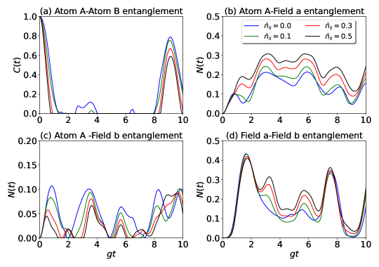
Figure 1. Entanglement dynamics of atom A-atom B, atom A-field a, atom A-field b, and field a-field b subsystems in DJCM with atomic states in the Bell state $\ket{\psi_{\textsubscript{AB}}}$ and field state in SCS. The other parameters are $\bar{n}_{c}=0.5$, $\theta=\frac{\pi}{4}$ and $\bar{n}_{s}=0.0,0.1,0.3,0.5$.

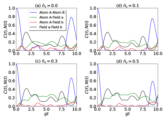
Figure 2. In this figure, entanglements for all the subsystems are plotted in a single plot for various $\bar{n}_{s}$ in DJCM with atomic states in the Bell state $\ket{\psi_{\textsubscript{AB}}}$ and field state in SCS.

In the previous section, we defined the states of radiation and atoms. We also investigated the evolution of the state of the atom-field system. In the present section, we explore the temporal evolution of entanglement for the radiation states with atoms in a Bell state.

3.1 For squeezed coherent states (SCS)

Figures 1 and 2 depict the entanglement dynamics between different subsystems of the atom-cavity system with a two-level atom in each cavity and each cavity field in a SCS. Here we have chosen $\bar{n}_{c}=0.5$ and $\bar{n}_{s}=0.0,0.1,0.3$ and $0.5$. In Fig. 1, entanglements between atom A-atom B, atom A-field a, atom A-field b and field a-field b are plotted for different values mentioned above of the mean squeezed photons $\bar{n}_{s}$. In Fig. 2, all these four entanglements have been plotted for a fixed $\bar{n}_{s}$. From Fig. 1(a), it is observed that the atom-atom entanglement falls very sharply with time for all $\bar{n}_{s}$ and ESD occurs in the dynamics. With increasing $\bar{n}_{s}$, the duration of these ESDs increases because the smaller peaks in the dynamics disappear. Here, in Fig. 1(a), it is seen that the largest ESD occurs for $\bar{n}_{s}=0.5$ (black curve in Fig. 1(a)). $C(t)$ revives again with different peak heights. The revival peak height decreases with increasing $\bar{n}_{s}$.

In Fig. 1(b) atom A-field a entanglement is plotted. It is seen that it starts from zero and increases with time. No ESD is observed for this atom A-field a entanglement. The amplitude of $N(t)$ increases with increasing $\bar{n}_{s}$. Squeezing in the field is transferring entanglement from atom A-atom B subsystem to atom A -field a and field a-field b subsystems. $N(t)$ for atom A-field b is represented in Fig. 1(c). Unlike the dynamics of $N(t)$ between atom A and field a, ESDs are observed in this case and the frequency of collapse and revival of $N(t)$ is larger compared to the case of the atom A-atom B entanglement dynamics. Fig. 1(d) shows the entanglement dynamics between fields a and b. The dynamics of $N(t)$ between field-field is almost opposite to the dynamics of $C(t)$ between the two atoms. $N(t)$ increases sharply and reaches a maximum value, when $C(t)$ for atom-atom entanglement shows ESD in the dynamics (see Fig. 1(a)). $N(t)$ comes down again and small peaks appear in the dynamics of $C(t)$ and it almost hits the zero line when $C(t)$ again becomes maximum. The complementary nature of atom-atom entanglement and filed-field entanglement is brought out in Figs. 1(a) and 1(d). It is also observed that $N(t)$ for field a-field b increases with increasing $\bar{n}_{s}$.

In Fig. 2, all four entanglements atom A-atom B, atom A-field a, atom A-field b and field a-field b are depicted for all the different values $\bar{n}_{s}$ mentioned before. From these plots, the dynamics of the entanglements can be compared with each other. It is observed how the evolution dynamics between two parties depend on the entanglement dynamics between other parties. Initially, only atom A-atom B entanglement is present and all other entanglements are zero. Then as $C(t)$ decreases with time, $N(t)$ for other bipartite systems increases. This exhibits the flow of entanglement between different subsystems.

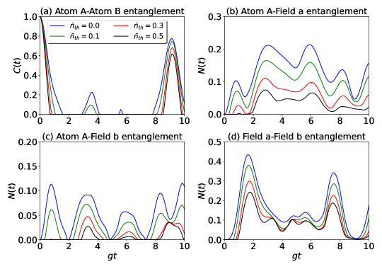
Figure 3. Entanglement dynamics of atom A-atom B, atom A-field a, atom A-field b, and field a-field b subsystems in DJCM with atomic states in the Bell state $\ket{\psi_{\textsubscript{AB}}}$ and field state in G-L states. Other parameters are $\bar{n}_{c}=0.5$, $\theta=\frac{\pi}{4}$ and $\bar{n}_{th}=0.0,0.1,0.3,0.5$.

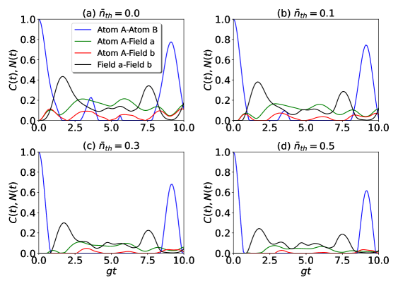
Figure 4. Here, entanglements for all the subsystems are plotted in a single plot for various $\bar{n}_{th}$ in DJCM with atomic states in the Bell state $\ket{\psi_{\textsubscript{AB}}}$ and field state in G-L states.

3.2 For Glauber-Lachs (G-L) states

The entanglement dynamics for G-L states are plotted in Figs. 3 and 4. For G-L states, we have chosen $\bar{n}_{c}=0.5$ and $\bar{n}_{th}=0.0,0.1,0.3$ and $0.5$. It is observed that the effects of $\bar{n}_{s}$ and $\bar{n}_{th}$ on atom A-atom B entanglement are quite similar (see Figs. 1(a) and 3(a)). A drastic difference in atom A-field a entanglement is observed. In the case of SCS, $N(t)$ increases with $\bar{n}_{s}$ (see Fig. 1(b)); but in the case of G-L states, $N(t)$ for atom A-field a decreases with increasing $\bar{n}_{th}$ (see Fig. 3(b)). It is quite contrasting.

For the field a-field b entanglement, in the case of SCS, the peak heights of $N(t)$ do not change; but, in between peak heights vary as $\bar{n}_{s}$ increases. However, in the case of G-L states, the peak heights of $N(t)$ for field-field entanglement fall very significantly with increasing $\bar{n}_{th}$. In the case of atom a-field b, the peak heights of $N(t)$ decrease for both $\bar{n}_{th}$ and $\bar{n}_{s}$ (see Fig. 1(c) and 3(c)); in the case of G-L states, $N(t)$ exhibits longer ESD’s for $\bar{n}_{th}=0.3$ and $0.5$ (red and black curves in Fig. 3(c)).

In Fig. 4, all four entanglements atom A-atom B, atom A-field a, atom A-field b and field a-field b for G-L states are depicted for all the different values $\bar{n}_{th}$ mentioned before.

4 Effects of spin-spin Ising interaction on entanglement dynamics for atoms in Bell state

In this section, the effects of spin-spin Ising interaction between the two atoms on entanglement dynamics of the atom-field system are studied. After including the Ising interaction term the total Hamiltonian becomes

$$\hat{H}_{\text{tot}}= \,\omega\hat{\sigma}_{z}^{\text{A}}+\omega\hat{\sigma}_{z}^{\text{B}}+g(\hat{a}^{\dagger}\sigma_{-}^{\text{A}}+\hat{a}\hat{\sigma}_{+}^{\text{A}})$$

$$+g(\hat{b}^{\dagger}\hat{\sigma}_{-}^{\text{B}}+\hat{b}\hat{\sigma}_{+}^{\text{B}})+\nu\hat{a}^{\dagger}\hat{a}+\nu\hat{b}^{\dagger}\hat{b}+J_{z}\hat{\sigma}_{\text{A}}^{z}\otimes\hat{\sigma}_{\text{B}}^{z},$$ (30)

where $\hat{\sigma}_{\text{A}}^{z}$ and $\hat{\sigma}_{\text{B}}^{z}$ are the spin operators for atom A and atom B respectively and $J_{z}$ is the coupling strength between the two atoms. $J_{z}$ has the unit of energy.

4.1 For squeezed coherent states

The effects of spin-spin Ising interaction between the atoms on the entanglement dynamics for SCS are shown in Fig. 5. To investigate the effects of Ising interaction for SCS, $\bar{n}_{c}=0.5$, $\bar{n}_{s}=0.1$ and $J_{z}=0.1,0.3,0.7,1.0$ are chosen. From Fig. 5(a), it is observed that the addition of $J_{z}=0.1$ decreases the length of ESDs in the dynamics of $C(t)$. More and more peaks of $C(t)$ appear in the dynamics with increasing amplitude for increasing $J_{z}$. But, for these values of $J_{z}$, the ESDs are not removed from the dynamics for $C(t)$. In Fig. 5(b), it is observed that $N(t)$ for atom A-field a does not change that much on adding the Ising interaction., Figs. 1(b) and 5(b) are mostly the same. In some places, the amplitude of $N(t)$ increases slightly due to the addition of $J_{z}$. Fig. 5(c) shows the effects of $J_{z}$ on $N(t)$ for atom A-field b. For $J_{z}=0.1$, it is seen that ESDs are almost removed from the dynamics. For $J_{z}=0.3,0.7,1.0$, it is observed that all the ESDs are removed from the dynamics and the amplitude of the highest peak of the dynamics increases with increasing $J_{z}$. The effect of the addition of $J_{z}$ on the field a-field b entanglement is interesting. It is observed that for $J_{z}=0.1$, all the ESDs are removed from the dynamics. However, it is noticeable that with increasing $J_{z}$, the amplitudes of the highest peaks of $N(t)$ fall down. This decrease in peak height of $N(t)$ is compensated by the increase in the peak of $C(t)$. Though $J_{z}$ is removing the ESDs from the dynamics of field-field entanglement, it is also reducing the amplitudes of $N(t)$. So, the spin-spin Ising interaction strengthens the atom A-atom B entanglement $C(t)$, but weakens the entanglement between two fields.

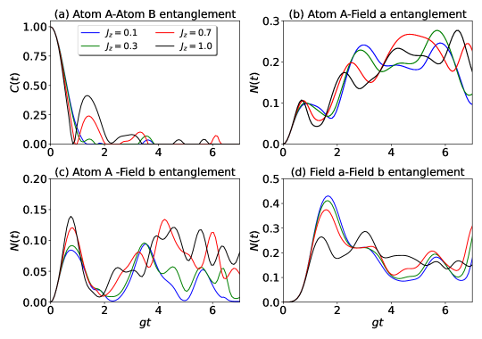
Figure 5. Effects of spin-spin Ising interaction entanglement dynamics of atom A-atom B, atom A-field a, atom A-field b, and field a-field b subsystems in DJCM for atomic states in the Bell state $\ket{\psi_{\textsubscript{AB}}}$ and field state in SCS. The other parameters are $\bar{n}_{c}=0.5,\bar{n}_{s}=0.1$, $\theta=\frac{\pi}{4}$ and $J_{z}=0.1,0.3,0.7,1.0$.

4.2 For Glauber-Lachs states

Figure 6 represents the plots of entanglement dynamics for G-L states with spin-spin Ising interaction present between the two atoms. For G-L states $\bar{n}_{c}=0.5$, $\bar{n}_{th}=0.1$ and $J_{z}=0.1,0.3,0.7,1.0$ are chosen. From Fig. 6(a), it is seen that for $J_{z}=0.1$, the duration of ESDs of $C(t)$ decreases and new peaks appear in the dynamics. As $J_{z}$ is increased more and more peaks appear making the duration of EDSs shorter. For $J_{z}=1.0$, there has been no ESD in the dynamics for a long while. If we compare Fig. 6(a) with Fig. 5(a), it can be observed that Ising interaction is more effective for G-L states than SCS to remove ESDs from the dynamics of $C(t)$. For atom A-field a dynamics in Fig. 6(b), the addition of $J_{z}$ decreases the amplitude of peaks of $N(t)$. In Fig. 6(c), for atom A-field b entanglement, it is seen that the Ising interaction reduces the length of ESDs for $J_{z}=0.1$. For $J_{z}=0.3,0.7$ and $1.0$, all the ESDs are removed from the dynamics. It is noticeable that for G-L states, Ising interaction is decreasing the atom A-field a entanglement, but increasing the atom A-field b entanglement. For the field a-field b entanglement, which is shown in Fig. 6(d), all the ESDs are removed from the dynamics corresponding to $J_{z}=0.1,0.3,0.7$ and $1.0$. Like SCS, for G-L states also, the initial highest peaks of $N(t)$ come down with the increasing value of $J_{z}$, however, for $J_{z}=0.3,0.7,1.0$, the amplitude of the entanglement $N(t)$ increases with time. So, the addition of spin-spin Ising interaction between the two atoms increases the entanglement in the atom-field system by removing the ESDs from the dynamics.

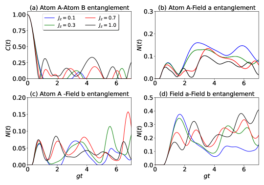
Figure 6. Effects of spin-spin Ising interaction on entanglement dynamics of atom A-atom B, atom A-field a, atom A-field b, and field a-field b subsystems in DJCM for atomic states in the Bell state $\ket{\psi_{\textsubscript{AB}}}$ and field state in G-L state. The other parameters are $\bar{n}_{c}=0.5,\bar{n}_{th}=0.1$, $\theta=\frac{\pi}{4}$ and $J_{z}=0.1,0.3,0.7,1.0$.

5 Effects of detuning on entanglement dynamics for atoms in Bell state

In this section, we study the effects of detuning present in the system. If detuning is present in the system, the effective Hamiltonian [10] of the system becomes

$$\hat{H}_{\text{eff}}=\Delta\hat{\sigma}_{-}\hat{\sigma}_{+}+g(\hat{a}^{\dagger}\sigma_{-}+\hat{a}\hat{\sigma}_{+}),$$ (31)

where $\Delta=\omega-\nu$ is the detuning of the atom-field system.

Figures $7$ and $8$ depict the entanglement dynamics for the SCS and G-L states respectively with the addition of detuning in the system. To observe the effects of $\Delta$ on the entanglement dynamics, we have taken $\bar{n}_{c}=0.5$, $\bar{n}_{s}=0.1$ and $\bar{n}_{th}=0.1$ for SCS and G-L states respectively and $\Delta$ is varied. In Fig. 7(a), $\bar{n}_{c}=0.5,\bar{n}_{s}=0.1,\Delta=2$ (black curve); here, for atom A-atom B entanglement, the addition of $\Delta$ reduces the ESD duration (see Figs. 1(a) and 7(a)). From Figs. 7(b), 7(c) and 7(d), it is evident that all the ESDs are removed from the dynamics of $N(t)$ for atom A-field a, atom A-field b and field a-field with the addition of $\Delta=2$, (black curves in the corresponding figures) in the system. Next, on increasing $\Delta$ to $5$, we see that the amplitude of $C(t)$ increases further and the number of ESD decreases (blue curve); however, for other entanglements the amplitude of $N(t)$ decreases significantly. For $\Delta=10$, more ESDs are removed from the dynamics of $C(t)$ with increasing amplitude and for other subsystems, the amplitudes of the entanglements reduce further. For field a-field b entanglement, $N(t)=0$ at the beginning of the dynamics and with time it revives, but with very low amplitudes in comparison with $N(t)$ for $\Delta=2$ and $5$.

In the case of G-L states, the effects of $\Delta$ on the entanglement dynamics are more prominent (see Fig. 8). Like SCS, for G-L states also, the addition of $\Delta=2$, decreases the duration of the ESDs for $C(t)$ and completely removes the ESDs for other subsystem entanglement; it also reduces the amplitude of $N(t)$. For $\Delta=5$, it is observed that $C(t)$ is completely free of ESDs; for all the other entanglements, ESDs appear again. With $\Delta=10$, $C(t)$ increases significantly; also, at the same time the duration of ESDs for atom A-field a, and atom A-field b increases further. For $\Delta=10$, field a-field b entanglement is almost totally lost.

From the above analysis, it comes out that detuning transfers entanglement to the atom-atom subsystem from atom-field and field-field subsystems. So, in the double J-C model, if we want to remove the ESDs from the dynamics of $C(t)$ and make the atom-atom subsystem more entangled, we need to add more detuning in the atom-field system.

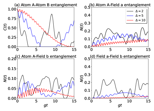
Figure 7. Effects of detuning on entanglement dynamics of atom A-atom B, atom A-field a, atom A-field b, and field a-field b subsystems with atomic states in the Bell state $\ket{\psi_{\textsubscript{AB}}}$ and field state in SCS for $\bar{n}_{c}=0.5,\bar{n}_{s}=0.1$, $\theta=\frac{\pi}{4}$ and $\Delta=2,5,10$.

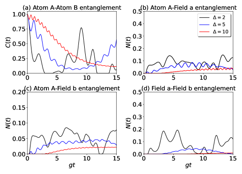
Figure 8. Effects of detuning on entanglement dynamics of atom A-atom B, atom A-field a, atom A-field b, and field a-field b subsystems with atomic states in the Bell state $\ket{\psi_{\textsubscript{AB}}}$ and field state in G-L states for $\bar{n}_{c}=0.5,\bar{n}_{th}=0.1$, $\theta=\frac{\pi}{4}$ and $\Delta=2,5,10$.

6 Effects of Kerr-nonlinearity on the entanglement dynamics for the two atoms in Bell state

After investigating the effects of Ising interaction and detuning, in this section, we study the effects of Kerr-nonlinearity on the entanglement of the atom-cavity system. After adding the Kerr-nonlinear term in the Hamiltonian, it becomes [41, 42, 43, 44, 45, 46, 47, 48, 49, 50]

$$\hat{H}_{\text{tot}}= \,\omega\hat{\sigma}_{z}^{\text{A}}+\omega\hat{\sigma}_{z}^{\text{B}}+g\left(\hat{a}^{\dagger}\hat{\sigma}_{-}^{\text{A}}+\hat{a}\,\hat{\sigma}_{+}^{\text{A}}\right)$$

$$+g\left(\hat{b}^{\dagger}\hat{\sigma}_{-}^{\text{B}}+\hat{b}\,\hat{\sigma}_{+}^{\text{B}}\right)+\,\nu\hat{a}^{\dagger}\hat{a}+\nu\hat{b}^{\dagger}\hat{b}+\chi\hat{a}^{\dagger 2}{\hat{a}}^{2}+\chi\hat{b}^{\dagger 2}\hat{b}^{2},$$ (32)

where $\chi=k\omega$ is the nonlinear coupling constant and $k$ is a non-negative number.

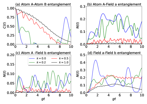
Figure 9. Effects of Kerr-nonlinearity on entanglement dynamics of atom A-atom B, atom A-field a, atom A-field b, and field a-field b subsystems for atomic states in Bell state $\ket{\psi_{\textsubscript{AB}}}$ and field state in SCS for $\bar{n}_{c}=0.5,\bar{n}_{s}=0.1$, $\theta=\frac{\pi}{4}$ and $k=0.0,0.2,0.5,1.0$.

Figures 9 and 10 show the effects of Kerr-nonlinearity on the entanglement dynamics of $\hat{H}_{\text{tot}}$ for SCS and G-L states respectively. Like detuning and spin-spin Ising interaction, Kerr-nonlinearity removes ESDs from the dynamics. From Fig. 9, it can be seen that for $k=0$, the atom A-Atom B entanglement has a long ESD (blue curve), which gets shortened for $k=0.2$ (represented by green colour), and for other subsystems, the associated ESDs are removed from the dynamics of $N(t)$. As we increase the value of $k$ to 0.5, the length of ESDs in $C(t)$ gets shortened further and the amplitudes of entanglement also increase prominently (red curve in Fig. 9). Also, the other associated entanglements atom A-field a and atom A-field b given by $N(t)$ drop abruptly, while for field a-field b, it drops initially but remains almost constant for a longer duration of time. For $k=1.0$, more ESDs are removed from the dynamics of $C(t)$ and its amplitude increases further (black curve); and, the amplitude of $N(t)$ for field-field entanglement falls drastically. Also, $N(t)$ for atom A-field a and atom A-field b becomes very close to zero; $N(t)$ even touches zero at some places.

In the case of G-L states (see Fig. 10), for $k=0.2$, the ESDs are removed from the dynamics of $C(t)$ and from $N(t)$ of atom A-field b and field a-field b. The amplitudes of atom A-atom B entanglement and atom A-field b entanglement increase significantly; but, for field a-field b entanglement the peak of $N(t)$ decreases remarkably. However, for atom A-field a entanglement, $N(t)$ vanishes at certain instants of time. For $k=0.5$, $C(t)$ attains values much higher in comparison with those corresponding to lower $k$ values; also, the oscillations are of smaller amplitudes. For $N(t)$ of other subsystems, ESDs become more prominent. As we increase $k$ to $1.0$, it is observed that $C(t)$ tends towards the maximum value of $C(t)=1$ and $N(t)$ for all the other entanglements are almost zero i.e., all entanglements are transferred to the atom-atom system.

So, like detuning, Kerr-nonlinearity also transfers the entanglement from other subsystems to the atom-atom subsystem. Figures 13 and 15 show how entanglement gets transferred from other subsystems to the atom-atom subsystem for SCS and G-L states respectively.

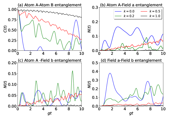
Figure 10. Effects of Kerr-nonlinearity on entanglement dynamics of atom A-atom B, atom A-field a, atom A-field b, and field a-field b subsystems for atomic states in Bell state $\ket{\psi_{\textsubscript{AB}}}$ and field state in G-L states for $\bar{n}_{c}=0.5,\bar{n}_{th}=0.1$, $\theta=\frac{\pi}{4}$ and $k=0.0,0.2,0.5,1.0$.

7 Entanglement dynamics for SCS and G-L states of radiation inside the cavities with the atoms in Werner state

In this section, the entanglement dynamics for SCS and G-L states with atoms in Werner state (mixed state) are investigated.

7.1 For SCS

To study the dynamics for SCS with atoms in a Werner state, $\bar{n}_{c}=0.5$, and $\bar{n}_{s}=0.0,0.1,0.3,0.5$ are taken. The entanglement dynamics for SCS with the two-level atoms in a Werner state are plotted in Figs. 11 and 12. For the Werner state, mixing parameter $\lambda=0.75$ is taken. Like the atoms being in a Bell state, for the Werner state, similar dynamics of $C(t)$ and $N(t)$ are also observed (see Figs. 1 and 11). From Fig. 11(a), here also, we see that the length of ESD in atom A-atom B entanglement increases with increasing $\bar{n}_{s}$. The atom A-field a and field a-field b entanglement increase with increasing $\bar{n}_{s}$ which is evident from Figs. 11(b) and 11(d), but atom A-field b entanglement (Fig. 11(c)) decreases with increasing $\bar{n}_{s}$.

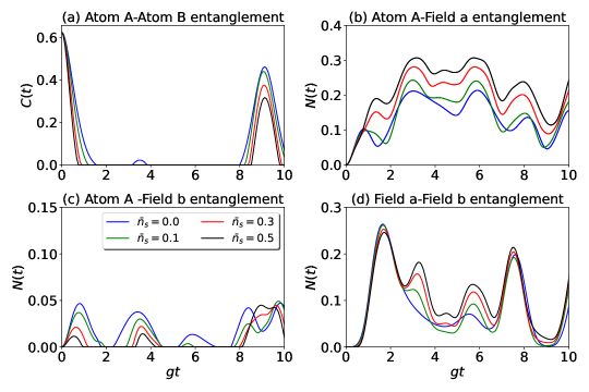
Figure 11. Entanglement dynamics of atom A-atom B, atom A-field a, atom A-field b, and field a-field b subsystems in DJCM with atomic states in Werner state and field state in SCS. The other parameters $\bar{n}_{c}=0.5$, $\lambda=0.75$ and $\bar{n}_{s}=0.0,0.1,0.3,0.5$.

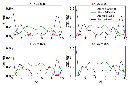
Figure 12. In this figure, entanglements for all the subsystems are plotted in a single plot for various $\bar{n}_{s}$ in DJCM with atomic states in Werner state and field state in SCS.

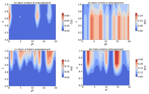
Figure 13. Contour plots of entanglement dynamics $C(t)$ and $N(t)$ $vs$ $gt$ and $\lambda$ of different subsystems for SCS with atoms in Werner state. Other parameters in these plots are $\bar{n}_{c}=0.5,\bar{n}_{s}=0.1$.

7.2 For G-L state

For G-L states, with atoms in Werner state, $\bar{n}_{c}=0.5$, $\lambda=0.75$ and $\bar{n}_{th}=0.0,0.1,0.3,0.5$ are taken. Figs. 14 and 15 show the entanglement dynamics for the G-L state with the atoms in a Werner state. If we compare Figs. 3 and 14, it is seen that for G-L states, $C(t)$ and $N(t)$ show almost similar dynamics for atoms in the Bell state and in the Werner state. In Fig. 3(a), there are two smaller peaks present in the dynamics for $\bar{n}_{th}=0.1$, however here only is present; which makes the length of ESD a little larger. So, we observe that $C(t)$ and $N(t)$ do not show any noticeable difference in their dynamics if the atoms are in a Bell state or in a Werner state when no other interactions or detuning are present in the system.

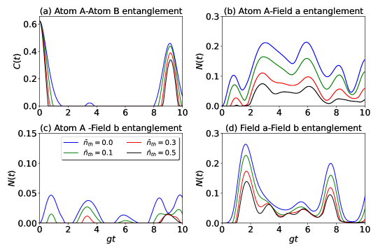
Figure 14. Entanglement dynamics of atom A-atom B, atom A-field a, atom A-field b, and field a-field b subsystems in DJCM with atomic states in Werner state and field state in G-L states. The other parameters $\bar{n}_{c}=0.5$, $\lambda=0.75$ and $\bar{n}_{th}=0.0,0.1,0.3,0.5$.

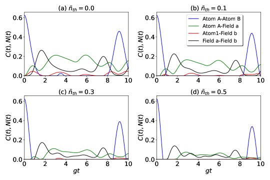
Figure 15. In this figure, entanglements for all the subsystems are plotted in a single plot for various in DJCM with atomic states in Werner state and field state in G-L states.

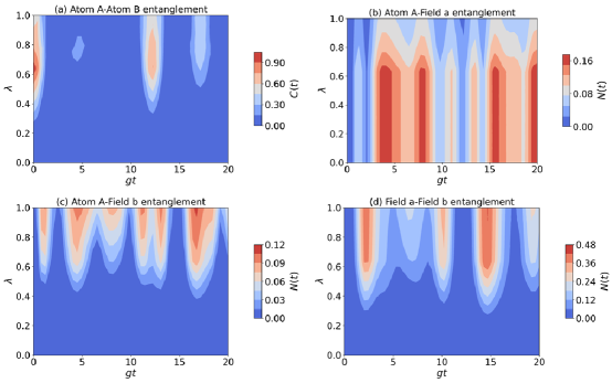
Figure 16. Contour plots of entanglement dynamics $C(t)$ and $N(t)$ $vs$ $gt$ and $\lambda$ for G-L states with the atoms in Werner state. Other parameters in the plot are $\bar{n}_{c}=0.5,\bar{n}_{th}=0.1$.

The contour plots in Figs. 13 and 16 show how $C(t)$ and $N(t)$ behave with varying $\lambda$ for SCS and G-L states respectively. For these plots we have fixed $\bar{n}_{c}=0.5$, $\bar{n}_{s}=0.1$ and $\bar{n}_{th}=0.1$ for SCS and G-L states respectively. From these figures, we observe that for $\lambda<0.3$, the atomic state is a separable state and there is no entanglement present in the system except atom A-field a entanglement. This entanglement is present because of the single Jaynes-Cummings interaction inside each cavity. It is also observed that atom A-field b and field a-field b entanglements increase with increasing $\lambda$. On the other hand $C(t)$ of atom A-atom B and $N(t)$ of atom A-field a entanglement reach maximum for certain values of $\lambda$, after that $C(t)$ and $N(t)$ decrease.

8 Effects of Ising interaction for SCS and G-L states with atoms in Werner state

In this section, the effects of spin-spin Ising interaction on entanglement are observed for the atoms in the Werner state.

8.1 For $\lambda=0.75$

The effects of Ising interaction with atoms in the Werner state for SCS are represented in Fig. 17. Like for the atoms being in Bell state, for Werner state also, the length of ESDs in the dynamics of $C(t)$ decreases with increasing $\bar{n}_{s}$. From Fig. 17(a), we observe that $J_{z}$ tries to remove the ESDs by reducing the death time of the dynamics. The amplitudes of entanglement increase and death time decreases with the increasing value of $J_{z}$. But, in the case of atoms in the Bell state, $J_{z}$ removes the ESDs more efficiently (see Fig. 5) as compared to the case of the atoms in the Werner state. For atom A-field a subsystem, it is noticed that for the Werner state also, the addition of Ising interaction decreases the amplitude of entanglement and tries to create ESDs in the dynamics. For both atom A-field b and field a-field b subsystems, the addition of $J_{z}$ removes all ESDs from the dynamics of $N(t)$; also $N(t)$ increases with time when $J_{z}$ increases.

The effects of Ising interaction on the entanglement dynamics for G-L states are shown in Fig. 18. Similar kinds of results are observed in entanglement dynamics for G-L states. The addition of $J_{z}$ tries to remove the ESDs from the dynamics of $C(t)$ and $N(t)$ for atom A-field b and field a-field b. But, for the atom A-field a subsystem, entanglement decreases with increasing $J_{z}$ and tends to ESD.

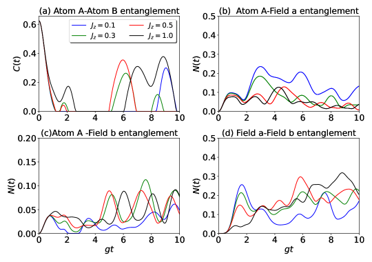
Figure 17. Effects of spin-spin Ising interaction on entanglement dynamics of atom A-atom B, atom A-field a, atom A-field b, and field a-field b subsystems in DJCM with atomic states in Werner state and field state in SCS. Other parameters are $\bar{n}_{c}=0.5,\bar{n}_{s}=0.1$, $\lambda=0.75$ and $J_{z}=0.1,0.3,0.7,1.0$.

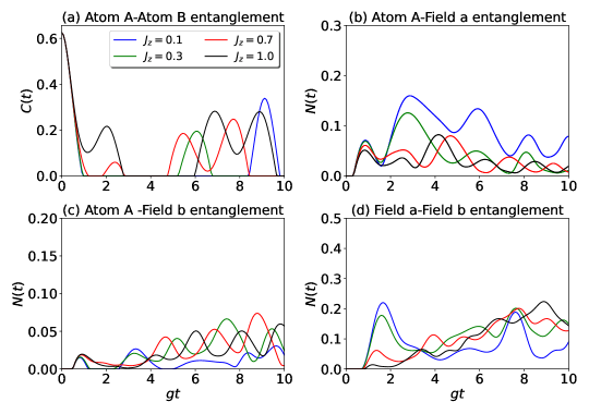
Figure 18. Effects of spin-spin Ising interaction on entanglement dynamics of atom A-atom B, atom A-field a, atom A-field b, and field a-field b subsystems in DJCM with atomic states in Werner state and field state in G-L states. Other parameters are $\bar{n}_{c}=0.5,\bar{n}_{th}=0.1$, $\lambda=0.75$ and $J_{z}=0.1,0.3,0.7,1.0$.

8.2 For $\lambda=0.25$

Fig. 19 shows the entanglement dynamics for SCS for $\lambda=0.25$ without any spin-spin Ising interaction between the atoms. For $\lambda=0.25$, Werner state is a separable state; so there is no initial entanglement present in the system. The plots show the expected dynamics for $C(t)$ and $N(t)$. In this initial atomic state, none of atom A-atom B, atom A-field b and field a-field b entanglement is present in the system; only atom A-field a entanglement is observed which is just the normal Jaynes-Cummings interaction between a single two-level atom and a radiation field. Similar dynamics are observed for G-L states also which we have not included here.

If Ising interaction is present in the system, different phenomena are noticed. It is observed that all the subsystems atom A-atom B, atom A-field a, atom A-field b and field a-field b get entangled. Fig. 20 and 21 show the contour plots of $C(t)$ and $N(t)$ for SCS and G-L states respectively for $\lambda=0.25$ while $J_{z}$ $\in[0,1]$. From Fig. 20(a), we see that for a wide range of $J_{z}$, $C(t)$ shows a positive value of entanglement, however, in the case of G-L states in Fig. 21(a), $C(t)$ shows positive values for a very narrow range of values of $J_{z}$. For both states of radiation, $N(t)$ for atom A-field a and field a-field b subsystems show prominent values for almost all values of $J_{z}$ while $N(t)$ for atom A-field b subsystems are quite small. From these plots, it is also evident that atom A-field b entanglement increases with increasing value of $J_{z}$ and atom A-field a entanglement decreases. So, it can be concluded that $J_{z}$ transfers the entanglement from atom A-field a subsystem to other subsystems.

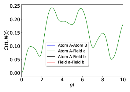
Figure 19 . Entanglement dynamics of atom A-atom B, atom A-field a, atom A-field b, and field a-field b subsystems in DJCM for field state SCS and atomic state in Werner state with $\lambda=0.25$ and without any Ising interaction between the two atoms.

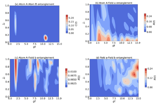
Figure 20. Contour plots of entanglement dynamics of atom A-atom B, atom A-field a, atom A-field b, and field a-field b subsystems with spin-spin Ising interaction in DJCM for SCS and atomic state in Werner ($\lambda=0.25$). Here, other parameters are $\bar{n}_{c}=0.5$ and $\bar{n}_{s}=0.1$.

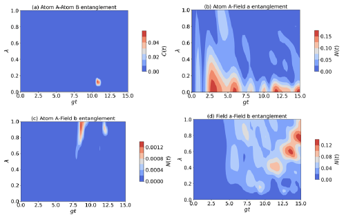
Figure 21. Contour plots of entanglement dynamics of atom A-atom B, atom A-field a, atom A-field b, and field a-field b subsystems with spin-spin Ising interaction in DJCM for G-L states and atomic state in Werner state ($\lambda=0.25$). Here, other parameters are $\bar{n}_{c}=0.5$ and $\bar{n}_{th}=0.1$.

9 Effects of detuning for SCS and G-L states with atoms in Werner state

In this section, we study the effects of detuning on the entanglement dynamics for SCS and G-L states with the atoms in a Werner state. Figs. 22 and 23 show the effects of detuning on $C(t)$ and $N(t)$ for SCS and G-L with atoms in a Werner state respectively. Like the atoms in a Bell state, for the Werner state also, adding detuning in the system tries to remove ESDs from the dynamics of $C(t)$. In Fig. 22(a), it is observed that the addition of $\Delta=2$ (black curve) reduces the duration of ESD (compare Figs. 14(a) and 22(a)). As we increase $\Delta$ to 5, the amplitude of $C(t)$ increases further and the number of ESDs decreases (blue curve). With $\Delta=10$, the amplitude increases more and the length of ESDs also decreases. $C(t)$.

In Fig. 22(b), we observe a similar kind of behaviour as observed in Fig. 7(b). $N(t)$ for atom A-field a decreases with the increasing $\Delta$ in a similar pattern as was in the case of atoms in a Bell state. For atom A-field b also, similar kinds of dynamics of $N(t)$ are observed. In the case of field a-field b entanglement, the addition of $\Delta=2$ increases ESDs in $N(t)$ (see Fig. 22(d)) and ESDs appear at the beginning of dynamics. More ESDs appear and the amplitudes of $N(t)$ decrease for $\Delta=5$. If detuning is increased further to $\Delta=10$, the field a-field b entanglement admits a total ESD (see Fig. 22(d)). All these dynamics suggest that the death or decrease in the entanglement of atom-field and field-field entanglements contribute to the increment in the entanglement of atom a-atom b. So, with the atoms in a Werner state also, $\Delta$ transfers the entanglement from other subsystems to the atom-atom subsystem.

In the case of G-L states (Fig. 23), $\Delta$ affects the dynamics of $C(t)$ and $N(t)$ almost in a similar way as it does for SCS, however $N(t)$ loses its amplitude faster. For $\Delta=5$, $N(t)$ becomes zero and total death in the entanglement is observed for atom A-field b and field a-field b subsystems. When $\Delta=10$, from Fig. 23(a) it is observed that ESDs are not completely removed from the dynamics of $C(t)$ in the case of atoms in the Werner state; though the amplitude of $C(t)$ increases significantly. If we compare Figs. 23(a) and 8(a), it can be concluded that $\Delta$ is more efficient in removing ESDs from the dynamics with atoms in a Bell state.

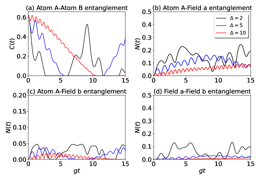
Figure 22. Effects of detuning on entanglement dynamics of atom A-atom B, atom A-field a, atom A-field b, and field a-field b subsystems with atomic states in Werner state and field state in SCS for $\bar{n}_{c}=0.5,\bar{n}_{s}=0.1$, $\lambda=0.75$ and $\Delta=2,5,10$.

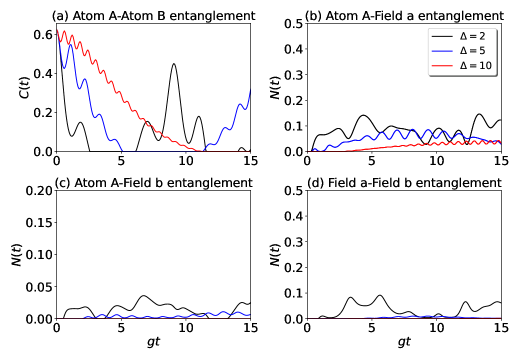
Figure 23. Effects of detuning on entanglement dynamics of atom A-atom B, atom A-field a, atom A-field b, and field a-field b subsystems with atomic states in Werner state and field state in SCS for $\bar{n}_{c}=0.5,\bar{n}_{th}=0.1$, $\lambda=0.75$ and $\Delta=2,5,10$.

10 Effects of Kerr-nonlinearity on the entanglement dynamics of atom-cavity system with atoms in Werner state

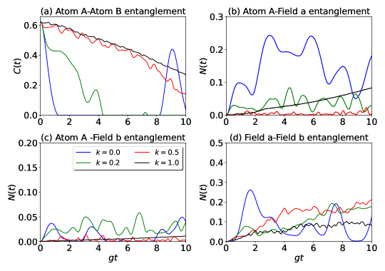
Figure 24. Effects of Kerr-nonlinearity on entanglement dynamics of atom A-atom B, atom A-field a, atom A-field b, and field a-field b subsystems with atomic states in Werner state and field in SCS for $\bar{n}_{c}=0.5,\bar{n}_{s}=0.1$, $\lambda=0.75$ and $k=0.0,0.2,0.5,1.0$.

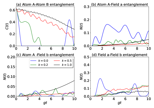
Figure 25. Effects of Kerr-nonlinearity on entanglement dynamics of atom A-atom B, atom A-field a, atom A-field b, and field a-field b subsystems with atomic states in Werner state and field in G-L states for $\bar{n}_{c}=0.5,\bar{n}_{s}=0.1$, $\theta=\frac{\pi}{4}$ and $k=0.0,0.2,0.5,1.0$.

The effects of Kerr-nonlinearity on the entanglement dynamics for SCS and G-L states with atoms in a Werner state are plotted in Figs. 24 and 25 respectively. As before, $\bar{n}_{c}=0.5,\bar{n}_{s}=0.1$, $\bar{n}_{th}=0.1$, $k=0.0,0.2,0.5,1.0$ and the mixing parameter $\lambda=0.75$. From Fig. 24(a), it is evident that the addition of non-linearity removes the ESDs from the dynamics of $C(t)$ very effectively. In the case of atom A-field a, $N(t)$ shows strange behaviour to the addition of $k$ in the system. At first, with the increasing value of $k$, $N(t)$ decreases rapidly and an almost ESD is observed (see red curve in Fig. 24(b)). However, when $k$ is increased to 1, we see that $N(t)$ rises up (see the black curve in Fig. 24(b). Similar behaviour is observed for atom A-field b subsystem, which is depicted in Fig. 24(c). Such an unusual behaviour is not present in the case of atoms in the Bell state.

It is evident from Fig. 25 that in the case of G-L states, the effects of Kerr-nonlinearity are almost similar to those for SCS. The only noticeable difference is that $N(t)$ for atom A-field b increases more rapidly for $k=1.0$ in the case of G-L states (Fig. 25(c)).

11 Conclusion

Effects of thermal photons $\bar{n}_{th}$ and squeezed photons $\bar{n}_{s}$ in coherent background on entanglement dynamics with atoms in a Bell state and Werner state have been studied. For both Bell and Werner states, it is observed that the effects of $\bar{n}_{th}$ and $\bar{n}_{s}$ on atom A-atom B entanglement are almost similar. But, for other subsystems, it is quite different. $N(t)$ for atom A-field a and field a-field b subsystems decreases with increasing $\bar{n}_{th}$, however for SCS, $N(t)$ increases with increasing $\bar{n}_{s}$.

The effects of Ising interaction on entanglement dynamics for SCS and G-L states are almost similar to the atoms in the Bell state(pure state) or in the Werner state (mixed state). For both SCS and G-L states, with atoms in a pure or mixed state, the addition of spin-spin Ising interaction in the system tries to remove the ESDs from the dynamics of $C(t)$ and $N(t)$ for atom A-atom B, atom A-field b and field a-field b subsystems. However, for atom A-field a subsystem, in the case of SCS, the addition of $J_{z}$ increases the value of $N(t)$ but for G-L states $N(t)$ is decreased significantly. $J_{z}$ creates entanglement in the atom-field system. With atoms in a Werner state, for $\lambda=0.25$, it is a separable state. So, the initial atomic state is unentangled. So, the system is like two separated atoms in two different cavities. The time evolution of entanglement of the atom-cavity system is just two independent J-C interaction type dynamics. However, if spin-spin Ising interaction is introduced in the system, entanglement is observed between the subsystems of the whole atom-field system.

Detuning also affects entanglements for both the states of radiation field SCS and G-L states with the atoms in pure (Bell) and mixed (Werner) states in a similar way. All the ESDs are removed from the dynamics of the atom-atom subsystem with increasing $\Delta$. However, ESDs are observed for other subsystems. It is like, $\Delta$ is transferring all the entanglements to the atom-atom subsystem from the other subsystems. Like detuning, Kerr-nonlinearity also removes ESDs from the dynamics of $C(t)$ and $N(t)$. With an increasing value of $k$, $C(t)$ increases but $N(t)$ decreases creating almost sudden deaths in the entanglement of other subsystems. So, the addition of Kerr-nonlinearity also transfers entanglement to the atom-atom subsystem from the other three subsystems.

12 Acknowledgements

The authors are benefited by the discussions with Professor Arul Lakshminarayan. One of the authors KM is grateful to DST for the financial support from the project PH2021039DSTX008128.

References

- [1] Jaynes, E. T. & Cummings, F. W. Comparison of quantum and semiclassical radiation theories with application to the beam maser. Proceedings of the IEEE 51, 89–109 (1963). URL https://doi.org/10.1109/PROC.1963.1664.
- [2] Chong, S. Y. & Shen, J. Q. Quantum collapse-revival effect in a supersymmetric jaynes–cummings model and its possible application in supersymmetric qubits. Physica Scripta 95, 055104 (2020). URL https://dx.doi.org/10.1088/1402-4896/ab5c6e.
- [3] Nayak, N., Bullough, R., Thompson, B. & Agarwal, G. Quantum collapse and revival of rydberg atoms in cavities of arbitrary q at finite temperature. IEEE journal of quantum electronics 24, 1331–1337 (1988). URL https://ieeexplore.ieee.org/stamp/stamp.jsp?tp=&arnumber=971.
- [4] Gea-Banacloche, J. Collapse and revival of the state vector in the jaynes-cummings model: An example of state preparation by a quantum apparatus. Physical review letters 65, 3385 (1990). URL https://link.aps.org/doi/10.1103/PhysRevLett.65.3385.
- [5] Karatsuba, A. A. & Karatsuba, E. A. A resummation formula for collapse and revival in the jaynes–cummings model. Journal of Physics A: Mathematical and Theoretical 42, 195304 (2009). URL https://dx.doi.org/10.1088/1751-8113/42/19/195304.
- [6] Cirac, J., Blatt, R., Parkins, A. & Zoller, P. Quantum collapse and revival in the motion of a single trapped ion. Physical Review A 49, 1202 (1994). URL https://link.aps.org/doi/10.1103/PhysRevA.49.1202.
- [7] Jakubczyk, P., Majchrowski, K. & Tralle, I. Quantum entanglement in double quantum systems and jaynes-cummings model. Nanoscale research letters 12, 1–9 (2017). URL https://doi.org/10.1186/s11671-017-1985-0.
- [8] Vogel, W. & Welsch, D.-G. k-photon jaynes-cummings model with coherent atomic preparation: Squeezing and coherence. Physical Review A 40, 7113 (1989). URL https://link.aps.org/doi/10.1103/PhysRevA.40.7113.
- [9] Yonac, M., Yu, T. & Eberly, J. Sudden death of entanglement of two jaynes-cummings atoms. Journal of Physics B Atomic Molecular and Optical Physics 39 (2006). URL https://www.researchgate.net/publication/2197779.
- [10] Li, Z.-j., Zhang, J., Hu, P. & Han, Z.-w. Entanglement dynamics of two atoms in the squeezed vacuum and the coherent fields. International Journal of Theoretical Physics 59, 730–742 (2020). URL https://doi.org/10.1007/s10773-019-04359-2.
- [11] Qin, X. & Mao-Fa, F. Entanglement dynamics of the double intensity-dependent coupling jaynes-cummings models. International Journal of Theoretical Physics 51, 778–786 (2012). URL https://doi.org/10.1007/s10773-011-0957-x.
- [12] Pandit, M., Das, S., Roy, S. S., Dhar, H. S. & Sen, U. Effects of cavity–cavity interaction on the entanglement dynamics of a generalized double jaynes–cummings model. Journal of Physics B: Atomic, Molecular and Optical Physics 51, 045501 (2018). URL https://doi.org/10.1088/1361-6455/aaa2cf.
- [13] Ghoshal, A., Das, S., Sen(De), A. & Sen, U. Population inversion and entanglement in single and double glassy jaynes-cummings models. Phys. Rev. A 101, 053805 (2020). URL https://link.aps.org/doi/10.1103/PhysRevA.101.053805.
- [14] Obada, A.-S. F., Khalil, E., Ahmed, M. & Elmalky, M. International Journal of Theoretical Physics 57, 2787–2801 (2018). URL https://doi.org/10.1007/s10773-018-3799-y.
- [15] Chaturvedi, S. & Srinivasan, V. Photon-number distributions for fields with gaussian wigner functions. Phys. Rev. A 40, 6095–6098 (1989). URL https://link.aps.org/doi/10.1103/PhysRevA.40.6095.
- [16] Janszky, J. & Yushin, Y. Many-photon processes with the participation of squeezed light. Phys. Rev. A 36, 1288–1292 (1987). URL https://link.aps.org/doi/10.1103/PhysRevA.36.1288.
- [17] Marian, P. & Marian, T. A. Squeezed states with thermal noise. i. photon-number statistics. Phys. Rev. A 47, 4474–4486 (1993). URL https://link.aps.org/doi/10.1103/PhysRevA.47.4474.
- [18] Marian, P. & Marian, T. A. Squeezed states with thermal noise. ii. damping and photon counting. Phys. Rev. A 47, 4487–4495 (1993). URL https://link.aps.org/doi/10.1103/PhysRevA.47.4487.
- [19] Vourdas, A. Superposition of squeezed coherent states with thermal light. Phys. Rev. A 34, 3466–3469 (1986). URL https://link.aps.org/doi/10.1103/PhysRevA.34.3466.
- [20] Yi-min, L., Hui-rong, X., Zu-geng, W. & Zai-xin, X. Squeezed coherent thermal state and its photon number distribution. Acta Physica Sinica (Overseas Edition) 6, 681 (1997). URL https://doi.org/10.1088/1004-423x/6/9/006.
- [21] Ezawa, H., Mann, A., Nakamura, K. & Revzen, M. Characterization of thermal coherent and thermal squeezed states. Annals of Physics 209, 216–230 (1991). URL https://www.sciencedirect.com/science/article/pii/000349169190360K.
- [22] Kim, M. S., de Oliveira, F. A. M. & Knight, P. L. Properties of squeezed number states and squeezed thermal states. Phys. Rev. A 40, 2494–2503 (1989). URL https://link.aps.org/doi/10.1103/PhysRevA.40.2494.
- [23] Yamamoto, Y. & Haus, H. A. Preparation, measurement and information capacity of optical quantum states. Rev. Mod. Phys. 58, 1001–1020 (1986). URL https://link.aps.org/doi/10.1103/RevModPhys.58.1001.
- [24] Kitagawa, M. & Ueda, M. Squeezed spin states. Phys. Rev. A 47, 5138–5143 (1993). URL https://link.aps.org/doi/10.1103/PhysRevA.47.5138.
- [25] Ralph, T. C. Continuous variable quantum cryptography. Phys. Rev. A 61, 010303 (1999). URL https://link.aps.org/doi/10.1103/PhysRevA.61.010303.
- [26] Hillery, M. Quantum cryptography with squeezed states. Phys. Rev. A 61, 022309 (2000). URL https://link.aps.org/doi/10.1103/PhysRevA.61.022309.
- [27] Braunstein, S. L. & Kimble, H. J. Teleportation of continuous quantum variables. Phys. Rev. Lett. 80, 869–872 (1998). URL https://link.aps.org/doi/10.1103/PhysRevLett.80.869.
- [28] Milburn, G. J. & Braunstein, S. L. Quantum teleportation with squeezed vacuum states. Phys. Rev. A 60, 937–942 (1999). URL https://link.aps.org/doi/10.1103/PhysRevA.60.937.
- [29] Satyanarayana, M. V., Vijayakumar, M. & Alsing, P. Glauber-lachs version of the jaynes-cummings interaction of a two-level atom. Phys. Rev. A 45, 5301–5304 (1992). URL https://link.aps.org/doi/10.1103/PhysRevA.45.5301.
- [30] Sivakumar, S. Effect of thermal noise on atom-field interaction: Glauber-lachs versus mixing. The European Physical Journal D 66, 1–7 (2012). URL https://doi.org/10.1140/epjd/e2012-30399-2.
- [31] Mandal, K. & Satyanarayana, M. Atomic inversion and entanglement dynamics for squeezed coherent thermal states in the jaynes-cummings model. International Journal of Theoretical Physics 62, 1–19 (2023). URL https://doi.org/10.1007/s10773-023-05389-7.
- [32] Elben, A. et al. Mixed-state entanglement from local randomized measurements. Phys. Rev. Lett. 125, 200501 (2020). URL https://link.aps.org/doi/10.1103/PhysRevLett.125.200501.
- [33] Schmid, C. et al. Experimental direct observation of mixed state entanglement. Phys. Rev. Lett. 101, 260505 (2008). URL https://link.aps.org/doi/10.1103/PhysRevLett.101.260505.
- [34] Murciano, S., Vitale, V., Dalmonte, M. & Calabrese, P. Negativity hamiltonian: An operator characterization of mixed-state entanglement. Phys. Rev. Lett. 128, 140502 (2022). URL https://link.aps.org/doi/10.1103/PhysRevLett.128.140502.
- [35] Yuen, H. P. Two-photon coherent states of the radiation field. Physical Review A 13, 2226 (1976). URL https://link.aps.org/doi/10.1103/PhysRevA.13.2226.
- [36] Subeesh, T., Sudhir, V., Ahmed, A. B. M. & Satyanarayana, M. V. Effect of squeezing on the atomic and the entanglement dynamics in the jaynes-cummings model. Nonlinear Optics and Quantum Optics 44, 1–14 (2012). URL https://arxiv.org/abs/1203.4792.
- [37] Filipowicz, P. Quantum revivals in the jaynes-cummings model. Journal of Physics A: Mathematical and General 19, 3785 (1986). URL https://dx.doi.org/10.1088/0305-4470/19/18/024.
- [38] Puri, R. R. & Agarwal, G. S. Finite-q cavity electrodynamics: Dynamical and statistical aspects. Phys. Rev. A 35, 3433–3449 (1987). URL https://link.aps.org/doi/10.1103/PhysRevA.35.3433.
- [39] Wootters, W. K. Entanglement of formation and concurrence. Quantum Inf. Comput. 1, 27–44 (2001).
- [40] Wei, T.-C. et al. Maximal entanglement versus entropy for mixed quantum states. Physical Review A 67, 022110 (2003). URL https://link.aps.org/doi/10.1103/PhysRevA.67.022110.
- [41] Góra, P. & Jedrzejek, C. Nonlinear jaynes-cummings model. Phys. Rev. A 45, 6816–6828 (1992). URL https://link.aps.org/doi/10.1103/PhysRevA.45.6816.
- [42] Joshi, A. & Puri, R. R. Dynamical evolution of the two-photon jaynes-cummings model in a kerr-like medium. Phys. Rev. A 45, 5056–5060 (1992). URL https://link.aps.org/doi/10.1103/PhysRevA.45.5056.
- [43] Werner, M. J. & Risken, H. Quasiprobability distributions for the cavity-damped jaynes-cummings model with an additional kerr medium. Phys. Rev. A 44, 4623–4632 (1991). URL https://link.aps.org/doi/10.1103/PhysRevA.44.4623.
- [44] Ahmed, A. & Sivakumar, S. Dynamics of entanglement in a two-mode nonlinear jaynes-cummings mode. arXiv preprint arXiv:0907.2992 (2009). URL https://doi.org/10.48550/arXiv.0907.2992.
- [45] Sivakumar, S. Nonlinear jaynes–cummings model of atom–field interaction. International Journal of Theoretical Physics 43, 2405–2421 (2004). URL https://doi.org/10.1007/s10773-004-7707-2.
- [46] Mo, C., Xu, K. & Zhang, G.-F. The entanglement and second-order coherence function in a two-atom nonlinear jaynes-cummings model. Physica Scripta 97, 035101 (2022). URL https://dx.doi.org/10.1088/1402-4896/ac4cfe.
- [47] Xiong, W., Tian, M., Zhang, G.-Q. & You, J. Q. Strong long-range spin-spin coupling via a kerr magnon interface. Phys. Rev. B 105, 245310 (2022). URL https://link.aps.org/doi/10.1103/PhysRevB.105.245310.
- [48] Baghshahi, H., Tavassoly, M. & Faghihi, M. Entanglement analysis of a two-atom nonlinear jaynes–cummings model with nondegenerate two-photon transition, kerr nonlinearity, and two-mode stark shift. Laser Physics 24, 125203 (2014). URL https://dx.doi.org/10.1088/1054-660X/24/12/125203.
- [49] Zheng, L. & Zhang, G.-F. Intrinsic decoherence in jaynes-cummings model with heisenberg exchange interaction. The European Physical Journal D 71, 1–4 (2017). URL https://doi.org/10.1140/epjd/e2017-80408-y.
- [50] Xiong, W., Jin, D.-Y., Qiu, Y., Lam, C.-H. & You, J. Q. Cross-kerr effect on an optomechanical system. Phys. Rev. A 93, 023844 (2016). URL https://link.aps.org/doi/10.1103/PhysRevA.93.023844.