Competitive Advantage Attacks to Decentralized Federated Learning
Abstract
Decentralized federated learning (DFL) enables clients (e.g., hospitals and banks) to jointly train machine learning models without a central orchestration server. In each global training round, each client trains a local model on its own training data and then they exchange local models for aggregation. In this work, we propose SelfishAttack, a new family of attacks to DFL. In SelfishAttack, a set of selfish clients aim to achieve competitive advantages over the remaining non-selfish ones, i.e., the final learnt local models of the selfish clients are more accurate than those of the non-selfish ones. Towards this goal, the selfish clients send carefully crafted local models to each remaining non-selfish one in each global training round. We formulate finding such local models as an optimization problem and propose methods to solve it when DFL uses different aggregation rules. Theoretically, we show that our methods find the optimal solutions to the optimization problem. Empirically, we show that SelfishAttack successfully increases the accuracy gap (i.e., competitive advantage) between the final learnt local models of selfish clients and those of non-selfish ones. Moreover, SelfishAttack achieves larger accuracy gaps than poisoning attacks when extended to increase competitive advantages.
1 Introduction
In decentralized federated learning (DFL) [8, 12, 22, 9, 23, 21, 24], multiple clients (e.g., hospitals or banks) jointly train machine learning models without a central orchestration server. Specifically, each client maintains a local model. In each global training round, each client trains its local model (called pre-aggregation local model) using its local training data, shares a model (called shared model) with other clients, and aggregates the shared models from all clients as a new local model (called post-aggregation local model) according to an aggregation rule. For instance, when the aggregation rule is FedAvg [18], a client’s post-aggregation local model is the mean of the shared models from all clients. In non-adversarial settings, a client’s shared model is the same as its pre-aggregation local model and all clients have the same post-aggregation local model in each global training round.
Compared to centralized federated learning (CFL) [18] which requires a central orchestration server to coordinate the training process, DFL has two key advantages. First, DFL mitigates the single-point-of-failure issue by eliminating the reliance on the central orchestration server. Second, in some scenarios, e.g., the clients are hospitals or banks, it is challenging for the clients to agree upon a central orchestration server that they all trust.
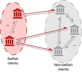
Our work: In this work, we show that the decentralized nature of DFL makes it vulnerable to a unique family of attacks which we call SelfishAttack. In SelfishAttack, a set of clients called selfish clients collusively compromise the DFL training process to achieve two goals: 1) their final learnt local models are more accurate than those learnt via DFL solely among the selfish clients themselves (called utility goal), and 2) their final learnt local models are more accurate than those of the remaining non-selfish clients (called competitive-advantage goal). The utility goal means that, by joining the DFL training process, the selfish clients can learn more accurate local models; while the competitive-advantage goal aims to gain competitive advantages over non-selfish clients.
For instance, suppose multiple banks use DFL to train local models for financial fraud detection. A set of collusive selfish banks can use SelfishAttack to compromise the DFL training process so 1) they can still learn more accurate local models than DFL solely among themselves, and 2) their final learnt local models can detect financial frauds much more accurately than those of the non-selfish banks, gaining competitive advantages. To achieve the goals, SelfishAttack carefully crafts shared models sent from the selfish clients to the non-selfish ones in each global training round. Note that a selfish client still sends its pre-aggregation local model as shared model to other selfish clients, while a non-selfish client still sends its pre-aggregation local model as shared model to other clients.
Our SelfishAttack is qualitatively different from conventional poisoning attacks to CFL/DFL [3, 7, 10] with respect to both threat models and technical approaches. For threat model, poisoning attacks assume an external attacker who has control over some compromised genuine clients [3, 10] or injected fake clients [7], while SelfishAttack considers an internal attacker (i.e., insider of DFL) that consists of multiple selfish clients. Moreover, the goal of a conventional poisoning attack is that a poisoned model (e.g., poisoned local model of a non-selfish client when extended to our problem setting) misclassifies a large fraction of clean inputs indiscriminately.111These are known as untargeted poisoning attacks. We also discuss targeted poisoning attacks in Section 2.2. In contrast, SelfishAttack aims to increase the accuracy gap between selfish clients and non-selfish ones while guaranteeing that the selfish clients still learn more accurate local models by joining the DFL process.
Poisoning attacks can be extended to gain competitive advantages (i.e., achieve the competitive-advantage goal) as follows: 1) a selfish client uses a conventional poisoning attack to craft shared models sent to the non-selfish clients so their learnt local models are inaccurate, and 2) the selfish clients only use their own shared models for aggregation so their local models are not influenced by the non-selfish clients’ inaccurate shared models, which is equivalent to performing DFL among the selfish clients themselves. However, as our experiments in Section 5.2 show, such attack cannot achieve the utility goal. This is because selfish clients do not leverage any information of the non-selfish clients for aggregation.
Since the threat models are different, our SelfishAttack and conventional poisoning attacks also use substantially different technical approaches. Specifically, when extended to our problem setting, a conventional poisoning attack aims to craft shared models sent from selfish clients to a non-selfish one to deviate its post-aggregation local model the most in each global training round. In contrast, we formulate SelfishAttack as an optimization problem, which aims to minimize a weighted sum of two loss terms that respectively quantify two attack goals. Specifically, to achieve the utility goal, we aim to craft shared models sent from selfish clients to a non-selfish one such that its post-aggregation local model is close to its pre-aggregation one in a global training round. Therefore, the non-selfish client still sends a useful shared model to selfish clients in the next global training round, and selfish clients can leverage non-selfish clients’ shared models to improve their local models. Formally, we quantify the utility goal by treating the Euclidean distance between the post-aggregation local model and the pre-aggregation one of a non-selfish client as a loss term. Moreover, to achieve the competitive-advantage goal, we aim to deviate the post-aggregation local model of a non-selfish client. Formally, we quantify the competitive-advantage goal by treating the Euclidean distance between the post-aggregation local model after attack and the one before attack of a non-selfish client as the other loss term.
In a global training round, the selfish clients solve the optimization problem to craft the shared models sent to each non-selfish client. First, we derive the analytical form of the optimal post-aggregation local model for each non-selfish client that minimizes the weighted sum of the two loss terms. Second, for aggregation rules such as FedAvg [18], Median [25], and Trimmed-mean [25], we further derive the analytical form of the shared models sent from the selfish clients to each non-selfish one such that its post-aggregation local model becomes the optimal one. In other words, when the non-selfish clients use these aggregation rules, we can derive the analytical form of the optimal shared models sent from selfish clients to non-selfish ones to achieve a desired trade-off between the two attack goals, which is quantified by a weighted sum of the two loss terms. When the non-selfish clients use other aggregation rules such as Krum [4], FLTrust [6], FLDetector [26], and FLAME [19], it is hard to derive the analytical form of the optimal shared models. To address the challenge, the selfish clients use the optimal shared models derived for FedAvg, Median, or Trimmed-mean to attack them.
We evaluate our SelfishAttack on three datasets (CIFAR-10, FEMNIST, and Sent140) from different domains and extend poisoning attacks to our problem setting. Our results show that SelfishAttack can achieve the two attack goals. For instance, on CIFAR-10 dataset and when 30% of clients are selfish, the final learnt local models of the selfish clients are at least 11% more accurate than those of the non-selfish ones under SelfishAttack. Moreover, compared to conventional poisoning attacks, SelfishAttack learns more accurate local models for the selfish clients (i.e., better achieves the utility goal) and/or achieves a larger accuracy gap between the local models of the selfish clients and those of the non-selfish ones (i.e., better achieves the competitive-advantage goal).
Our contributions can be summarized as follows:
-
•
We propose SelfishAttack, a new family of attacks to DFL, in which selfish clients aim to increase the competitive advantages over non-selfish ones while maintaining the utility of their local models.
-
•
We derive analytical forms of the optimal shared models that the selfish clients should send to the non-selfish ones in order to achieve a desired trade-off between the two attack goals, when the non-selfish clients use aggregation rules including FedAvg, Median, or Trimmed-mean.
-
•
We extensively evaluate SelfishAttack and compare it with poisoning attacks using three benchmark datasets. Our results show that SelfishAttack achieves the two attack goals and outperforms poisoning attacks.
2 Preliminaries and Related Work
2.1 Decentralized Federated Learning
Consider a decentralized federated learning (DFL) system with clients. Each client has a local training dataset , where . These clients collaboratively train a machine learning model without the reliance of a central server. In particular, DFL aims to find a model that minimizes the weighted average of losses among all clients:
| (1) |
where is the local training objective of client , is the number of training examples of client , and is the dimension of model . In each global training round , DFL performs the following three steps:
-
•
Step I. Every client trains a local model using its own local training dataset. Specifically, for client , it samples a mini-batch of training examples from its local training dataset, and calculates a stochastic gradient . Then, client updates its local model as , where represents the learning rate, is the local model of client at the beginning of the -th global training round, and is the pre-aggregation local model of client at global training round . Note that client can compute stochastic gradient and update its local model multiple times in each global training round.
-
•
Step II. Client sends a shared model to each client and also receives a shared model from each client , where and . In non-adversarial settings, the shared model is the pre-aggregation local model of client , i.e., . Our SelfishAttack carefully crafts the shared models sent from selfish clients to non-selfish ones.
-
•
Step III. Client aggregates the clients’ shared models and updates its local model as , where denotes an aggregation rule and is the post-aggregation local model of client . Note that we assume for .
DFL repeats the above iterative process for multiple global training rounds. Different DFL methods use different aggregation rules, such as FedAvg [17] and Median [25]. Note that in non-adversarial settings, all clients have the same post-aggregation local model in each global training round. Table 5 in Appendix summarizes the key notations used in our paper.
2.2 Poisoning Attacks to CFL/DFL
Conventional poisoning attacks to FL can be divided into two categories depending on the goal of the attacker, namely untargeted attacks [3, 10] and targeted attacks [1, 2]. These poisoning attacks were originally designed for CFL, but they can be extended to our problem setting. Specifically, an untargeted attack aims to manipulate the DFL system such that a poisoned local model of a non-selfish client produces incorrect predictions for a large portion of clean testing inputs indiscriminately, i.e., the final learnt local model of a non-selfish client has a low testing accuracy. For instance, in Gaussian attack [3], each selfish client sends an arbitrary Gaussian vector to non-selfish clients; while Trim attack [10] carefully crafts the shared models sent from selfish clients to non-selfish ones in order to significantly deviate non-selfish clients’ post-aggregation local models in each global training round. A targeted attack [1, 2] aims to poison the system such that the local model of a non-selfish client predicts a predefined label for the inputs that contain special characteristics such as those embedded with predefined triggers.
Note that our SelfishAttack differs from these poisoning attacks in the following two dimensions. First, conventional poisoning attacks assume that an external attacker controls some compromised genuine clients or injected fake clients. In contrast, in our attack, we consider an internal attacker composed of several selfish clients. Second, conventional poisoning attacks focus on degrading the performance of final learned local models of non-selfish clients on either indiscriminate testing inputs or inputs with certain characteristics. In contrast, in our SelfishAttack, selfish clients aim to gain competitive advantages over non-selfish clients while maintaining the utility of their local models. Even though we can adapt the conventional poisoning attacks to our context (e.g., gain competitive advantages), they cannot achieve satisfying performance as evidenced by our experiments.
2.3 Byzantine-robust Aggregation Rules
The FedAvg [17] aggregation rule is commonly used in non-adversarial settings. However, a single shared model can arbitrarily manipulate the post-aggregation local model of a non-selfish client in FedAvg [3]. Byzantine-robust aggregation rules [3, 6, 19, 25] aim to be robust against “outlier” shared models when applied to DFL. In particular, when a non-selfish client uses a Byzantine-robust aggregation rule, its post-aggregation local model is less likely to be influenced by outlier shared models, e.g., those from selfish clients.
For instance, Median [25] and Trimmed-mean [25] are two coordinate-wise aggregation rules, which remove the outliers in each dimension of clients’ shared models in order to reduce the impact of outlier shared models. Specifically, for a given client, the Median aggregation rule outputs the coordinate-wise median of the client’s received shared models as the post-aggregation local model. For each dimension, the Trimmed-mean aggregation rule first removes the largest and smallest elements, then takes the average of the remaining items, where is the trim parameter. Krum [3] aggregates a client’s received shared models by selecting the shared model that has the smallest sum of Euclidean distance to its subset of neighboring shared models. We note that the previous work [9] has already applied Median, Trimmed-mean, and Krum aggregation rules in the context of DFL. In FLTrust [6], if a received shared model diverges significantly from the pre-aggregation local model of client , then client assigns a low trust score to this received shared model. In FLDetector [26], clients leverage clustering techniques to detect outlier shared models and then aggregate shared models from clients that have been detected as non-selfish. In FLAME [19], clients leverage clustering and model weight clipping techniques to mitigate the impact of outlier shared models.
3 Threat Model
Attacker’s goal: We consider a collusive set of selfish clients to be an attacker. The selfish clients aim to compromise the integrity of the DFL training process to achieve two goals: utility goal and competitive-advantage goal. The utility goal means that, by joining the collaborative DFL training process with the non-selfish clients, the selfish clients can learn more accurate local models. Suppose is the local model of a selfish client learnt by joint DFL training among the selfish clients themselves, i.e., the selfish clients do not collaborate with the non-selfish ones. Moreover, is the local model of the selfish client learnt by joint DFL training among the selfish and non-selfish clients. The utility goal means that should be more accurate than .
The competitive-advantage goal means that the local models of the selfish clients are more accurate than those of the non-selfish clients. This goal gives competitive advantages to the selfish clients. In particular, with more accurate local models, the selfish clients (e.g., banks or hospitals) could attract more customers and make more revenues.
Attacker’s capabilities: A selfish client sends its pre-aggregation local model as a shared model to other selfish clients. However, a selfish client can arbitrarily manipulate the shared models sent to non-selfish clients. Note that a non-selfish client sends its pre-aggregation local model as a shared model to other clients in each global training round. Following the standard assumption in distributed systems [15], we assume , where is the number of selfish clients and is the total number of clients. Fig. 1 illustrates our SelfishAttack.
Attacker’s background knowledge: The selfish clients know the aggregation rule of the DFL system as they are a part of the system. Moreover, they know the pre-aggregation local models of non-selfish clients in each global training round since the non-selfish clients send them as shared models to selfish clients. The selfish clients also know each other’s pre-aggregation local models since they exchange them.
4 Our SelfishAttack
4.1 Overview
We formulate SelfishAttack as an optimization problem that minimizes a weighted sum of two loss terms quantifying the two attack goals respectively. The first loss term quantifies the utility goal, which aims to create shared models sent from selfish clients to a non-selfish client, ensuring that its post-aggregation local model remains close to its pre-aggregation local model. The second loss term quantifies the competitive-advantage goal, which aims to deviate the post-aggregation local model of a non-selfish client. However, the optimization problem is hard to solve because its objective function is non-differentiable with respect to the shared models. To address the challenge, we first derive the optimal post-aggregation local model of a non-selfish client that minimizes the objective function. Then, for aggregation rules such as FedAvg, Median, and Trimmed-mean, we propose methods to craft the shared models sent from selfish clients to a non-selfish client, such that the non-selfish client’s post-aggregation local model becomes the optimal one. In other words, our crafted shared models are optimal for these aggregation rules. When the DFL system uses other aggregation rules, selfish clients can employ the optimal shared models derived based on FedAvg, Median, or Trimmed-mean to attack them. Finally, we propose a method for the selfish clients to determine when to start attack.
4.2 Formulating an Optimization Problem
We assume that there are non-selfish clients and selfish clients in the DFL system. We denote a non-selfish client as and a selfish client as , where and . Recall that is the pre-aggregation local model of non-selfish client in global training round . Our SelfishAttack performs attack in different global training rounds separately. Therefore, in the following, we ignore the superscripts and in our notations for simplicity. Moreover, we denote by the post-aggregation local model of a non-selfish client in global training round .
Quantifying the utility goal: The utility goal means that the selfish clients can learn more accurate local models via DFL with non-selfish clients. In other words, the shared models sent from non-selfish clients to the selfish clients should still include useful information that can be used to improve selfish clients’ local models. To achieve this goal, the selfish clients aim to craft shared models sent to a non-selfish client such that its post-aggregation local model is close to its pre-aggregation local model . The intuition is that the pre-aggregation local model includes useful information about the local training data of client . When the post-aggregation local model is close to in global training round , client can learn a good pre-aggregation local model in the next global training round and send it to selfish clients, which can further leverage it to improve their local models. Formally, we quantify the utility goal as a loss term that is the square of Euclidean distance between and , i.e., , where means Euclidean distance.
Quantifying the competitive-advantage goal: The competitive-advantage goal means that selfish clients can learn more accurate local models than non-selfish clients. To achieve this goal, we aim to decrease the accuracy of the non-selfish clients’ local models. We denote by the post-aggregation local model of client if only the non-selfish clients’ shared models are used for aggregation. represents the post-aggregation local model that client can have if there are no selfish clients. To achieve the competitive-advantage goal, the selfish clients aim to craft shared models such that the post-aggregation local model of client deviates substantially from , making less accurate. Formally, we quantify the competitive-advantage goal as a loss term that is the negative square of Euclidean distance between and , i.e., .
Optimization problem: After quantifying both attack goals, we can combine them as an optimization problem. Formally, we have the following:
| s.t. | ||||
| (2) |
where denotes the aggregation rule, is the crafted shared model sent from selfish client () to non-selfish client , the first loss term in the objective function quantifies the utility goal, the second loss term in the objective function quantifies the competitive-advantage goal, and is a hyperparameter to achieve a trade-off between the two attack goals. Note that our formulation is a general framework and can be applied to any aggregation rule .
4.3 Solving the Optimization Problem
Solving the optimization problem in Equation 4.2 is not trivial because the objective function is not differentiable with respect to the shared models when the aggregation rule is complex such as Median, Trimmed-mean, and FLTrust. To address the challenge, we transform the optimization problem to one whose variable is the post-aggregation local model . Then, we derive the optimal solution to the transformed optimization problem. Finally, for coordinate-wise aggregation rules including FedAvg, Median, and Trimmed-mean, we derive the optimal shared models that achieve the optimal solution . When the non-selfish clients use other aggregation rules, the selfish clients use the optimal shared models derived for FedAvg, Median, or Trimmed-mean to attack them.
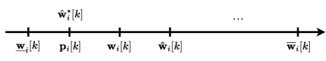
Transformed optimization problem: Note that , where denotes the transpose of . For simplicity, we define two -dimension vectors, and , such that for each dimension , is lower bounded by and upper bounded by , i.e., , where . We reformulate the optimization problem in Equation 4.2 as follows for each , where :
| s.t. | (3) |
Optimal solution of the transformed optimization problem: Equation 4.3 is a standard quadratic optimization problem, which is constrained within the interval . For convenience, we denote by a vector with dimensions, each dimension of which satisfies the following:
| (4) |
where . Let represent a -dimension vector, and its -th dimension is the optimal solution of Equation 4.3. We can solve separately in the following three cases:
Case I: . In this case, if is within the interval , then the optimal solution is . Otherwise, we have if is larger than ; and if is smaller than . In other words, we have the following:
| (5) |
Case II: . In this case, we have as follows:
| (6) |
Case III: . In this case, is a value between and that has the larger distance to . That is, we have the following:
| (7) |
Fig. 2 shows an example of the optimal solution when (Case I and ). Next, we demonstrate that when a client uses the FedAvg, Median, or Trimmed-mean aggregation rule, selfish clients can craft the shared models such that the -th dimension of the post-aggregation local model of client is , i.e., . Specifically, for each of the three aggregation rules, we first show how to determine the lower/upper bounds and , then derive the analytical forms of the shared models , and finally prove that the derived shared models are optimal solutions of the original optimization problem in Equation 4.2.
4.4 Attacking FedAvg
Determining and : Since FedAvg is not a Byzantine-robust aggregation rule, we can craft shared models to make reach any desired value. However, to avoid being easily detected, we assume an upper bound and a lower bound for . Specifically, we assume that and .
Crafting shared models of selfish clients: Since we have determined and , we can compute based on Equations 5-7. Recall that FedAvg takes the average of all shared models in each dimension . In order to make the post-aggregation local model of client be the optimal solution of Equation 4.3, one way is to fix values in , and then adjust the value of the remaining one. For simplicity, we set the values of to be the same as , and calculate the corresponding value of so that the average value of is . To be more specific, we have the following:
| (8) | ||||
Optimality of the crafted shared models: The following Theorem 1 shows that the crafted shared models in Equation 8 satisfy , which means that the crafted shared models are optimal solutions of Equation 4.2.
Theorem 1.
Proof.
Please see Appendix A.1. ∎
4.5 Attacking Median
Determining and : For convenience, we sort the scalar values in a descending order, and we denote the sorted sequence as , i.e., we have . Since Median discards the outliers in each dimension of the shared models and , we have that has a lower and upper bound. Suppose we are given a sorted sequence with values . If we append values to this sequence, the resulting median is maximized if the added values are larger than . Thus, the maximum value of , denoted as , can be determined as the following:
| (9) |
Similarly, the median is minimized if all the added values are smaller than . Therefore, we can compute the minimum value of , represented as , as follows:
| (10) |
Crafting shared models of selfish clients: Once we have obtained and , we can calculate using Equations 5-7. It is important to note that is the pre-aggregation local model and is defined in Equation 4. Both and are independent of . Then, we craft selfish clients’ shared models based on . To ensure that the post-aggregation local model of a non-selfish client satisfies , one straightforward approach is to assign the values of to be identical to . However, there is one scenario where the above straightforward approach does not apply. It occurs when the total number of clients is even and the value of falls into the interval or , where and . In this exception case, we either have or , which is not . To take this exception case into consideration and ensure that , we determine the value of based on the following three cases:
| (11) |
After calculating the value of using Equation 11, we assign the same value of to , i.e., we have:
| (12) |
where is defined as follows:
| (13) |
where is a constant.
Optimality of the crafted shared models: The following Theorem 2 shows that the crafted shared models in Equations 11-13 satisfy , which means that the crafted shared models are optimal solutions of Equation 4.2.
Theorem 2.
Proof.
Please see Appendix A.2. ∎
4.6 Attacking Trimmed-mean
Determining and : In Trimmed-mean, for every dimension , a client first removes the largest and smallest elements, and then takes the average of the remaining values. We assume that is equal to the number of selfish clients, i.e., , which gives advantages to non-selfish clients. For convenience, for the -th dimension, we also use a sorted sequence to represent the sorted model parameters of non-selfish clients. The sorted sequence satisfies . Given our threat model that the number of selfish clients is less than one-third of the total number of clients , when a non-selfish client uses the Trimmed-mean aggregation rule to aggregate the shared models, the resulting post-aggregation local model has a lower and upper bound. To be specific, suppose values are added to the sorted sequence . If these values are greater than , the resulting trimmed mean value reaches the maximum value. Therefore, the maximum value of , denoted as , can be computed as follows:
| (14) |
Likewise, when the added values are less than , the resulting trimmed mean value reaches its minimum. Thus, the minimum value of , denoted as , can be calculated as follows:
| (15) |
Crafting shared models of selfish clients: After determining the values of and , we can compute by Equations 5-7. We then further craft selfish clients’ shared models using . Our main idea is that we intentionally allow non-selfish client to exclude certain shared model parameters received from selfish clients while calculating the trimmed mean value. Afterwards, we carefully craft the remaining model parameters from selfish clients such that the average value of the remaining elements becomes . Specifically, we consider two cases as follows:
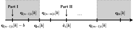
Case I: . In this case, the post-aggregation local model is not larger than , which is the trimmed mean value of the -th dimensional parameters of all non-selfish clients’ shared models. We aim to add values into the sorted sequence , such that the resulting trimmed mean value decreases from to . In our attack, we set a part of the shared model parameters sent by selfish clients to be less than (we refer to this part as Part I selfish model parameters), while adjusting the values of the remaining part (called Part II selfish model parameters). Note that we also need to make sure that when calculating the trimmed-mean value of , the Part II selfish model parameters remain unfiltered. This can be achieved by adding some conditions on the number of Part I selfish model parameters. Suppose that there are Part I selfish model parameters, where , and at the same time is the largest integer that satisfies the following condition:
| (16) |
If , there are no Part II selfish model parameters. Then we can set as follows:
| (17) |
where is a positive constant. If , we have Part II selfish model parameters. Then we craft the corresponding values of these Part II selfish model parameters so that the trimmed-mean value of is equal to . In particular, we can set the following:
| (18) |
where is computed as:
| (19) |
In other words, we set the values of Part I selfish model parameters as , and Part II selfish model parameters as . Fig. 3 shows an example of this case.
Case II: . In this case, the post- aggregation local model is larger than . Similar to Case I, we set a part of the shared model parameters to be larger than (Part I selfish model parameters), while adjusting the values of the remaining parts (we call Part II selfish model parameters). Suppose that the number of Part I selfish model parameters is , where and is also the smallest integer that satisfies the following:
| (20) |
If , there are no Part II selfish model parameters. can be set as follows:
| (21) |
where is a positive constant. If , we have Part II selfish model parameters. We can craft as the following:
| (22) |
where is computed as:
| (23) |
To summarize, we set Part I selfish model parameters as and Part II selfish model parameters as .
Optimality of the crafted shared models: The following Theorem 3 shows that the crafted shared models satisfy , which means that the crafted shared models are optimal solutions of Equation 4.2.
Theorem 3.
Proof.
Please see Appendix A.3. ∎
4.7 Attacking other Aggregation Rules
When the aggregation rule is coordinate-wise FedAvg, Median, or Trimmed-mean, we can derive the optimal shared models sent by selfish clients to non-selfish ones. However, it is hard to derive the optimal shared models to attack other non-coordinate-wise aggregation rules such as Krum [4], FLTrust [6], FLDetector [26], and FLAME [19]. To attack such aggregation rules, the selfish clients can use the shared models crafted based on FedAvg, Median, or Trimmed-mean (we use FedAvg in experiments). Moreover, we tailor our attack to FLAME as detailed in Appendix A.4. Although such attack may not be optimal for other aggregation rules, our empirical results indicate that it can achieve decent effectiveness. Note that selfish clients know the aggregation rule adopted by the DFL, so they can decide which method should be used to craft the shared models sent to non-selfish clients.
4.8 When to Start Attack
Intuitively, if selfish clients start to attack at the very beginning global training rounds, the non-selfish clients may not be able to learn good local models. As a result, the selfish clients cannot obtain useful information from the shared models sent by non-selfish clients, making it hard to achieve the utility goal. Therefore, we design a mechanism for the selfish clients to determine when to start attack. Our key idea is that the selfish clients start to attack in the global training rounds when clients have obtained decent local models.
Specifically, in addition to shared model, each selfish client also sends its local training loss to other selfish clients in global training round . Once selfish client receives the losses from other selfish clients, it calculates the average of these losses and obtains the minimum value among all previous global training rounds. Then, selfish client compares the decrease in over the past global training rounds with the maximum decrease in this average value across all global training rounds. When the ratio of the former to the latter is less than a threshold , the selfish clients start to attack, i.e., send carefully crafted shared models to non-selfish clients in future global training rounds. This is because the clients’ local training losses start to change slowly and the clients have probably obtained descent local models. Note that we have two hyper-parameters, and , to control when to initiate the attack. We will explore the impact of these two hyper-parameters on our attack in experiments in Section 4.
4.9 Complete Algorithm of SelfishAttack
Algorithm 1 in Appendix summarizes our SelfishAttack. Specifically, lines 6 to 8 describe Step I of DFL, where each client performs local training of its pre-aggregation local model. Lines 9 to 14 illustrate the process of exchanging shared models among clients in the global training rounds before our attack starts. Lines 17 to 23 provide a detailed description of Section 4.8, explaining how to determine when to start attack. The process of performing attack is shown in lines 24 and 25, while the methods of crafting shared models are presented in Algorithm 2 in Appendix.
5 Evaluation
5.1 Experimental Setup
Datasets: We evaluate our proposed SelfishAttack on three benchmark datasets, including two image classification datasets and one text classification dataset.
CIFAR-10 [14]. CIFAR-10 is a 10-class color image classification dataset, which contains 50,000 training examples and 10,000 testing examples.
Federated Extended MNIST (FEMNIST) [5]. FEMNIST is a 62-class image classification dataset. It is constructed by partitioning the data from Extended MNIST [16] based on the writer of the digit or character. There are 3,550 writers and 805,263 examples in total. To distribute the training examples to clients, we select 10 writers for each client and combine their data as the local training data for a client.
Sentiment140 (Sent140) [11]. Sent140 is a two-class text classification dataset for sentiment analysis. The data are tweets collected from 660,120 twitter users and annotated based on the emoticons present in themselves. In our experiments, we choose 300 users with at least 10 tweets for each client, and the union of the training tweets of these 300 users is the client’s local training data.
| Method | FedAvg | Median | Trimmed-mean | ||||||
| MTAS | MTANS | Gap | MTAS | MTANS | Gap | MTAS | MTANS | Gap | |
| No attack | 0.627 | 0.627 | 0.000 | 0.644 | 0.644 | 0.000 | 0.644 | 0.644 | 0.000 |
| Independent | 0.321 | 0.307 | 0.014 | 0.321 | 0.307 | 0.014 | 0.321 | 0.307 | 0.014 |
| Two Coalitions | 0.505 | 0.578 | -0.073 | 0.505 | 0.578 | -0.073 | 0.505 | 0.578 | -0.073 |
| TrimAttack | 0.207 | 0.165 | 0.043 | 0.524 | 0.513 | 0.011 | 0.456 | 0.440 | 0.016 |
| GaussianAttack | 0.098 | 0.089 | 0.008 | 0.619 | 0.617 | 0.001 | 0.613 | 0.609 | 0.004 |
| SelfishAttack | 0.475 | 0.326 | 0.150 | 0.543 | 0.425 | 0.119 | 0.597 | 0.484 | 0.113 |
| Method | FedAvg | Median | Trimmed-mean | ||||||
| MTAS | MTANS | Gap | MTAS | MTANS | Gap | MTAS | MTANS | Gap | |
| No attack | 0.790 | 0.790 | 0.000 | 0.791 | 0.791 | 0.000 | 0.795 | 0.795 | 0.000 |
| Independent | 0.543 | 0.545 | -0.002 | 0.543 | 0.545 | -0.002 | 0.543 | 0.545 | -0.002 |
| Two Coalitions | 0.755 | 0.784 | -0.029 | 0.755 | 0.784 | -0.029 | 0.755 | 0.784 | -0.029 |
| TrimAttack | 0.056 | 0.055 | 0.001 | 0.751 | 0.741 | 0.010 | 0.744 | 0.736 | 0.008 |
| GaussianAttack | 0.003 | 0.028 | -0.025 | 0.788 | 0.785 | 0.003 | 0.793 | 0.789 | 0.003 |
| SelfishAttack | 0.697 | 0.575 | 0.123 | 0.771 | 0.643 | 0.128 | 0.792 | 0.747 | 0.045 |
| Method | FedAvg | Median | Trimmed-mean | ||||||
| MTAS | MTANS | Gap | MTAS | MTANS | Gap | MTAS | MTANS | Gap | |
| No attack | 0.791 | 0.791 | 0.000 | 0.824 | 0.824 | 0.000 | 0.788 | 0.788 | 0.000 |
| Independent | 0.631 | 0.637 | -0.006 | 0.631 | 0.637 | -0.006 | 0.631 | 0.637 | -0.006 |
| Two Coalitions | 0.751 | 0.791 | -0.039 | 0.751 | 0.791 | -0.039 | 0.751 | 0.791 | -0.039 |
| TrimAttack | 0.740 | 0.715 | 0.025 | 0.760 | 0.763 | -0.003 | 0.771 | 0.765 | 0.006 |
| GaussianAttack | 0.536 | 0.528 | 0.008 | 0.807 | 0.807 | 0.000 | 0.785 | 0.785 | 0.000 |
| SelfishAttack | 0.799 | 0.647 | 0.152 | 0.804 | 0.683 | 0.121 | 0.816 | 0.730 | 0.085 |
Aggregation rules: A client can use different aggregation rules to aggregate the clients’ shared models as a post-aggregation local model. We evaluate the following aggregation rules.
FedAvg [18]. In FedAvg, a client aggregates the received shared models by calculating their average.
Median [25]. Each client in Median obtains the post-aggregation local model via taking the coordinate-wise median of the shared models.
Trimmed-mean [25]. Trimmed-mean is another coordinate-wise method that calculates the trimmed mean value of the shared models in each dimension. Specifically, for a given dimension , each client first removes the largest and smallest values, then computes the average of the remaining elements. In our experiments, we set , where is the number of selfish clients, giving advantages to this aggregation rule.
Krum [4]. In Krum aggregation rule, each client outputs one shared model that has the smallest sum of Euclidean distances to its closest neighbors.
FLTrust [6]. In FLTrust, client computes a trust score for each received shared model in each global training round, where . A shared model has a lower trust score if it deviates more from the pre-aggregation local model of client . Client then computes the weighted average of the received shared models, where the weights are determined by their respective trust scores.
FLDetector [26]. In FLDetector, client predicts a client’s shared model updates based on its historical information in each training round and identifies a client as selfish when the predicted model updates consistently deviate from the shared model updates calculated by the received shared model across multiple training rounds. Then client employs the Median aggregation rule to combine the predicted non-selfish clients’ shared models.
FLAME [19]. FLAME uses a clustering-based method to detect and eliminate bad shared models. Additionally, it uses dynamic weight-clipping to further reduce the impact of shared models potentially from selfish clients.
Compared methods: We compare our proposed SelfishAttack with the following methods.
Independent. Independent means each client independently trains a local model using its own local training dataset without DFL.
Two Coalitions. This method divides the clients into two coalitions: selfish clients and non-selfish clients. Clients within the same coalition collaborate using DFL with the FedAvg aggregation rule. This scenario means that selfish clients do not join DFL together with non-selfish clients.
TrimAttack [10]. TrimAttack was originally designed as a local model poisoning attack to CFL. We extend it to our problem setting. Specifically, selfish clients use TrimAttack to craft shared models sent to non-selfish clients such that the post-aggregation local model after attack deviates substantially from the one before attack, in terms of both direction and magnitude.
GaussianAttack [3]. In GaussianAttack, a selfish client sends a random Gaussian vector as a shared model to a non-selfish client. Each dimension of the Gaussian vector is generated from a normal distribution with zero mean and standard deviation 200.
DFL parameter settings: By default, we assume 20 clients in total, including 6 (30%) selfish clients and 14 non-selfish clients. We train a CNN classifier for each client on CIFAR-10 dataset. We also train a CNN classifier for the FEMNIST dataset. We train a LSTM [13] classifier for the Sent140 dateset. The CNN architectures for CIFAR-10 and FEMNIST datasets are shown in Table 7 and 8 in Appendix, respectively. The LSTM architecture for Sent140 dataset is shown in Table 9 in Appendix. Table 6 in Appendix summarizes the DFL parameter settings for the three datasets.
In DFL, the clients’ local training data are typically not independent and identically distributed (Non-IID). We adopt the approach in [10] to simulate the Non-IID setting for CIFAR-10 dataset. Specifically, we randomly split all clients into 10 groups. We use a probability to assign a training example with label to the clients in one of these 10 groups. Specifically, the training example with label is assigned to clients in group with a probability of , and to clients in any other groups with the same probability of , where . Within the same group, the training example is uniformly distributed among the clients. The parameter controls the degree of Non-IID. The local training data are IID distributed when , otherwise the training data are Non-IID distributed. A larger value of implies a higher degree of Non-IID. By default, we set for CIFAR-10 dataset. Note that the clients’ local training data in FEMNIST and Sent140 datasets are already Non-IID. Thus, there is no need to simulate Non-IID for FEMNIST and Sent140 datasets.
Parameter settings for SelfishAttack: By default, we set when attacking FedAvg; and when attacking Median; and when attacking Trimmed-mean. We adopt different for different aggregation rules because they aggregate shared models differently. Note that the selfish clients know the aggregation rule used by the DFL, and thus they can set accordingly. We set and across different aggregation rules. Unless otherwise mentioned, we report the experimental results on CIFAR-10 dataset for simplicity. By default, we assume that a selfish client uses the same aggregation rule adopted by the DFL and all the clients’ shared models for aggregation. However, we will also explore the scenarios where selfish clients use a different aggregation rule and/or only their own shared models for aggregation.
Evaluation metrics: We evaluate the performance of SelfishAttack and other compared attacks using three metrics: mean testing accuracy of selfish clients (MTAS), mean testing accuracy of non-selfish clients (MTANS), and the Gap between them, i.e., Gap=MTAS-MTANS. MTAS (or MTANS) is the mean testing accuracy of the local models of the selfish (or non-selfish) clients. We note that, under attacks, the selfish clients have the same final local model, while the non-selfish ones may have different final local models.
5.2 Experimental Results
SelfishAttack achieves the two attack goals: Table 1c show the results of SelfishAttack and other compared attacks under different aggregation rules and different datasets. “No attack” means selfish clients do not launch any attacks and just send their pre-aggregation local models as shared models to non-selfish clients. Our results demonstrate that SelfishAttack achieves the utility and competitive-advantage goals.
First, we observe that the final learnt local models of selfish clients under SelfishAttack are more accurate when they collaborate with the non-selfish clients, compared to when they engage in DFL solely among themselves. This demonstrates that our proposed SelfishAttack achieves the utility goal. For instance, the MTASs of Median and Trimmed-mean aggregation rules under SelfishAttack are larger than those of Two Coalitions on all three datasets. Note that we do not have this observation for FedAvg and CIFAR-10/FEMNIST dataset. This is because FedAvg is not robust, in which the post-aggregation local models of non-selfish clients are negatively influenced by the shared models from selfish clients too much.
Second, we observe that our proposed SelfishAttack can effectively increase the gap between the mean accuracy of selfish clients and that of non-selfish clients, indicating that SelfishAttack achieves the competitive-advantage goal. In particular, the Gap of SelfishAttack is greater than in most cases. Take CIFAR-10 dataset as an example, the Gaps are , , and when the aggregation rule is FedAvg, Median, and Trimmed-mean, respectively. When the aggregation rule is Trimmed-mean and dataset is FEMNIST or Sent140, the Gaps are smaller than , but they are still and , respectively.
Third, our SelfishAttack consistently outperforms compared attacks across all three datasets and aggregation rules. The Gap of TrimAttack is less than or close to in most cases. The Gap of TrimAttack is even negative when attacking Median on Sent140 dataset. Similarly, the Gap of GaussianAttack remains below in all cases. SelfishAttack outperforms GaussianAttack because the latter is ineffective against robust aggregation rules such as Median and Trimmed-mean. Additionally, when FedAvg is used, the MTAS of GaussianAttack is also very low, resulting in a low Gap. SelfishAttack outperforms TrimAttack because the selfish clients can still leverage useful information in the shared models from the non-selfish clients to improve their local models in SelfishAttack. In contrast, a non-selfish client obtains an inaccurate local model in TrimAttack and further sends the inaccurate shared model to selfish clients. As a result, both non-selfish and selfish clients have inaccurate local models, leading to smaller GAPs.
| Attacks | Info. | MTAS | MTANS | Gap |
| TrimAttack | All | 0.456 | 0.440 | 0.016 |
| Selfish | 0.540 | 0.440 | 0.100 | |
| GaussianAttack | All | 0.613 | 0.609 | 0.004 |
| Selfish | 0.540 | 0.609 | -0.069 | |
| SelfishAttack | All | 0.597 | 0.484 | 0.113 |
| Selfish | 0.540 | 0.484 | 0.057 |
Using all clients’ shared models vs. selfish clients’ ones for aggregation: By default, in Step III of DFL, we assume that a selfish client aggregates the shared models sent from both selfish and non-selfish clients. However, we observe from Table 1c that when selfish clients craft the shared models using existing attacks (e.g., TrimAttack or GaussianAttack), the testing accuracy of the selfish clients’ local models is also influenced as well. This is because non-selfish clients are unable to obtain accurate local models under these attacks. As a result, when selfish clients take into account the shared models of non-selfish clients during the aggregation process, they also fail to obtain accurate local models. Therefore, selfish clients can choose to only use the shared models from selfish clients for aggregation in order to enhance their own testing accuracy. In Table 2, “All" or “Selfish" means that when performing aggregation, selfish clients use the shared models of all clients or only the selfish clients. Specifically, selfish clients use the FedAvg aggregation rule to enhance testing accuracy, while non-selfish clients employ the Trimmed-mean aggregation rule to enhance robustness.
We observe that our attack achieves a larger Gap when the selfish clients use all clients’ shared models for aggregation. This is because non-selfish clients still contribute to the local models of selfish clients under our SelfishAttack. However, TrimAttack achieves a larger Gap when the selfish clients only use the selfish clients’ shared models for aggregation, compared to using all clients’ shared models for aggregation. The reason is that the non-selfish clients contribute negatively to the local models of the selfish clients under TrimAttack. Overall, the best attack strategy for selfish clients is to use SelfishAttack to craft the shared models sent to the non-selfish clients and use all clients’ shared models for aggregation.
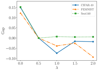
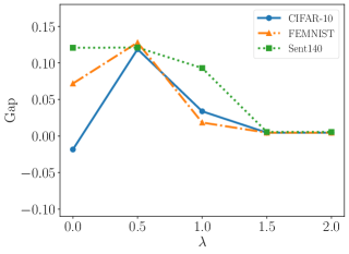
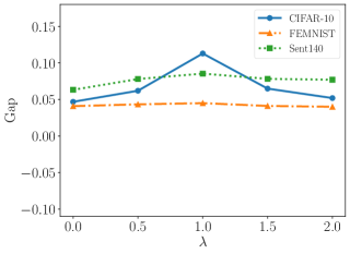
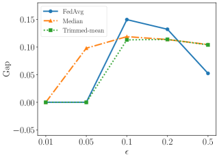
Impact of : Fig. 4 shows the impact of on Gap of SelfishAttack when DFL uses different aggregation rules. We observe that for robust aggregation rules like Median and Trimmed-mean, GAP tends to increase as increases. However, once surpasses a certain threshold (e.g., 0.5 for Median and 1.0 for Trimmed-mean), GAP begins to decline. This is because a larger places more emphasis on the competitive-advantage goal, as defined in Equation 4.2. Consequently, a larger generally results in a larger GAP. For instance, for Trimmed-mean and CIFAR-10 dataset, Gap is when , which is significantly higher than when , where Gap is . However, when exceeds a threshold, non-selfish clients are unable to acquire useful local models. Consequently, these non-selfish clients send inaccurate shared models to selfish clients during the subsequent global training rounds. As a result, selfish clients cannot obtain accurate local models, leading to a decrease in GAP.
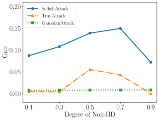
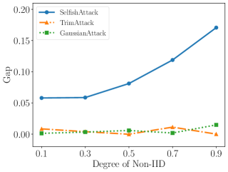
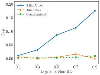
Impact of degree of Non-IID: Fig. 5 in Appendix shows the impact of degree of non-IID on SelfishAttack and compared attacks on CIFAR-10 dataset. We observe that our SelfishAttack consistently achieves much larger Gap than compared attacks when attacking different aggregation rules for different degrees of Non-IID. For instance, when attacking Median aggregation rule, our attack always achieves a Gap that is at least higher than the compared attacks, regardless of the degree of Non-IID. In particular, the compared attacks always have Gap close to 0 in most cases. One exception is that when using TrimAttack to attack the FedAvg aggregation rule and the degree of Non-IID is 0.5 or 0.7, the Gap is larger than 0.
Furthermore, our results demonstrate that as the degree of Non-IID increases, our SelfishAttack is more effective at increasing the Gap. There is only one exception: when attacking FedAvg, as the degree of Non-IID increases from to , our attack results in a lower Gap. This is due to the fact that when the degree of Non-IID is , there is a significant difference in the data distributions among the clients, leading to large differences between their local models. As a result, it becomes more challenging for the DFL system to obtain accurate local models through the FedAvg aggregation rule. Consequently, the local models of both selfish and non-selfish clients experience a performance drop. However, despite this, SelfishAttack still achieves a Gap of when attacking FedAvg and the degree of Non-IID is .
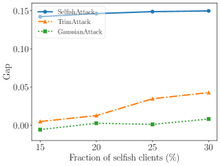
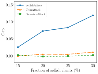
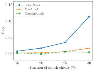
Impact of fraction of selfish clients: Fig. 6 in Appendix shows the impact of fraction of selfish clients on SelfishAttack and baseline attacks. We observe that SelfishAttack consistently outperforms compared attacks across different aggregation rules and various fraction of selfish clients. For instance, when attacking Median, the Gap under our attack is at least higher than the compared attacks if there are no less than of selfish clients. Moreover, except the case of attacking FedAvg with TrimAttack, where the Gap is larger than 0, the Gap obtained by the compared attacks is close to 0 in all other cases.
On the other hand, we find that under our attack, an increase in the number of selfish clients does not significantly affect Gap when the aggregation rule is FedAvg. However, when the aggregation rule is Median or Trimmed-mean, a larger fraction of selfish clients leads to a larger Gap. For example, when attacking Median, having 6 selfish clients ( selfish clients) results in a Gap that is approximately higher than the Gap achieved by 5 selfish clients ( selfish clients). We also observe that when attacking Median and Trimmed-mean, the larger number of selfish clients, the larger the upper bounds and the smaller the lower bounds described in Equations 9, 10, 14, and 15. This expands the range of attack for selfish clients, making the attack more effective.
| Aggregation Rule | FedAvg | Median | Trimmed-mean | ||||||
| MTAS | MTANS | Gap | MTAS | MTANS | Gap | MTAS | MTANS | Gap | |
| FedAvg | 0.475 | 0.326 | 0.150 | 0.478 | 0.326 | 0.152 | 0.470 | 0.326 | 0.144 |
| Median | 0.574 | 0.425 | 0.150 | 0.543 | 0.425 | 0.119 | 0.301 | 0.425 | -0.123 |
| Trimmed-mean | 0.597 | 0.484 | 0.113 | 0.596 | 0.484 | 0.113 | 0.597 | 0.484 | 0.113 |
| Aggregation Rule | MTAS | MTANS | Gap |
| Krum | 0.545 | 0.356 | 0.189 |
| FLTrust | 0.537 | 0.469 | 0.069 |
| FLDetector | 0.556 | 0.439 | 0.118 |
| FLAME | 0.525 | 0.420 | 0.105 |
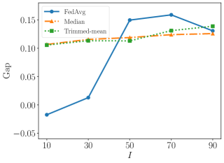
Impact of and : Figs. 7a and 7b in Appendix show the impact of and , respectively. The larger the and the smaller the , the earlier the selfish clients start to attack. We observe that our SelfishAttack is more sensitive to these two parameters when attacking FedAvg compared to Median and Trimmed-mean. From Fig. 7a, we observe that when does not exceed , our attack yields a low Gap, especially when the aggregation rule is FedAvg or Trimmed-mean, where the Gap is 0. In fact, in this case, the selfish clients do not start to attack until the end of the training process. When ranges from to , our attack exhibits relatively stable performance. When is and the aggregation rule is FedAvg, selfish clients initiate the attack before the local models have almost converged, resulting in a decline in the attack effectiveness. We also observe from Fig. 7b that when attacking Median and Trimmed-mean, the performance of SelfishAttack is almost not affected by , and the Gap obtained by our SelfishAttack is greater than in all cases. In contrast, when attacking FedAvg, the value of has a notable impact on Gap: when is not greater than , the Gap is close to 0; and when is not less than , the Gap is larger than .
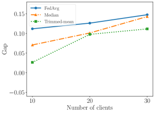
Impact of total number of clients: To explore the impact of the number of clients on SelfishAttack, we first divide the training data of CIFAR-10 dataset among clients, and then randomly select subsets of , , and clients from them while maintaining a fixed fraction of selfish clients at . Fig. 7c in Appendix shows the impact of the total number of clients on SelfishAttack. We observe that as the number of clients increases, our attack is more effective. For instance, when the aggregation rule is Median, increasing the number of clients from to results in a improvement in Gap. This may be because that although the fraction of selfish clients remains unchanged, the absolute number of selfish clients increases, thereby making the attack more effective.
Impact of aggregation rule used by selfish clients: Selfish clients can use different aggregation rules from non-selfish clients. Table 3 shows the results of our SelfishAttack when selfish and non-selfish clients use different aggregation rules. In Table 3, each column represents the aggregation rule used by selfish clients, and each row denotes the aggregation rule used by non-selfish clients. For each aggregation rule used by non-selfish clients, we apply the corresponding version of SelfishAttack. For instance, when the non-selfish clients use Trimmed-mean, the selfish clients craft their shared models based on Trimmed-mean aggregation rule. We observe that the Gap exceeds in most cases, with only one exception: when non-selfish clients use Median and selfish clients use Trimmed-mean, SelfishAttack results in a poor Gap. Overall, regardless of the aggregation rule employed by non-selfish clients, it is consistently a better choice for selfish clients to use the FedAvg aggregation rule.
Attacking other aggregation rules: Table 4 shows the results of our SelfishAttack when non-selfish clients use other aggregation rules (e.g., Krum, FLTrust, FLDetector, and FLAME), and selfish clients use FedAvg. Selfish clients craft their shared models using the FedAvg based version of SelfishAttack when the non-selfish clients use Krum, FLTrust, or FLDetector. We also tailor our attack to FLAME, and the details are shown in Appendix A.4. We observe that our SelfishAttack can transfer to these aggregation rules. Specifically, when attacking Krum, FLTrust, FLDetector, and FLAME, the corresponding Gaps obtained by our SelfishAttack exceed , , , and , respectively.
6 Discussion and Limitations
Combined attack strategies for selfish clients: Recall that the selfish clients have the flexibility to choose the shared models they send to non-selfish clients, the aggregation rule to use, and the subsets of received shared models used for aggregation. In our SelfishAttack, we mainly focus on the design of the shared models sent by selfish clients to non-selfish ones. In the experiments, we explored the impact of selfish clients using different aggregation rules and subsets of shared models for aggregation on the effectiveness of SelfishAttack. However, it is an interesting future work to explore how to combine the three strategies, i.e., shared model crafting, aggregation rule, and subset of shared models for aggregation, into a more effective combined strategy.
Defending against SelfishAttack: Byzantine-robust aggregation rules are defenses against “outlier” shared models, which can be applied to defend against SelfishAttack. However, we theoretically show that Median and Trimmed-mean cannot defend against our SelfishAttack, as the selfish clients can derive the optimal shared models to minimize a weighted sum of the two loss terms that quantify the two attack goals respectively. Moreover, we empirically show that other more advanced aggregation rules such as Krum, FLTrust, FLDetector, and FLAME cannot defend against SelfishAttack as well. It is an interesting future work to explore new defense mechanisms to defend against SelfishAttack. In SelfishAttack, a selfish client sends different shared models to different non-selfish clients. Therefore, one possible direction is to explore cryptographic techniques to enforce that a selfish client sends the same shared model to all clients. We expect such defense can reduce the attack effectiveness, though may not completely eliminate the attack since a selfish client can still send the same carefully crafted shared model to all non-selfish clients. Another direction for defense is to use trusted execution environment, e.g., NVIDIA H100 GPU. In particular, the local training and model sharing of each client is performed in a trusted execution environment, whose remote attestation capability enables a non-selfish client to verify that the shared models from other clients are genuine.
7 Conclusion and Future Work
In this paper, we propose SelfishAttack, the first competitive advantage attack to DFL. Using SelfishAttack, selfish clients can send carefully crafted shared models to non-selfish ones such that 1) selfish clients can still learn more accurate local models than performing DFL among themselves, and 2) selfish clients can learn much more accurate local models than non-selfish ones. We show that such shared models can be crafted by solving an optimization problem that aims to minimize a weighted sum of two loss terms quantifying the two attack goals respectively. Our evaluation on three benchmark datasets shows that SelfishAttack achieves the two attack goals and outperforms conventional poisoning attacks. Interesting future work includes 1) developing combined attack strategies, and 2) exploring new defenses against SelfishAttack.
References
- [1] Eugene Bagdasaryan, Andreas Veit, Yiqing Hua, Deborah Estrin, and Vitaly Shmatikov. How to backdoor federated learning. In AISTATS, 2020.
- [2] Arjun Nitin Bhagoji, Supriyo Chakraborty, Prateek Mittal, and Seraphin Calo. Analyzing federated learning through an adversarial lens. In ICML, 2019.
- [3] Peva Blanchard, El Mahdi El Mhamdi, Rachid Guerraoui, and Julien Stainer. Machine learning with adversaries: Byzantine tolerant gradient descent. In NeurIPS, 2017.
- [4] Peva Blanchard, El Mahdi El Mhamdi, Rachid Guerraoui, and Julien Stainer. Machine learning with adversaries: Byzantine tolerant gradient descent. In NIPS, 2017.
- [5] Sebastian Caldas, Sai Meher Karthik Duddu, Peter Wu, Tian Li, Jakub Konečnỳ, H Brendan McMahan, Virginia Smith, and Ameet Talwalkar. Leaf: A benchmark for federated settings. arXiv preprint arXiv:1812.01097, 2018.
- [6] Xiaoyu Cao, Minghong Fang, Jia Liu, and Neil Zhenqiang Gong. Fltrust: Byzantine-robust federated learning via trust bootstrapping. In NDSS, 2021.
- [7] Xiaoyu Cao and Neil Zhenqiang Gong. Mpaf: Model poisoning attacks to federated learning based on fake clients. In CVPR Workshops, 2022.
- [8] Rong Dai, Li Shen, Fengxiang He, Xinmei Tian, and Dacheng Tao. Dispfl: Towards communication-efficient personalized federated learning via decentralized sparse training. In ICML, 2022.
- [9] Cheng Fang, Zhixiong Yang, and Waheed U Bajwa. Bridge: Byzantine-resilient decentralized gradient descent. arXiv preprint arXiv:1908.08098, 2019.
- [10] Minghong Fang, Xiaoyu Cao, Jinyuan Jia, and Neil Gong. Local model poisoning attacks to byzantine-robust federated learning. In USENIX Security Symposium, 2020.
- [11] Alec Go, Richa Bhayani, and Lei Huang. Twitter sentiment classification using distant supervision. CS224N project report, Stanford, 2009.
- [12] Shangwei Guo, Tianwei Zhang, Han Yu, Xiaofei Xie, Lei Ma, Tao Xiang, and Yang Liu. Byzantine-resilient decentralized stochastic gradient descent. In IEEE Transactions on Circuits and Systems for Video Technology, 2021.
- [13] Sepp Hochreiter and Jürgen Schmidhuber. Long short-term memory. In Neural computation, 1997.
- [14] Alex Krizhevsky, Geoffrey Hinton, et al. Learning multiple layers of features from tiny images. 2009.
- [15] Leslie Lamport, Robert Shostak, and Marshall Pease. The byzantine generals problem. In Concurrency: the works of leslie lamport, 2019.
- [16] Yann LeCun, Corinna Cortes, and CJ Burges. Mnist handwritten digit database. Available: http://yann. lecun. com/exdb/mnist, 1998.
- [17] H Brendan McMahan, Eider Moore, Daniel Ramage, Seth Hampson, et al. Communication-efficient learning of deep networks from decentralized data. In AISTATS, 2017.
- [18] H. Brendan McMahan, Eider Moore, Daniel Ramage, Seth Hampson, and Blaise Agüera y Arcas. Communication-efficient learning of deep networks from decentralized data. In AISTATS, 2017.
- [19] Thien Duc Nguyen, Phillip Rieger, Roberta De Viti, Huili Chen, Björn B Brandenburg, Hossein Yalame, Helen Möllering, Hossein Fereidooni, Samuel Marchal, Markus Miettinen, et al. Flame: Taming backdoors in federated learning. In USENIX Security Symposium, 2022.
- [20] Jeffrey Pennington, Richard Socher, and Christopher D Manning. Glove: Global vectors for word representation. In EMNLP, 2014.
- [21] Zhaoxian Wu, Tianyi Chen, and Qing Ling. Byzantine-resilient decentralized stochastic optimization with robust aggregation rules. arXiv preprint arXiv:2206.04568, 2022.
- [22] Zhixiong Yang and Waheed U Bajwa. Byrdie: Byzantine-resilient distributed coordinate descent for decentralized learning. In IEEE Transactions on Signal and Information Processing over Networks, 2019.
- [23] Zhixiong Yang, Arpita Gang, and Waheed U Bajwa. Adversary-resilient distributed and decentralized statistical inference and machine learning: An overview of recent advances under the byzantine threat model. In IEEE Signal Processing Magazine, 2020.
- [24] Gokberk Yar, Cristina Nita-Rotaru, and Alina Oprea. Backdoor attacks in peer-to-peer federated learning. arXiv preprint arXiv:2301.09732, 2023.
- [25] Dong Yin, Yudong Chen, Ramchandran Kannan, and Peter Bartlett. Byzantine-robust distributed learning: Towards optimal statistical rates. In ICML, 2018.
- [26] Zaixi Zhang, Xiaoyu Cao, Jinyuan Jia, and Neil Zhenqiang Gong. Fldetector: Defending federated learning against model poisoning attacks via detecting malicious clients. In KDD, 2022.
Appendix A Appendix
A.1 Proof of Theorem 1
According to Equation 8, we have:
| (24) | ||||
A.2 Proof of Theorem 2
Case I: . We have
Thus
So ranks -th among , and rank -th,-th,respectively. We have
| (25) |
Case II: . We have
Thus
So ranks -th among , and rank -th and -th, respectively. Therefore,
| (26) |
Case III: . In this case, we can find such that and . Thus
rank among , respectively. Because and , the median value of must between and , which means . So we have
| (27) |
After summarizing results of Equations 25, 26, and 27, we have
A.3 Proof of Theorem 3
We discuss two cases based on the definitions of Equations 16-19 and Equations 20-23. Note that . Case I: . According to Equation 16, we need to find maximum , such that , and
| (28) |
Since , when , we have
| (29) | ||||
so such exists, and . If , there are no Part II selfish model parameters, and
Since , we have . Note that in this case all the shared model parameters of selfish clients are Part I model parameters, which are all less than , so
| (30) |
If , then we prove that when . In fact, the right side can be directly obtained by Equation 16, so we only need to prove the left side. Since is maximum, we have
| (31) |
So we have
| (32) | ||||
Thus for according to Equation 19. Hence, when calculating the trimmed mean value of , will be filtered out since they are the largest values in the -th dimension, and will be filtered out since they are the smallest values in the -th dimension, and
| (33) | ||||
Case II: . Similar to Case I, according to Equation 20, first we need to find minimum such that , and
| (34) |
Since , when , we have
| (35) | ||||
so such exists, and . If , there are no Part II selfish model parameters and we have
| (36) |
If , then we can similarly prove when . Hence, when calculating the trimmed mean value of , will be filtered out since they are the smallest values in the -th dimension, and will be filtered out since they are the largest values in the -th dimension, and
| (37) | ||||
After summarizing results of Equations 30, 33, 36, and 37, we have:
A.4 Attacking FLAME
Recall that FLAME first clusters models based on cosine distances between them and selects the largest cluster with no fewer than models. To encourage the clustering algorithm to misclassify as many non-selfish clients as possible as selfish and subsequently remove them, we select a subset of non-selfish clients. We then craft shared models of selfish clients such that the crafted models are close to the shared models of these selected non-selfish clients, while keeping them distinctly different from the models of the remaining non-selfish clients. Specifically, when client employs the FLAME aggregation rule, we first identify shared models of non-selfish clients with the smallest cosine distance to , denoted as . Then, we craft the shared model of selfish clients as follows:
| (38) | ||||
where and are some constants. In our experiments, we set and . In Equation 38, the first term aims to bring the crafted models closer to the selected shared models; the second term satisfies our utility goal, which is to maintain the proximity of client ’s post-aggregation local model to its pre-aggregation local model; and the third term pushes the crafted models away from the unselected models, which satisfies our competitive advantage goal. The selfish clients use the Median aggregation rule to aggregate received models from all clients.
| Notation | Description |
| Number of non-selfish clients. | |
| Number of selfish clients. | |
| Hyperparameter in our optimization problem. | |
| Pre-aggregation local model of client . | |
| -th dimension of . | |
| Post-aggregation local model of client . | |
| Optimal solution of our optimization problem. | |
| Model aggregated by non-selfish clients’ shared models. | |
| Upper bound of . | |
| Lower bound of . | |
| Shared model that client sends to client . | |
| Pre-aggregation local model of client at round . | |
| Post-aggregation local model of client at round . |
| Parameter | CIFAR-10 | FEMNIST | Sent140 |
| # clients | 20 | ||
| # selfish clients | 6 | ||
| # local training epochs | 3 | ||
| Learning rate | |||
| Optimizer | Adam (weight decay=) | ||
| # global training rounds | 600 | 600 | 1,000 |
| Batch size | 128 | 256 | 256 |
| Layer | Size |
| Input | |
| Convolution + ReLU | |
| Max Pooling | |
| Convolution + ReLU | |
| Max Pooling | |
| Fully Connected + ReLU | 100 |
| Fully Connected | 10 |
| Layer | Size |
| Input | |
| Convolution + ReLU | |
| Max Pooling | |
| Convolution + ReLU | |
| Max Pooling | |
| Fully Connected | 62 |
| Layer | Configuration | |||
| Embedding |
|
|||
| LSTM |
|
|||
| Fully Connected |
|
|||
| Fully Connected |
|