Perturbing the Stable Accretion Disk in Kerr and 4-D Einstein-Gauss-Bonnet Gravities: Comprehensive Analysis of Instabilities and Dynamics

Abstract

The study of a disturbed accretion disk holds great significance in the realm of astrophysics. This is because such events play a crucial role in revealing the nature of disk structure, the release of energy, and the generated shock waves. Thus, they can help explain the causes of $X-$ray emissions observed in black hole accretion disk systems. In this paper, we perturb the stable disk formed by spherical accretion around Kerr and EGB black holes. This perturbation reveals one- and two-armed spiral shock waves on the disk’s surface. We find a strong connection between these waves and the black hole’s spin parameter ($a/M$) and the EGB coupling constant ($\alpha$). Specifically, we found that as $\alpha$ increases in the negative direction, the dynamics of the disk and the waves become more chaotic. Additionally, we observe that the angular momentum of the perturbing matter significantly affects mass accretion and the oscillation of the arising shock waves. This allows us to observe changes in $QPOs$ frequencies. Particularly, perturbations with angular momentum matches the observed $C-$type $QPOs$ frequencies of $GRS1915+105$ source. Thus, we conclude that the possibility of the shock waves occurring within the vicinity of $GRS1915+105$ is substantial.

1 Introduction

The perturbations of accretion disks around the black holes have been conducted on vastly different scales, ranging from stellar-mass black holes in $X-$ray binaries to supermassive black holes in Active Galactic Nuclei (AGN). These investigations aim to understand the effects of various physical processes and interactions that may lead to perturbations in the accretion disks.

In $X-$ray binaries, where a stellar-mass black hole accreates matter from a companion star, observations have revealed fluctuations in the emitted radiation, broad emission lines, and Quasi-Periodic Oscillations (QPOs). These phenomena suggest the presence of perturbed accretion disks, which may be influenced by interactions with the companion star or other external sources. Several observed $X-$ray binaries have been identified as potential candidates with perturbed accretion disks. $GRS$ $1915+105$ was examined through observations of high-frequency QPOs and rapid flux variations (Feng et al., 2022; Ricketts et al., 2023). The intense radiation from $MAXI$ $J1820+070$ provided evidence of a perturbed accretion disk, possibly caused by instabilities or interactions with surrounding matter(Zhang et al., 2023). The findings from $GX$ $339-4$ were in line with the presence of a perturbed accretion disk (Jin et al., 2023) which shown variations in $X-$ray emission, spectral changes, and QPOs. The perturbation likely arise from interactions with the companion star or other sources of external perturbations. Cygnus $X-1$ has exhibited spectral variability and QPOs due to the perturbation of the accretion disk which could be influenced by interactions with a companion star or clumps of material in the disk (Miller et al., 2012; Dong et al., 2022). The presence of perturbations in the accretion disk, possibly caused by interactions with the companion star or transient structures in the disk could cause a strong $X-$ ray variability and complex flaring behavior.

Remillard & McClintock (2006) investigated the properties and behavior of $20$ $X-$ray binaries, with $17$ of them being transient systems confirmed to host a dynamically-active black hole. Over the past decade, these transient sources underwent intensive monitoring during their typical year-long outburst cycles, utilizing the large-area timing detector of the Rossi $X-$Ray Timing Explorer. The evolution of these sources exhibits complexity, but a comprehensive comparison of six selected systems reveals shared patterns in their behavior. Central to this comparison are three distinct $X-$ray states of accretion, meticulously examined and quantitatively defined. They explored various phenomena occurring in strong gravitational fields, such as relativistically-broadened $Fe$ lines, high-frequency QPOs (ranging from $100$ to $450$ $Hz$), and relativistic radio and $X-$ray jets. These observations shed light on the interactions between black holes and their surrounding environments, providing valuable insights that complement the knowledge gained from gravitational wave detectors.

AGN consist of supermassive black holes (SMBHs) with masses ranging from $10^{6}M_{\odot}$ to $10^{10}M_{\odot}$, located at the center of a galaxies. These black holes continuously accreate matter, leading to their highly luminous nature. The presence of such SMBHs in galaxies suggests that supermassive black hole binaries (SMBHs) should be common in galactic nuclei (Khan et al., 2016). However, detecting these systems in close proximity to the central object is extremely challenging (D’Orazio & Loeb, 2018). In the era of multi-messenger astrophysics, understanding the significance of SMBHs in close proximity to the central object goes beyond evolutionary processes. They are regarded as crucial targets for connecting gravitational wave detections with electromagnetic counterparts (Bowen et al., 2019). This possibility is promising since merging black holes could interact with the surrounding gas, potentially leading to electromagnetic counterparts (Palenzuela et al., 2010).

$J095036+512838$ is classified as an AGN. It was investigated using observations of $Ly-$alpha and $C$ $IV$ broad lines (Runnoe et al., 2021; Mohammed et al., 2023). It belongs to a category of galaxies characterized by an extraordinarily bright center, believed to be fueled by a supermassive black hole that attracts and absorbs surrounding matter. The remarkable luminosity of AGNs is attributed to the intense radiation emanating from the accretion disk encircling the central black hole.

Perturbation is an immensely significant physical phenomenon with the potential to provide valuable insights into the origin of $X-$ray emissions and QPOs observed in the aforementioned astrophysical systems (Ingram & Motta, 2019; Rana & Mangalam, 2020). The perturbation induces disturbances in the accretion disk, breaking its spherical symmetry and generating strong shock waves that may oscillate during the system’s evolution, even after reaching a steady state. As a consequence of these disturbances or irregularities, the observed emission lines experience shifts from their expected positions. These shifts offer valuable insights into the properties of the accretion disk, the environment surrounding the supermassive black hole, and the physical processes taking place in its vicinity. Analyzing these shifts aids astrophysicists in understanding the dynamics and characteristics of the black hole systems.

Numerical investigation of the accretion disk helps us comprehend the structure, instabilities, and the occurrence of quasi-periodic behavior near the black hole for different gravities. This deeper understanding contributes to unraveling the underlying physical mechanisms responsible for the observed $X-$ray frequencies and variations (Chakrabarti et al., 2002). Dönmez (2006) investigates the dynamic evolution of star-disk interaction in the vicinity of a massive black hole, where physical perturbation plays a dominant role over other processes, and the gravitational region exhibits strong effects. A numerical simulation is employed to model the accretion disk around the black hole when a star gets captured by it. When the accretion disk, whether in a steady state or not, undergoes perturbation due to the presence of the star, the interaction results in the destruction of the disk surrounding the black hole. The destruction of the accretion disk gives rise to a spiral shock wave, leading to the loss of angular momentum. Stone & Pringle (2001) conducted a comprehensive exploration of the vertical shear instability (VSI) in accretion disks using 3D numerical simulations. The VSI is a hydrodynamic instability that arises from vertical velocity shear within the accretion disk. The study delves into the growth and characteristics of the VSI in various regions of the disk, shedding light on its influence on the overall dynamics of the disk. Notably, the simulations show that the VSI can induce substantial turbulence and vertical mixing, potentially impacting the accretion process and angular momentum transport within the disk.

In this study, we investigate dynamics of the perturbed accretion disks using a numerical relativistic hydrodynamics code, which allows us to gain valuable insights into the behavior and characteristics of these disks in the presence of strong gravitational fields, particularly in the vicinity of Kerr and Einstein-Gauss-Bonnet (EGB) black holes. Our numerical simulations focus on modeling the dynamics of accretion disks under perturbations arising from interactions with companion objects. The results from our numerical simulations reveal that perturbations in accretion disks can give rise to the formation of shock waves, oscillations, and other complex phenomena. The generation of shock waves leads to the heating of matter within the accretion disk, resulting in the production of electromagnetic radiation. As a result, the perturbation induces shock waves, which, in turn, impact various aspects of the system, such as the light curve, radiation spectrum (including $QPOs$), and outburst durations (Zhilkin & Bisikalo, 2021). The physical origins of QPO frequencies are not yet fully understood (Ingram & Motta, 2019). In this work, we explain some observed QPOs with tbe shock waves generated by perturbing a stable disk. We also examine the influence of various parameters, including the black hole’s spin ($a/M$), the strength of the perturbation, and the EGB coupling constant ($\alpha$), on the behavior of the disk. Through these simulations, we aim to shed light on the intricate interplay between the accretion disk and external perturbations, providing a better understanding of the physical processes occurring in these extreme gravitational environments. The findings contribute to our broader comprehension of accretion processes in the vicinity of the black holes and their significance in astrophysical observations.

The structure of the rest of the paper is outlined as follows. In Section 2, we introduce the Kerr and 4D EGB black hole spacetime metrics, along with lapse functions and shift vectors. The equations for general relativistic hydrodynamics are presented in a conserved form suitable for high-resolution shock capturing schemes. Section 3 presents the initial conditions for the setup of the steady-state accretion disk and perturbations. The necessary boundary conditions to yield physical solutions are also defined in this same section. To place numerical computations on a stronger scientific foundation, the astrophysical applications of numerical results are important. Section 4 includes $X-$ray binary systems and AGN sources, which are thought to have perturbed disks observationally. In Section 5, we conduct a numerical examination of the initial steady-state accretion disk, the structure and instabilities of the disk around Kerr and EGB black holes, as well as QPO frequencies that can serve as a comparison basis for various sources. The impact of using alternative gravity on the structure and instability of the perturbed accretion disk has been discussed. Finally, in Section 6 we discuss and summarize the numerical results, and potential future research directions are provided. We use geometrized units with $c=G=1$ throughout the paper to simplify the equations.

2 Governing Equations

2.1 Metrics for Kerr and Einstein-Gauss-Bonnet gravities

Using different gravities, such as those in Kerr and 4-D EGB black holes, allows for modeling the behavior of the accretion disk in the strong gravitational field near black holes. This approach provides a more comprehensive understanding of the disk’s dynamics, including shock wave formation, oscillations, and other complex behaviors. By comparing the numerical results obtained with various gravity models, researchers can gain new insights into the underlying physical processes, enhance their understanding of the black hole-disk systems, and bridge theoretical and observational approaches.

The Kerr black hole in Boyer-Lindquist coordinates is described by the following metric (Dönmez et al., 2011):

$$ds^{2}=-\left(1-\frac{2Mr}{\sum^{2}}\right)dt^{2}-\frac{4Mra}{\sum^{2}}sin^{2}\theta dtd\phi+\frac{\sum^{2}}{\Delta_{1}}dr^{2}+\sum^{2}d\theta^{2}+\frac{A}{\sum^{2}}sin^{2}\theta d\phi^{2}$$ (1)

where $\Delta_{1}=r^{2}-2Mr+a^{2}$, and $A=(r^{2}+a^{2})^{2}-a^{2}\Delta sin^{2}\theta$. In Boyer-Lindquist coordinates, the shift vector and lapse function of the Kerr metric are $\beta^{i}=(0,0,-2Mar/A)$ and $\tilde{\alpha}=(\sum^{2}\Delta_{1}/A)^{1/2}$.

Near the Kerr black hole, the strong gravitational field causes spacetime to curve significantly, leading to the alteration of the physical characteristics of the geometry in its vicinity. This curvature is a consequence of the black hole’s mass and angular momentum, and it results in intriguing phenomena such as frame-dragging, time dilation, and the existence of an event horizon.

$4D$ EGB gravity characterizes the curvature and physical properties of the spacetime in the vicinity of the rotating black hole, taking into account the gravitational effects predicted by the Einstein-Gauss-Bonnet theory. The $4D$ EGB rotating black hole metric is (Donmez, 2022; Donmez et al., 2022),

$$ds^{2} = -\frac{\Delta_{2}-a^{2}sin^{2}\theta}{\Sigma}dt^{2}+\frac{\Sigma}{\Delta_{2}}dr^{2}-2asin^{2}\theta\left(1-\frac{\Delta_{2}-a^{2}sin^{2}\theta}{\Sigma}\right)dtd\phi+\Sigma d\theta^{2}+$$ (2)

$$sin^{2}\theta\left[\Sigma+a^{2}sin^{2}\theta\left(2-\frac{\Delta_{2}-a^{2}sin^{2}\theta}{\Sigma}\right)\right]d\phi^{2}.$$

The expressions for $\Sigma$ and $\Delta_{2}$ are given by $\Sigma=r^{2}+a^{2}\cos^{2}\theta$ and $\Delta_{2}=r^{2}+a^{2}+\frac{r^{4}}{2\alpha}\left(1-\sqrt{1+\frac{8\alpha M}{r^{3}}}\right)$, respectively. Here, $a$, $\alpha$, and $M$ represent the black hole spin parameter, Gauss-Bonnet coupling constant, and mass of the black hole, respectively. The black hole horizon is determined by solving the equations $\Delta_{1}=0$ and $\Delta_{2}=0$. The lapse function $\tilde{\alpha}$ and the shift vectors of the $4D$ EGB metric are given as $\tilde{\alpha}=\sqrt{\frac{a^{2}(1-f(r))^{2}}{r^{2}+a^{2}(2-f(r))}+f(r)}$ and $\beta^{i}=\left(0,\frac{ar^{2}}{2\pi\alpha}\left(1-\sqrt{1+\frac{8\pi\alpha M}{r^{3}}}\right),0\right)$, respectively. Here, $f(r)=1+\frac{r^{2}}{2\alpha}\left(1-\sqrt{1+\frac{8\alpha M}{r^{3}}}\right)$. The EGB black hole is a modified theory of gravity that generalizes the traditional black hole solutions, such as the Schwarzschild and Kerr solutions, by incorporating an additional term involving the Gauss-Bonnet curvature. This extra term introduces higher curvature corrections, offering a new perspective on the behavior of the black holes in extreme conditions and higher-dimensional spacetime (Fernandes et al., 2022).

2.2 General Relativistic Equations

In the context of the perturbed accretion disk phenomenon, a fluid, which could be gas or dust originating from a companion star, undergoes gravitational attraction towards a massive object, such as a black hole, and subsequently perturbed the stable accretion disk. This process holds significance in gaining insights into the interaction between matter and black holes, as well as stable accretion disks. To investigate the perturbation of the disk process involving a perfect fluid, we explore the presence of rotating black holes, specifically the Kerr and EGB black holes, by solving the GRH equations in the curved background. The stress-energy-momentum tensor of the perfect fluid is taken into account to analyze the dynamical behavior and characteristics of the perturbed accretion disk in the vicinity of the rotating black holes.

$$T^{ab}=\rho hu^{a}u^{b}+Pg^{ab},$$ (3)

where $\rho$ representing the rest-mass density, $p$ denoting the fluid pressure, $h$ indicating the specific enthalpy, $u^{a}$ representing the $4$-velocity of the fluid, and $g^{ab}$ as the metric of the curved space-time. The indices $a$, $b$, and $c$ range from $0$ to $3$. To facilitate a comprehensive comparison of the dynamic evolution of the accretion disk around the rotating black hole, we utilize two distinct coordinate systems. The first involves the Kerr black hole in Boyer-Lindquist coordinates, while the second employs the rotating black hole metric in $4D$ EGB gravity as described in section 2.1.

In order to perform numerical solutions for the GRH equations, it is essential to transform them into a conserved form (Dönmez, 2004). By employing advanced numerical methods, the simulations of fluid dynamics in strong gravitational fields, such as those near spinning black holes, become more reliable and efficient, ensuring precise and trustworthy results.

$$\frac{\partial U}{\partial t}+\frac{\partial F^{r}}{\partial r}+\frac{\partial F^{\phi}}{\partial\phi}=S.$$ (4)

The conserved variables are denoted by the vectors $U$, $F^{r}$, $F^{\phi}$, and $S$, representing the conserved quantities, fluxes along the $r$ and $\phi$ directions, and sources, respectively. These conserved quantities are formulated in relation to the primitive variables, as shown below:

$$U=\begin{pmatrix}D\\ S_{j}\\ \tau\end{pmatrix}=\begin{pmatrix}\sqrt{\gamma}W\rho\\ \sqrt{\gamma}h\rho W^{2}v_{j}\\ \sqrt{\gamma}(h\rho W^{2}-P-W\rho)\end{pmatrix}.$$ (5)

In the given equation, the terms are defined as follows: the Lorentz factor is represented by $W=(1-\gamma_{a,b}v^{i}v^{j})^{1/2}$. The enthalpy is denoted by $h=1+\epsilon+P/\rho$, where $\epsilon$ stands for the internal energy. The three-velocity of the fluid is given by $v^{i}=u^{i}/W+\beta^{i}$. The pressure of the fluid is determined using the ideal gas equation of state, $P=(\Gamma-1)\rho\epsilon$. The three-metric is denoted as $\gamma_{i,j}$, and its determinant is $\gamma$, both calculated using the four-metric of the rotating black holes. Latin indices $i$ and $j$ range from $1$ to $3$. The flux and source terms can be computed for any metric using the following equations,

$$\vec{F}^{i}=\begin{pmatrix}\tilde{\alpha}\left(v^{i}-\frac{1}{\tilde{\alpha}\beta^{i}}\right)D\\ \tilde{\alpha}\left(\left(v^{i}-\frac{1}{\tilde{\alpha}\beta^{i}}\right)S_{j}+\sqrt{\gamma}P\delta^{i}_{j}\right)\\ \tilde{\alpha}\left(\left(v^{i}-\frac{1}{\tilde{\alpha}\beta^{i}}\right)\tau+\sqrt{\gamma}Pv^{i}\right)\end{pmatrix},$$ (6)

and,

$$\vec{S}=\begin{pmatrix}0\\ \tilde{\alpha}\sqrt{\gamma}T^{ab}g_{bc}\Gamma^{c}_{aj}\\ \tilde{\alpha}\sqrt{\gamma}\left(T^{a0}\partial_{a}\tilde{\alpha}-\tilde{\alpha}T^{ab}\Gamma^{0}_{ab}\right)\end{pmatrix},$$ (7)

where $\Gamma^{c}_{ab}$ is the Christoffel symbol.

3 Initial and Boundary Conditions

To examine the perturbed accretion disk surrounding the rotating Gauss-Bonnet black hole and make a comparison with the Kerr black hole, the General Relativistic Hydrodynamical (GRH) equations are solved on the equatorial plane. The simulation is performed using the code described in previous works by Dönmez (2004, 2012); Donmez (2006). The pressure of the accreated matter is calculated using the standard $\Gamma$ law equation of state for a perfect fluid, which is given by $P=(\Gamma-1)\rho\epsilon$, where $\Gamma=4/3$. Here, $P$ represents the pressure, $\rho$ is the density of the fluid, and $\epsilon$ denotes the internal energy.

To conduct the numerical simulation, two distinct initial conditions are utilized. Initially, the initial conditions presented in Donmez (2023) are employed to establish a stable and steady-state accretion disk around the black hole under spherical accretion conditions. The initial density and pressure profiles are carefully tuned to ensure that the speed of sound is equal to $C_{s}=0.1$ at the outer boundary of the computational domain. This adjustment is crucial to maintain appropriate conditions for the simulation and prevent unphysical behaviors at the boundaries. In pursuit of this goal, a constant density value ($\rho=10^{-4}$) is assigned, and the pressure is computed using the perfect fluid equation of state throughout the entire computational domain. This approach ensures uniform conditions and accurate representation of the fluid’s behavior across the simulation domain. Subsequently, numerical simulations are conducted on the equatorial plane, where gas is injected from the outer boundary with velocities $V^{r}=-0.01$, $V^{\phi}=0$, and density $\rho=1$. As seen in Donmez (2023), the disk reaches a steady-state at approximately $t=5000M$. However, to ensure certainty, the first phase is run up to $t=6000M$.

In the second stage of the modeling, the perturbation of the accretion disk is achieved by the infall of matter originating from a disrupting star or other physical mechanisms, causing it to fall toward the black hole from the outer boundary of the stable accretion disk that has reached a steady state. Once more, the initial density and pressure profiles are meticulously adjusted to ensure that the speed of sound equals $C_{s}=0.1$ at the outer boundary of the computational domain. This meticulous tuning guarantees appropriate conditions for the simulation, particularly at the domain’s outer limits. In order to introduce a physically acceptable perturbation, the numerical simulations are performed on the equatorial plane, with gas being injected from the outer boundary with velocities $V^{r}=-0.01$, $V^{\phi}=V_{\infty}\sqrt{\gamma^{\phi\phi}}sin\phi$, and density $\rho=2$ for $0<\phi<0.4$ at the outer boundary. $V_{\infty}$ is the asymptotic velocity of the matter at the outer boundary of the computational domain and it is given in Table 1. This setup ensures the infalling of the gas toward to the black hole supersonically, the generation of a significant perturbation in the system, allowing for a more insightful analysis of its behavior and dynamics. The detailed descriptions and a more comprehensive understanding of the initial models for rotating black holes, including both Kerr and Gauss-Bonnet black holes, can be found in Table 1.

Table 1: Adopted initial model used in the numerical simulation for Kerr and Gauss-Bonnet black holes. $Model$ is the name of the model. $type$ is the black hole types used in numerical simulations. $\alpha$ is Gauss-Bonnet coupling constant, and $a/M$ is the black hole rotation parameter. $nt/nt_{Kerr}$ is the ratio of the time steps required to reach to the maximum time $30000M$ to the time steps required for Kerr.

$Model$	$type$	$\alpha(M^{2})$	$a/M$	$V_{\infty}$	$nt/nt_{Kerr}$
$K028$		$-$	$0.28$	0.2	1
$K09$		$-$	$0.9$	0.2	1
$K028\_EGB1$		$-4.93$	$0.28$	0.2	1.15061
$K028\_EGB2$		$-3.03$	$0.28$	0.2	1.03582
$K028\_EGB3$	$Gauss-Bonnet$	$-0.37$	$0.28$	0.2	1.01832
$K028\_EGB4$		$0.096$	$0.28$	0.2	1.01561
$K028\_EGB5$		$0.41$	$0.28$	0.2	1.01375
$K028\_EGB6$		$0.68$	$0.28$	0.2	1.01163
$K09\_EGB1$		$-3.61$	$0.9$	0.2	1.15832
$K09\_EGB2$		$-1.56$	$0.9$	0.2	1.11819
$K09\_EGB3$		$-0.98$	$0.9$	0.2	1.11321
$K09\_EGB4$		$-0.443$	$0.9$	0.2	1.10711
$K09\_EGB5$	$Gauss-Bonnet$	$-0.063$	$0.9$	0.2	1.10408
$K09\_EGB6$		$-0.023$	$0.9$	0.2	1.10301
$K09\_EGB7$		$0.000625$	$0.9$	0.2	1.10337
$K09\_EGB8$		$0.05$	$0.9$	0.2	1.10313
$K09\_EGB9$		$0.05$	$0.9$	0	1.05249

Uniformly spaced zones are utilized to discretize the computational domain in both the radial and angular directions. In detail, there are $N_{r}=1024$ zones in the radial direction and $N_{\phi}=256$ zones in the angular direction. In the radial direction, the inner and outer boundaries of the computational domain are located at $r_{min}=3.7M$ and $r_{max}=100M$, respectively. The angular boundaries are specified as $\phi_{min}=0$ and $\phi_{max}=2\pi$. The code execution time, with $t_{max}=33000M$, is considerably longer than the expected time. Numerical verification has confirmed that the qualitative outcomes of the simulations, such as the presence of quasi-periodic oscillations (QPOs) and instabilities, the location of shocks, and the behavior of the accretion rates, are mostly independent of variations in the grid resolution (Donmez, Orhan, 2021; Donmez, 2022; Donmez et al., 2022). Furthermore, it is believed that positioning the outer boundary far enough away from the region where artifacts possibly produced at the outer boundary do not impact the physical solution.

Ensuring accurate boundary treatment is crucial to prevent the emergence of unphysical solutions in numerical simulations. To address this, specific boundary conditions are implemented for different regions: Inner Radial Boundary: An outflow boundary condition is applied to the inner radial boundary. This allows gas to flow into the black hole, employing a simple zeroth-order extrapolation technique. Outer Boundary: At the outer boundary, gas is continuously injected with initial velocities and density, as mentioned above, to account for the inflow of material until disk reached to steady state. Angular Direction $\phi$: Periodic boundary conditions are employed along the angular direction. This means that the fluid properties at one end of the domain are considered to be equivalent to the properties at the opposite end. By implementing these appropriate boundary conditions, the simulation aims to maintain the accuracy and reliability of the results, ensuring that unphysical artifacts are minimized or avoided.

4 Astrophysical Motivation

Observational evidence strongly suggests that accretion disks and electromagnetic radiations are closely related each other and that disks act as the driver for the radiation. There is a large, rich literature on the topic of astrophysical electromagnetic radiation and disks. The presence of perturbed disks has been observed in various astrophysical observations. These observations have revealed the existence of nonlinear physical mechanisms that can occur on the disk. For example, frequency fluctuations in the radiation observed in AGNs have been observed (Vaughan et al., 2011; McHardy, 2010; Gaskell & Goosmann, 2013). The reason for this is entirely due to perturbations caused by interactions with other stars around the accretion disk. On the other hand, while the black holes have a stable disk around them, they can be perturbed by the matter coming from surrounding stars, resulting in the formation of QPOs (Artymowicz & Lubow, 1996; Nixon et al., 2011). These are the consequences of the disk’s instability.

Observations from various sources have provided evidence that a substantial number of systems exhibit observed emission originating from perturbed accretion disks. For instance, $SMBH$ $J095036+512838$ was studied through observations of $Ly-$alpha and $C$ $IV$ broad lines (Runnoe et al., 2021; Mohammed et al., 2023). Similarly, $GRS$ $1915+105$ was examined through observations of high-frequency QPOs (Feng et al., 2022; Ricketts et al., 2023; Dhaka et al., 2023). The results from $GX$ $339-4$ are found to be consistent with the presence of a perturbed accretion disk (Jin et al., 2023). Additionally, the bright radiation from $MAXI$ $J1820+070$ indicated the presence of a perturbed accretion disk (Zhang et al., 2023). For the sources $MAXI$ $J1820+070$ and $MAXI$ $J1535-571$, Ding et al. (2023) observed cross and hypotenuse patterns, suggesting the presence of QPOs. It is plausible that these different types of QPOs could arise from similar underlying mechanisms.

Another observed system believed to originate from a perturbed accretion disk is $Mrk$ $1018$. $Mrk$ $1018$ is situated within a host galaxy that is currently experiencing a significant merger event. This particular galaxy is among the earliest identified Changing-Look (CL) AGNs, making a transition from a Seyfert $1.9$ to a Seyfert $1$ nucleus (Brogan et al., 2023). Over a span of $40$ years, the spectral type of $Mrk$ $1018$ underwent changes from Type $1.9$ to Type $1$, and subsequently reverted back to Type $1.9$. By analyzing archival spectral and imaging data, Kim et al. (2018) identified two kinematically distinct broad-line components, namely blueshifted and redshifted components. The velocity offset curve of the broad line displayed a characteristic pattern over time. Perturbations in the accretion disk caused by pericentric passages are deemed plausible in explaining the AGN activity and spectral change in $Mrk$ $1018$.

Specific low-frequency $QPOs$ originate from the geometric structure of the disk (Ingram & Motta, 2019) during the black hole-disk interaction. Here, we modeled the structure of the disk around the rotating black holes with different gravities, revealing how the disk’s structure and the resulting shock waves depend on the black hole’s spin parameter and EGB coupling constant. This allowes us to explore the potential physical mechanisms behind the observed low-frequency $QPOs$, which we will further elaborate on in the following sections.

5 The Numerical Simulation of the accretion toward 4D EGB Rotating and Kerr Black Holes

This section presents results from our numerical simulation exploring the dynamics of the accretion disk around a black hole, following the perturbation of the steady-state disk by a donor star in the $X-$ray binary system. We have uncovered the instabilities, the dynamics of spiral shock waves, and potential QPOs on the disk, which manifest after the disk attains a quasi-equilibrium state.

5.1 Formation of Initial Steady-State Accretion Disk

In astrophysical systems, in order to observe regular emissions, it is necessary to reveal that a regular physical mechanism is formed on the disk. To reveal this, in this article, we are examining the instabilities caused by the perturbation of the disk. In order to perturb the disk effectively, we need to analytically utilize disks in our simulation that have been formed around the black hole through various physical mechanisms. For example, because it is known analytically in Schwarzschild and Kerr gravity around the black holes, we studied the perturbation of these tori in our previous study (Dönmez, 2014). The analytic solutions of tori around the non-rotating and rotating black holes are not known in EGB gravity. For these reasons and to be able to perturb a different stable disk, we perturbed the stable disks we found in our previous study (Donmez, 2023).

The initial stable disk was formed as a result of the matter scattered around after a supernova explosion and falling back onto the newly formed black hole. This situation is both explained in Section.3 and can be seen in detail in (Donmez, 2023) regarding the stability status of the formation disk. In Fig.1, the logarithmic colored density of the disk that has reached a steady-state for a model used in (Donmez, 2023) is given, seen in left panel. In the right panel of Fig.1, the stability behavior, which varies over time, is derived from the calculation of the mass accretion rate at the inner boundary at the point of the disk closest the black hole. Especially, the graph on the right one shows that the disk reached a steady-state around $t=5000M$ and always maintained its stable structure. And it has been explained again in Section.5 in (Donmez, 2023) that the disk do not oscillate after reaching a steady-state. The solid circle shown in the right panel of Fig.1 represents the point in time when the disk experiences perturbation, following a certain period after it has achieved stability. This circumstance will be elaborated further in the subsequent sections.

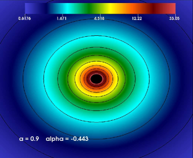
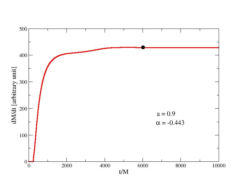
Figure 1: The logarithmic rest-mass density observed at t = 6000M and the mass accretion rate plotted as a function of time, demonstrating how this rate evolves over the simulated period. The both plots depict the formation of an initial steady-state accretion disk.

5.2 The Perturbed Accretion Disk around the Rotating EGB Black Hole

Modeling a perturbed stable accretion disk are crucial to understanding the behavior of matter around black holes, determining the mass accretion rate towards the black hole, unveiling the physical mechanism of shock waves formed on the disk (Aoki et al., 2004), variation of the disk’s light emission, and consequently explaining the observed QPOs (Abramowicz & Fragile, 2013). Here, it is shown how the stable disk around the rotating black holes, as presented in section 5.1, responds to perturbation when perturbed. The changes in the shock wave resulting from the perturbation are illustrated, and how these changes depend on the parameters is demonstrated.

Figures 2 and 3 illustrate how the mass density of the stable disk changing over time either right before being perturbed or right after being perturbed. These snapshots are selected to correspond to the same time steps between $t=5000M$ and $t=30000M$ for each model. The steady-state disk is perturbed at $t=6000M$ in all models. As seen in the figures, the disk responds to the perturbation, and initially, a significant change in the dynamic structure of the disk is observed. These changes continue for a while, and then the disk reaches a steady-state. It is observed that a shock wave formed on the disk at around $t=18000M$. This shock wave initially oscillates but at approximately $t=21000M$, it undergoes a quasi-periodic oscillation. This phenomenon is observed throughout the entire simulation process. During the time from the initial perturbation of the disk until it reaches a steady-state, it is observed that matter fall into the black hole. Simultaneously, the regularly fed disk initially creates a one-armed and then a two-armed shock waves. These arms appear to be mechanisms regularly feeding the black hole.

Figure 2 illustrates the behavior of the accretion disk around a rapidly rotating black hole with a spin parameter $a/M=0.9$ under different gravities (Kerr and EGB), while Fig.3 demonstrates the dynamics of a perturbed disk around a slowly rotating black hole with a spin parameter $a/M=0.28$ under various gravities. In both figures, the first rows depict changes in the dynamics of the disk around the Kerr black hole, while the second and third rows illustrate how these disks respond to perturbations in EGB gravity for the positive and negative maximum values of $\alpha$. Overall, the disk’s response to perturbations exhibits similar dynamic structures and shock wave formation in all models, but there are significant differences observed in the strength of oscillations, the amount of matter accreating onto the black hole, and the time it takes for these phenomena to occur. These differences lead to variations in the physical characteristics of the QPOs. As clearly seen in the figures, the times corresponding to the same time steps are shorter in EGB gravity compared to Kerr. This indicates that the disk structure and formation in EGB exhibit a more chaotic behavior. Additionally, the growth of $\alpha$ in the negative direction significantly increases the intensity of chaotic behavior.

Finally, when comparing Figs.2 and 3, it can be observed that the rotation parameter of the black hole affects the shock cone of flow originating from the disk and its impact on oscillations. Especially in regions with strong gravity, such as near to the black hole horizon, it has been observed that a rapidly rotating black hole curves the space-time, and causing the shock cone attached to the surface to bend. This is particularly significant in the strong gravity region. It causes the more matter falling into the black hole and the resulting QPOs.

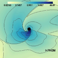
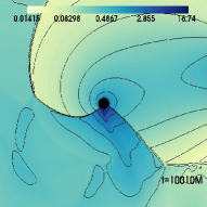
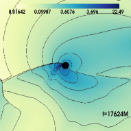
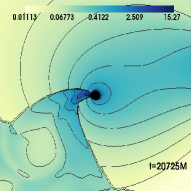
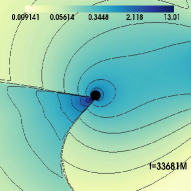
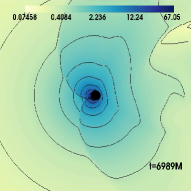
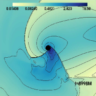
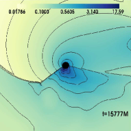
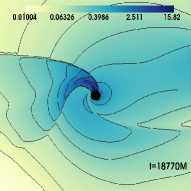
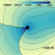
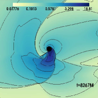
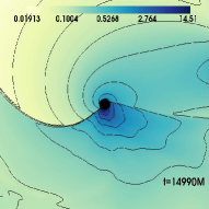
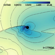
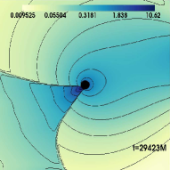
Figure 2: Snapshots of the logarithmic rest-mass density are provided at different times for different values of EGB coupling constant $\alpha$ for $a/M=0.9$. The first row shows how the dynamic structure of the accretion disk around the Kerr black hole changes over time during the perturbation process (model K09). The second row illustrates the dynamic changes in the disk for the largest $\alpha$ value used in Table 1 with $a/M=0.9$ (model K09_EGB8), and the third row displays the dynamic changes in the disk corresponding to the largest value for negative $\alpha$ (model K09_EGB1). In each column here, the dynamic structure of the disk at times corresponding to the same time steps for different models is displayed. Thus, it reveals the chaotic nature of the disk’s dynamic structure. The dynamic boundary marked here extends from $[x,y]$ to $[-70M,70M]$.

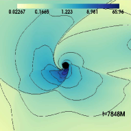
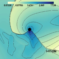
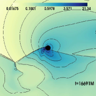
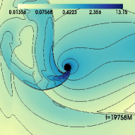
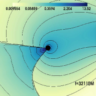
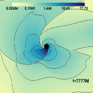
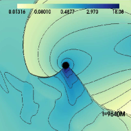
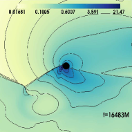
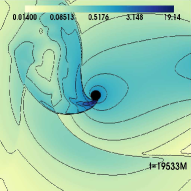
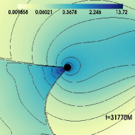
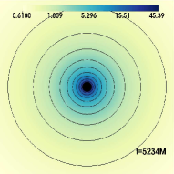
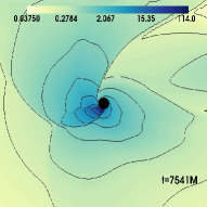
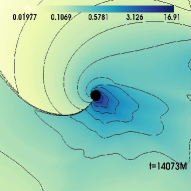
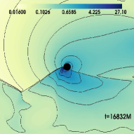
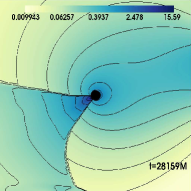
Figure 3: Same as Fig.2 but it is for $a/M=0.28$. They have been obtained using models $K028$, $K028\_EGB6$, and $K028\_EGB1$.

As a result of the interaction between the black hole and the disk, matter falls towards the black hole under the effect of gravitational force. The rate at which this falling matter is observed per unit time is known as the mass accretion rate. Mass accretion is generally observed at a point close to the black hole, more precisely at the boundary of the disk next to the black hole. In this way, many features of the disk are revealed. Because the mass accretion rate reveals whether the disk oscillates over time, the amount of increase in the mass of the black hole, the frequency and thus the energy of the electromagnetic radiation in the region where there is high gravitational pull, and the causes of jet formation around the black hole. Therefore, calculating the mass accretion rate is necessary to reveal some of the features mentioned above. The general relativistic mass accretion rate on the equatorial plane is calculated with the following equation(Petrich et al., 1989; Dönmez et al., 2011),

$$\frac{dM}{dt}=\int_{0}^{2\pi}\alpha\sqrt{\gamma}D\left(v^{r}-\frac{\beta^{r}}{\alpha}\right)d\phi$$ (8)

.

The mass accretion rate not only provides information about the behavior of the disk structure but can also be used to reveal the physical properties of the electromagnetic radiation that may arise close to the black hole horizon as a result of the black hole-disk interactions. Here we compute the mass accretion rate around the black hole at $r=3.88M$ very close to the black hole horizon, $r=3.7M$. Because the inner part of the disk, which is close to the black hole horizon and has a strong gravity, generates QPO modes (Ingram & Motta, 2019; Motta & Belloni, 2023). This way, we can compare the numerical results with observations.

In Fig.4, the mass accretion rate is shown for the $a/M=0.28$ and $a/M=0.9$ cases, illustrating how it changes over time in Kerr and EGB gravities. It is observed that as the initial stable accretion disk formation occurs, the mass accretion rate exponentially increases over time and reaching a steady-state around $t=4500M$. In the steady-state at $t=6000M$, the disk is perturbed. It is important to note that the same perturbation parameters are applied to all models depicted in Fig.4. The perturbed disk rapidly loses mass (with most of the material falling into the black hole, while some is dragged beyond the computational domain). Around $t=7300M$, mass accretion rate has started exhibiting the non-linear oscillations around a specific value ($dM/dt\sim 30$). After undergoing strong oscillations until approximately $t=19500M$, it reached a quasi-periodic phase with $dM/dt\sim 20$. In other words, the disk around the black hole has reached a steady-state and maintained this phase throughout the simulation time ($t=32000M$). As seen in the highlighted graphic within Fig.4, the effect of the EGB coupling constant, $\alpha$, significantly impacts the dynamic structure of the disk and the accreated more matter during the stable disk formation process in the case of a smaller black hole spin parameter, $a/M=0.28$. After perturbation, shock waves occur on the disk, and the disk returns to a steady-state. In this scenario, the effect of $\alpha$ is more pronounced in the case of $a/M=0.9$, suggesting that $\alpha$ has a greater influence on mass accretion and oscillations within the disk when shock waves are present. It has been observed that as the value of $\alpha$ increases, the mass accretion rate also increases which in turn causes an increase in the density of the accretion accretion disk as seen in Fig.5. This finding has been also confirmed in Long et al. (2022).

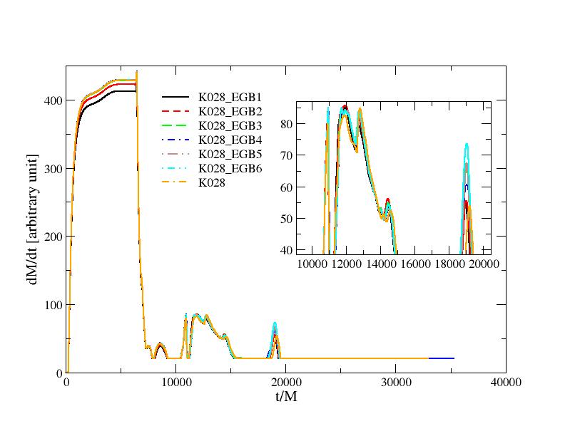
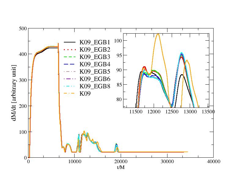
Figure 4: The mass accretion rates at the $r=3.88M$ point near the black hole horizon for different values of alpha EGB coupling constant $\alpha$. The mass accretion rates are plotted for the models with $a/M=0.28$ and $a/M=0.9$ given in Table 1, showing how the black hole’s spin parameter and $\alpha$ influence the mass accretion rate.

Figure 5 illustrates how the maximum density of the accretion disk around the black hole changes during the entire simulation for both $a/M=0.28$ and $a/M=0.9$. The results presented here are consistent with the mass accretion results shown in Fig.4. As mentioned earlier, and as can be also seen more clearly here, $\alpha$ has a significant impact on the stable disk formation process. This behavior has also been observed in Donmez (2023). In particular, it is observed that the maximum density corresponding to the biggest negative $\alpha$ values notably diverges from the others. However, although this divergence continues after perturbation, it is not as pronounced as before. For $a/M=0.9$, even though the higher values of $\alpha$ initially do not strongly affect the maximum density, we can observe this impact more distinctly during the $QPOs$ phase.

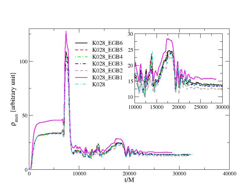
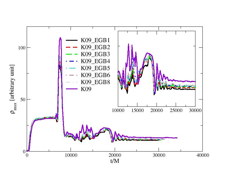
Figure 5: The time-dependent variation of the maximum density of the accretion disk around the black holes with the spin parameters $a/M=0.28$ and $a/M=0.9$. The inner plot illustrates more details about how the disk behaves until it reaches a quasi-steady-state after being perturbed.

5.3 Revealing the Instability of the Accretion Disk by Fourier Mode Analysis

Various factors such as gravitational influences, thermal conditions, and magnetic fields can cause instabilities in accretion disks. These instabilities have profound effects on the disk’s behavior, affecting the accretion rate onto the central object, radiation emission from the disk, and the generation of jets or outflows. Non-axisymmetric instabilities caused due to the gravitational influences predominantly arise in the equatorial plane and can be pinpointed and assessed via linear perturbation studies of the black hole-accretion disk system (Pierens, 2021). To characterize these instabilities, we define the azimuthal wavenumber $m$ and compute the saturation point using simulation data to calculate the Fourier power in density. We utilize equations provided by De Villiers & Hawley (2002); Dönmez (2014) to ascertain the Fourier modes $m=1$ and $m=2$ along with the growth rate at the equatorial plane $(i.e.,\theta=\pi/2)$. The imaginary and real parts of the Fourier mode are

$$Im(w_{m}(r))=\int_{0}^{2\pi}\rho(r,\phi)sin(m\phi)d\phi,$$ (9)

$$Re(w_{m}(r))=\int_{0}^{2\pi}\rho(r,\phi)cos(m\phi)d\phi.$$ (10)

The individual mode instability can be found by

$$P_{m}=\frac{1}{r_{out}-r_{in}}\int_{r_{in}}^{r_{out}}ln\left(\left[Re(w_{m}(r))\right]^{2}+\left[Im(w_{m}(r))\right]^{2}\right)dr,$$ (11)

where $r_{in}$ and $r_{out}$ are the inner and outer radii of the computational domain given in Section 3. However, instead of using the outer boundary position of the disk for $r_{out}$, it is chosen as $r_{out}\sim 35M$ to include the region where the gravitational field is strong and therefore the instability is dominant.

Here, we have revealed how instability grows in the perturbed stable disk for the models given in Table 1, whether it reaches saturation or not, and whether it enters a stable phase afterward. The numerical results in Fig.6 show that the behavior of the $m=1$ and $m=2$ modes is nearly the same for the black hole’s spin parameter $a/M=0.28$ and $a/M=0.9$ cases. In the left and right panels of Fig.6, it is evident that initially stable disks are observed. These disks reach a steady-state around $t=2000M$. The stable disk which is also seen in Fig.1 has been perturbed using the physical parameters given in Section 3 for the models in Table 1 at $t=6000M$. As seen in Fig.6, after perturbation, the stable disks become unstable, and for both models, the instability reaches a saturation around $t=8300M$. Right before reaching saturation, it is observed that $m=1$ and $m=2$ modes do not deviate significantly from each other.

Understanding $m=1$ and $m=2$ modes is crucial not only for revealing the characteristics of the emitted QPOs around a black hole but also for explaining observational results related to accretion disks (Shapiro et al., 1985; Li & Narayan, 2004). The $m=1$ mode illustrates the oscillation caused by matter spiraling inward toward the black hole. On the other hand, the $m=2$ mode can be utilized in describing the long-term structure of the disk and the properties of matter falling into the black hole. These modes are valuable tools in interpreting the behavior of accretion disks around the black holes.

Just before reaching the saturation point, both $m=1$ and $m=2$ modes has started to separate from each other in all models. For a while, both modes exhibite unstable behavior, moving downwards from the saturation point. Around $t=19000M$, the $m=2$ mode display stable oscillation, while instability continues in the $m=1$ mode. The $m=2$ mode maintains its stability until the end of the simulation, and towards the final stages of the calculation, the $m=1$ mode is also observed to transition to a steady-state. These stable modes oscillating around a fixed value demonstrate the existence of a one-armed spiral shock wave on the disk and a two-armed oscillation. These modes indicate that the black hole is regularly fed by matter, thus showing an increase in the black hole’s mass over time. At the same time, they continuously lead to the formation of $QPO$ frequencies.

The results presented here contributes to the numerical understanding of the formation of the massive black holes in the center of galaxies and AGNs, and the physical mechanisms that can lead to observed $QPOs$. This may help in providing a better explanation for observational data.

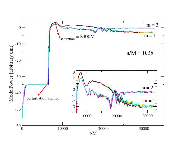
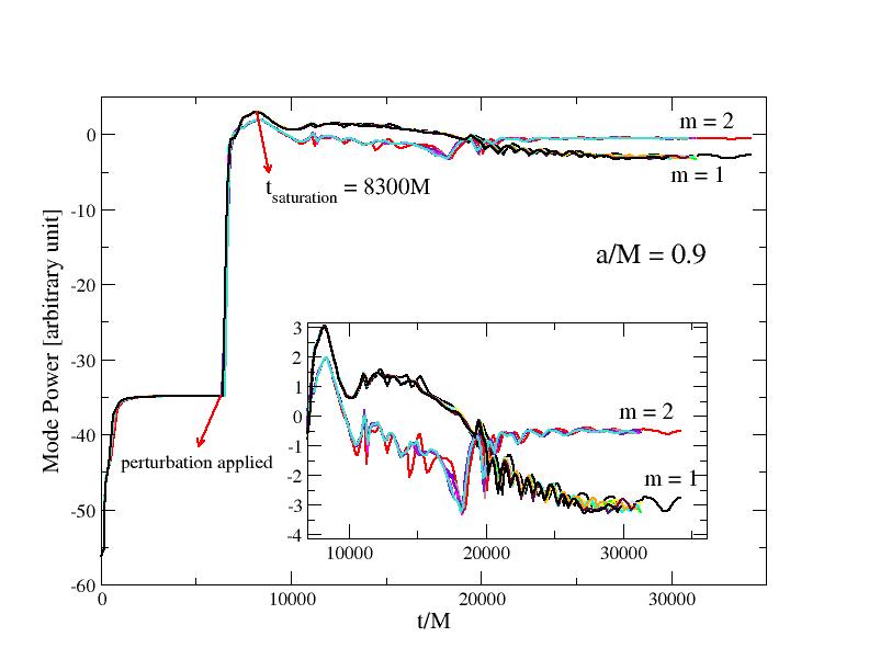
Figure 6: The behavior of modes ($m=1$ and $m=2$) for each of the two rotating black hole scenarios ($a/M=0.28$ and $a/M=0.9$) given in Table 1. Both modes reach saturation, and it has been observed that the $m=2$ mode reaches a steady-state faster than $m=1$.

5.4 QPOs in the Perturbed Disk

$GRS$ $1915+105$, situated in the Aquila constellation within our galaxy, is among the renowned $X-$ray binary systems. At its core lies a black hole, being fed by a companion star. As matter falls from the star towards the black hole, it disrupts the pre-existing stable accretion disk, resulting in the emission of high-energy $X-$rays and the presence of QPOs. QPOs of $GRS$ $1915+105$ exhibit a wide frequency range, spanning from a few $Hz$ to several hundred $Hz$, depending on their production location within the accretion disk. The truncated radius for these QPOs exhibits variation, spanning from approximately $1.24$ to about $19$ gravitational radii ($R_{g}$), relative to the last stable orbit of an almost maximally spinning black hole. Remarkably, the frequencies of the $C-$type QPOs, falling within the range of $2Hz$ to $6Hz$, conform closely to the pattern foreseen by the relativistic dynamical frequency model. An intriguing observation is that the high-frequency QPO at around $70Hz$ exhibits a similar behavior, implying that both types of QPOs likely stem from the innermost stable circular orbit, sharing a common underlying mechanism. This phenomenon aligns with what is observed in the more frequently observed $C-$type QPOs (Dhaka et al., 2023). The estimated mass of the $GRS$ $1915+105$ is around $12.4(+2.0,-1.8)M_{\odot}$ (Reid et al., 2014).

We performed a fast Fourier transform to compare the results obtained from numerical modeling with the observed source $GRS$ $1915+105$. We obtained oscillation frequencies by using the results derived from dumping the density values at a fixed point inside the shock cone where oscillation is excessive over time, or by using the time-dependent mass accretion rate taken at the inner boundary of the disk (near the black hole) in Fourier transformation. Then, to be able to show the obtained results in the frequency domain, we transform from the geometrized unit to the frequency domain using Eq.12

$$f(Hz)=f(M)\times 2.03\times 10^{5}\times\left(\frac{M\odot}{M}\right),$$ (12)

where $M$ represent the mass of the black hole. It has been chosen as $M=15M_{\odot}$ to compare the results obtained from the fast Fourier transform of numerical data with the observational results provided in the above sources. The numerical data is taken around $r=1.9R_{g}$ ($R_{g}$ is the gravitational radii), where the gravitational field is very strong.

The observation of frequencies generated by the oscillation due to the shock wave on the dynamic of the disk and their comparison with observed sources is essential for understanding the physical mechanisms that cause this emission in the observed sources. In this context, the power spectrum of the time-dependent mass accretion rate is calculated to identify the eigenmodes of oscillation during the formation, perturbation, and subsequent processes of the accretion disk. These are computed for different black hole spin parameters and EGB coupling constants, as shown in the Fig.7. The left and right panels illustrate how the oscillation frequencies of the disk around a slowly and fastly rotating black holes vary with different EGB coupling constants $\alpha$. For $a/M=0.28$ and $a/M=0.9$, it shows that the oscillation frequencies on the disk are nearly the same for different $\alpha$ values given in Table 1. Only for the highest negative value of alpha, the frequencies are slightly different. It is believed to be due to the highly chaotic motion discussed in section 5.6.

On the other hand, as seen in Fig.7 that the calculated frequencies have different magnitudes depending on the value of $\alpha$. It can be observed that the magnitude is larger for positive values of $\alpha$ compared to negative values. Since it’s easier to observe high-magnitude frequencies with telescopes, the observation results are likely to be in line with positive values of $\alpha$. The oscillation frequencies generated by the negative values may not be distinguishable from the background noise frequency.

Table 2: Frequencies of the first two genuine modes measured close to the black hole horizon from the evolution of the mass accretion rate. $a/M$ represents the black hole’s spin, $f_{1}$ corresponds to the first genuine mode, $f_{2}$ to the second genuine mode, and $Remarks$ indicates for which $\alpha$ values these are valid.

$a/M$	$f_{1}(Hz)$	$f_{2}(Hz)$	$Remarks$
$0.28$	$1.8$	$3.6$	$the\;same\;for\;all\;\alpha\;values$
$0.9$	$1.7$	$3.8$	$the\;same\;for\;all\;\alpha\;values$

Figure 7 displays the power spectrum frequencies resulting from genuine modes and their nonlinear couplings. Table 2 provides genuine modes for each case. These modes have been observed for every value of $\alpha$. Conversely, for the largest negative values of $\alpha$ , although the genuine modes are the same, the frequencies that later form as a result of nonlinear coupling differ from the other $\alpha$ cases. Furthermore, the separation of the frequencies following the genuine modes for the largest negative alpha value from those for other alpha values is evidence of the accretion disk exhibiting a more chaotic behavior.

As evident from the numerical results, both genuine modes and their nonlinear couplings can provide insights into the origin of the observed $QPOs$ in the source $GRS1915+105$. More specifically, the numerically observed genuine modes and their several nonlinear couplings fall within the observed range of $C-$type $QPO$ frequencies. These findings offer predictions regarding the nature of perturbations that could lead to the formation of these $QPOs$, as well as the potential physical characteristics of such perturbations.

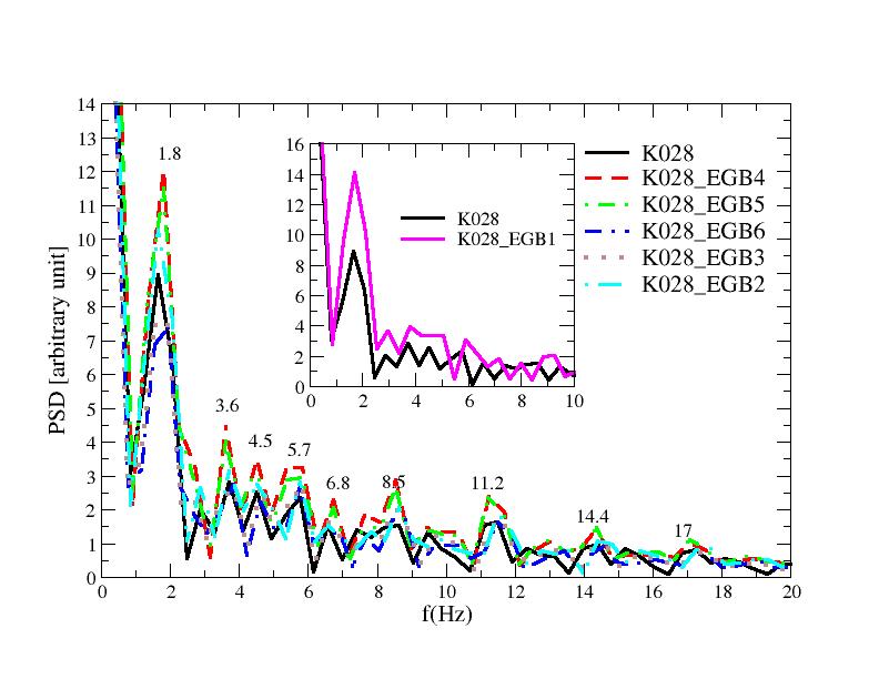
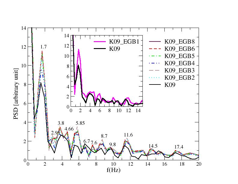
Figure 7: The power spectrum density (PSD) is calculated using the mass-accretion rate at $r=3.88M$ for a black hole with a mass $M=15M_{\odot}$. The graph on the left shows the frequencies of QPOs in the region near a rapidly rotating black hole with a spin parameter $a=0.9$ for the Kerr black hole and EGB black hole different values of coupling constant $\alpha$. The graph on the right, on the other hand, displays the QPO frequencies in the vicinity of a slowly rotating black hole with a spin parameter $a=0.28$.

5.5 Effect of Angular Momentum of the Perturbation on the Disk’s Dynamics

The stable accretion disk around the black hole experiencing perturbation at different initial angular speeds (rotational angular momentums) in the vicinity of the black hole leads to variations in the disk dynamics, the rate of change in the accretion rate, instabilities, characteristic of the strong shock waves, and consequently a change in the frequency of the emitted electromagnetic radiation (Long et al., 2022).

The left panel of Fig.8 shows that the change in mass-accretion rate over time significantly influences the formation and reaching of stability in the disk when the perturbation’s angular velocity is taken into account. After the stable disk is perturbed at $t=6000M$, it is observed that the matter around the black hole quickly either falls into the black hole or is ejected from the computational domain. This process continues until $t=8000M$. After this point, the two models exhibit completely different behaviors. The perturbation with zero angular velocity (K09_EGB9) quickly reaches a steady-state $(t=8500M)$, while the other one (K09_EGB8) oscillates until $t=19500M$. This illustrates that the physical properties of the perturbation have a significant impact on the formation, the accretion rate, and physical parameters of the disk around the black hole.

As seen in the right panel of Fig.8, in both systems, they quickly become unstable after perturbation. This instability increases rapidly in the early stages of the perturbation, growing until the mode value is approximately $3$. It reaches saturation here. Then, in the non-rotating perturbation case (K09_EGB9), the $m=1$ and $m=2$ modes oscillate around a certain value with a high amplitutude while showing a steady-state. However, this situation is entirely different in the case of perturbation with angular velocity (K09_EGB8). After saturation point, despite both modes of K09_EGB8 exhibiting unstable behavior, $m=2$ started to generate a stable oscillation at approximately $t=20000M$. This condition is maintained throughout the simulation time. On the other hand, it has been observed that $m=1$ reached an approximate steady-state towards the end of the calculation time and begin oscillating around a specific value. This also demonstrates that the single dominant mode of $m=1$ is insufficient to maintain the stable structure of the disk. In the case of a perturbation with angular velocity, as in $m=2$, having two dominant modes seems to ensure the stability of the disk, allowing it to reach a steady-state.

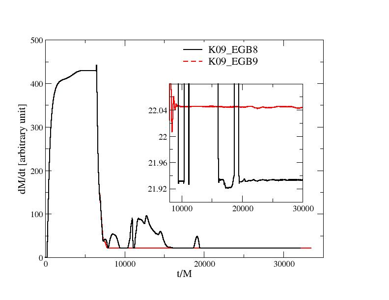
Figure 8: The models K09_EGB8 and K09_EGB9 are compared by calculating the mass-accretion rate and the oscillation mode powers of the disk. The behavior of perturbation with angular velocity appears to be more complex in relation to the physical parameters, and it seems that the accretion disk exhibits stronger non-linear oscillations compared to the non-rotating perturbation case.

Figure 9 illustrates how the density of the disk oscillates in the azimuthal direction $(\phi)$ over time, from the initial formation of the disk to the end of the simulation, at $r=3.88M$ for the K09_EGB8 (left panel) and K09_EGB9 (right panel) models. It is clear that the disk forms through spherical accretion up to $t=6000M$. After applying two different perturbations at $t=6000M$, the evolving behavior of the stable disk over time is evident. On the left panel, the oscillation of the disk resulting from the perturbation with angular velocity is shown, while the one with zero angular velocity presents disk oscillation. Here, it is clearly visible that the angular velocity of the matter sent as perturbation significantly affects the disk’s oscillation. This, in turn, leads to changes in various important physical parameters, such as oscillation modes, the physical characteristics of $X-$rays emitted in the region near the black hole, and the amount of matter falling into the black hole, etc.

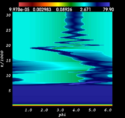
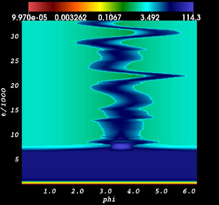
Figure 9: The time dependent variation of density as a function of $phi(\phi)$. The left one is for model K09_EGB8 and the right one is for K09_EGB9 at a constant $r=3.88M$. The effect of the angular velocity of the perturbation on the disk structure and the oscillation of the resulting shock wave is clearly observed.

Furthermore, Fig.10 demonstrates that different initial perturbation angular velocities lead to significant differences in observable oscillation frequencies. As expected, the frequencies obtained from the K09_EGB8 model, which exhibits more chaotic behavior, reveal a more chaotic structure, while the oscillation frequencies of the disk resulting from the non-rotating perturbation matter exhibit a more linear behavior. In addition, the oscillation frequencies obtained by taking the Fourier mode of the mass-accretion rate clearly appear much larger in the case of perturbation with zero angular velocity compared to the other. In addition, the amplitudes of the frequencies obtained from the K09_EGB8 model are nearly $10^{3}$ times stronger than the amplitudes of the genuine mode frequencies obtained from the other model. This facilitates the observation of these emissions by dedectors. Many telescopes can easily observe high-amplitude oscillations because they can distinguish them from background noise. Additionally, these types of oscillations carry more information about the black hole-disk system.

The oscillation frequencies obtained here have been compared with the observational results in sections 4 and 5.4. To make this comparison, $M=15M_{\odot}$ has been taken, which is approximately equivalent to the observed mass of the $GRS$ $1915+105$ black hole. As a result of the comparison, it has been observed that the results obtained from the perturbation with an angular momentum are in line with the observed results for the $GRS$ $1915+105$ source. More specifically, the genuine modes observed through numerical analysis, along with their numerous nonlinear interactions, align with the observed spectrum of $C-$type $QPO$ frequencies. This indicates that the frequency observed from this source is due to a perturbation with angular velocity of the perturbed disk. Therefore, the disk structure, the behavior of oscillation modes, and the physical characteristics of the disk obtained for the K09_EGB8 model can be used to explain the $GRS$ $1915+105$ source. The first two frequencies, $1.7Hz$ and $3.7Hz$, obtained from the Fourier spectrum of model K09_EGB8 given in the left side of Fig.10, are genuine eigenmodes. The others are modes resulting from their non-linear couplings. For example, the frequency $5.8Hz$ is equal to the sum of the first two genuine eigenmodes. These genuine eigenmodes and their non-linear coupling often produce ratios, such as $1:2:3$, and they fall within the observed frequency range of $GRS$ $1915+105$ and $C-$type QPOs.

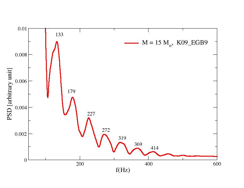
Figure 10: The same models are taken into account as seen in Fig.9, but this time, the oscillation frequencies on the disk are revealed using the mass-accretion rate at $r=3.88M$. The frequency axis is obtained using the mass of the black hole with $M=15M_{\odot}$

5.6 Exploring the Differences: Disk Dynamics under Kerr and EGB Gravities

It is evident that the different curvatures around the rotating black hole affect the dynamic structure of the forming disk and physical properties of the emitted $X-$ray. In this section, the influence of Kerr and EGB gravities on the disk structure has been elucidated.

The impact of the black hole’s spin parameter and the EGB coupling constants on the mass accretion rate of the disk is shown in Fig.4. As observed in the figure, the amount of matter falling from the disk towards the black hole is greater for non-zero values of $\alpha$ in the EGB gravity compared to Kerr gravity. This implies that for different values of $\alpha$, the disk feeds the black hole more, leading to the black holes having larger masses than those in Kerr gravity. When Fig.4 is examined in detail, it can be seen that this difference is very small for values of $\alpha$ close to zero, which is an expected result. On the other hand, it’s evident that a higher the mass accretion rate leads to a lower the maximum density in the disk, as seen in Fig.5.

Figure 7 displays the oscillation frequencies of $QPOs$ around the Kerr black holes and EGB gravity with different coupling constants. It is evident that, although the same frequencies are observed in both EGB and Kerr gravity scenarios, the amplitudes of the frequencies are greater in the EGB gravity cases. This enhances the detectability of these frequencies. Large-amplitude QPO oscillations are more likely to be detected by detectors due to their amplitude exceeding the background noise modes. At the same time, these oscillations help establish that their origin is not the result of numerical artifacts. On the other hand, for the most negative value of alpha (see the internal graphics in Fig.7), while the first genuine mode has the same frequency, subsequent modes differ from the Kerr gravity.

The occurrences of the shock waves in the dynamics structure of the accretion disk determine the severity of the disk instability. These types of the systems may exhibit consistent behavior at the same frequency which are valuable sources for observations. Here, to quantify the severity of the disk’s instability, we compute the ratio of the total time step at $t=30000M$ for each model to the total time step in the Kerr solution. This allows us to determine which systems require more time for calculations. Because, according to the Courant condition, the time step varies depending on, the instability occurred on the disk. In cases of severe instability, time step $dt$ decreases, leading to slower progress in time and differences in time steps within the same total time. As seen in Table 1, changes in the ratio of time steps can be observed depending on the chaos exhibited by the disk. The reasons for these changes include the fact that instability occurs only near the black hole throughout the entire simulation (which causes in a decrease in the total time step) or that the modelling of this instability affects the entire disk and is also influenced by the alternative gravity. All models have shown in Fig.11 that an increase in the negative direction of the EGB parameter $\alpha$ leads to the disk exhibiting a more chaotic behavior. As seen also in same figure that the black hole rotation parameter $a$ affect the accretion of the matter close the black hole horizon, and therefore, $a$ influences the chaotic structure of the disk. As observed in Fig.11, it is evident that $\alpha$ is not significantly effective in determining the chaotic behavior of a rapidly rotating black hole, particularly for values close to zero (both negative and positive). Therefore, for $a/M=0.9$, unexpected behavior has been observed for these $\alpha$ values. These chaotic structures can be used to explain intense continuous emissions from the black hole-disk systems and provides a wide frequency range in the emitted radiation (Misra et al., 2004; Guo et al., 2020). The amplitude of the radiation changes over time. They may be also source of sudden bursts (Cao et al., 2023). As seen in section 5.4, fundamental modes of oscillation create new frequencies by non-linear coupling. Thus, they may be suggested as a physical mechanism for the observed sources given in section 4.

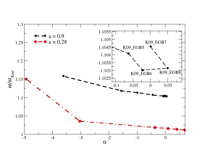
Figure 11: The ratio of the required time steps for each model to reach $t=30000M$ to the required time steps for a Kerr black hole at that time. The necessary time steps for each model have revealed the chaotic behavior of the accretion disk.

6 Discussion and Conclusion

In this study, we investigated the time variation of the accretion disks around the rotating black holes formed by Kerr and EGB gravities, depending on the black hole’s spin parameter ($a/M$) and the $EGB$ coupling constant ($\alpha$). We examine the effects of positive and negative values of $\alpha$ for both slowly-rotating ($a/M=0.28$) and fastly-rotating ($a/M=0.9$) black hole scenarios. This involves modeling the shock waves generated on the disk, the variation of intensities of the shock, changes in $QPO$ frequencies, and the chaotic structures they exhibited, all of which are dependent on these parameters.

A stable disk is perturbed by introducing matter from outside the computational domain at a specific point similar to $X-$ray binary system. If the perturbation is directed towards the black hole with a specific angular and radial velocities, it is observed that initially, a one-armed shock wave formed around the black hole, followed by the appearance of a two-armed shock wave. During this process, the disk begin exhibiting the non-linear oscillations. These shock waves are noted to persist even after their formation. However, it is observed that the disk exhibits a quasi-periodic oscillation before reaching the maximum simulation time. On the other hand, in the scenario where the perturbation has zero angular velocity, one- and two-armed shock waves still forms, but it is noticed that the oscillations are different characteristic behavior. These two different disk structures and oscillation conditions are found to significantly alter the QPO frequencies of the disk. In cases with zero angular velocity, the oscillation frequencies is observed in the hundreds and a few hundred Hz range. while the angular velocity is present at a specific value, these frequencies are found to be in the several Hz range. These frequencies have arisen from two genuine modes and their non-linear couplings. These genuine modes and the modes resulting from their non-linear couplings typically create ratios like $1:2:3$. There are some observed sources for these frequency ratios (Li & Narayan, 2004). Comparing the obtained QPO frequencies with observations led to the conclusion that the observed frequencies from the $GRS$ $1915+105$G black hole could be explained by the disk structure and shock waves generated by perturbations with angular velocity.

On the other hand, numerical calculations have strongly demonstrated that the mass accretion rate generated by perturbations with angular velocity is closely related with the black hole’s spin parameter ($a/M$) and EGB coupling constant ($\alpha$). Specifically, it has been observed that the mass accretion rate decreases (it causes an increase in the amount of matter falling into the black hole) due to the positive and negative variations in the $\alpha$ constant. Particularly, significant increases in this mass accretion rate have been clearly observed for large negative values of $\alpha$. As a result of this decrease, it has been observed that the disk density around the black hole and the intensity of the shock wave forming on it increase for both positive and negative $\alpha$ values. Therefore, it has been observed that the $QPO$ frequencies around the black holes have a wider range, with larger amplitudes for increasing $\alpha$. This, in turn, increases the likelihood of these frequencies being observed by telescopes.

The calculations here have shown that, as expected, instabilities grow shortly after the perturbation and reaches saturation. When describing these instabilities, both $m=1$ and $m=2$ modes are examined. Both modes exhibit instability for a certain period after reaching the saturation (Shapiro et al., 1985; Li & Narayan, 2004). Particularly, the $m=1$ mode, which characterizes a one-armed shock wave, showed instability for an extended period but eventually stabilized towards the end of the simulation. On the other hand, the $m=2$ mode, which characterizes a two-armed shock wave, exhibited quasi-periodic oscillations shortly after saturation and displayed stable behavior. These modes serve as evidence for the formation of shock waves in the numerically calculated disk. These shock waves are the physical mechanisms behind the observed QPOs. Using the disk structure presented here, it is possible to explain the causes of $QPOs$ in strong gravitational fields around different types of black holes, such as stellar and massive ones, that have not been discussed in this article.

In summary, the numerical results provided here can be applied to explain $QPOs$ observed in $X-$ray binaries, galaxies, and AGNs where the physical origins are yet to be fully understood or are subject to ongoing debates (Ingram & Motta, 2019; Song et al., 2020; Ren et al., 2023). These $QPOs$ result from the interaction between the black holes and disks at the centers of these systems and can be understood using the findings presented in this study. Finally, in the upcoming study, the physical characteristics of the perturbation provided in the $K09\_EGB8$ and $K09\_EGB9$ models will be explored over a broader parameter ranges, specifically around moderately rotating black holes. The impact of angular velocity on the disk dynamics and QPOs will be presented in greater detail in the forthcoming research.

References

- Abramowicz & Fragile (2013) Abramowicz, M. A., & Fragile, P. C. 2013, Living Reviews in Relativity, 16, 1, doi: 10.12942/lrr-2013-1
- Aoki et al. (2004) Aoki, S. I., Koide, S., Kudoh, T., Nakayama, K., & Shibata, K. 2004, ApJ, 610, 897, doi: 10.1086/421838
- Artymowicz & Lubow (1996) Artymowicz, P., & Lubow, S. H. 1996, ApJ, 467, L77, doi: 10.1086/310200
- Bowen et al. (2019) Bowen, D. B., Mewes, V., Noble, S. C., et al. 2019, ApJ, 879, 76, doi: 10.3847/1538-4357/ab2453
- Brogan et al. (2023) Brogan, R., Krumpe, M., Homan, D., et al. 2023, arXiv e-prints, arXiv:2307.14139, doi: 10.48550/arXiv.2307.14139
- Cao et al. (2023) Cao, X., You, B., & Wei, X. 2023, MNRAS, 526, 2331, doi: 10.1093/mnras/stad2877
- Chakrabarti et al. (2002) Chakrabarti, S. K., Acharyya, K., & Molteni, D. 2002, arXiv e-prints, astro, doi: 10.48550/arXiv.astro-ph/0211516
- De Villiers & Hawley (2002) De Villiers, J.-P., & Hawley, J. F. 2002, ApJ, 577, 866, doi: 10.1086/342238
- Dhaka et al. (2023) Dhaka, R., Misra, R., Yadav, J. S., & Jain, P. 2023, MNRAS, 524, 2721, doi: 10.1093/mnras/stad2075
- Ding et al. (2023) Ding, Q., Ji, L., Bu, Q.-C., Dong, T., & Chang, J. 2023, Research in Astronomy and Astrophysics, 23, 085024, doi: 10.1088/1674-4527/acdc88
- Dong et al. (2022) Dong, A., Liu, C., Zhi, Q., et al. 2022, Universe, 8, 273, doi: 10.3390/universe8050273
- Dönmez (2004) Dönmez, O. 2004, Ap&SS, 293, 323, doi: 10.1023/B:ASTR.0000044610.53714.95
- Dönmez (2006) —. 2006, International Journal of Modern Physics D, 15, 1001, doi: 10.1142/S0218271806008735
- Donmez (2006) Donmez, O. 2006, AM&C, 181, 256, doi: 10.1016/j.amc.2006.01.031
- Dönmez (2012) Dönmez, O. 2012, MNRAS, 426, 1533, doi: 10.1111/j.1365-2966.2012.21616.x
- Dönmez (2014) —. 2014, MNRAS, 438, 846, doi: 10.1093/mnras/stt2255
- Donmez (2022) Donmez, O. 2022, Physics Letters B, 827, 136997, doi: 10.1016/j.physletb.2022.136997
- Donmez (2023) —. 2023, arXiv e-prints, arXiv:2307.11725, doi: 10.48550/arXiv.2307.11725
- Donmez et al. (2022) Donmez, O., Dogan, F., & Sahin, T. 2022, Universe, 8, 458, doi: 10.3390/universe8090458
- Dönmez et al. (2011) Dönmez, O., Zanotti, O., & Rezzolla, L. 2011, MNRAS, 412, 1659, doi: 10.1111/j.1365-2966.2010.18003.x
- Donmez, Orhan (2021) Donmez, Orhan. 2021, Eur. Phys. J. C, 81, 113, doi: 10.1140/epjc/s10052-021-08923-1
- D’Orazio & Loeb (2018) D’Orazio, D. J., & Loeb, A. 2018, ApJ, 863, 185, doi: 10.3847/1538-4357/aad413
- Feng et al. (2022) Feng, M. Z., Kong, L. D., Wang, P. J., et al. 2022, ApJ, 934, 47, doi: 10.3847/1538-4357/ac7875
- Fernandes et al. (2022) Fernandes, P. G. S., Carrilho, P., Clifton, T., & Mulryne, D. J. 2022, Classical and Quantum Gravity, 39, 063001, doi: 10.1088/1361-6382/ac500a
- Gaskell & Goosmann (2013) Gaskell, C. M., & Goosmann, R. W. 2013, ApJ, 769, 30, doi: 10.1088/0004-637X/769/1/30
- Guo et al. (2020) Guo, X., Liang, K., Mu, B., Wang, P., & Yang, M. 2020, European Physical Journal C, 80, 745, doi: 10.1140/epjc/s10052-020-8335-6
- Ingram & Motta (2019) Ingram, A. R., & Motta, S. E. 2019, New A Rev., 85, 101524, doi: 10.1016/j.newar.2020.101524
- Jin et al. (2023) Jin, Y. J., Wang, W., Chen, X., et al. 2023, arXiv e-prints, arXiv:2306.13994, doi: 10.48550/arXiv.2306.13994
- Khan et al. (2016) Khan, F. M., Fiacconi, D., Mayer, L., Berczik, P., & Just, A. 2016, ApJ, 828, 73, doi: 10.3847/0004-637X/828/2/73
- Kim et al. (2018) Kim, D. C., Yoon, I., & Evans, A. S. 2018, ApJ, 861, 51, doi: 10.3847/1538-4357/aac77d
- Li & Narayan (2004) Li, L.-X., & Narayan, R. 2004, ApJ, 601, 414, doi: 10.1086/380446
- Long et al. (2022) Long, F., Yang, M., Chen, J., & Wang, Y. 2022, International Journal of Modern Physics A, 37, 2250206, doi: 10.1142/S0217751X22502062
- McHardy (2010) McHardy, I. 2010, in Lecture Notes in Physics, Berlin Springer Verlag, ed. T. Belloni, Vol. 794, 203, doi: 10.1007/978-3-540-76937-8_8
- Miller et al. (2012) Miller, J. M., Raymond, J., Fabian, A. C., et al. 2012, ApJ, 759, L6, doi: 10.1088/2041-8205/759/1/L6
- Misra et al. (2004) Misra, R., Harikrishnan, K. P., Mukhopadhyay, B., Ambika, G., & Kembhavi, A. K. 2004, ApJ, 609, 313, doi: 10.1086/421005
- Mohammed et al. (2023) Mohammed, N., Runnoe, J., Eracleous, M., et al. 2023, in American Astronomical Society Meeting Abstracts, Vol. 55, American Astronomical Society Meeting Abstracts, 360.07
- Motta & Belloni (2023) Motta, S. E., & Belloni, T. M. 2023, arXiv e-prints, arXiv:2307.00867, doi: 10.48550/arXiv.2307.00867
- Nixon et al. (2011) Nixon, C. J., King, A. R., & Pringle, J. E. 2011, MNRAS, 417, L66, doi: 10.1111/j.1745-3933.2011.01121.x
- Palenzuela et al. (2010) Palenzuela, C., Lehner, L., & Liebling, S. L. 2010, Science, 329, 927, doi: 10.1126/science.1191766
- Petrich et al. (1989) Petrich, L. I., Shapiro, S. L., Stark, R. F., & Teukolsky, S. A. 1989, ApJ, 336, 313, doi: 10.1086/167013
- Pierens (2021) Pierens, A. 2021, MNRAS, 504, 4522, doi: 10.1093/mnras/stab183
- Rana & Mangalam (2020) Rana, P., & Mangalam, A. 2020, ApJ, 903, 121, doi: 10.3847/1538-4357/abb707
- Reid et al. (2014) Reid, M. J., McClintock, J. E., Steiner, J. F., et al. 2014, ApJ, 796, 2, doi: 10.1088/0004-637X/796/1/2