Long Solution Times or Low Solution Quality: On Trade-Offs in Choosing a Power Flow Formulation for the Optimal Power Shut-Off Problem

Abstract

The Optimal Power Shutoff (OPS) problem is an optimization problem that makes power line de-energization decisions in order to reduce the risk of igniting a wildfire, while minimizing the load shed of customers. This problem, with DC linear power flow equations, has been used in many studies in recent years. However, using linear approximations for power flow when making decisions on the network topology is known to cause challenges with AC feasibility of the resulting network, as studied in the related contexts of optimal transmission switching or grid restoration planning. This paper explores the accuracy of the DC OPS formulation and the ability to recover an AC-feasible power flow solution after de-energization decisions are made. We also extend the OPS problem to include variants with the AC, Second-Order-Cone, and Network-Flow power flow equations, and compare them to the DC approximation with respect to solution quality and time. The results highlight that the DC approximation overestimates the amount of load that can be served, leading to poor de-energization decisions. The AC and SOC-based formulations are better, but prohibitively slow to solve for even modestly sized networks thus demonstrating the need for new solution methods with better trade-offs between computational time and solution quality.

This work is supported by the U.S. National Science Foundation ASCENT program under award 2132904.

I Introduction

Climate change is expected to increase the risk of wildfires in many parts of the world [1]. In recent years, several large and devastating fires ignited by power lines have increased scrutiny on utility practices to avoid wildfire ignitions. In California, utilities are routinely leveraging de-energization of power lines – commonly referred to as public safety power shut-offs (PSPS) – as a measure to prevent fires (and limit their liability) during periods of extreme risk. While PSPS is effective at reducing wildfire ignitions [2], it carries a significant cost in customer outages . Prior work has considered how to optimally implement PSPS, a problem called Optimal Power Shutoff (OPS), to balance the wildfire risk reduction with the resulting load shed [3], reduce PSPS-caused power outages through energy storage [4, 5] or microgrids [6][7], or transmission upgrades [8, 9, 10].

A common aspect of prior work is that they all rely on a DC power flow approximation to reduce computational time. However, DC power flow does not account for reactive power flows and voltage constraints, and produces solutions that are not AC power flow feasible [11]. This is particularly true when the system is operating under stress, as can be expected when a substantial number of lines are switched off during a power shut-off. Some data-driven methods for power management during high risk wildfire use AC power flow, but only considers up to three de-energizations in the network [12].

The goal of this paper is to assess how the choice of a power flow representation in the OPS problem impacts solution quality, solution time, and the trade-off between the two. While this is a question that is important for the OPS problem, it also arises in many other power system optimization problems which involve binary decisions regarding whether or not certain transmission lines should be in operation. Examples include transmission switching [13], maintenance planning [14], and transmission expansion [15]. It is known that using DC power flow in transmission switching may produce infeasible or sub-optimal solutions, and some methods correct DC models for AC-infeasiblility [16] or use convex relaxations such as Second-Order-Cone (SOC) [17] to address this limitation. It is worth noting that existing methods for AC-feasibility recovery from DC-based solutions or heuristic solutions to transmission switching [18, 19, 20] are not directly applicable to OPS problems because OPS problems 1) tend to turn off many more power lines, 2) may involve load shed, and 3) may split the system into multiple islands.

Other problems are more closely related to the OPS problem in that large regions of the grid may be de-energized, the network may contain islands, and load shed may be required to find feasible power flow solutions. Examples include the Maximal Load Delivery (MLD) problem in a severely damaged power system [21], where some lines may have to be disconnected for feasibility, as well as the associated problem of post-disaster restoration [22, 23], which decides which lines among a set of damaged lines should be prioritized for repair. Both [22, 23] and  [21] include investigations into the choice of power flow formulations. They demonstrate that DC power flow may lead to sub-optimal binary decisions due to lack of consideration of reactive power and voltage problems, and that AC-based formulations may get stuck in local optima. SOC-based formulations seem to provide the best accuracy-quality trade-off given current solver technology, but can still be prohibitively slow. The results in [22] also demonstrated the need to redispatch generation with an AC-based optimal power flow after the binary decisions are made.

In this paper, we leverage the experiences from prior work to study the solution accuracy, ability to recover an AC feasible solution and solution speed in the context of the OPS problem. This problem differs from MLD and restoration problems in that we choose which power lines to de-energize from all lines in the system (as opposed to outage scenarios where a limited number of outaged lines are given) and that it contains a different objective with multiple parts (i.e. to balance wildfire risk reductions with load shed). Furthermore, prior work [24] has shown that the partially de-energized grids tend to have a primarily radial structure. These differences may have significant impact on the solution speed and accuracy of approximations at the optimal solution, and thus warrants an independent evaluation. We also found that prior methods for AC-feasibility recovery failed in many cases, leading us to devise a more comprehensive feasibility recovery process.

In summary, the contributions of the work are as follows. 1) We develop the formulations of the OPS problem that use the AC, SOC, Network Flow (NF), and DC power flow formulations. 2) We devise a process for recovering AC-feasible power flow solutions to the OPS de-energization decisions, leveraging both a continuous AC-Redispatch problem and mixed-integer MLD problem. 3) We perform a comprehensive analysis of solution time and solution quality using 11 test networks with hundreds of risk scenarios. We assess the objective values and accuracy of solutions obtained with different power flow formulations, as well as the solution time.

The remainder of the paper is organized as follows: Section II introduces the OPS problem formulations and Section III introduce the AC-feasible power flow recovery. Section IV analyzes the impact of power flow formulation on OPS, and Section V concludes the work.

II Optimal Power Shutoff Problem Formulation

In this section we introduce the OPS problem with AC, SOC, DC, and Network-Flow (NF) power flow formulations. The formulation is based on the DC-OPS problem that was first presented in [3], while the adaptation to AC, SOC and NF formulations are new.

Across formulations, we consider a network with buses $i\in\mathcal{B}$, generators $g\in\mathcal{G}$, lines $ij\in\mathcal{L}$, and load $d\in\mathcal{D}$. Subsets of components such as generators at bus $i$ are defined as $\mathcal{B}^{\mathcal{G}}_{i}$. Parameters are bold while variables are non-bold. Binary variables representing the energization state of a component are $z\in\{0,1\}$ and indexed according to the component. If $z\!\!=\!\!1$, the component is energized, otherwise $z\!=\!0$.

II-A AC Optimal Power Shutoff

We start by defining the OPS problem with AC power flow equations, then show how the formulation must adapt for the other power flow formulations.

II-A1 Objective function

The objective of the OPS problem seeks to maximize the power delivered while minimizing the risk of a wildfire ignition, with a pre-specified weighting factor $\bm{\alpha}\in[0,1]$ to determine a trade-off between load delivery and risk reduction. The objective function is given by

$$\max\;\;(1-\bm{{\alpha}})\frac{\sum_{d\in\mathcal{D}}x_{d}w_{d}\bm{P}^{D}_{d}}{\bm{P}^{D}_{tot}}+\bm{{\alpha}}\frac{\sum_{ij\in\mathcal{L}}z_{ij}\bm{R}_{ij}}{\bm{R}_{tot}}$$ (1)

The first term represents the total power delivered in the system. The power delivered to each node $d$ is given by the power demand $\bm{P}_{d}^{D}$ multiplied by the continuous variable $x_{d}\in[0,1]$. The weighting factor $w_{d}$ can be used to prioritize loads such as emergency services and community centers.

The second term represents the risk of wildfire ignitions. The risk associated with an ignition from line $ij$ is given by parameter $\bm{R}_{ij}$, which is multiplied by the binary energization status of a power line $z_{ij}$. If the line is de-energized, $z_{ij}=0$ and the risk is set to zero as a de-energized power line cannot ignite a wildfire. If the line remains energized, $z_{ij}=1$ and the line has a non-zero risk. The total wildfire ignition risk is the summation over all power lines. The two terms are normalized by the total load demand $\bm{P}^{D}_{tot}=\sum_{d\in\mathcal{D}}\bm{P}^{D}_{d}$ and total wildfire risk $\bm{R}_{tot}=\sum_{ij\in\mathcal{L}}\bm{R}_{ij}$ in the system, respectively.

II-A2 Energization constraints

Each component in the system can be de-energized to reduce wildfire risk and achieve a feasible power flow solution. However, the ability to energize or de-energize certain components also depends on the status of the components they are connected to. Specifically, if a bus $i$ is de-energized $z_{i}=0$, any connected loads has to be shed (i.e. $x_{d}=0$), and all generators and lines have to be de-energized (i.e. $z_{g}=0$ and $z_{ij}=0$). These relationships are described by the following constraints,

$$x_{d}\leq z_{i} \forall d\in\mathcal{B}^{\mathcal{D}}_{i},\;\forall i\in\mathcal{B}$$ (2a)

$$z_{ig}\leq z_{i} \forall g\in\mathcal{B}^{\mathcal{G}}_{i},\;\forall i\in\mathcal{B}$$ (2b)

$$z_{ij}\leq z_{i} \forall ij\in\mathcal{B}_{i}^{\mathcal{L}},\;\forall i\in\mathcal{B}$$ (2c)

II-A3 Generation constraints

The active power output of a generator $P_{g}^{G}$ is constrained between is upper $\overline{\bm{P}^{G}_{g}}$ and lower $\underline{\bm{P}^{G}_{g}}$ power limits when the generator is energized, and constrained to $0$ when the generator is de-energized, Eq. (3). The reactive power is similarly constrained in eq. (4).

$$z_{g}\underline{\bm{P}^{G}_{g}}\leq P_{g}^{G}\leq z_{g}\overline{\bm{P}^{G}_{g}}\quad\forall g\in\mathcal{G}$$ (3)

$$z_{g}\underline{\bm{Q}^{G}_{g}}\leq Q_{g}^{G}\leq z_{g}\overline{\bm{Q}^{G}_{g}}\quad\forall g\in\mathcal{G}$$ (4)

II-A4 Power flow constraints

Active and reactive power balance at each node are given by

$$\sum_{g\in\mathcal{B}_{i}^{\mathcal{G}}}P_{g}^{G}-\!\!\!\!\!\!\sum_{(i,j)\in\mathcal{B}_{i}^{\mathcal{L}}}\!\!\!\!\!P_{ij}^{L}-\!\!\!\!\sum_{d\in\mathcal{B}_{i}^{\mathcal{D}}}\!\!\!x_{d}\bm{P}^{D}_{d}=0\quad\forall i\in\mathcal{B}$$ (5)

$$\sum_{g\in\mathcal{B}_{i}^{\mathcal{G}}}Q_{g}^{G}-\!\!\!\!\!\!\sum_{(i,j)\in\mathcal{B}_{i}^{\mathcal{L}}}\!\!\!\!\!Q_{ij}^{L}-\!\!\!\!\sum_{d\in\mathcal{B}_{i}^{\mathcal{D}}}\!\!\!x_{d}\bm{Q}^{D}_{d}=0\quad\forall i\in\mathcal{B}$$ (6)

where $Q_{g}^{G}$ is the generator reactive power, $P_{ij}^{L},Q_{ij}^{L}$ represent the active and reactive power flow on line $ij$ and $\bm{Q}_{d}^{D}$ is the reactive power demand. The thermal power limit for a power line $\bm{T}_{ij}$ is expressed in terms of the squared magnitude of complex power, which must be between the squared thermal limit of the power line when energized $z_{ij}=1$, or set to $0$ when the line is de-energized $z_{ij}=0$. This is given by

$$-\bm{T}_{ij}^{2}z_{ij}\leq(P_{ij}^{L})^{2}+(Q_{ij}^{L})^{2}\leq\bm{T}_{ij}^{2}z_{ij}\quad\forall ij\in\mathcal{L}$$ (7)

The bus voltage magnitude $V_{i}$ must be within the upper $\bm{\overline{V}}_{i}$ and lower $\bm{\underline{V}}_{i}$ limits when bus $i$ is energized, and $0$ otherwise,

$$z_{i}\bm{\underline{V}}_{i}\leq V_{i}\leq z_{i}\bm{\overline{V}}_{i}\quad\forall i\in\mathcal{B}$$ (8)

The AC power flow equations with line switching are

$$\!\!\!P_{ij}^{L}\!\!=\!\!z_{ij}\!\left(\bm{g}_{ij}V_{i}V_{j}\cos\!\left(\theta_{i}\!\!-\!\!\theta_{j}\right)\!\!+\!\!\bm{b}_{ij}V_{i}V_{j}\sin\!\left(\theta_{i}\!\!-\!\!\theta_{j}\right)\right)\forall ij\!\in\!\mathcal{L}$$ (9a)

$$\!\!\!\mkern-1.0muQ_{ij}^{L}\!\!=\!\!z_{ij}\!\left(\bm{g}_{ij}V_{i}V_{j}\sin\!\left(\theta_{i}\!\!-\!\!\theta_{j}\right)\!\!-\!\!\bm{b}_{ij}V_{i}V_{j}\cos\!\left(\theta_{i}\!\!-\!\!\theta_{j}\right)\right)\forall ij\!\in\!\mathcal{L}$$ (9b)

Here, $\bm{g}_{ij}$ and $\bm{b}_{ij}$ are the conductance and suseptance, and $V_{i},V_{j}$ and $\theta_{i},\theta_{j}$ are the voltage magnitudes and angles at either end of the power line. When the a power line is energized $z_{ij}=1$ the equations represent ordinary AC power flow, while the power flow across the line is constrained to 0 when the line is de-energized $z_{ij}=0$.

The voltage angle difference between two ends of a line must be between the maximum angle difference limits of the power line when the line is energized, and should be unconstrained when the line is de-energized. This is expressed by the following big-M constraint,

$$\theta_{i}-\theta_{j}\leq\overline{\bm{\theta}_{ij}}+\bm{\theta}^{\Delta}_{max}(1-z_{ij})$$ (10a)

$$\theta_{i}-\theta_{j}\geq\underline{\bm{\theta}_{ij}}-\bm{\theta}^{\Delta}_{max}(1-z_{ij})$$ (10b)

Here, $\bm{\theta}^{\Delta}_{max}$ is pre-computed to be the maximum angle difference between any two buses in the power system and used as the big-M value. The above equations are used to define the AC Optimal Power Shutoff (AC-OPS) problem, i.e.

$$\max$$ Objective (1)

s.t.: $$\mbox{Component relationships:}~{}\eqref{eq:ops_relationships}$$

$$\mbox{Generation constraints:}~{}\eqref{eq:ops_active_gen_limits},\eqref{eq:ops_reactive_gen_limits}$$

$$\mbox{AC Power flow constraints:}~{}\eqref{eq:ops_active_power_balance}-\eqref{eq:ops_voltage_angle}$$

This is a mixed-integer non-linear (and non-convex) problem (MINLP), which is a challenging class of problems to solve.

II-B SOC Optimal Power Shutoff

We next describe the SOC-OPS problem, which uses the SOC relaxation of AC power flow, such that the objective value of the formulation is an upper bound on the optimal solution. The SOC power flow equations with component switching are adopted from [21]. Here we focus on just describing the variables and constraints that differ from the AC power flow formulation, and refer the reader [25] for details on the derivation of the SOC relaxation. To obtain a convex relaxation of the power flow equations, the SOC formulation represent products between voltages $V_{i}$ and $V_{j}$ using a set of lifted voltage squared variables $W_{ij}$, with real and imaginary components given by $W_{ij}^{R}$, $W_{ij}^{I}$. The formulation does not contain voltage angle variables. The upper and lower bounds on these variables are constrained by

$$z_{ij}\bm{\underline{V}}_{i}\bm{\underline{V}}_{j}\cos(\bm{\overline{\theta}}_{ij})\!\leq\!W^{R}_{ij}\!\leq\!z_{ij}\bm{\overline{V}}_{i}\bm{\overline{V}}_{j}\cos(\bm{\underline{\theta}}_{ij}) \!\!\!\!\!\forall ij\in\mathcal{L}$$ (11a)

$$z_{ij}\bm{\overline{V}}_{i}\bm{\overline{V}}_{j}\sin(\bm{\underline{\theta}}_{ij})\!\leq\!W^{I}_{ij}\!\leq\!z_{ij}\bm{\underline{V}}_{i}\bm{\underline{V}}_{j}\sin(\bm{\overline{\theta}}_{ij}) \!\!\!\!\!\forall ij\in\mathcal{L}$$ (11b)

Note that the limits are multiplied by the energization state of the power line $z_{ij}$ which constrains the voltage to $0$ when the power line is de-energized. The SOC power flow equations with line switching are given by

$$P_{ij}^{L}=z_{ij}\left(\bm{g}_{ij}W^{R}_{ij}+\bm{b}_{ij}W^{I}_{ij}\right) \forall ij\in\mathcal{L}$$ (12a)

$$Q_{ij}^{L}=z_{ij}\left(\bm{g}_{ij}W^{I}_{ij}-\bm{b}_{ij}W^{R}_{ij}\right) \forall ij\in\mathcal{L}$$ (12b)

Again, the power flow is multiplied by the state of the power line $z_{ij}$ to ensure power flow is set to $0$ when the line is de-energized. With this, the full SOC-OPS formulation is

$$\max$$ Objective (1)

s.t.: $$\mbox{Component relationships:}~{}\eqref{eq:ops_relationships}$$

$$\mbox{Generation constraints:}~{}\eqref{eq:ops_active_gen_limits},\eqref{eq:ops_reactive_gen_limits}$$

$$\mbox{SOC Power flow constraints:}~{}\eqref{eq:ops_active_power_balance}-\eqref{eq:ops_complex_thermal_limit},\eqref{eq:ops_soc_voltage_magnitude},\eqref{eq:ops_soc_powerflow}$$

This is a mixed-integer second-order cone problem (MISOCP). It is convex and thus easier to solve than the AC-OPS, but still a very challenging problem class.

II-C DC Optimal Power Shutoff

The DC-OPS problem is the original version first proposed in [3]. It uses the DC power flow linear approximation to model the power flow, which only considers real power and does not model reactive power or voltage constraints. The power flow $P_{ij}^{L}$ is constrained be lower than the thermal limit $\bm{T}_{ij}$ when the line is energized, and to $0$ when the power line is de-energized, as described by

$$-\bm{T}_{ij}z_{ij}\leq P_{ij}^{L}\leq\bm{T}_{ij}z_{ij}\quad\forall ij\in\mathcal{L}$$ (13)

The DC power flow equations with line switching are

$$P_{ij}^{L}\leq-\bm{b}_{ij}(\theta_{i}-\theta_{j}+\bm{\theta}^{\Delta}_{max}(1-z_{ij})) \forall ij\in\mathcal{L}$$ (14a)

$$P_{ij}^{L}\geq-\bm{b}_{ij}(\theta_{i}-\theta_{j}-\bm{\theta}^{\Delta}_{max}(1-z_{ij})) \forall ij\in\mathcal{L},$$ (14b)

which simplify to the standard DC power flow when the line is energized $z_{ij}=1$, and ensures that the voltage angle difference $\theta_{i}-\theta_{j}$ is unconstrained when the line is de-energized by introducing the big-M value from (10). The full DC OPS problem is given by

$$\max$$ Objective (1)

s.t.: $$\mbox{Component relationships:}~{}\eqref{eq:ops_relationships}$$

$$\mbox{Generation constraints:}~{}\eqref{eq:ops_active_gen_limits}$$

$$\mbox{DC Power flow constraints:}~{}\eqref{eq:ops_active_power_balance},\eqref{eq:ops_voltage_angle},\eqref{eq:ops_active_thermal_limit},\eqref{eq:ops_dc_powerflow}$$

The DC-OPS is a mixed-integer linear problem (MILP) which is easier than the above two problems, but still challenging to solve for large cases.

II-D NF Optimal Power Shutoff

The Network Flow OPS problem replaces the physics based power flow equations with a network flow model [26]. This model considers active power conservation on each node and assumes that power can be sent along any edge as long as the transmission capacity constraint (13) is respected. The resulting optimization model is given by

$$\max$$ (1)

s.t.: $$\mbox{Component relationships:}~{}\eqref{eq:ops_relationships}$$

$$\mbox{Generation constraints:}~{}\eqref{eq:ops_active_gen_limits}$$

$$\mbox{Network flow constraints:}~{}\eqref{eq:ops_active_power_balance},\eqref{eq:ops_active_thermal_limit} \eqref{eq:ops_relationships}\eqref{eq:ops_active_gen_limits}\eqref{eq:ops_active_power_balance}\eqref{eq:ops_active_thermal_limit}$$

Similar to the DC-OPS, the NF-OPS is also a mixed-integer linear program (MILP), though with fewer constraints.

III Recovering AC Feasible Solutions

The above OPS formulations determine a set of binary de-energization decisions for each line, as well as a set of continuous variables that describe the generation, load and power flow in the system. Since the solutions obtained with SOC, DC and NF formulations are typically not AC-feasible, the load shed predicted by the optimization problem for the given de-energization solution may be wrong. To evaluate the true load shed amount, we seek to identify the minimum AC-feasible load shed (or, conversely, the maximum AC-feasible load delivery) for the set of de-energization decisions determined by those formulations. Our approach to recover an AC feasible solution leverages the AC-Redispatch problem [22] and the Maximal Load Delivery (MLD) problem [21] to find an AC-feasible power flow. We first introduce the formulation of these optimizations problems, then describe the process for recovering the AC-feasible power flow.

III-A AC-Redispatch

The AC-Redispatch problem is a continuous AC optimal power flow which maximizes the load served, i.e.,

$$\max\qquad\sum_{d\in\mathcal{D}}x_{d}w_{d}\bm{P}_{d}$$ (15)

We solve this problem with the de-energization decisions fixed to the values $\bm{\hat{z}}$ from an OPS solution,

$$z_{ij}=\bm{\hat{z}}_{ij} \forall ij\in\mathcal{L}$$ (16a)

$$z_{i}=\bm{\hat{z}}_{i} \forall i\in\mathcal{B}$$ (16b)

$$z_{g}=\bm{\hat{z}}_{g} \forall g\in\mathcal{G}$$ (16c)

For conciseness of notation, we use the same equations used in the AC-OPS problem, with added constraints to fix the binary values to the energization state from the solution of an OPS problem, shown in (16). In practice, this problem is modeled as a continuous NLP problem rather than a MINLP problem. The full AC-Redispatch problem is given by

$$\max \eqref{eq:load_objective}$$

s.t.: $$\mbox{Component relationships:}~{}\eqref{eq:redis_fixed}$$

$$\mbox{Generation constraints:}~{}\eqref{eq:ops_active_gen_limits},\eqref{eq:ops_reactive_gen_limits}$$

$$\mbox{AC Power flow constraints:}~{}\eqref{eq:ops_active_power_balance}-\eqref{eq:ops_voltage_angle}$$

III-B Maximal Load Delivery

In some situations, the de-energization solution $\bm{\hat{z}}$ may not admit an AC-feasible solution. In this case, we solve the Maximal Load Delivery Problem (MLD) [21] problem to determine the maximum amount of load that can be served. This optimization problem is similar to the AC-Redispatch, but allow de-energization of additional components as modelled by the following constraints,

$$z_{ij}\leq\bm{\hat{z}}_{ij} \forall ij\in\mathcal{L}$$ (17a)

$$z_{i}\leq\bm{\hat{z}}_{i} \forall i\in\mathcal{B}$$ (17b)

$$z_{g}\leq\bm{\hat{z}}_{g} \forall g\in\mathcal{G}$$ (17c)

The AC power flow formulation of the MLD problem is

$$\max \eqref{eq:load_objective}$$

s.t.: $$\mbox{Component relationships:}~{}\eqref{eq:ops_relationships},\eqref{eq:mld_status}$$

$$\mbox{Generation constraints:}~{}\eqref{eq:ops_active_gen_limits},\eqref{eq:ops_reactive_gen_limits}$$

$$\mbox{AC Power flow constraints:}~{}\eqref{eq:ops_active_power_balance}-\eqref{eq:ops_voltage_angle}$$

The AC-MLD formulation is an MINLP, a similar problem class as the AC-OPS, and can be very computationally challenging. Our AC-feasibility recovery process therefore also leverages a version of the MLD based on SOC power flow, the SOC-MLD, which is a MISOCP of similar complexity as the SOC-OPS. The formulation of this problem is given by

$$\max \eqref{eq:load_objective}$$

s.t.: $$\mbox{Component relationships:}~{}\eqref{eq:ops_relationships},\eqref{eq:mld_status}$$

$$\mbox{Generation constraints:}~{}\eqref{eq:ops_active_gen_limits},\eqref{eq:ops_reactive_gen_limits}$$

$$\mbox{SOC Power flow constraints:}~{}\eqref{eq:ops_active_power_balance}-\eqref{eq:ops_complex_thermal_limit},\eqref{eq:ops_soc_voltage_magnitude},\eqref{eq:ops_soc_powerflow}$$

III-C AC Recovery Method

Given the above problem formulations, we propose the following algorithm to recover an AC-feasible solution. This algorithm starts by attempting to recover a solution by using less computationally intensive methods,

Step 1: Solve AC-Redispatch We solve the AC-Redispatch problem using the de-energization decisions $\hat{z}$ from the respective OPS problem. If the AC-Redispatch is feasible, we terminate the algorithm and return the power flow solution and amount of load shed. Otherwise, move to the next step.

Step 2: Solve SOC-MLD We solve the SOC-MLD problem with $\hat{z}$ from the OPS problem as an input. The resulting set of de-energized components ${z^{*}}$ may include additional de-energized elements. Using ${z^{*}}$, we then solve the AC-Redispatch problem. If the AC-Redispatch is feasible, we report the power flow and load shed. Otherwise, we move to the next step.

Step 3: Solve AC-MLD As a final step, we resort to solving the computationally challenging AC-MLD problem. If this problem finds a feasible solution, we report the power flow and load shed. If the problem does not solve within the allocated 1 hour time limit, we terminate the algorithm by reporting the trivial solution with a 0% load delivery as the AC-feasible solution.

The difficulty of recovering a feasible solution depends on the the complexity of the optimization problem that is required. For example, it is relatively quick if the only necessary step is to solve the AC-Redispatch problem. If the MLD problem is required, then we must solve an MISOCP or potentially an MINLP problem, which can be very slow and of similar complexity as solving the AC-OPS directly. If we solve the OPS problem the a MILP formulation, but require a difficult MINLP problem to recover an AC-feasible power flow, it defeats the purpose of having a faster OPS implementation.

IV Case Study

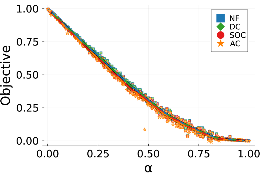
(a)

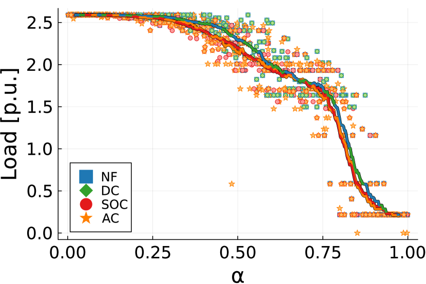
(b)

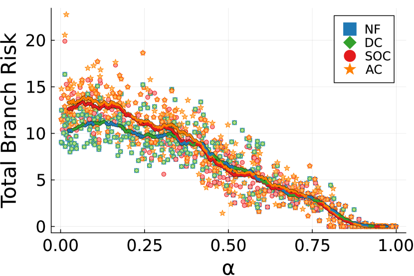
(c)

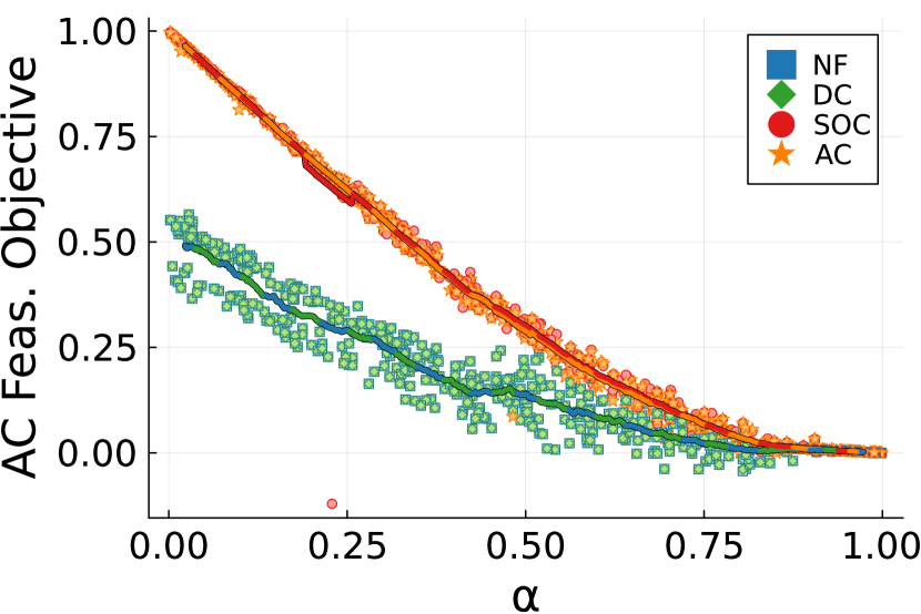
(d)

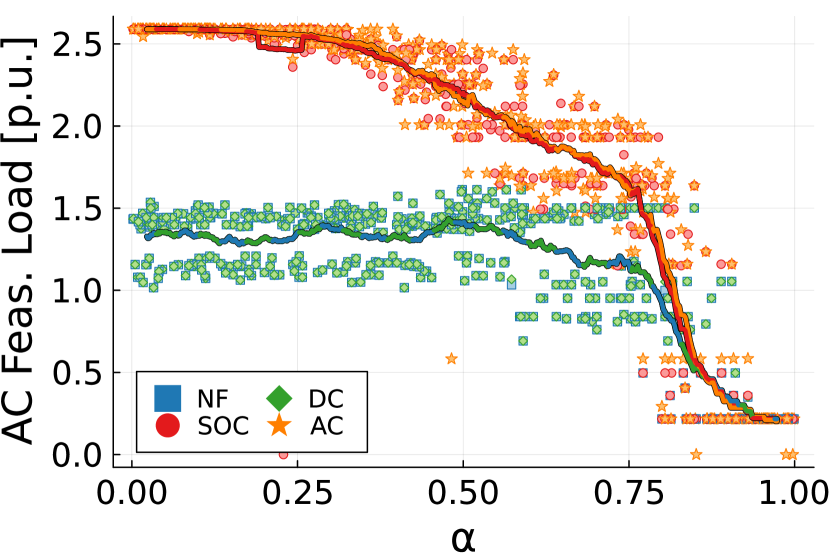
(e)

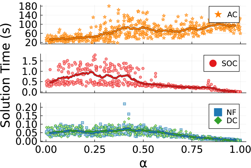
(f)

Figure 1: Case IEEE-14 Fig. 1(a) shows a scatterplot of the OPS objective (Load and Risk) for 500 risk scenarios, solved with four different power flow formulations, as a function of the $\alpha$ parameter. The power delivered to loads is shown in Fig. 1(b) while the wildfire risk is shown in Fig. 1(c). Fig. 1(d) shows the re-calculated objective after an AC-feasible power flow is found. The reduction in load served is shown in Fig. 1(e). Fig. 1(f) shows the solution time for for the OPS problem for each formulation.

We investigate the solution quality and solution time for the normalized OPS problem with different power flow formulations across a range of different power system test cases, wildfire values and choices of the trade-off parameter $\alpha$.

IV-A Case Study Set-Up

1) Software Implementation The OPS problem is implemented using the Julia programming language [27] with the JuMP optimization package [28]. We leverage the DC-OPS implementation in PowerModelsWildfire.jl [3], and extended the package to allow for AC, NF and SOC power flow formulations. These implementations are now publicly available. We use the solvers Gurobi [29] for the NF-, DC- and SOC-OPS and SOC-MLD problems, which are mixed-integer convex (linear or quadratic) programs, Juniper [30] as a heuristic solver for the AC-OPS and AC-MLD problems, which are mixed-integer non-convex (non-linear) problems, and Ipopt [31] for the AC-redispatch problem, which is a continous non-linear problem. We use Distributions.jl [32] to generate random values for our input data (as further described below) and PowerPlots.jl [33] and Plots.jl [34] for visualization.

2) Test systems We use 11 cases from PGLib [35], ranging from 3 to 118 buses. The names of the systems are listed along with the results in Table I.

3) Wildfire data The PGLib test cases do not include any detailed geographical information, and therefore, there is no wildfire power line risk data available. To enable testing on a variety of systems and a large number of scenarios per system, we use randomly generated wildfire risk coefficients $\bm{R}_{ij}$ drawn from a Rayleigh distribution. We chose a Rayleigh distribution because it is a good approximation of wind speed variation [36], and local wildfire risk is closely correlated with wind speed [37].

IV-B Numerical Experiment Set-Up

We generate 500 scenarios for each PGLib test case by sampling wildfire risk coefficients $\bm{R}_{ij}$ for each power line from the Rayleigh distribution. We also sample a $\alpha$ trade-off parameter from a uniform distribution for each scenario, which allows us to study the variation of these scenarios as alpha changes. For each of these scenarios, we solve the NF-, DC-, SOC- and AC-OPS formulations. To maintain a reasonable computational time when solving 500 scenarios, we enforce a 30 minute time limit for each optimization problem and include the results from the time limited scenarios. We do not include results for the AC-OPS on test cases larger than 14-buses and for the SOC-OPS on test cases larger than 39 buses, as a significant number of scenarios (more than 75 of 500) could not be solved within the time limit. For each solution, we record the objective value, load delivered, total power line wildfire risk, and solution time.

After solving the OPS problem, we use our proposed algorithm to recover an AC-feasible solution, and record the resulting load delivered. We also note how frequently the AC-Redispatch problem is infeasible (thus necessitating the solution of an SOC- and possibly AC-MLD problem), and how many scenarios terminate with a trivial AC-feasible solution with 0% load delivery (i.e. how many times AC-MLD reaches the 1 hour time limit in step 3 of the algorithm).

We first present detailed analysis on the IEEE 14 bus case before showing summarized results for the remaining systems.

IV-C IEEE 14 bus case

A collection of results for the IEEE 14-bus case are detailed in Fig 1, where different values on the y-axis are plotted against the range of $\alpha$ values on the x-axis. Individual solutions (corresponding to a set of risk coefficients and an $\alpha$ value) are shown as points in the scatter plots. The lines represent rolling averages of the nearest 30 data points to illustrate trends.

IV-C1 Optimization Problem Results

We first discuss the results obtained by solving the OPS. The upper row show objective value in Fig. 1(a) (right), as well as the resulting load delivered and wildfire risk in Fig. 1(b) and Fig. 1(c), respectively. We first observe from Fig. 1(a) that all power flow formulations find solutions with objective values in a similar range. However, the AC- and SOC-OPS solutions appear to have a slightly lower total objective value than the DC- and NF-OPS solutions. A closer look at Fig. 1(b) and 1(c), explain why. At higher $\alpha$ values $\!>\!\!0.25$, the AC- and SOC-OPS solutions serve slightly less load while the power line risk is comparable. At low $\alpha$ values $\!<\!0.25$, the AC- and SOC-OPS solutions have higher power line risk (i.e. turn off fewer lines) than the DC- and NF-OPS solutions, while serving a similar amount of low. This indicates that to serve a given amount of load, the solutions obtained with AC- and SOC-power flow require a larger number of lines to be energized, thus finding solutions with a higher wildfire risk.

IV-C2 AC-Feasible Load Delivery

Next, we investigate how the load delivery changes after we recover an AC-feasible load delivery solution. The results are shown in Fig. 1(d) and 1(e), which shows the re-calculated objective value and AC-feasible load delivery. By comparing the AC-feasible load delivery in Fig. 1(e) with the load delivery predicted by the optimization solution in Fig. 1(b), we observe that the load delivery achieved with the NF and DC solutions is significantly reduced for $\alpha\!<\!0.85$. The load delivery remains largely the same for the SOC solution across all $\alpha$ values (and the AC solution is already AC feasible). As a result, the objective values of the NF and DC-OPS solutions are significantly reduced, as seen in Fig. 1(d). This indicates that while the NF-, DC-OPS solutions initially produced similar (or even slightly better) objective values, the de-energization decisions were significantly different due to inaccuracies in the NF and DC power flow formulations. As a result, the NF- and DC-OPS solutions only deliver half as much load as the AC and SOC solutions once we recover an AC-feasible solution. This demonstrates that using a more detailed power flow model significantly improves the results.

IV-C3 Solution time

Finally, Fig. 1(f) shows the solution time needed to obtain the solution for each instance. Note that we plot the different problems on three separate scales. We observe that the NF- and DC-OPS problems have similar solution times, while the SOC-OPS take an order of magnitude, i.e., 10x times longer to solve. The AC-OPS is slowest, taking 1000 times longer to solve than the DC and NF solutions. Interestingly, the NF, DC, and SOC formulations are most challenging to solve when $\alpha\!<\!0.5$ where solutions have little load shed and moderate risk reduction. The solution time reduces significantly as $\alpha\rightarrow 1$ where the solution is total de-energization. The trend is not the same for the AC-OPS problem, where the solution time increases as $\alpha\rightarrow 1$.

IV-D PGLib Test Cases

TABLE I: Average OPS objective, AC-feasible objective, and difference

	NF			DC			SOC			AC
Case	Obj.	AC-Feas. Obj.	Diff.	Obj.	AC-Feas. Obj.	Diff.	Obj.	AC-Feas. Obj.	Diff.	Obj.
LMBD 3 Bus	.400561	.363438	.037122	.400561	.363438	.037122	.409230	.405637	.003593	.402468
PJM 5 Bus	.409065	.395903	.013162	.409065	.395903	.013162	.408966	.396111	.012855	.364452
IEEE 14 Bus	.392149	.176974	.215175	.392149	.176992	.215157	.383051	.379996	.003056	.378959
IEEE RTS 24 Bus∗	.377444	.330579	.046866	.377444	.329197	.048247	.370036	.364553	.005483	–
AS 30 Bus	.387029	.316088	.070941	.387029	.316871	.070158	.383347	.380347	.003000	–
IEEE 30 Bus	.353597	.178446	.175150	.353597	.178591	.175006	.346988	.343743	.003245	–
EPRI 39 Bus∗	.366469	.330823	.035646	.366469	.330868	.035602	.362923	.349426	.013497	–
IEEE 57 Bus	.432631	.385885	.046746	.432631	.385860	.046771	–	–	–	–
IEEE RTS 73 Bus†	.391619	–	–	.391620	–	–	–	–	–	–
PEGASE 89 Bus	.641133	.450514	.190619	.641129	.451641	.189488	–	–	–	–
IEEE 118 Bus∗	.347813	.266361	.081453	.347814	.266623	.081191	–	–	–	–

TABLE II: Difference of AC-feasible Objectives

Case	DC-NF	SOC-DC	AC-DC	SOC-AC
LMBD 3 Bus	0.0	.042199	.039030	.003169
PJM 5 Bus	0.0	.000208	-.031451	.031660
IEEE 14 Bus	.000018	.203003	.201967	.001037
IEEE RTS 24 Bus∗	-.001381	.035356	–	–
AS 30 Bus	.000783	.063476	–	–
IEEE 30 Bus	.000145	.165152	–	–
EPRI 39 Bus∗	.000044	.018559	–	–
IEEE 57 Bus	-.000025	–	–	–
IEEE RTS 73 Bus†	–	–	–	–
PEGASE 89 Bus	.001128	–	–	–
IEEE 118 Bus∗	.000262	–	–	–

TABLE III: Infeasible AC-Redis. and AC-MLD Scenarios

	AC Redis. Infeasible			AC MLD Time Out
Case	NF	DC	SOC	NF	DC	SOC
LMBD 3 Bus	0	0	0	0	0	0
PJM 5 Bus	50	50	3	0	0	0
IEEE 14 Bus	0	0	0	0	0	0
IEEE RTS 24 Bus	196	196	12	1	1	1
AS 30 Bus	29	29	0	0	0	0
IEEE 30 Bus	0	0	0	0	0	0
EPRI 39 Bus	349	349	39	17	16	8
IEEE 57 Bus	0	0	–	0	0	–
IEEE RTS 73 Bus	330	330	–	–	–	–
PEGASE 89 Bus	1	1	–	0	0	–
IEEE 118 Bus	12	11	–	9	7	–

We next show summary results for each of the PGLib test cases. Table I reports the summary metrics of solving the 500 scenarios on each of the 11 cases from PGLib using all formulations of the OPS problem. For each network and formulation, we show the average objective value, the objective value after finding an AC-feasible power flow, and the difference between the two. Some scenarios are indicated with $(*)$ to show that the AC-feasible recovery process terminated with a time-limit, and the best feasible solution is used. The number of scenarios where the AC-feasible solution is total load-shed are shown in Table III. The IEEE RTS 73 (${\dagger}$) case does not include AC-feasible results because so many scenarios required the AC-MLD that we were unable to solve the scenarios with one week of computation time.

IV-D1 Accuracy of predicted load shed

We first discuss the ability of the power flow formulations in accurately predicting the load shed value, i.e. have a small difference between the optimization objective and the objective after AC-feasibility recovery. For NF-OPS and DC-OPS, the difference between the objective value of the OPS problem and the re-evaluated objective using AC-feasible power flow range from $0.013$ on the PJM 5 bus network, to $0.215$ on IEEE 14 bus network. This indicates that on some networks, DC-OPF and NF-OPF are reasonably accurate on average, but on other networks they can serve less than half the estimated power delivery. SOC-OPS finds solutions that are very close to AC-feasible, with a difference of less than 0.01 on average for most networks.

IV-D2 Quality of solutions

Next, we discuss how good the solutions are by comparing the amount of load shed after recovering an AC-feasible solution. Table III shows the average objective value difference of the formulations, after finding an AC-feasible power flow. We compare the solutions pairwise, with positive values indicating that the formulation listed first performs better. From the results, we first observe that the DC and NF objective values are nearly identical across all cases, with an average difference close to 0. We therefore compare only the DC formulation with the other power flow formulations. The difference between the DC and SOC objective values shows that the DC formulations performs worse that the SOC solution in all cases. Interestingly, the SOC-OPS with AC-feasibility recovery outperforms the AC-OPS problem on all cases, while even the DC-OPS performs better than the AC-OPS on the PJM 5 bus case. This is because the AC-OPS finds locally optimal solutions when using the Juniper solver.

IV-D3 Difficulty of recovering an AC-Feasible solution

We next discuss the challenges involved with recovering AC-Feasible solutions. Table III reports how many scenarios for each case were infeasible with AC-Redispatch (thus requiring solving the expensive SOC- or AC-MLD problem to recover an AC-feasible power flow) and the number of scenarios where our algorithm terminates without finding an optimal solution (i.e. where the AC-MLD terminates with a time-out). We observe that the NF and DC formulations have many solutions that are AC infeasible, with some networks having close to 70% of scenarios requiring the solution of the MLD problem. However, the DC and NF formulations have only a few scenarios where the AC-MLD reaches the allocated solution time without finding an optimal solution. The SOC formulation has only a few cases where the MLD problem was required to find an AC-feasible power flow, and even fewer where the MLD problem times out.

To identify the cause of AC-infeasibility for the DC- and NF-OPS solutions, we solved the AC-Redispatch problem several times while relaxing a subset of the constraints. For the 39-bus network, lowering the minimum reactive power limit of the generators reduced the number of AC infeasible scenarios, while reducing the the bus minimum voltage had the same effect for the 24-bus, 30-bus, and 73-bus cases. This indicates that the lack of reactive power modeling of the DC and NF formulations is a key factor in the low-quality solutions.

IV-D4 Solution times

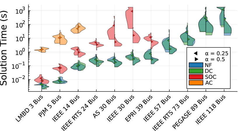
Figure 2: OPS Solve Speed: Distribution of solution time for the PGLib cases at $\alpha$=0.25 and $\alpha$=0.5. The triangles denote the mean value.

Finally, we discuss the solution time. As seen for the IEEE 14 bus system, the solve time can vary greatly depending on the trade-off parameter $\alpha$ and the risk coefficients $\bm{R}_{ij}$. To evaluate solution speed for the PGLib test cases, we solve 50 scenarios at $\alpha=0.25$ and $\alpha=0.5$. We again use a solution time limit of 30 minutes.

Fig. 2 shows the distribution of solution times for different OPS formulations, with a logarithmic y-axis. The results show that solution times for NF- and DC-OPS are generally similar and at least an order of magnitude lower than for SOC-OPS and several orders of magnitude lower than for the AC-OPS, validating the results from the IEEE 14 bus system. We also see that the solution times tend to increase as the systems get bigger, making AC- and SOC-OPS too time consuming for the larger test cases. The difference in solve time when $\alpha\!\!=\!\!0.25$ and $\alpha\!\!=\!\!0.5$ becomes significant in scenarios with more than 24 buses, with $\alpha\!\!=\!\!0.25$ leading to more time consuming problems.

V Conclusion

In this paper, we evaluate the trade-off in solution quality and solution time when modeling the OPS problem with the NF, DC, SOC and AC power flow formulations. To assess the solution quality for the NF, DC and SOC solutions, we devise an algorithm to find AC-feasible solution given the de-energization decisions from the respective OPS problems.

We find that solving the OPS problem with the linear NF and DC power flow formulations tend to significantly overestimate the amount of load that can be served in a given network configuration, thus resulting in solutions with high levels of load shed once the de-energization solutions are checked for AC feasibility. Our analysis indicates that this is likely due to lack of modeling of reactive power and voltage constraints. In comparison, the SOC-based OPS problems tend to more accurately assess the level of load shed, leading to better de-energization decisions. In our case study, SOC-OPS solutions even outperforms the AC-OPS solutions, because the AC-OPS gets stuck at locally optimal solutions.

In terms of solution time, NF and DC based formulations are orders of magnitude faster than SOC and AC power flow. However, the NF- and DC-OPS solutions often required solving the computationally expensive SOC- or AC-MLD problems to recover an AC-feasible solution, which reduces their computational advantage.

Overall, results indicate that current solver technology forces us to pick between low solution quality with DC or NF power flow, or long solution time with SOC or AC power flow. Future work is needed to devise algorithms that can produce high quality solution in reasonable computational time.

References

- [1] H.-O. Pörtner, D. C. Roberts, E. S. Poloczanska et al., “Ipcc, 2022: Summary for policymakers,” 2022.
- [2] “Pacific gas and electric company public safety power shutoff (psps) report to the cpuc october 23-25, 2019 de-energization event,” Pacific Gas & Electric. [Online]. Available: https://tinyurl.com/2s3uzxau
- [3] N. Rhodes, L. Ntaimo, and L. Roald, “Balancing wildfire risk and power outages through optimized power shut-offs,” IEEE Trans. on Power Syst., vol. 36, no. 4, pp. 3118–3128, 2020.
- [4] A. Kody, R. Piansky, and D. K. Molzahn, “Optimizing transmission infrastructure investments to support line de-energization for mitigating wildfire ignition risk,” arXiv preprint arXiv:2203.10176, 2022.
- [5] A. Astudillo, B. Cui, and A. S. Zamzam, “Managing power systems-induced wildfire risks using optimal scheduled shutoffs,” National Renewable Energy Lab, Golden, CO (United States), Tech. Rep., 2022.
- [6] W. Yang, S. N. Sparrow, M. Ashtine et al., “Resilient by design: Preventing wildfires and blackouts with microgrids,” Applied Energy, vol. 313, p. 118793, 2022.
- [7] R. Hanna, “Optimal investment in microgrids to mitigate power outages from public safety power shutoffs,” in 2021 IEEE Power & Energy Society General Meeting (PESGM). IEEE, 2021, pp. 1–5.
- [8] S. Taylor and L. A. Roald, “A framework for risk assessment and optimal line upgrade selection to mitigate wildfire risk,” 2022 Power Syst. Comput. Conf.
- [9] A. Z. Bertoletti and J. C. do Prado, “Transmission system expansion planning under wildfire risk,” in 2022 North Am. Power Symp.
- [10] R. Bayani and S. D. Manshadi, “Resilient expansion planning of electricity grid under prolonged wildfire risk,” IEEE Trans. on Smart Grid, 2023.
- [11] K. Baker, “Solutions of dc opf are never ac feasible,” in Proc. of the Twelfth ACM Int. Conf. on Future Energy Syst., 2021, pp. 264–268.
- [12] W. Hong, B. Wang, M. Yao et al., “Data-driven power system optimal decision making strategy underwildfire events,” Lawrence Livermore National Lab, Tech. Rep., 2022.
- [13] K. W. Hedman, S. S. Oren, and R. P. O’Neill, “A review of transmission switching and network topology optimization,” in 2011 IEEE power and energy society general meeting. IEEE, 2011, pp. 1–7.
- [14] M. Marwali and S. Shahidehpour, “Integrated generation and transmission maintenance scheduling with network constraints,” in Proc. of the 20th Int. Conf. on Power Ind. Comput. Appl. IEEE, 1997, pp. 37–43.
- [15] S. Lumbreras and A. Ramos, “The new challenges to transmission expansion planning. survey of recent practice and literature review,” Electr. Power Syst. Res., vol. 134, pp. 19–29, 2016.
- [16] C. Barrows, S. Blumsack, and P. Hines, “Correcting optimal transmission switching for ac power flows,” in 2014 47th Hawaii Int. Conf. Syst Sci. IEEE, 2014, pp. 2374–2379.
- [17] Y. Bai, H. Zhong, Q. Xia, and C. Kang, “A two-level approach to ac optimal transmission switching with an accelerating technique,” IEEE Trans. on Power Syst., vol. 32, no. 2, pp. 1616–1625, 2016.
- [18] C. Crozier, K. Baker, and B. Toomey, “Feasible region-based heuristics for optimal transmission switching,” Sustainable Energy, Grids and Networks, vol. 30, p. 100628, 2022.
- [19] E. S. Johnson, S. Ahmed, S. S. Dey, and J.-P. Watson, “A k-nearest neighbor heuristic for real-time dc optimal transmission switching,” arXiv preprint arXiv:2003.10565, 2020.
- [20] F. Capitanescu and L. Wehenkel, “An ac opf-based heuristic algorithm for optimal transmission switching,” in 2014 Power Syst. Comput. Conf.
- [21] C. Coffrin, R. Bent, B. Tasseff et al., “Relaxations of ac maximal load delivery for severe contingency analysis,” IEEE Trans. on Power Syst., vol. 34, no. 2, pp. 1450–1458, March 2019.
- [22] N. Rhodes, D. M. Fobes, C. Coffrin, and L. Roald, “Powermodelsrestoration. jl: An open-source framework for exploring power network restoration algorithms,” in 2021 Power Syst. Comput. Conf.
- [23] N. Rhodes and L. Roald, “The role of distributed energy resources in distribution system restoration,” 2022 Hawaii Int. Conf. Syst Sci., 2022.
- [24] N. Rhodes, C. Coffrin, and L. Roald, “Security constrained optimal power shutoff,” arXiv preprint arXiv:2304.13778, 2023.
- [25] R. A. Jabr, “Radial distribution load flow using conic programming,” IEEE Trans. on Power Syst., vol. 21, no. 3, pp. 1458–1459, 2006.
- [26] C. Coffrin, H. Hijazi, and P. Van Hentenryck, “Network flow and copper plate relaxations for ac transmission systems,” in 2016 Power Systems Computation Conference (PSCC). IEEE, 2016, pp. 1–8.
- [27] J. Bezanson, A. Edelman, S. Karpinski, and V. Shah, “Julia: A fresh approach to numerical computing,” SIAM Rev., vol. 59, no. 1, pp. 65–98, 2017. [Online]. Available: https://doi.org/10.1137/141000671
- [28] I. Dunning, J. Huchette, and M. Lubin, “Jump: A modeling language for mathematical optimization,” SIAM Rev., vol. 59, pp. 295–320, 2017.
- [29] Gurobi Optimization, Inc., “Gurobi optimizer reference manual,” Published online at http://www.gurobi.com, 2014.
- [30] O. Kröger, C. Coffrin, H. Hijazi, and H. Nagarajan, “Juniper: An open-source nonlinear branch-and-bound solver in julia,” in Integration of Constraint Programming, Artificial Intelligence, and Operations Research: 15th Int. Conf., Delft, The Netherlands, June 26–29, 2018, Proc. 15. Springer, 2018, pp. 377–386.
- [31] A. Wächter and L. T. Biegler, “On the implementation of an interior-point filter line-search algorithm for large-scale nonlinear programming,” Mathematical programming, vol. 106, pp. 25–57, 2006.
- [32] D. Lin, J. M. White, S. Byrne et al., “JuliaStats/Distributions.jl: a Julia package for probability distributions and associated functions,” Jul. 2019. [Online]. Available: https://doi.org/10.5281/zenodo.2647458
- [33] N. Rhodes, “PowerPlots.jl,” 2023. [Online]. Available: https://github.com/WISPO-POP/PowerPlots.jl
- [34] S. Christ, D. Schwabeneder, C. Rackauckas et al., “Plots.jl – a user extendable plotting api for the julia programming language,” J. of Open Research Software, 2023.
- [35] PGLib Optimal Power Flow Benchmarks, “The ieee pes task force on benchmarks for validation of emerging power system algorithms,” Published online at https://github.com/power-grid-lib/pglib-opf, 2021.
- [36] S. Pishgar-Komleh, A. Keyhani, and P. Sefeedpari, “Wind speed and power density analysis based on weibull and rayleigh distributions (a case study: Firouzkooh county of iran),” Renewable and sustainable energy reviews, vol. 42, pp. 313–322, 2015.
- [37] O. Rios, W. Jahn, E. Pastor et al., “Interpolation framework to speed up near-surface wind simulations for data-driven wildfire applications,” Int. J. of Wildland Fire, vol. 27, pp. 257–270, 2018.