ManifoldNeRF: View-dependent Image Feature Supervision
for Few-shot Neural Radiance Fields

Abstract

Novel view synthesis has recently made significant progress with the advent of Neural Radiance Fields (NeRF). DietNeRF is an extension of NeRF that aims to achieve this task from only a few images by introducing a new loss function for unknown viewpoints with no input images. The loss function assumes that a pre-trained feature extractor should output the same feature even if input images are captured at different viewpoints since the images contain the same object. However, while that assumption is ideal, in reality, it is known that as viewpoints continuously change, also feature vectors continuously change. Thus, the assumption can harm training. To avoid this harmful training, we propose ManifoldNeRF, a method for supervising feature vectors at unknown viewpoints using interpolated features from neighboring known viewpoints. Since the method provides appropriate supervision for each unknown viewpoint by the interpolated features, the volume representation is learned better than DietNeRF. Experimental results show that the proposed method performs better than others in a complex scene. We also experimented with several subsets of viewpoints from a set of viewpoints and identified an effective set of viewpoints for real environments. This provided a basic policy of viewpoint patterns for real-world application. The code is available at https://github.com/haganelego/ManifoldNeRF_BMVC2023

Keywords Few-shot NeRF  $\cdot$ Manifold

1 Introduction

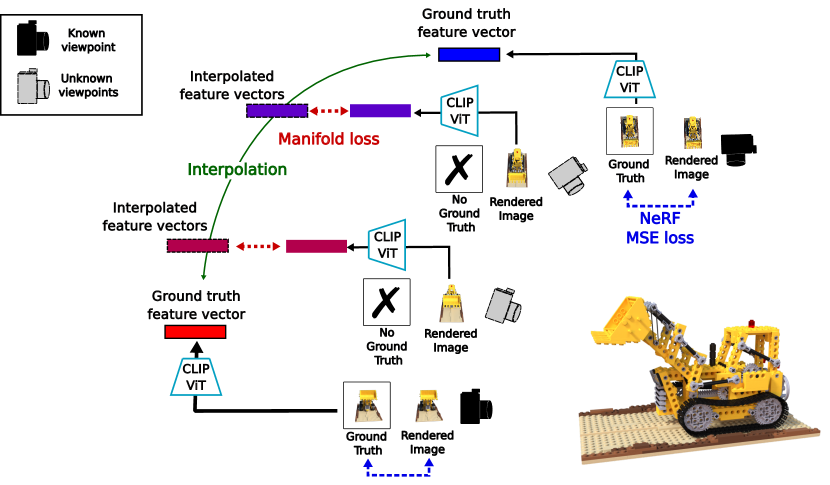
Figure 1: A vanilla NeRF is trained by minimizing the mean squared error (MSE) between a rendered image and the ground truth image at each known viewpoint (NeRF MSE loss). However, when only a few known viewpoints are available, the volumetric scene function cannot be learned, and the rendering of unknown viewpoints does not perform well. If we could give a loss for the outputs from unknown viewpoints, it can be a clue to learning the volumetric scene function even from a few known viewpoints. We propose a new loss for image features at unknown viewpoints supervised by interpolated features from neighboring known viewpoints (Manifold loss), which makes it possible to provide supervision even at unknown viewpoints.

Novel view synthesis is one of the challenging tasks to generate an arbitrary viewpoint image from images at a limited number of viewpoints. NeRF [1] is a method that learns a volumetric scene function from images obtained from a scene using an MSE loss and generates arbitrary viewpoint images by volume rendering [2]. NeRF has been a breakthrough in novel view synthesis, and many methods have been proposed to improve accuracy [3], training speed [4] and application to various fields [5, 6, 7].

Although NeRF is a breakthrough method in novel view synthesis, it still has many limitations. One of the most critical limitations is that it requires a lot of viewpoint images. Recently, the problem of few-shot novel view synthesis has been addressed. DietNeRF [8], one of the few-shot NeRF methods, is based on the assumption that the feature vectors of images of an object at arbitrary viewpoints in the same scene are consistent. In the method, the feature vector at the known viewpoint and feature vectors at arbitrary viewpoints are made closer to each other. Here, the features are obtained from a feature extractor of a pre-trained classifier; we call it “a pre-trained model”. This enables supervision for any viewpoints that are not included in the training dataset, and it demonstrates high performance in the few-shot novel view synthesis task.

However, are the feature vectors obtained by a pre-trained model actually similar for all viewpoints? In an ideal case, the pre-trained model should output identical feature vectors for images of the same object, but in actual situations, feature vectors vary depending on various factors. Among these factors, viewpoint change makes a drastic change in the observed images, which leads to significant changes in the feature vectors. Also, it has been shown that a continuous change in viewpoint causes a continuous change in the feature vectors in the feature space, as introduced in the Parametric Eigenspace method [9]. In the field of pattern recognition, a set of features that varies continuously along some parameters is conventionally called a manifold, and methods such as GAN [10] and VAE [11] acquire the manifold as a latent representation, allowing them to generate continuous changes in facial expressions [12], for example.

Based on the above, we reconsider the assumptions used in DietNeRF. While the feature vectors of images from close viewpoints will certainly be similar, the feature vectors of images from very different viewpoints, such as front and back, are likely to be very different. Therefore, DietNeRF’s training process may constrain the feature vectors, which are inherently very different, to be close to each other; this harms the training of the volumetric scene function. This can be prevented by providing a relaxed assumption that the feature vectors change as the viewpoint changes.

We propose ManifoldNeRF, a novel few-shot NeRF method based on the concept of the manifold. The overview of ManifoldNeRF is shown in Figure 1. In this method, we introduce a novel manifold loss for the training of NeRF. For the calculation, a feature vector at an arbitrary viewpoint is interpolated by the neighboring known viewpoints. The loss is calculated from the interpolated feature vector, named a pseudo ground truth. The difference between the feature vectors extracted from the rendered images at arbitrary viewpoints and the pseudo ground truth is used as the auxiliary loss, as well as the original MSE loss, to train a model. Our contributions are as follows:

• We propose ManifoldNeRF for the few-shot novel view synthesis. We introduce a novel loss function named manifold loss to give supervision for arbitrary viewpoints based on the concept of the Parametric Eigenspace [9].

• We show that by interpolating the feature vectors of neighboring viewpoints, a feature vector that is a good approximation of the ground truth of an interpolated viewpoint can be generated. This enables us to prepare a pseudo ground truth of unknown viewpoints and enables training possible even when the number of known viewpoints is limited.

• We conducted experiments to clarify which viewpoints are important for training a volumetric scene function with a limited number of images. These results establish a basic policy for capturing images for real-world applications.

2 Related works

2.1 Few-shot NeRF

NeRF [1] is a method that embeds a volumetric scene into a volumetric scene function implemented by a multilayer perceptron (MLP), which output color $\mathbf{c}=(r,g,b)^{\top}$ and volume density $\sigma$, 3D location $\mathbf{x}=(x,y,z)^{\top}$ and direction $\mathbf{d}=(\theta,\phi)^{\top}$ as input to MLP. The value of each pixel in an image is calculated by differentiable rendering that enables backpropagation. The loss function is the MSE loss which is commonly used in image reconstruction tasks such as an autoencoder [13].

One drawback of vanilla NeRF is that it requires a lot of images for training. To address this problem, various approaches have been proposed, such as using feature vectors obtained from pre-training models [8, 14, 15, 16], optimization for depth using sparse 3D points [17] and reducing artifact generation by constraining each point on the ray [18, 19].

DietNeRF: In addition to the MSE loss of the vanilla NeRF, DietNeRF introduces a semantic consistency loss to enable training with few images. The loss provides a constraint to force the feature vector obtained from an image at a randomly sampled known viewpoint and the feature vector of a rendered image at an arbitrary viewpoint to be closer. In the method, a pre-trained vision transformer [20] of CLIP [21], which we call it “CLIP-ViT”, is used as a feature extractor. Equation 1 show the semantic consistency loss $\mathcal{L}_{\text{SC}}$ between feature vectors $\mathbf{v}_{k},\mathbf{v}_{u}$ of known and unknown viewpoint is measured by cosine similarity, where $\lambda$ is a scaling factor.

$$\mathcal{L}_{\text{SC}}(\mathbf{v}_{k},\mathbf{v}_{u})=\lambda(1-\mathbf{v}_{k}^{\top}\mathbf{v}_{u}),$$ (1)

Experiments conducted on DietNeRF have shown that the semantic consistency loss is effective when the number of pixels selected is 15%$\sim$20% of the total number of pixels. This method can be trained from a one-shot image and is currently one of the most effective few-shot NeRF methods.

In the proposed method, we select an unknown viewpoint from the neighborhood of the known viewpoints, and we interpolate the feature vector of a viewpoint from the feature vectors of the known viewpoints to obtain pseudo ground truth, aiming to give richer supervision than DietNeRF.

2.2 Manifold

When a camera pose relative to an object changes smoothly, the observed image will also change smoothly. Hence, we can assume that the feature vector extracted from the observed image also changes smoothly according to the camera motion. Based on this assumption, the Parametric Eigenspace method, proposed by Murase et al. [9], interpolates feature vectors at intermediate camera views from two adjacent existing camera views. On the basis of the key concept, the Parametric Eigenspace can model a 3D object using a few images. The method uses a low-dimensional eigenspace calculated by the principal component analysis (PCA) as a feature space and interpolates intermediate image features in the feature space. Here, since a camera pose has six degrees of freedom, the feature vectors are mapped on a 6D hyperplane in the Eigenspace according to the camera parameter. On the hyperplane, feature vectors at similar viewpoints are mapped onto similar points and can be used for interpolation, while calculation using two points far from each other is meaningless. Traditionally, this hyperplane is called a manifold in this field.

Ninomiya et al. [22] have extended the concept of the Parametric Eigenspace; they propose the deep manifold embedding that finds a low-dimensional feature space using deep Learning. The method can find more suitable feature spaces for object pose estimation than PCA. Kawanishi et al. [23] have proposed to use this concept for the latent space of GANs. The method samples a latent variable from a distribution on the manifold corresponding to the camera pose; it makes GANs able to generate an image from a specific viewpoint intuitively. The concept, the Deep Manifold Embedding, has been used in various applications [12, 24, 25] to find a feature space that can model the target with variations.

In this study, we borrow the concept from the Parametric Eigenspace and the Deep Manifold Embedding; we aim to interpolate feature vectors at unknown viewpoints from feature vectors at adjacent known viewpoints to calculate an additional loss for the NeRF training.

3 Feature vector difference according to viewpoints

In this section, we show the results of preliminary experiments that investigate the relationship between viewpoints and feature vectors obtained from a pre-trained model. We used images of the LEGO scene from the NeRF synthetic dataset [1].

First, Figure 2 shows a histogram of the cosine similarity scores for all pairs of the 100 images in the training dataset. The lowest cosine similarity score was about 0.5. We presume that pairs with significantly different viewpoints are included in the area where the cosine similarity score is low.

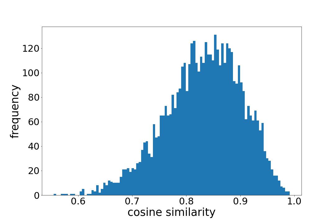
Figure 2: Histogram of cosine similarity scores for all pairs of the 100 images in the LEGO training dataset

Figure 4 shows the comparison of the cosine similarity between the image from the back (target view) of the LEGO and other viewpoints in the training dataset. The cosine similarity score was relatively high when the viewpoint was close to the target view; in contrast, the cosine similarity score was relatively low when the viewpoint differed significantly from the target view. From the above, we expect that the loss function given by DietNeRF would not be so effective when the viewpoints are largely different since it violates the assumption of DietNeRF, while it works when the viewpoints are close to each other.

We further investigated the interpolation of the feature vectors at an unknown viewpoint from two neighboring known viewpoints. The back and side of the LEGO in the training dataset are used as the images at known viewpoints, and a viewpoint between them is selected as an unknown viewpoint. We compared the feature vectors at the three known/unknown viewpoints using cosine similarity. We also compared the groud-truth feature vector at the unknown viewpoint with an interpolated feature from two known viewpoints, which is simply calculated by averaging the two vectors at the known viewpoints, assuming that the unknown viewpoint is exactly in the middle of the two known viewpoints.

The experimental results are shown in Figure 4. The cosine similarity score with the interpolated feature vector was 0.9624, indicating that the interpolated feature vector was closer to the ground-truth feature vector of the image at the unknown viewpoint.

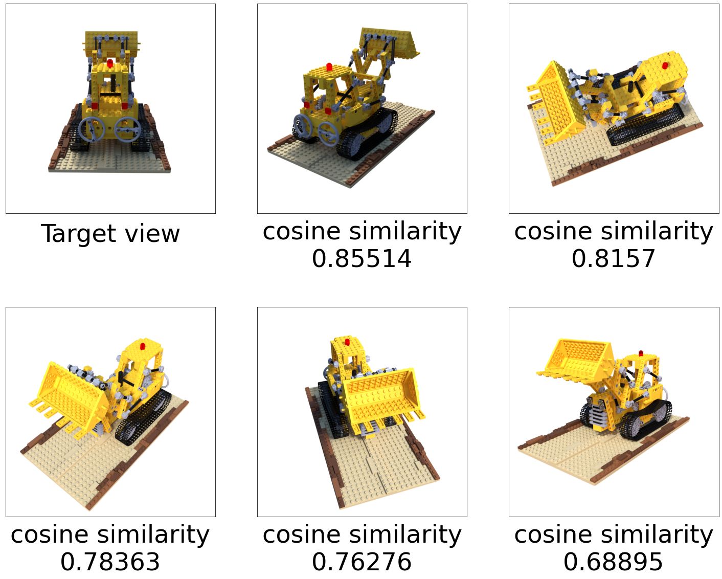
Figure 3: The cosine similarity scores are relatively high for viewpoints that are close to the target view, but the cosine similarity scores are relatively low for viewpoints that are largely far from the target view.

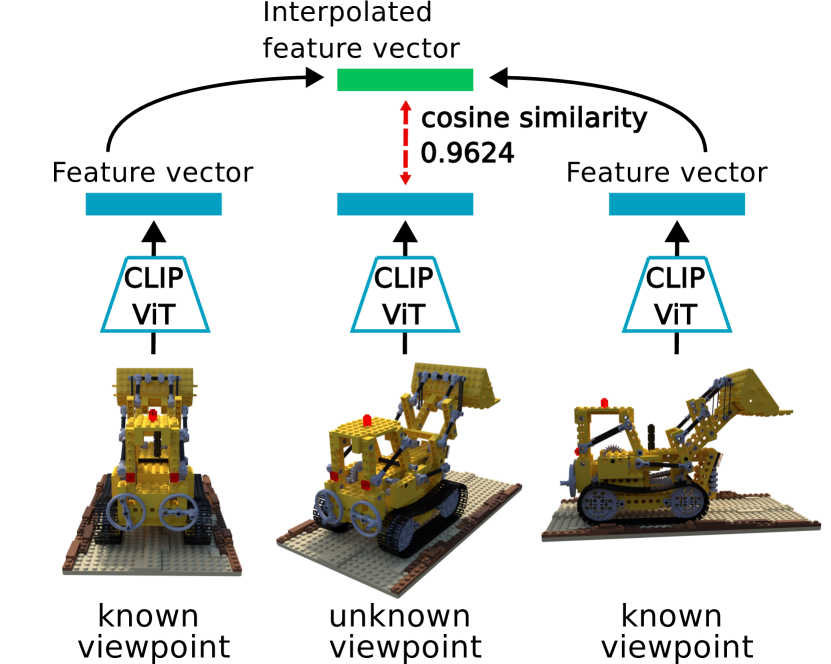
Figure 4: The interpolated feature vectors had a higher cosine similarity score than the cosine similarity scores of the feature vectors obtained from CLIP-ViT for different viewpoints.

4 Proposed method: ManifoldNeRF

Unlike DietNeRF, the proposed method requires an unknown viewpoint to be located between two known viewpoints. Since most 360-degree view scenes are taken from cameras located in a hemisphere from the center of the scene, an arbitrary viewpoint image is generated based on this assumption. Thus, we select an unknown viewpoint $\mathbf{p}_{u}$ by interpolating two known viewpoints $\mathbf{p}_{k,1}$ and $\mathbf{p}_{k,2}$ using spherical linear interpolation (Slerp) [26];

$$\mathbf{p}_{u} =\frac{\sin{(1-s)\theta}}{\sin{\theta}}\mathbf{p}_{k,1}+\frac{\sin{s}\theta}{\sin{\theta}}\mathbf{p}_{k,2},$$ (2)

$$\theta =\arccos{(\mathbf{p}_{k,1},\mathbf{p}_{k,2})},$$ (3)

where $s$ is an interpolation coefficient, which is a random value following a uniform distribution in the range [0, 1]. Each pair of two known viewpoints for choosing unknown viewpoints cannot be too distant since the computation is meaningful only between close points on a manifold; interpolation of feature vectors obtained from the pre-trained model cannot work well between viewpoints that are too distant. Pairs of known viewpoints are sampled if the distance between them is less than a threshold. When interpolating a feature vector $\widehat{\mathbf{v}}_{u}$ between feature vectors $\mathbf{v}_{k,1},\mathbf{v}_{k,2}$ of two viewpoints $\mathbf{p}_{k,1}$ and $\mathbf{p}_{k,2}$ is performed by linear interpolation (Lerp) using the following formula:

$$\widehat{\mathbf{v}}_{u}=(1-s)\mathbf{v}_{k,1}+s\mathbf{v}_{k,2}.$$ (4)

The training process is the same as that of DietNeRF except that we replace the semantic consistency loss with the manifold loss. The manifold loss is the cosine similarity between the feature vector $\mathbf{v}_{u}$ of a rendered image at an arbitrary viewpoint and the feature vector $\widehat{\mathbf{v}}_{u}$ interpolated from known neighboring viewpoints and is calculated by

$$\mathcal{L}_{\text{ML}}(\mathbf{v}_{u},\widehat{\mathbf{v}}_{u})=\lambda(1-\mathbf{v}_{u}^{\top}\widehat{\mathbf{v}}_{u}).$$ (5)

5 Experiments

In this study, all experiments used a 40GB NVIDIA A100. The number of training iterations was 100,000. In Experiments 5.1,  5.2 and  5.3, viewpoint pairs were selected using a threshold of 2.5, while viewpoint pairs were predefined in Experiment 5.4. We used PSNR, SSIM [27], and LPIPS [28] as evaluation metrics. We used the following two public datasets to evaluate the proposed method.

NeRF synthetic dataset: This dataset contains 100 images in each of the 8 scenes by cameras randomly placed in a hemispherical pattern from the center of each object [1]. To evaluate the performance of the proposed method in few-shot scenarios, we randomly selected 8 images as the training dataset for each scene.

DTU MVS dataset: This dataset captures physical object in real environmets and contains 49 images in each of the 128 scenes [29]. We conducted experiments on the 8 scenes and randomly selected 8 images as the training dataset while testing with the remaining 41 images.

5.1 Randomly sampled NeRF synthetic dataset

Table 1 shows the experimental results for each scene. ManifoldNeRF was competitive with DietNeRF and InfoNeRF depending on the scenes, and we could not conclude which method was better in overall performance from this experiment alone.

One of the reasons why the proposed method sometimes performed not well is that the effectiveness of the manifold loss strongly depends on the locations of the known viewpoints. In DietNeRF, the loss can be calculated for any viewpoint in the training process due to the assumption that all feature vectors of arbitrary viewpoints in the same scene should be the same. In contrast, the proposed method can only compute the loss for viewpoints between two neighboring known viewpoints closer than a threshold. Therefore, the proposed method may not perform well depending on the bias of the viewpoints in the training dataset.

Table 1: The results of training 8 randomly selected images in each scene of the NeRF synthetic dataset. The highest score is in bold, and the second highest score is underlined.

PSNR $\uparrow$	LEGO	Chair	Drums	Ficus	Mic	Ship	Materials	Hotdog
NeRF	9.727	18.920	17.032	19.894	12.889	19.535	7.945	10.561
InfoNeRF	9.667	24.964	19.116	20.924	24.233	20.299	20.773	10.752
DietNeRF	22.063	24.722	18.757	21.173	26.383	22.480	20.671	25.746
ManifoldNeRF (ours)	22.171	26.155	18.900	20.489	25.967	23.001	20.819	26.321
NeRF, 100 views	30.336	32.807	25.144	28.174	32.196	28.654	28.459	35.758

5.2 Uniformly sampled NeRF synthetic dataset

Based on the experiments in the previous section, we selected images for training and evaluation to avoid bias. This experiment was conducted in the LEGO scene of NeRF synthetic dataset. We generated 8 viewpoint images from the Blender model that were evenly distributed across the scene, with 4 images for each side and 4 images for the overhead view as shown in Figure 5. The experimental results are shown in Table 2 and Figure 6. These results show that the proposed method achieves better PSNR+7.471, SSIM+0.146, and LPIPS-0.150 than DietNeRF, confirming the superior performance of the proposed method.

In this experiment, the performance of DietNeRF was low compared to the experiment of Sec. 5.1. We consider that this is due to constraints on DietNeRF. As shown in Figure 2, the cosine similarity is varied, and Figure 4 shows that the lowest cosine similarity is 0.68. From the above, the constraints on DietNeRF may bring feature vectors that are very different close together. On the other hand, the proposed method showed high performance when the viewpoints were evenly distributed across the scene. Considering real-world applications, we can control the viewpoints to be taken. Therefore, the viewpoint constraint in the proposed method is not a drawback in real-world applications.

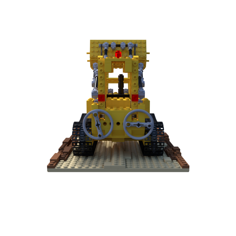
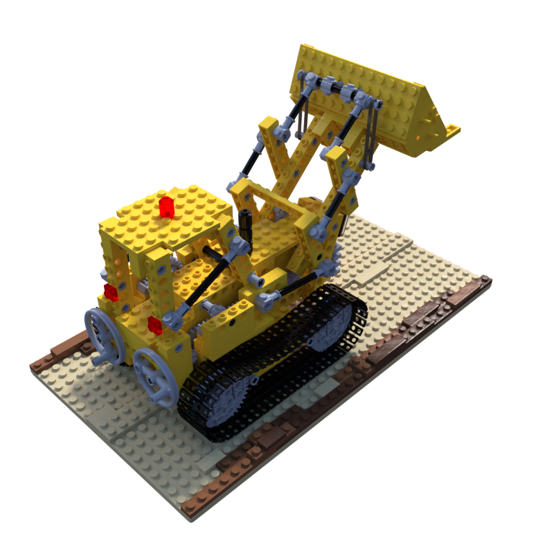
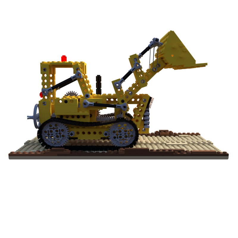
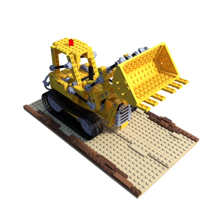
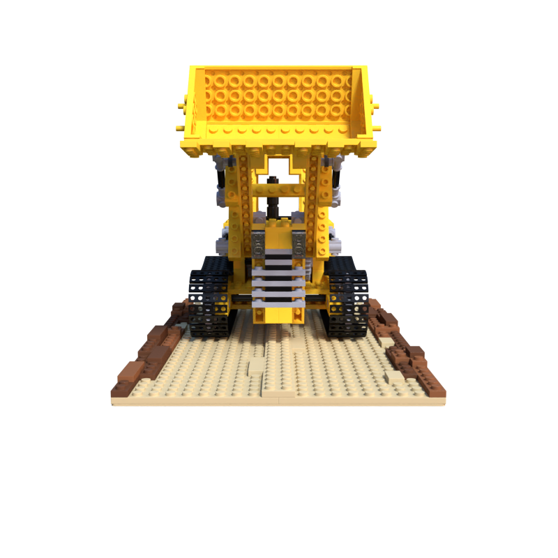
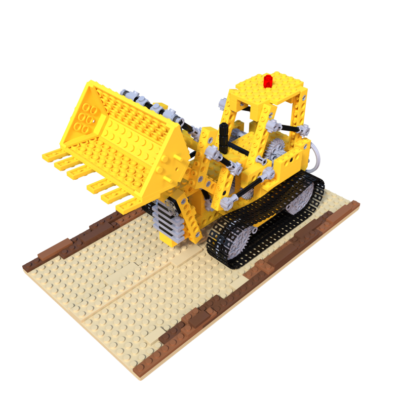
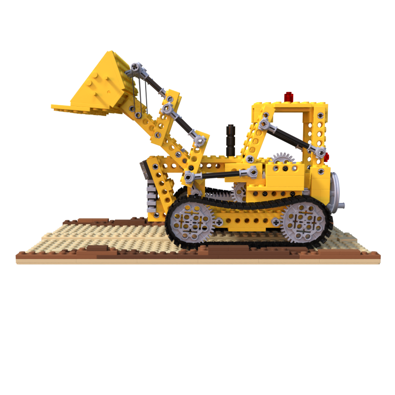
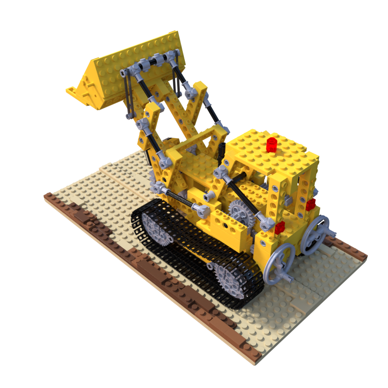
Figure 5: Viewpoint images of the LEGO training dataset for the experiment in Sec. 5.2.

Table 2: The result of training using images at uniformly selected viewpoints from the LEGO scene of the NeRF synthetic dataset. The highest score is in bold.

Method	PSNR $\uparrow$	SSIM $\uparrow$	LPIPS $\downarrow$
DietNeRF	15.233	0.713	0.267
ManifoldNeRF (ours)	22.704	0.859	0.117

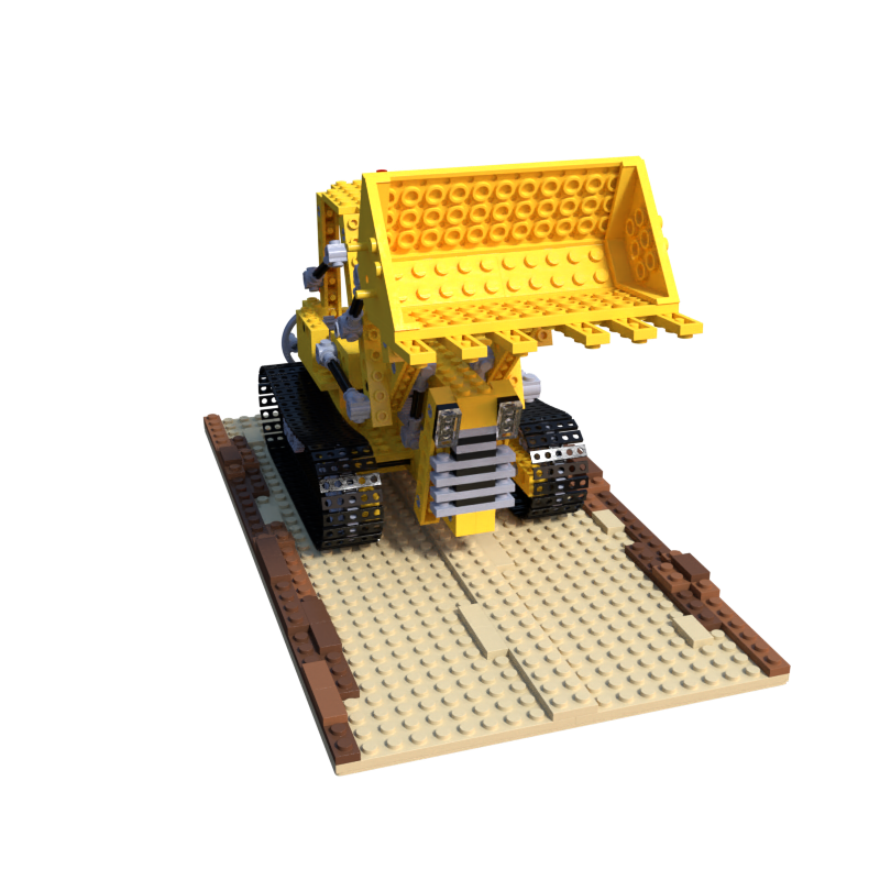
Ground Truth

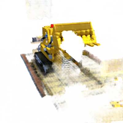
DietNeRF

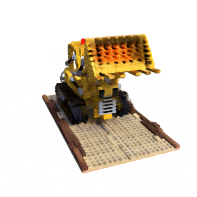
ManifoldNeRF(ours)

Figure 6: Qualitative comparison on the NeRF synthetic dataset for the experiment in Sec. 5.2

5.3 Randomly sampled DTU MVS dataset

Table 3 and Figure 7 shows the experimental result for #65 and #114 scenes. We confirmed that the proposed method achieved the best performance in this experiment with two scenes.

We consider that the high performance of the proposed method in this experiment is due to its constraint, which can be optimized well in complex scenes such as the DTU MVS dataset. The NeRF synthetic dataset is generated from a 3D model in Blender, so there is less noise in the image. On the other hand, datasets taken in real environments are likely to contain disturbance due to background effects and other factors. Therefore, the feature vectors at different viewpoints in the same scene are likely to differ significantly. The constraints of the proposed method generate feature vectors between neighboring viewpoints considering disturbances. From the above, we believe that the proposed method performs well in real environments.

Table 3: The results of training 8 randomly selected images in #65 and #114 scene of the DTU MVS dataset. The highest score is in bold, and the second-highest score is underlined.

#65	PSNR $\uparrow$	SSIM $\uparrow$	LPIPS $\downarrow$
NeRF	11.970	0.481	0.527
InfoNeRF	14.786	0.484	0.431
DietNeRF	20.883	0.698	0.352
ManifoldNeRF (ours)	22.197	0.702	0.302

#114	PSNR $\uparrow$	SSIM $\uparrow$	LPIPS $\downarrow$
NeRF	18.691	0.636	0.396
InfoNeRF	21.382	0.611	0.364
DietNeRF	20.861	0.673	0.337
ManifoldNeRF (ours)	23.202	0.732	0.299

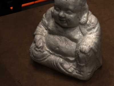
Ground Truth

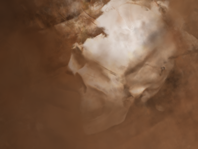
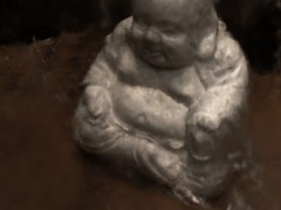
NeRF

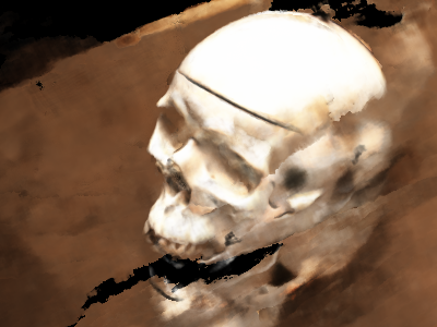
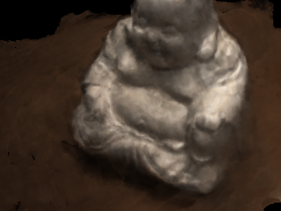
InfoNeRF

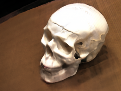
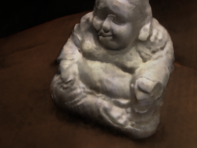
DietNeRF

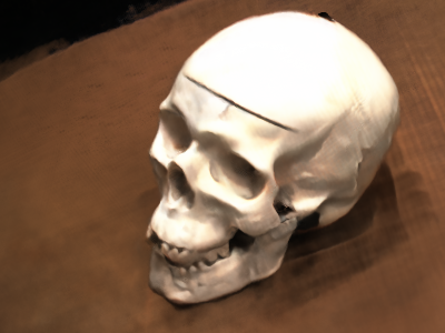
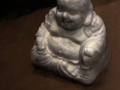
ManifoldNeRF (ours)

Figure 7: Qualitative comparison on the #65(Top) and #114(Bottom) of the MVS DTU dataset for the experiment in Sec 5.3

5.4 Evaluation of viewpoint patterns for real-world application

In this section, we evaluate several viewpoint patterns to see which viewpoints are appropriate for training ManifoldNeRF from images taken in real environments. In this experiment, we used “cheezit”, one of the Yale-CMU-Berkeley object [30], which is used as a common benchmark dataset for object manipulation and object recognition. This object was taken images using a Realsense D435, and the image was center-cropped and background-removed. As shown in Figure 8, each viewpoint pattern was taken from 8 directions around the object: (1) horizontally toward the object, (2) diagonally above the object, and (3) alternate horizontally and diagonally to the object.

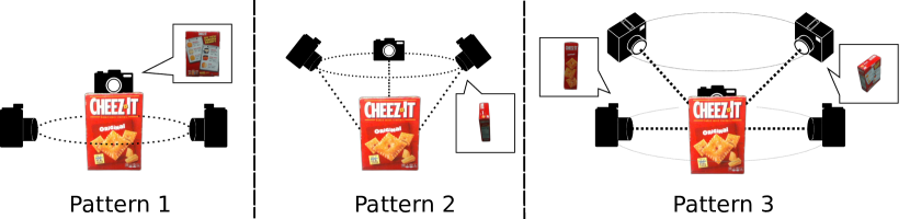
Figure 8: Patterns for taking images for Experiment 5.4

Table 4: Experimental results for each viewpoint pattern. The highest score is in bold, and the second highest score is underlined.

ManifoldNeRF	PSNR $\uparrow$	SSIM $\uparrow$	LPIPS $\downarrow$
Pattern1	17.983	0.849	0.147
Pattern2	21.143	0.871	0.114
Pattern3	23.203	0.899	0.074

Table 4 shows the results of training on each pattern with the proposed method. The proposed method had the best performance for Pattern 3.

The reason why viewpoint Pattern 3 had the best performance in the proposed method is due to the wide range of unknown viewpoints for which feature vector interpolation was possible. In Patterns 1 and 2, we could only interpolate feature vectors horizontally. On the other hand, Pattern 3 could interpolate feature vectors not only horizontally, but also for viewpoints in diagonal directions. Therefore, we expect that, when taking pictures in a real environment, it will be possible to generate a high-quality volume scene with a few viewpoint images by taking pictures from viewpoints from which feature vectors can be interpolated more variously. S between these directions.

6 Conclusion

In this study, we proposed ManifoldNeRF, a new method for few-shot novel view synthesis. On the basis of the assumption that the feature vectors obtained from the pre-trained model also change continuously when the viewpoint of the image changes continuously, the feature vectors at unknown viewpoints nearby known viewpoints can be obtained by interpolation.

Experimental results show that ManifoldNeRF performs well when the known viewpoints are uniformly selected for the scene. In addition, we clarified which viewpoint pattern is better in real environments, and established a basic policy for practical applications.

In future work, we aim to improve performance further and apply the proposed NeRF method to real-world applications using robots.

In this study, we considered that optimization for various unknown viewpoints is important for improving performance, so we employed uniform sampling. Although not addressed in this study, a strategy that focuses sampling near the centre of the two known viewpoints is based on the assumption that the area around the known viewpoints can be trained without using pseudo ground truth. From the above, we believe that the accuracy can be further improved by changing the method of selecting unknown viewpoints.

In real-world environments, robots may encounter unknown objects, which they need to learn by themselves. A large number of object images are required for training, but it is time-consuming for the robot to take a large number of images by its own observation. Using the proposed method, we can obtain a volumetric representation of an unknown object from a few images. From this volumetric representation, we can generate a large data set, which can be used for object recognition and other purposes.

A Experimental details

The proposed method was trained by following a training process shown in Algorithm 1. The hyperparameters in the training process, manifold loss interval $K$ and scaling factor $\lambda$, were set to 10 and 0.1, respectively. These are the same values as used in the official implementation of DietNeRF [8].

Data: Known viewpoints $\mathcal{D}=\{(I,\mathbf{p})\}$, a pre-trained feature extractor $\phi(\cdot)$,

threshold of distance between viewpoints $\epsilon$, manifold loss interval $K$, scaling factor $\lambda$, batch size $|\mathcal{R}|$, learning rate $\eta_{i}$, MSE loss $\mathcal{L}_{\text{MSE}}$, manifold loss $\mathcal{L}_{\text{ML}}$

Result: Trained Neural Radiance Field $f_{\theta}(\cdot,\cdot)$

1 Initialize NeRF $f_{\theta}(\cdot,\cdot)$;

2 Pre-compute feature vectors $\mathcal{V}=\{\mathbf{v}=\phi(I):(I,\mathbf{p})\in\mathcal{D}\}$;

3 Pre-compute pairs of viewpoint $\mathcal{P}=\{(\{\mathbf{p}_{k,1},\mathbf{v}_{k,1}\},\{\mathbf{p}_{k,2},\mathbf{v}_{k,2}\}):(I_{k,1},\mathbf{p}_{k,1}),(I_{k,2},\mathbf{p}_{k,2})\in\mathcal{D},\mathbf{v}_{k,1},\mathbf{v}_{k,2}\in\mathcal{V}\;,if\;|\mathbf{p}_{k,1}-\mathbf{p}_{k,2}|<\epsilon\}$ ;

4 for i from 1 to num_iters do

5       Sample ray batch $\mathcal{R}$, ground-truth colors $\mathbf{C}(\cdot)$;

6       Render rays $\widehat{\mathbf{C}}(\cdot)$;

7       $\mathcal{L}\leftarrow\mathcal{L}_{\text{MSE}}(\mathcal{R},\mathbf{C},\widehat{\mathbf{C}})$;

8       if $i~{}\%~{}K=0$ then

9             Sample pair of viewpoints $(\{\mathbf{p}_{k}^{1},\mathbf{v}_{k,1}\},\{\mathbf{p}_{k,2},\mathbf{v}_{k,2}\})\sim\mathcal{P}$;

10             Compute interpolation coefficient $s$;

11             Compute unknown viewpoint $\widehat{\mathbf{p}}_{u}=SLERP(\mathbf{p}_{k,1},\mathbf{p}_{k,2},s)$;

12             Render image $\widehat{I}$ at viewpoint $\widehat{\mathbf{p}}_{u}$;

13             Compute feature vector of $\widehat{I}$: $\widehat{\mathbf{v}}_{u}=\phi{(\widehat{I})}$;

14             Interpolate feature vector $\mathbf{v}_{u}=LERP(\mathbf{v}_{k,1},\mathbf{v}_{k,2},s)$

15            $\mathcal{L}\leftarrow\mathcal{L}+\mathcal{L}_{\text{ML}}(\mathbf{v}_{u},\widehat{\mathbf{v}}_{u})$;

16            

17       end if

18      Update parameters: $\theta\leftarrow Adam(\theta,\eta_{i},\nabla_{\theta}\mathcal{L})$;

19      

20 end for

Algorithm 1 Training process of ManifoldNeRF

The IDs of the known viewpoints used in the randomly selected experiments from the NeRF synthetic dataset [31] were $[2,16,26,55,73,75,86,93]$, and those used in the DTU MVS dataset were $[0,6,7,23,32,37,39,48]$.

B Analysis of feature vector obtained from pre-trained feature extractor

In this section, we describe experiments conducted to verify the changes in feature vectors with a change in viewpoints. For this experiment, we generated 36 images rendered by rotating the camera position by 10 degrees around an axis of the LEGO scene in the NeRF synthetic dataset. We input these images to the vision encoder of the CLIP to obtain the feature vectors. The obtained feature vectors were projected onto a 2D space using UMAP and visualized in the 2D space to confirm the changes in feature vectors along with continuous changes in viewpoints.

The experimental results are shown in Fig. 9. The feature vectors of adjacent viewpoints are located in the neighborhood, indicating that the feature vectors change continuously as the viewpoints change, as claimed by the Parametric Eigenspace [9].

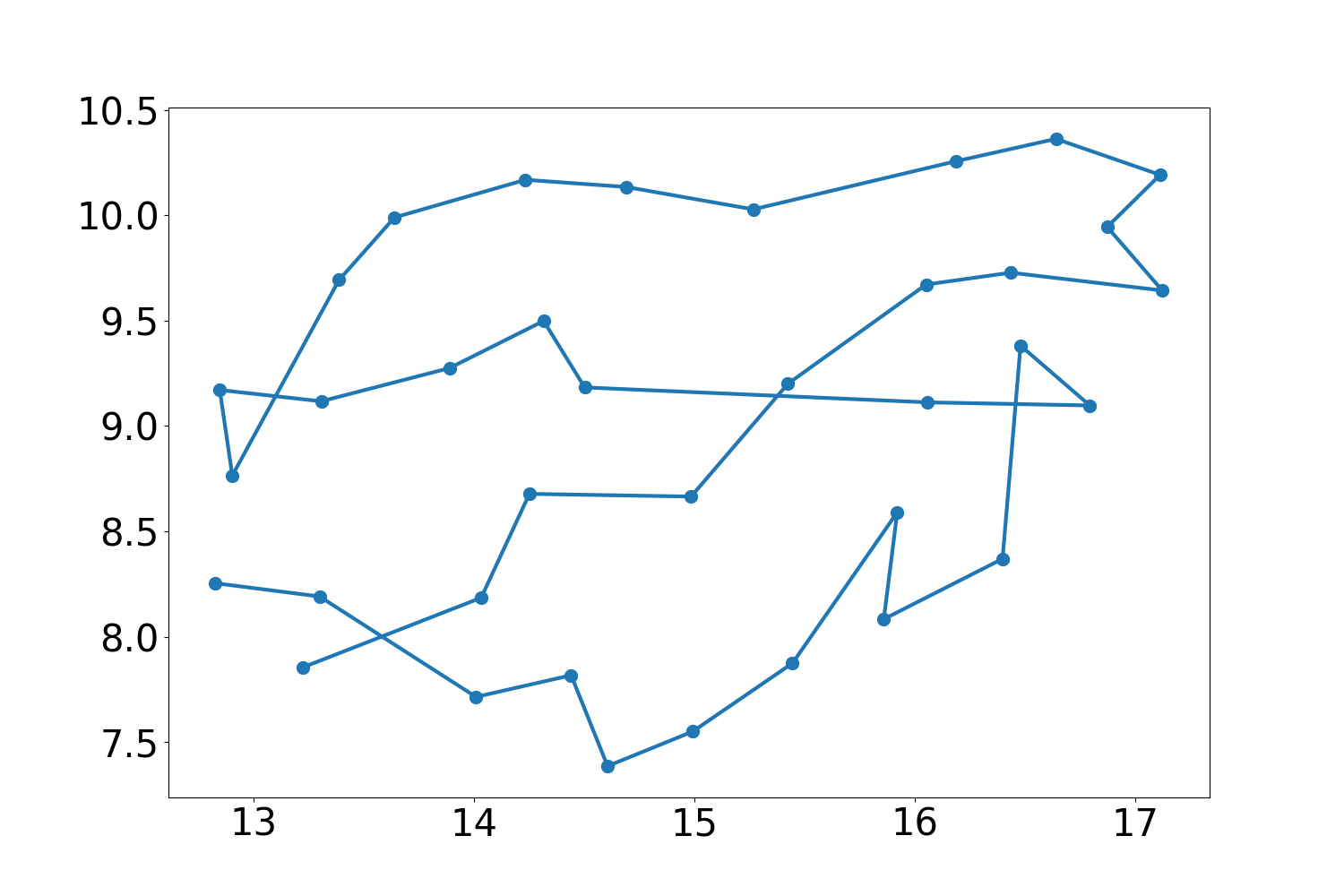
Figure 9: Projected feature vectors extracted with the pre-trained feature extractor into a two-dimensional space using UMAP. The dots in the graph denote the projected feature vectors, and the lines connect the dots corresponding to adjacent viewpoints.

C Performance with different numbers of training data

In the experiments conducted in Sec. 3 of the paper, the feature vectors between viewpoints differing by 90 degrees were calculated to be close to the ground truth. Therefore, we assumed that the performance of the proposed method would be higher when we selected 8 images if we prepared viewpoints that differ by 90 degrees from each other in the horizontal and the diagonal viewpoints.

In this section, we evaluated the change in performance when the number of training data is changed. Table 5 shows the experimental results when we changed the training data for NeRF and ManifoldNeRF to 4, 8, 12, and 16. NeRF perform poorly when the training data is less than 16. However, the performance of ManifoldNeRF increased significantly when the training data was 8 and above.

Table 5: Results of performance change with different number of training data. The training dataset is a LEGO scene from the NeRF synthetic dataset.

NeRF	PSNR $\uparrow$	SSIM $\uparrow$	LPIPS $\downarrow$
4	9.035	0.504	0.468
8	9.727	0.521	0.469
12	10.001	0.552	0.455
16	27.613	0.926	0.065

ManifoldNeRF	PSNR $\uparrow$	SSIM $\uparrow$	LPIPS $\downarrow$
4	9.219	0.526	0.464
8	21.607	0.806	0.174
12	25.215	0.874	0.108
16	25.793	0.884	0.102

D Details of experimental results using the DTU MVS dataset

Table 6 and Fig. 10 show the experimental results for 8 scenes selected from the DTU MVS dataset [29]. ManifoldNeRF performed well in 4 scenes of the 8 scenes. However, in the remaining 4 scenes, the performance was comparable to that of vanilla NeRF. The reason why the proposed method sometimes performed not well is that the performance of ManiofldNeRF is strongly dependent on the location of known viewpoints. In contrast, InfoNeRF [18] performed more stably than the other methods.

Table 6: Results of training 8 randomly selected images in 8 scene of the DTU MVS dataset. The highest score is in bold, and the second-highest score is underlined.

#6	PSNR $\uparrow$	SSIM $\uparrow$	LPIPS $\downarrow$
NeRF	15.550	0.460	0.472
InfoNeRF	13.352	0.397	0.462
DietNeRF	15.210	0.426	0.476
ManifoldNeRF (ours)	16.232	0.508	0.451

#56	PSNR $\uparrow$	SSIM $\uparrow$	LPIPS $\downarrow$
NeRF	21.484	0.621	0.353
InfoNeRF	18.644	0.477	0.474
DietNeRF	19.026	0.538	0.427
ManifoldNeRF (ours)	22.197	0.639	0.367

#65	PSNR $\uparrow$	SSIM $\uparrow$	LPIPS $\downarrow$
NeRF	11.970	0.481	0.527
InfoNeRF	14.786	0.484	0.431
DietNeRF	20.883	0.698	0.352
ManifoldNeRF (ours)	22.197	0.702	0.302

#114	PSNR $\uparrow$	SSIM $\uparrow$	LPIPS $\downarrow$
NeRF	18.691	0.636	0.396
InfoNeRF	21.382	0.611	0.364
DietNeRF	20.861	0.673	0.337
ManifoldNeRF (ours)	23.202	0.732	0.299

#30	PSNR $\uparrow$	SSIM $\uparrow$	LPIPS $\downarrow$
NeRF	8.054	0.491	0.560
InfoNeRF	17.657	0.663	0.254
DietNeRF	6.092	0.298	0.675
ManifoldNeRF (ours)	6.406	0.387	0.633

#41	PSNR $\uparrow$	SSIM $\uparrow$	LPIPS $\downarrow$
NeRF	8.236	0.312	0.636
InfoNeRF	14.681	0.484	0.423
DietNeRF	8.36	0.246	0.636
ManifoldNeRF (ours)	8.963	0.317	0.628

#45	PSNR $\uparrow$	SSIM $\uparrow$	LPIPS $\downarrow$
NeRF	7.558	0.220	0.710
InfoNeRF	10.719	0.422	0.441
DietNeRF	7.097	0.216	0.662
ManifoldNeRF (ours)	7.418	0.181	0.721

#61	PSNR $\uparrow$	SSIM $\uparrow$	LPIPS $\downarrow$
NeRF	7.793	0.236	0.684
InfoNeRF	14.634	0.543	0.395
DietNeRF	11.974	0.463	0.508
ManifoldNeRF (ours)	7.518	0.267	0.679

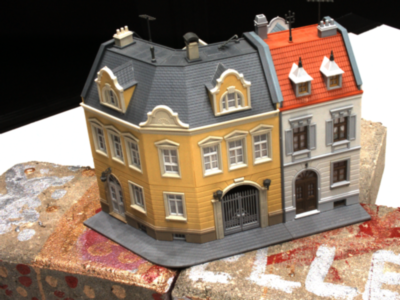
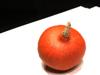
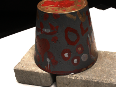
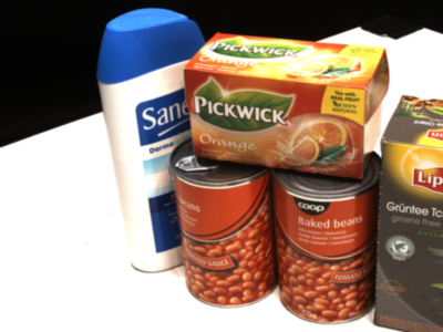
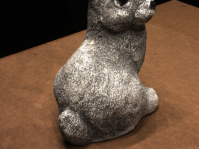
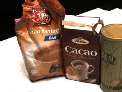
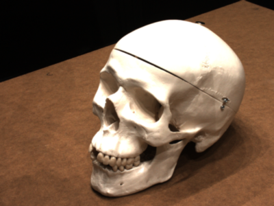
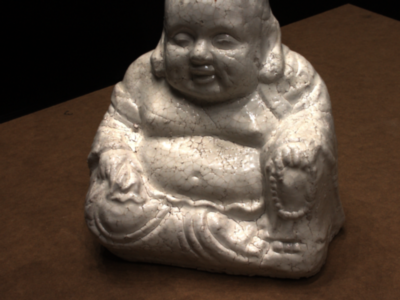
Ground Truth

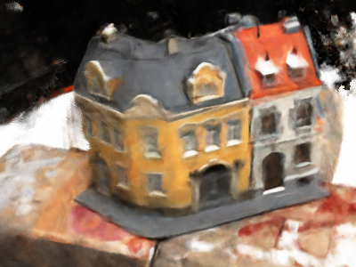
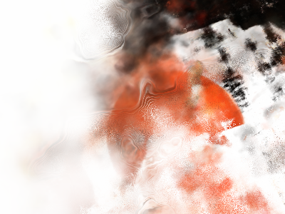
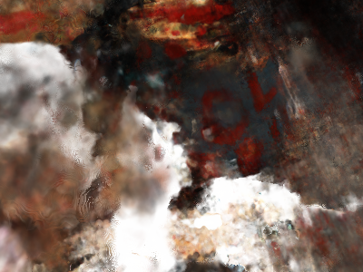
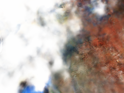
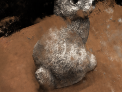
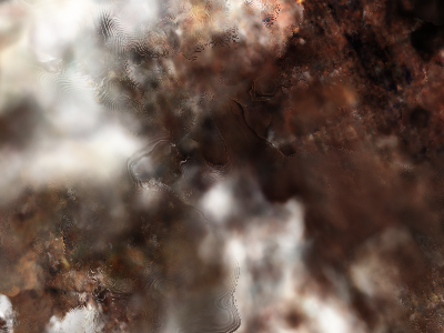
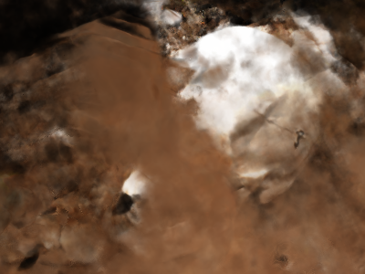
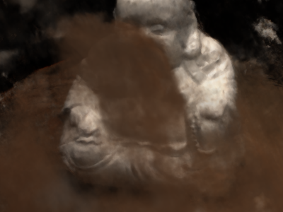
NeRF

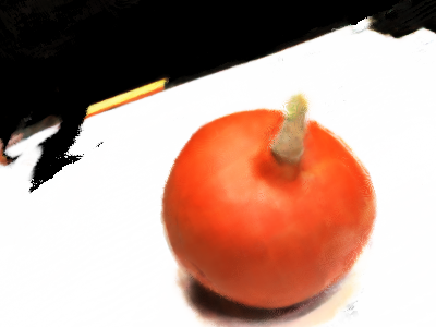
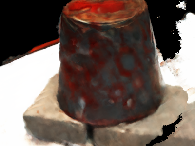
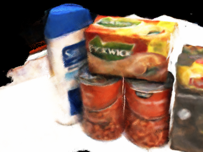
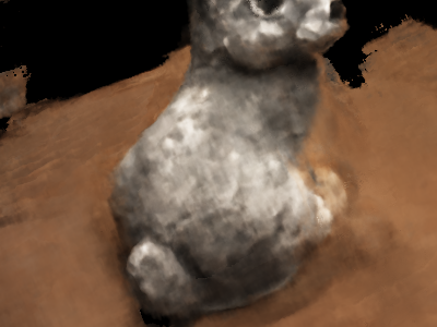
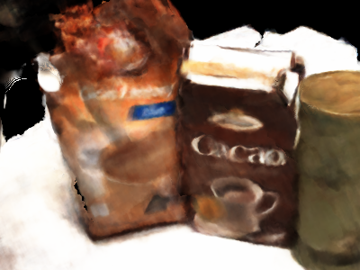
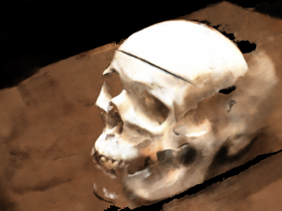
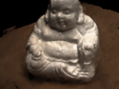
InfoNeRF

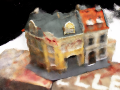
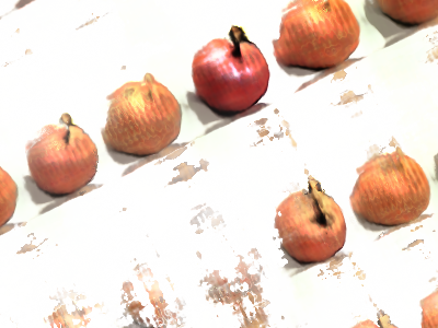
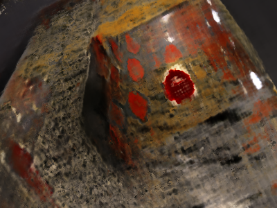
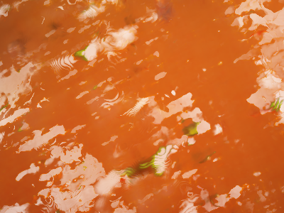
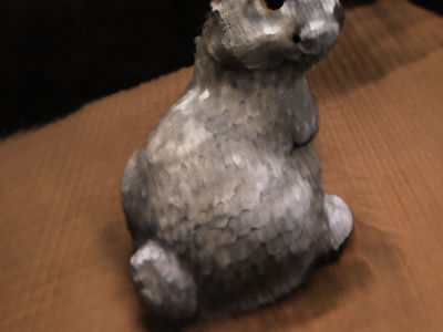
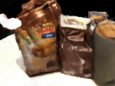
DietNeRF

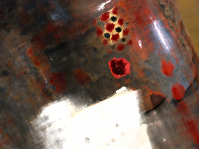
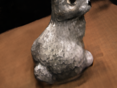
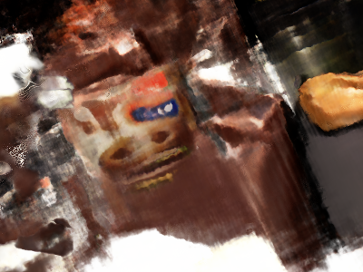
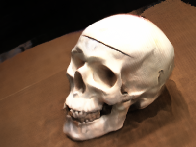
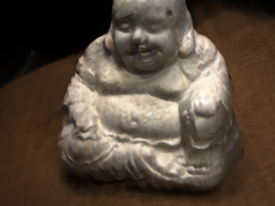
ManifoldNeRF (ours)

Figure 10: Qualitative comparison on 8 scenes of the MVS DTU dataset

Next, Table 7 and Fig. 11 show the results of fine-tuning the model trained with InfoNeRF using ManifoldNeRF. We confirmed the performance improvement by fine-tuning the model trained with InfoNeRF. The reason for the performance improvement is that InfoNeRF applies constraints to each point on the ray, whereas ManifoldNeRF applies constraints to the feature vectors of the image obtained from the viewpoints between neighbouring viewpoints, and the optimization targets are different. From the above, we demonstrate that even when the known viewpoints are random, combining other methods with the proposed method can improve performance.

Table 7: Results of fine-tuning the model trained with InfoNeRF using ManifoldNeRF. The results w/o fine-tuning are the same as for InfoNeRF in Table 6. The highest score is in bold, and the second-highest score is underlined.

#6	PSNR $\uparrow$	SSIM $\uparrow$	LPIPS $\downarrow$
w/o fine-tuning	13.352	0.397	0.462
20k iters	15.157	0.438	0.491
40k iters	15.210	0.448	0.476
60k iters	15.087	0.461	0.458s
80k iters	15.211	0.471	0.458
100k iters	15.398	0.472	0.448

#30	PSNR $\uparrow$	SSIM $\uparrow$	LPIPS $\downarrow$
w/o fine-tuning	17.657	0.663	0.254
20k iters	20.335	0.808	0.197
40k iters	20.412	0.828	0.185
60k iters	20.364	0.839	0.183
80k iters	20.359	0.835	0.180
100k iters	20.285	0.837	0.179

#41	PSNR $\uparrow$	SSIM $\uparrow$	LPIPS $\downarrow$
w/o fine-tuning	14.681	0.484	0.423
20k iters	17.032	0.570	0.443
40k iters	17.111	0.585	0.427
60k iters	16.890	0.582	0.422
80k iters	16.904	0.595	0.411
100k iters	17.031	0.599	0.405

#45	PSNR $\uparrow$	SSIM $\uparrow$	LPIPS $\downarrow$
w/o fine-tuning	10.719	0.422	0.441
20k iters	14.867	0.504	0.412
40k iters	14.882	0.514	0.399
60k iters	14.842	0.520	0.390
80k iters	14.898	0.523	0.389
100k iters	14.903	0.523	0.383

#56	PSNR $\uparrow$	SSIM $\uparrow$	LPIPS $\downarrow$
w/o fine-tuning	18.644	0.477	0.474
20k iters	19.912	0.510	0.472
40k iters	20.130	0.528	0.462
60k iters	19.880	0.532	0.458
80k iters	19.773	0.531	0.453
100k iters	19.902	0.540	0.451

#61	PSNR $\uparrow$	SSIM $\uparrow$	LPIPS $\downarrow$
w/o fine-tuning	14.634	0.543	0.395
20k iters	15.588	0.544	0.437
40k iters	15.926	0.554	0.420
60k iters	15.772	0.563	0.415
80k iters	15.861	0.568	0.409
100k iters	15.799	0.560	0.403

#65	PSNR $\uparrow$	SSIM $\uparrow$	LPIPS $\downarrow$
w/o fine-tuning	14.786	0.484	0.431
20k iters	20.468	0.658	0.369
40k iters	20.615	0.673	0.349
60k iters	20.654	0.687	0.339
80k iters	20.768	0.693	0.334
100k iters	20.821	0.705	0.331

#114	PSNR $\uparrow$	SSIM $\uparrow$	LPIPS $\downarrow$
w/o fine-tuning	21.382	0.611	0.364
20k iters	21.902	0.658	0.372
40k iters	22.092	0.672	0.358
60k iters	21.948	0.677	0.350
80k iters	21.791	0.673	0.350
100k iters	21.696	0.675	0.346

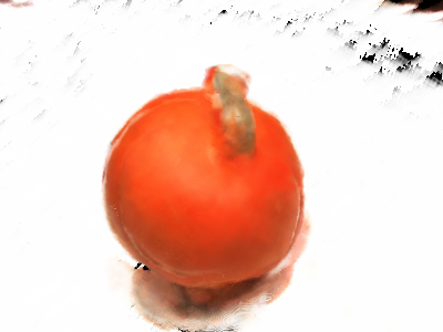
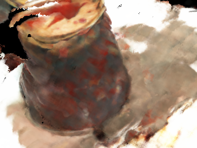
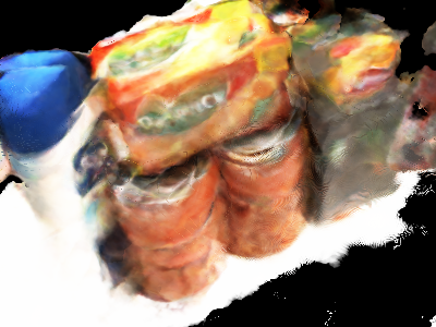
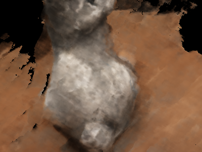
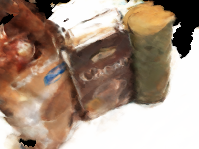
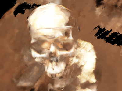
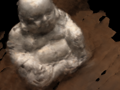
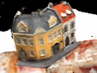
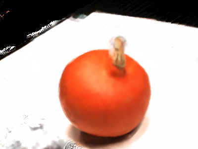
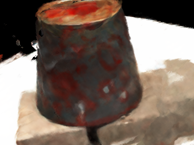
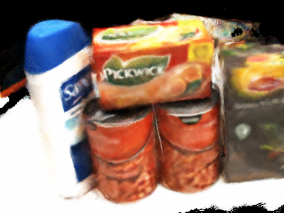
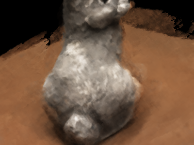
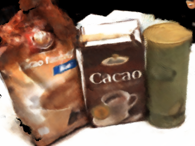
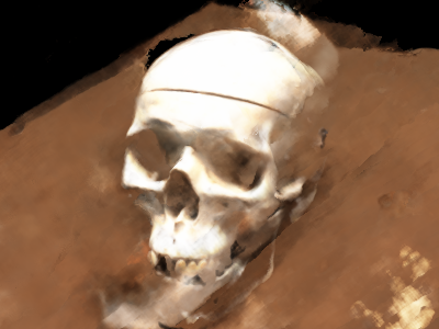
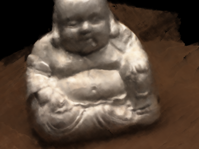
w/o fine-tuning

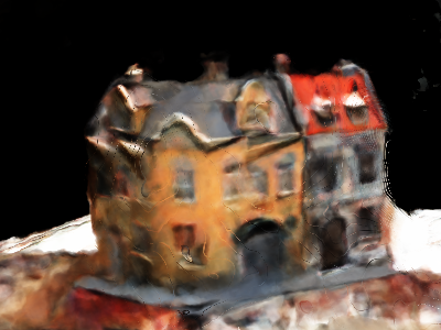
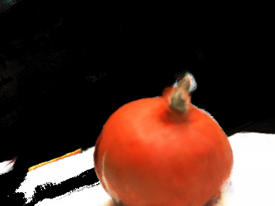
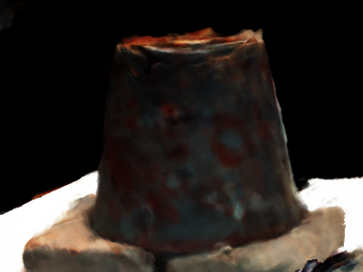
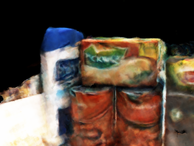
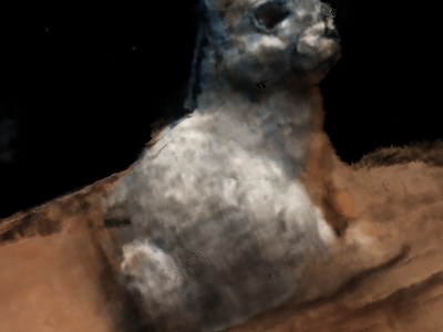
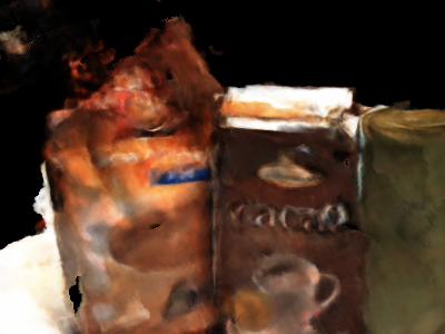
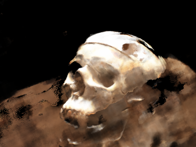
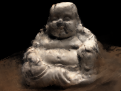
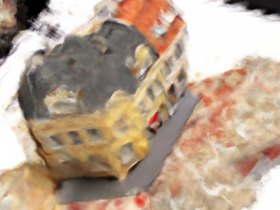
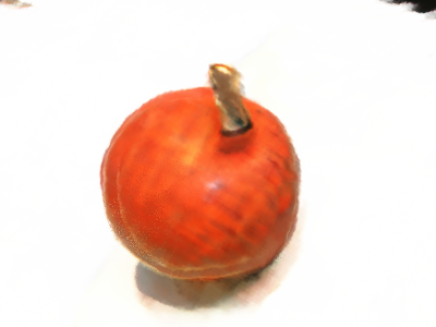
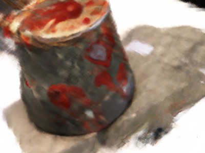
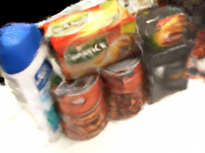
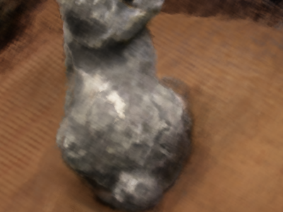
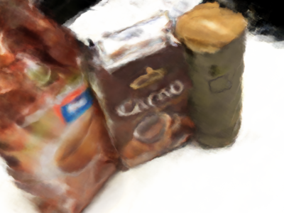
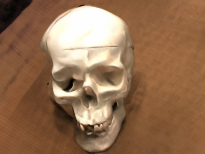
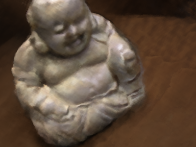
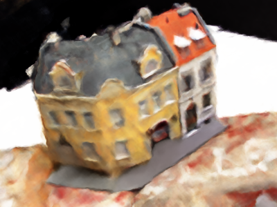
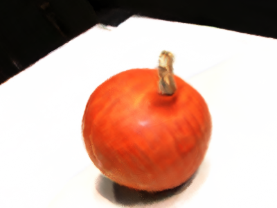
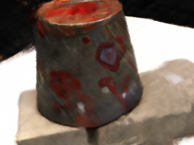
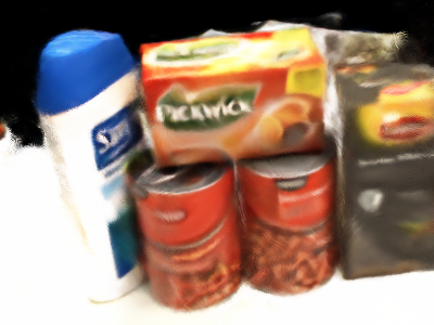
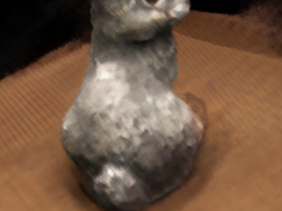
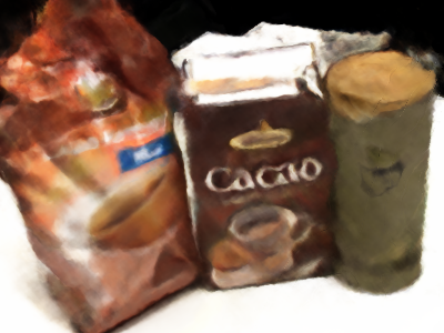
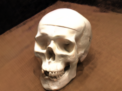
w/ fine-tuning 100k iters

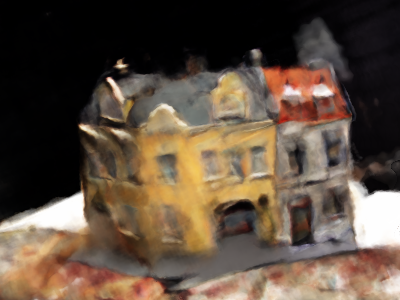
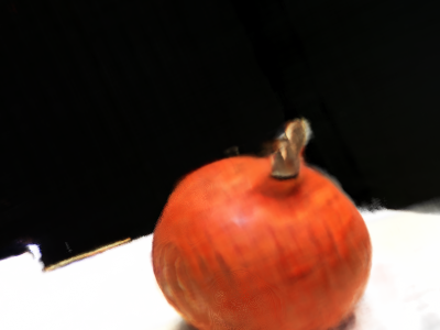
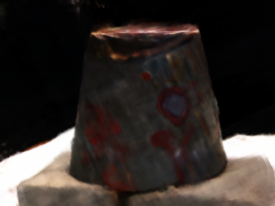
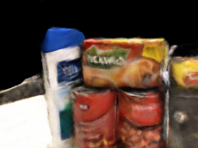
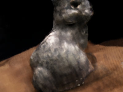
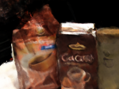
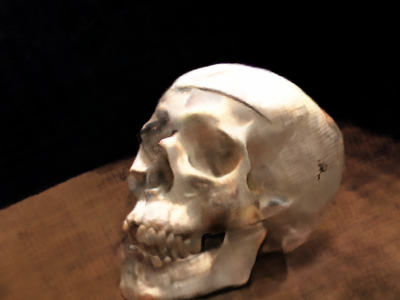
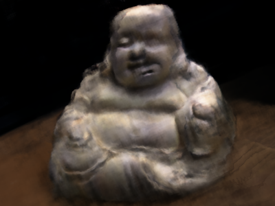
Figure 11: Qualitative results of fine-tuning.

References

- [1] Ben Mildenhall, Pratul P. Srinivasan, Matthew Tancik, Jonathan T. Barron, Ravi Ramamoorthi, and Ren Ng. NeRF: Representing scenes as neural radiance fields for view synthesis. Communications of the ACM, 65(1):99–106, December 2021.
- [2] James T Kajiya and Brian P Von Herzen. Ray tracing volume densities. ACM SIGGRAPH Computer Graphics, 18(3):165–174, July 1984.
- [3] Kai Zhang, Gernot Riegler, Noah Snavely, and Vladlen Koltun. NeRF++: Analyzing and improving neural radiance fields. arXiv:2010.07492, October 2020.
- [4] Thomas Müller, Alex Evans, Christoph Schied, and Alexander Keller. Instant neural graphics primitives with a multiresolution hash encoding. ACM Transactions on Graphics, 41(4):1–15, July 2022.
- [5] Ricardo Martin-Brualla, Noha Radwan, Mehdi S M Sajjadi, Jonathan T Barron, Alexey Dosovitskiy, and Daniel Duckworth. NeRF in the wild: Neural radiance fields for unconstrained photo collections. In Proceedings of the 2021 IEEE/CVF Conference on Computer Vision and Pattern Recognition (CVPR), June 2021.
- [6] Zirui Wang, Shangzhe Wu, Weidi Xie, Min Chen, and Victor Adrian Prisacariu. NeRF: Neural radiance fields without known camera parameters. arXiv preprint arXiv:2102.07064, February 2021.
- [7] Allan Zhou, Moo Jin Kim, Lirui Wang, Pete Florence, and Chelsea Finn. NeRF in the palm of your hand: Corrective augmentation for robotics via novel-view synthesis. arXiv preprint arXiv:2301.08556, 2023.
- [8] Ajay Jain, Matthew Tancik, and Pieter Abbeel. Putting NeRF on a diet: Semantically consistent few-shot view synthesis. In Proceedings of the 18th IEEE/CVF International Conference on Computer Vision (ICCV), pages 5885–5894, October 2021.
- [9] Hiroshi Murase and Shree K Nayar. Visual learning and recognition of 3-D objects from appearance. International Journal of Computer Vision, 14(1):5–24, January 1995.
- [10] Ian Goodfellow, Jean Pouget-Abadie, Mehdi Mirza, Bing Xu, David Warde-Farley, Sherjil Ozair, Aaron Courville, and Yoshua Bengio. Generative adversarial networks. Communications of the ACM, 63(11):139–144, October 2020.
- [11] Diederik P Kingma and Max Welling. Auto-Encoding variational bayes. arXiv:1312.6114v10, December 2013.
- [12] In-Ho Choi and Yong-Guk Kim. Deep manifold embedding active shape model for pose invarient face tracking. In Proceedings of the 2018 IEEE International Conference on Big Data and Smart Computing (ICBDSC), pages 578–581, May 2018.
- [13] G. E. Hinton and R. R. Salakhutdinov. Reducing the dimensionality of data with neural networks. Science, 313(5786):504–507, July 2006.
- [14] Alex Yu, Vickie Ye, Matthew Tancik, and Angjoo Kanazawa. PixelNeRF: Neural radiance fields from one or few images. In Proceedings of the IEEE/CVF Conference on Computer Vision and Pattern Recognition (CVPR), pages 4578–4587, June 2021.
- [15] Anpei Chen, Zexiang Xu, Fuqiang Zhao, Xiaoshuai Zhang, Fanbo Xiang, Jingyi Yu, and Hao Su. MVSNeRF: Fast generalizable radiance field reconstruction from multi-view stereo. In Proceedings of the 18th IEEE/CVF International Conference on Computer Vision (ICCV), pages 14124–14133, October 2021.
- [16] Qianqian Wang, Zhicheng Wang, Kyle Genova, Pratul P Srinivasan, Howard Zhou, Jonathan T Barron, Ricardo Martin-Brualla, Noah Snavely, and Thomas Funkhouser. Ibrnet: Learning multi-view image-based rendering. In Proceedings of the IEEE/CVF Conference on Computer Vision and Pattern Recognition (CVPR), pages 4690–4699, June 2021.
- [17] Kangle Deng, Andrew Liu, Jun-Yan Zhu, and Deva Ramanan. Depth-supervised nerf: Fewer views and faster training for free. In Proceedings of the 2022 IEEE/CVF Conference on Computer Vision and Pattern Recognition (CVPR), pages 12882–12891, 2022.
- [18] Mijeong Kim, Seonguk Seo, and Bohyung Han. InfoNeRF: Ray entropy minimization for few-shot neural volume rendering. In Proceedings of the 2022 IEEE/CVF Conference on Computer Vision and Pattern Recognition (CVPR), pages 12912–12921, June 2022.
- [19] Michael Niemeyer, Jonathan T Barron, Ben Mildenhall, Mehdi SM Sajjadi, Andreas Geiger, and Noha Radwan. RegNeRF: Regularizing neural radiance fields for view synthesis from sparse inputs. In Proceedings of the 2022 IEEE/CVF Conference on Computer Vision and Pattern Recognition (CVPR), pages 5480–5490, June 2022.
- [20] Alexey Dosovitskiy, Lucas Beyer, Alexander Kolesnikov, Dirk Weissenborn, Xiaohua Zhai, Thomas Unterthiner, Mostafa Dehghani, Matthias Minderer, Georg Heigold, Sylvain Gelly, Jakob Uszkoreit, and Neil Houlsby. An image is worth 16x16 words: Transformers for image recognition at scale. Proceedings of the 9th International Conference on Learning Representations (ICLR), 2021.
- [21] Alec Radford, Jong Wook Kim, Chris Hallacy, Aditya Ramesh, Gabriel Goh, Sandhini Agarwal, Girish Sastry, Amanda Askell, Pamela Mishkin, Jack Clark, Gretchen Krueger, and Ilya Sutskever. Learning transferable visual models from natural language supervision. In Proceedings of the 38th International Conference on Machine Learning (ICML), volume 139, pages 8748–8763, February 2021.
- [22] Hiroshi Ninomiya, Yasutomo Kawanishi, Daisuke Deguchi, Ichiro Ide, Hiroshi Murase, Norimasa Kobori, and Yusuke Nakano. Deep manifold embedding for 3D object pose estimation. In Proceedings of the 12th International Joint Conference on Computer Vision, Imaging and Computer Graphics Theory and Applications, February 2017.
- [23] Yasutomo Kawanishi, Daisuke Deguchi, Ichiro Ide, and Hiroshi Murase. -GAN: Object manifold embedding GAN for image generation by disentangling parameters into pose and shape manifolds. Proceedings of the 25th International Conference on Pattern Recognition (ICPR), January 2021.
- [24] Zhiqiang Gong, Weidong Hu, Xiaoyong Du, Ping Zhong, and Panhe Hu. Deep manifold embedding for hyperspectral image classification. IEEE Transactions on Cybernetics, 52(10):10430–10443, April 2022.
- [25] Zelin Zang, Siyuan Li, Di Wu, Jianzhu Guo, Yongjie Xu, and Stan Z Li. Deep manifold embedding of attributed graphs. Neurocomputing, 514:83–93, December 2022.
- [26] Ken Shoemake. Animating rotation with quaternion curves. In Proceedings of the 12th annual conference on Computer graphics and interactive techniques, SIGGRAPH ’85, pages 245–254, July 1985.
- [27] Zhou Wang, A C Bovik, H R Sheikh, and E P Simoncelli. Image quality assessment: from error visibility to structural similarity. IEEE Transactions on Image Processing, 13(4):600–612, April 2004.
- [28] Richard Zhang, Phillip Isola, Alexei A Efros, Eli Shechtman, and Oliver Wang. The unreasonable effectiveness of deep features as a perceptual metric. In Proceedings of the 2018 IEEE Conference on Computer Vision and Pattern Recognition (CVPR), pages 586–595, June 2018.
- [29] Rasmus Jensen, Anders Dahl, George Vogiatzis, Engil Tola, and Henrik Aanæs. Large scale multi-view stereopsis evaluation. In Proceedings of the 2014 IEEE Conference on Computer Vision and Pattern Recognition (CVPR), pages 406–413, June 2014.
- [30] Berk Calli, Arjun Singh, Aaron Walsman, Siddhartha Srinivasa, Pieter Abbeel, and Aaron M Dollar. The YCB object and model set: Towards common benchmarks for manipulation research. In Proceedings of the 2015 International Conference on Advanced Robotics (ICAR), pages 510–517, September 2015.
- [31] Ben Mildenhall, Pratul P Srinivasan, Matthew Tancik, Jonathan T Barron, Ravi Ramamoorthi, and Ren Ng. NeRF: Representing scenes as neural radiance fields for view synthesis. Computer Vision – ECCV 2020, pages 405–421, 2020.