On Q-balls in Anti de Sitter Space

Abstract

We perform a general analysis of thin-wall Q-balls in AdS space. We provide numeric solutions and highly accurate analytic approximations over much of the parameter space. These analytic solutions show that AdS Q-balls exhibit significant differences from the corresponding flat space solitons. This includes having a maximum radius beyond which the Q-balls are unstable to a new type of state where the Q-ball coexists with a gas of massive particles. The phase transition to this novel state is found to be a zero-temperature third-order transition. This, through the AdS/CFT correspondence, has implications for a scalar condensate in the boundary theory.

I Introduction

The AdS/CFT correspondence Aharony:1999ti , which relates a theory in an anti-de-Sitter (AdS) space in $D+1$ dimensions with a conformal field theory in $D$ dimensions, has been the subject of intense study for many years now. Any observable quantity in the gravitational theory (sometimes called the bulk theory) has a corresponding quantity in the boundary theory e.g. the correlation functions of the field theory are in one-to-one correspondence with the boundary-to-boundary propagators in the bulk theory. The original correspondence of Maldacena:1997re has since been generalized to many other theories.

When the field theory is at nonzero temperature, it can exhibit phase transitions. In the bulk theory, these often correspond to a formation or alteration of bound states. For example, when the temperature of the field theory is increased, there is a deconfinement phase transition; this is believed to correspond to the formation of a black hole Witten:1998zw . AdS can also support other solitons such as boson stars, compact objects made of scalar fields with gravitational (and potentially gauge) interactions  Astefanesei:2003qy ; Prikas:2004yw ; Nogueira:2013if ; Brihaye:2013hx ; Buchel:2013uba ; Kichakova:2013sza ; Kumar:2016sxx ; Brihaye:2022oaf . These solitons exhibit yet other types of phenomena; for instance, if one considers charged boson stars, one can find a zero-temperature second order phase transition between two types of boson stars Hu:2012dx .

In this work we consider a different type of soliton in AdS. Q-balls are configurations of complex scalars $\phi$ that are bound together by self-interactions Coleman:1985ki (Q-balls can also carry a $U(1)$ gauge charge, but here we consider Q-balls whose binding energy is dominated by the scalar attraction). They are stable over a large range of parameter space, and are hence an example of a nontopological soliton.

As Q-balls are solitons in a scalar field theory, their profiles are the solutions to a nonlinear differential equation. While this differential equation is difficult to solve exactly, extremely accurate approximation methods have been found in Heeck:2020bau . These methods produce excellent analytic approximations to the charge and energy of both global Heeck:2020bau and gauged Q-balls Heeck:2021zvk , as well as excited Q-balls Almumin:2021gax and Q-shells Heeck:2021bce ; Heeck:2021gam .

Here we extend these methods to study Q-balls in AdS (some previous work on this subject is Hartmann:2012wa ; Hartmann:2013kna ). We here ignore the backreaction and hence the AdS is taken to be a fixed background for the scalar field. We find solutions both numerically, and by an extension of the methods of Heeck:2020bau , and show excellent agreement. These agree in showing that there is generically a maximal radius for Q-balls in AdS, except for a special class of scalar potentials such as those studied in Hartmann:2012wa . Beyond the corresponding maximal charge, we find an unexpected phase of the theory, where the Q-ball coexists with a gas of noninteracting massive particles (a similar phenomenon has been found for Kerr black holes in AdS Kim:2023sig ).

We also examine the consequences of the Q-ball physics for the dual theory on the boundary. We find an intricate phase diagram with zero-temperature phase transitions that can be either second-order, or surprisingly, even third order. These high order phase transitions are found to be generic for a large class of potentials, as long as they admit Q-ball solutions.

In the next section we review the action for Q-balls in AdS and find the equation for a spherical Q-ball. We then apply approximation techniques to find a relation between the radius of the Q-ball and the parameters of the theory and in the following section, we compare with numerical results to show agreement. The consequences of our analytic understanding of Q-balls are then explored along with the implication for the holographic theory on the boundary. We close with a discussion of our results.

II Q-balls in Anti-de Sitter

We consider a complex scalar field propagating in a fixed Anti-de Sitter background. The AdS geometry is parameterized as

$$ds^{2}=a(r)dt^{2}-b(r)dr^{2}-r^{2}\left(d\theta^{2}+\sin^{2}\theta d\phi^{2}\right)~{},$$ (1)

with

$$a(r)=1+\frac{r^{2}}{\ell^{2}}~{},\ \ b(r)=\frac{1}{1+\frac{r^{2}}{\ell^{2}}}~{},$$ (2)

where $\ell$ is a scale that sets the size of the AdS space.

The action for a scalar field propagating in this geometry is

$$S=\int d^{4}x\sqrt{-g}\left[\left(\nabla_{\mu}\Phi\right)^{\ast}\left(\nabla^{\mu}\Phi\right)-U(\Phi\Phi^{\ast})\right]~{},$$ (3)

The complex scalar field $\Phi$ is subject to a potential $U(\Phi\Phi^{\ast})$ that preserves a global $U(1)$ symmetry and thereby leads to a conserved particle number, denoted by $Q$

$$Q=i\int d^{3}\sqrt{-g}\left(\Phi^{\ast}\partial_{t}\Phi-\Phi\partial_{t}\Phi^{\ast}\right)~{}.$$ (4)

The energy stored in the field

$$E=\int d^{3}x\sqrt{-g}T^{t}_{\phantom{t}t}~{},$$ (5)

is given in terms of the energy-momentum tensor

$$T_{\mu\nu}=\left(\nabla_{\mu}\Phi\right)^{\ast}\left(\nabla_{\nu}\Phi\right)+\left(\nabla_{\nu}\Phi\right)^{\ast}\left(\nabla_{\mu}\Phi\right)-g_{\mu\nu}\left[\left(\nabla_{\mu}\Phi\right)^{\ast}\left(\nabla^{\mu}\Phi\right)-U(\Phi\Phi^{\ast})\right]~{}.$$ (6)

The equation for $\Phi$ is

$$\nabla_{\mu}\nabla^{\mu}\Phi=-\frac{\partial U}{\partial\Phi^{\ast}}=-\Phi\frac{dU}{d(\Phi\Phi^{\ast})}~{},$$ (7)

We look for spherical Q-ball solutions; this implies that we take the scalar field to be of the form

$$\Phi=\frac{\phi_{0}}{\sqrt{2}}f(r)e^{-i\omega t}~{},$$ (8)

where $\phi_{0}/\sqrt{2}$ is the value of the nontrivial minimum of $U(\Phi\Phi^{\ast})/(\Phi\Phi^{\ast})$. To make connection with the typical flat space characterization of Q-balls we also define

$$\omega_{0}^{2}\equiv\left.\frac{U(\Phi\Phi^{\ast})}{\Phi\Phi^{\ast}}\right|_{\Phi=\phi_{0}/\sqrt{2}}~{}.$$ (9)

The dimensionless function $f(r)$ is referred to as the profile of the field configuration. The equation of motion for the field can then be written as an equation to determine this profile

$${d^{2}f\over dr^{2}}+\frac{2}{r}\frac{1+2r^{2}/\ell^{2}}{1+r^{2}/\ell^{2}}{df\over dr}=\frac{f}{1+r^{2}/\ell^{2}}\left(\frac{dU}{d(\Phi\Phi^{\ast})}-\frac{\omega^{2}}{1+r^{2}/\ell^{2}}\right)~{}.$$ (10)

Note that as $\ell\to\infty$ this becomes the usual flat space equation for $f$ Coleman:1985ki .

In general, the equation for $f$ cannot be solved analytically. In this study we focus, following Heeck:2020bau , on a sextic potential

$$U(|\phi|)=m_{\phi}^{2}|\phi|^{2}-\beta|\phi|^{4}+\frac{\xi}{m_{\phi}^{2}}|\phi|^{6}~{}.$$ (11)

While a specific choice, this potential captures the qualities of many potentials that give rise to Q-balls Heeck:2022iky . These potential parameters are mapped to the Q-ball parameters $\phi_{0}$ and $\omega_{0}$ by

$$\phi_{0}=m_{\phi}\sqrt{\frac{\beta}{\xi}}~{},\ \ \ \ \omega_{0}=m_{\phi}\sqrt{1-\frac{\beta^{2}}{4\xi}}~{}.$$ (12)

It is convenient for both numerical analyses and in determining how various quantities depend on the parameters of the theory to define the dimensionless quantities

$$\Phi_{0}=\frac{\phi_{0}}{\sqrt{m_{\phi}^{2}-\omega_{0}^{2}}}~{},\ \ \ \ \Omega_{(0)}=\frac{\omega_{(0)}}{\sqrt{m_{\phi}^{2}-\omega_{0}^{2}}}~{},\ \ \ \ \rho=r\sqrt{m_{\phi}^{2}-\omega_{0}^{2}}~{},\ \ \ \ \lambda=\ell\sqrt{m_{\phi}^{2}-\omega_{0}^{2}}~{}.$$ (13)

The $f$ equation can then be written as

$$f^{\prime\prime}+\frac{2}{\rho}\frac{1+2\rho^{2}/\lambda^{2}}{1+\rho^{2}/\lambda^{2}}f^{\prime} =\frac{f}{1+\rho^{2}/\lambda^{2}}\left[1-\frac{\Omega^{2}}{1+\rho^{2}/\lambda^{2}}+\Omega_{0}^{2}-4f^{2}+3f^{4}\right]~{},$$ (14)

while the charge is

$$Q=4\pi\Phi_{0}^{2}\Omega\int_{0}^{\infty}\mathrm{d}\rho\rho^{2}\frac{f^{2}}{1+\rho^{2}/\lambda^{2}}~{},$$ (15)

and the energy is

$$E= \sqrt{m_{\phi}^{2}-\omega_{0}^{2}}2\pi\Phi_{0}^{2}\int_{0}^{\infty}\mathrm{d}\rho\rho^{2}\left(\frac{\Omega^{2}f^{2}}{1+\rho^{2}/\lambda^{2}}+f^{\prime 2}(1+\rho^{2}\lambda^{2})+f^{2}(1-f^{2})^{2}+\Omega_{0}^{2}f^{2}\right)~{}$$

$$= \omega Q-L~{},$$ (16)

where the Lagrangian is given by

$$L=\sqrt{m_{\phi}^{2}-\omega_{0}^{2}}2\pi\Phi_{0}^{2}\int_{0}^{\infty}\mathrm{d}\rho\rho^{2}\left(\frac{\Omega^{2}f^{2}}{1+\rho^{2}/\lambda^{2}}-f^{\prime 2}(1+\rho^{2}\lambda^{2})-f^{2}(1-f^{2})^{2}-\Omega_{0}^{2}f^{2}\right)~{}.$$ (17)

Using the Lagrangian, one finds that field configurations that satisfy the equations of motion also satisfy

$$\frac{dL}{d\omega}=Q~{},$$ (18)

as in flat space. A straightforward calculation produces

$$\frac{dE}{d\omega}=Q+\omega\frac{dQ}{d\omega}-\frac{dL}{d\omega}=\omega\frac{dQ}{d\omega}~{},$$ (19)

implying that

$$\frac{dE}{dQ}=\omega~{}.$$ (20)

We emphasize that although we have chosen a specific potential, this differential relation relating the energy and charge holds for all potentials. This result also gives $\omega$ a simple interpretation as a chemical potential, describing how the energy changes as the particle number changes.

III Thin-Wall Q-balls

Following Coleman Coleman:1985ki , we can treat Eq. (14) above as describing a particle rolling in a potential $V(f,\rho)$ defined as

$$V(f,\rho)=\frac{f^{2}}{2\left(1+\rho^{2}/\lambda^{2}\right)}\left[\frac{\Omega^{2}}{1+\rho^{2}/\lambda^{2}}-\Omega_{0}^{2}-(1-f^{2})^{2}\right]~{},$$ (21)

where the $\rho$ coordinate is treated as an effective time. Since the potential depends on $\rho$, the physics is of a particle rolling in a time dependent potential. In flat space and in AdS the coefficient of the $f^{\prime}$ term decreases with increasing $\rho$, which is interpreted as a friction that decreases with time. In flat space, thin-wall trajectories are those in which the particle starts rolling from rest near a maximum in the potential but does not complete the large field change, rolling down the hill, until the friction term has become somewhat small. This leads to a fast transition, or a thin-wall for the soliton. All of the Q-ball trajectories end at $f=0$ to ensure a field configuration that is localized in space.

An example of thin-wall Q-balls in AdS, where the field stays at the false minimum of $U$ at $f=f_{+}$ for a long time before making a quick transition to the true minimum of $U$ at $f=0$, is shown in Fig. 1. The left panel shows the Q-ball profile found numerically using collocation algorithms implemented by SciPy 2020SciPy-NMeth . On the right panel, we have shown the effective potential $V(f,\rho)$ as a function of $f$ for several values of $\rho$. The field value at specific value of $\rho$ is shown as a dot.

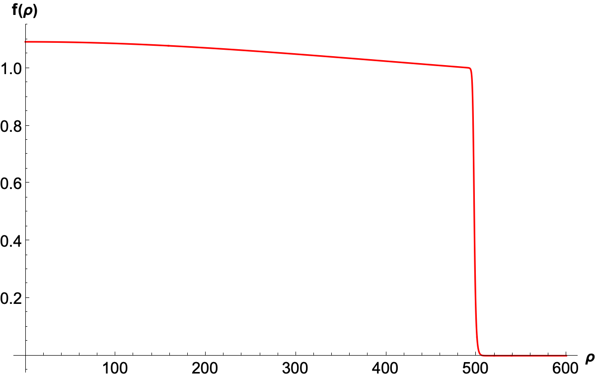
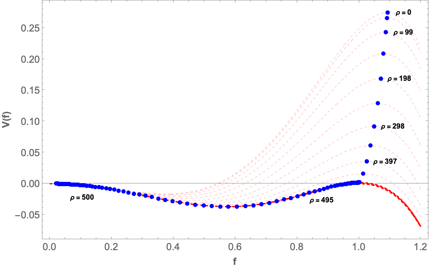
Figure 1: On left: Numerical Q-ball profile for $\lambda=500$ and $\Omega_{0}=1/\sqrt{2}$ , $\Omega=0.99$. On right: effective potential $V(f,\rho)$ for the same parameters and various values of $\rho$, where the blue dots indicate the location of the field value.

The effective potential is found to have extrema at $f=0$ and at

$$f^{2}_{\pm}\equiv\frac{2}{3}\pm\frac{1}{3}\sqrt{1+\frac{3\Omega^{2}}{1+\rho^{2}/\lambda^{2}}-3\Omega_{0}^{2}}~{}.$$ (22)

We note that $f_{+}$ can take real values while $f_{-}$ does not when

$$\Omega^{2}\geq\left(1+\frac{\rho^{2}}{\lambda^{2}}\right)\left(1+\Omega_{0}^{2}\right)~{}.$$ (23)

Within those restrictions we find that $f_{+}$ corresponds to a maximum and $f_{-}$ to a minimum. A more restrictive constraint on Q-ball profiles is that if the “particle” is to roll down a slope that ends at the $f_{+}$ maximum then that maximum must have positive energy, or $V(f,\rho)>0$, for the particle trajectory to overcome the residual friction and end at $f=0$. However, we find that $V(f_{+}(\rho),\rho)=0$ for

$$\rho^{2}=\lambda^{2}\frac{\Omega^{2}-\Omega_{0}^{2}}{\Omega_{0}^{2}}~{}.$$ (24)

Trajectories that have not already rolled to near the $f=0$ maximum by this value of $\rho$ cannot produce a localized soliton configuration. This limits the radius of thin-wall AdS Q-balls to

$$R_{\text{thin-wall}}\lesssim\lambda\frac{\sqrt{\Omega^{2}-\Omega_{0}^{2}}}{\Omega_{0}}~{}.$$ (25)

For flat-space Q-balls the extremum at $f=0$ is always a maximum because $\Omega^{2}-\Omega_{0}^{2}<1$ for Q-ball configurations. In an AdS background, as we see below, this restriction does not apply. Thus, we find that

$$\left.\frac{d^{2}V}{df^{2}}\right|_{f=0}=\frac{\displaystyle\Omega^{2}-\left(1+\rho^{2}/\lambda^{2}\right)\left(1+\Omega_{0}^{2}\right)}{\left(1+\rho^{2}/\lambda^{2}\right)^{2}}~{}.$$ (26)

can lead to a minimum at $f=0$, at least until $\rho$ becomes sufficiently large. Note that this is exactly the same condition for the minimum at $f_{-}$ to not exist. In this case the maximum at $f_{+}$ rolls directly to the minimum at $f=0$. This behavior gives rise to a class of AdS Q-balls with no flat space analogue.

We take the large field transition to occurs at $\rho=R\gg 1$. This implies that for $\rho\ll R$, we should take the solution to be approximately $f=f_{+}(\rho)$. This is not an exact solution to the equations, because the derivatives of $f_{+}(\rho)$ are nonzero, but $f^{\prime}_{+}/f_{+}$ is of order ${1\over\lambda}$, so for $\lambda\gg 1$ the corrections to this solution are small.

On the other hand, when $\rho\sim R$ the field transitions between the two vacua, and the derivatives are not small. To analyze this region, we define an energy-like quantity

$$W= \frac{1}{2}f^{\prime 2}+V(f,\rho)~{},$$ (27)

to analyze the transition region of the Q-ball. For a thin-wall transition we expect this “energy” to be approximately conserved, so $W$ is constant. Note that as $\rho\to\infty$ that $W\to 0$ because the particle comes to rest at $V(0,\infty)=0$. In this approximation we can neglect the contributions to $f^{\prime}$ away from the radius of the soliton, which we define by $f^{\prime\prime}(R)=0$. The equation is then

$$\frac{df}{d\rho}=\sqrt{-2V(f,R)}=\frac{f}{\sqrt{1+R^{2}/\lambda^{2}}}\sqrt{(1-f^{2})^{2}-\frac{\Omega^{2}}{1+R^{2}/\lambda^{2}}+\Omega_{0}^{2}}~{}.$$ (28)

Finally, we expect this equation to be most correct when the particle rolls with the least amount of friction. This would be for cases that come as close as possible to saturating the bound in Eq. (25). In this case the differential equation is

$$\frac{df}{d\rho}=\frac{f}{\sqrt{1+R^{2}/\lambda^{2}}}(1-f^{2})~{},$$ (29)

which leads to the transition profile

$$f_{t}(\rho)=\frac{1}{\sqrt{1+2e^{2(\rho-R)/\sqrt{1+R^{2}/\lambda^{2}}}}}~{}.$$ (30)

To match the interior solution we multiply by $f_{+}(\rho)$. So, our approximate thin-wall profile is

$$f_{T}(\rho)=\frac{f_{+}(\rho)}{\sqrt{1+2e^{2(\rho-R)/\sqrt{1+R^{2}/\lambda^{2}}}}}~{}.$$ (31)

This transition function allows us to capture the leading order effects of friction of the particle trajectories. Using the equations of motion for $f$ we find

$${dW\over d\rho}=-\frac{2}{\rho}\frac{1+2\rho^{2}/\lambda^{2}}{1+\rho^{2}/\lambda^{2}}f^{\prime 2}+\frac{\rho f^{2}}{\lambda^{2}\left(1+\rho^{2}/\lambda^{2}\right)^{2}}\left[\Omega_{0}^{2}-\frac{2\Omega^{2}}{1+\rho^{2}/\lambda^{2}}+\left(1-f^{2}\right)^{2}\right]$$ (32)

By integrating from $\rho=R-z_{0}$ to $\rho=\infty$ we find

$$W_{\infty}-W_{R-z_{0}}= -2\int_{R-z_{0}}^{\infty}\frac{d\rho}{\rho}\frac{1+2\rho^{2}/\lambda^{2}}{1+\rho^{2}/\lambda^{2}}f^{\prime 2}$$

$$+\int_{R-z_{0}}^{\infty}d\rho\frac{\rho f^{2}}{\lambda^{2}\left(1+\rho^{2}/\lambda^{2}\right)^{2}}\left[\Omega_{0}^{2}-\frac{2\Omega^{2}}{1+\rho^{2}/\lambda^{2}}+\left(1-f^{2}\right)^{2}\right]$$ (33)

We find the leading effect from the friction by evaluating these integrals using the transition function defined in Eq. (31), similar to the analysis done in Heeck:2020bau . Equation (33) then yields the relation

$$\Omega_{0}^{2}\left(1+{R^{2}\over\lambda^{2}}\right)-\Omega^{2}=-\frac{1}{R}\left[1+{R^{2}\over\lambda^{2}}\right]^{3/2}+{R\over\lambda^{2}}{{2\Omega^{2}\ln 2}\over\sqrt{1+R^{2}/\lambda^{2}}}~{}.$$ (34)

IV Numerics

We begin by verifying that our analytic understanding of Q-balls in AdS agrees with numerical solutions. Solutions to the profile equation (14) were obtained numerically through the use of SciPy 2020SciPy-NMeth . We consider two benchmark points, corresponding to (a) $\lambda=500,\,\Omega_{0}=1/\sqrt{2}$ and (b) $\lambda=100,\,\Omega_{0}=1/10$. For each benchmark point, solutions were generated for various choices of $\Omega$.

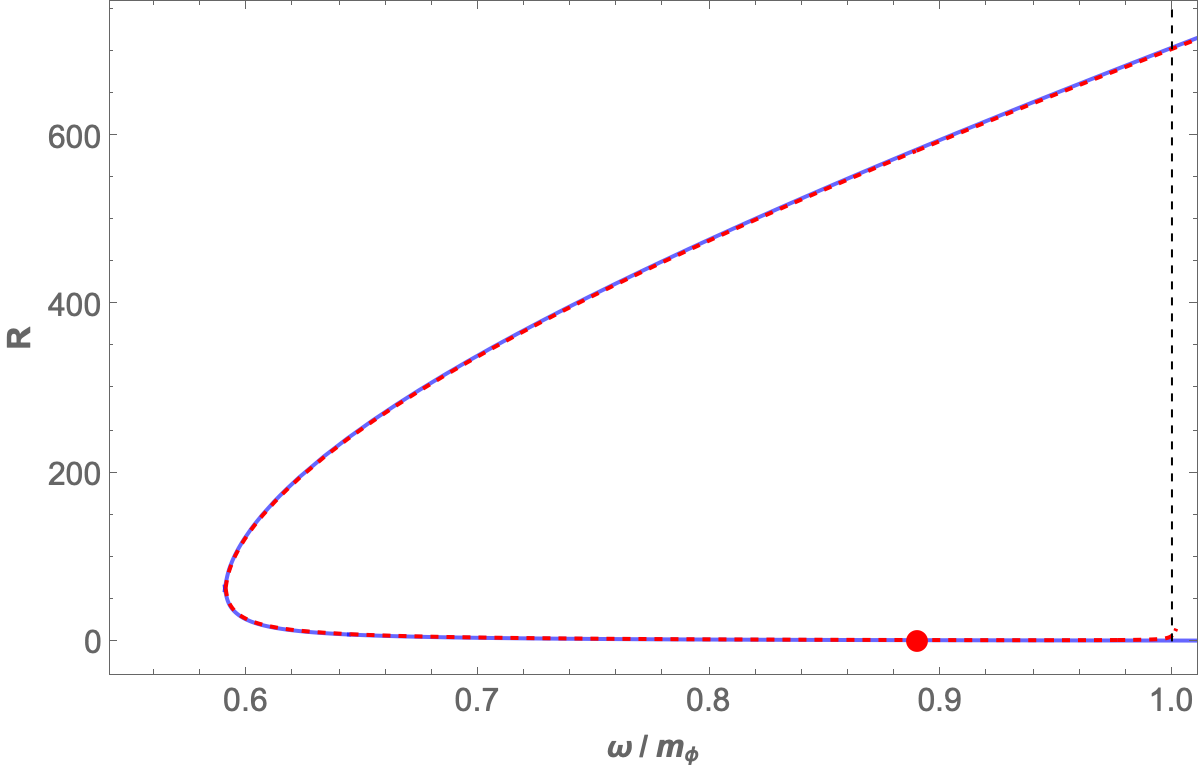
Figure 2: Numerical calculations (red dashed) compared to analytic predictions (blue) for $\lambda=500,\,\Omega_{0}=1/\sqrt{2}$. Left panel: Q-ball radius $R$ as a function of $\omega$. Right panel: Both Q-ball profiles for $\Omega=0.99$.

Figure 2 shows the comparison between the numerical calculations (red dashed) and analytic predictions (blue) for the benchmark point $\lambda=500,\Omega_{0}=1/\sqrt{2}$. The left panel shows the obtained numeric values for the Q-ball radius $R$ as a function of $\omega$ with a comparison to the analytic predictions from Eq. (34). The difference between the numerical and analytical results is negligible. The vertical dashed line is $\omega=m_{\phi}$ or $\Omega=\sqrt{1+\Omega_{0}^{2}}$. In flat space there are no Q-ball solutions beyond this point, but we find both numerical and theoretical evidence for these solitons in AdS space. The red dot indicates the $E=mQ$ instability point which is described below. Soliton solutions to the right of this point on the curve are unstable to dissociation.

The right panel of Fig. 2 compares the numerical and analytic predictions (as predicted by (31)) for the two Q-ball profiles for the same parameters $\lambda=500,\,\Omega_{0}=1/\sqrt{2}$ and $\Omega=0.99$. The two different solutions for $R$ lead to two different profile functions of very different radius. Once again, the difference between the numerical and analytical results is negligible for both profiles.

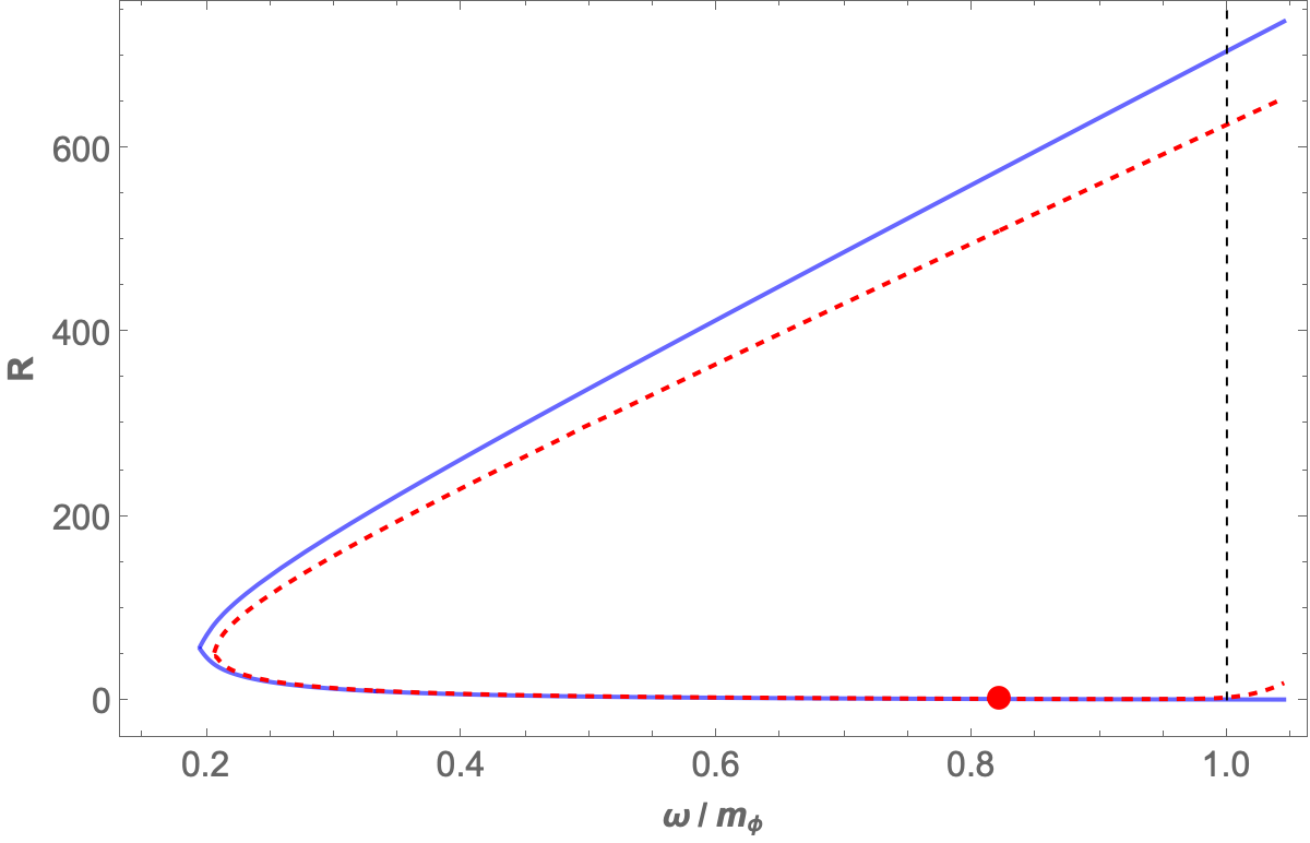
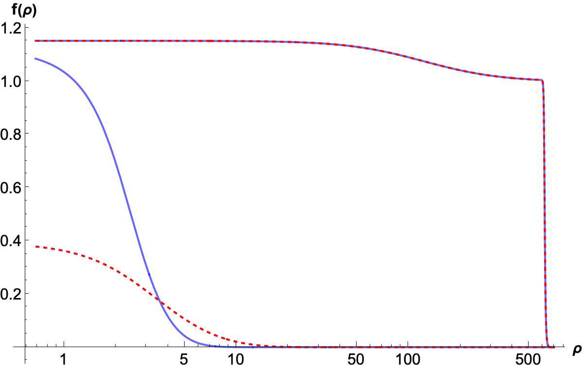
Figure 3: As in Fig. 2, but for the benchmark point $\lambda=100,\,\Omega_{0}=1/10$. Red dashed curves are numerical results, blue curves are the analytic predictions.

Figure 3  is similar to Fig. 2, except that the benchmark point is $\lambda=100,\Omega_{0}=1/10$. In this case, we notice a small (about 10%) difference between the numeric and analytic results regarding the radius of the Q-balls. It would be interesting to study how to modify our prediction to obtain better accuracy for larger AdS curvature. This miscalculation of the radius does, of course, feed into the profile prediction. However, as seen in the right panel of Fig. 3 when we correct for the radius the functional form of the analytic thin-wall profile remains impressively accurate. The profile with smaller radius is not fit well by our analytic profile. This is because our calculation assumed the particle begins rolling from the maximum of the potential, but for these profiles the particle begins rolling some way downhill of the maximum.

As can be seen, there is overall an excellent match between the analytical predictions from the previous section and the numerical results near the thin-wall limit.

We emphasize that from the figures, unlike in flat space Coleman:1985ki , there are AdS Q-balls for $\omega>m_{\phi}$. We have shown this for two benchmarks, but it seems to apply quite generally. As discussed in the previous section, in the full profile equation (14), the term proportional to $\Omega$ is itself suppressed at large $\rho$, and so we can have solutions that are localized, even if $\omega>m_{\phi}$.

V Instabilities

In this section we discuss two different instabilities related to global Q-balls. The first is familiar from flat-space solitons, but the second is new to the AdS case.

(a) There exist solutions to the field equation with $E/Q>m_{\phi}$ and $\frac{dE}{dQ}<m_{\phi}$, where $E$ is the energy, and $Q$ is the global charge. At this point the Q-ball is unstable to decay to $Q$ individual, independent particles of mass $m_{\phi}$. The emission of just a few particles does not stabilize the soliton because $\frac{dE}{dQ}=\omega<m_{\phi}$, so shedding individual charged particles makes $E/Q$ even larger. The lowest energy state with this charge is expected to be a gas of free particles without any soliton.

(b) In AdS, though not in flat space, we can have ${dE\over dQ}>m_{\phi}$. In this case, removing a particle from the Q-ball decreases the energy of the system, as the energy required to remove the particle is more than compensated by the binding energy. Such a Q-ball will therefore radiate particles until it reaches a state with ${dE\over dQ}=m_{\phi}$, with an additional gas of free particles of mass $m_{\phi}$. From the relation ${dE\over dQ}=\omega$, we find that if for a global charge $Q$ the Q-ball solution has $\omega<m_{\phi}$ it remains a pure Q-ball solution. Conversely, if for a fixed charge $Q$ the soliton solution has $\omega>m_{\phi}$ it sheds particles leading to a field configuration with a Q-ball plus additional unbound particles.

These instability points are marked for the benchmark points in Figs. 2 and 3. The red dot indicates the point at which $E=m_{\phi}Q$; to the right of this point, the lower branch becomes unstable to a state completely composed of free particles. We have also shown the line $\omega=m_{\phi}$. To the right of this line we have ${dE\over dQ}>m_{\phi}$ and the upper branch becomes unstable to a soliton of smaller charge surrounded by a gas of free particles.

The implication is that in AdS generically, there is, first, a minimum charge $Q_{\text{min}}$ for Q-balls below which $E=m_{\phi}Q$ and the soliton dissolves into particles. Second, a maximum charge $Q_{\text{max}}$ for Q-balls where $\omega=m_{\phi}$, and beyond which a gas of particles forms around the Q-ball. Third, the two branches of solutions as function of $\omega$ shows that there is a charge $Q$ where the frequency $\omega$ is minimized to some value $\omega_{min}$.

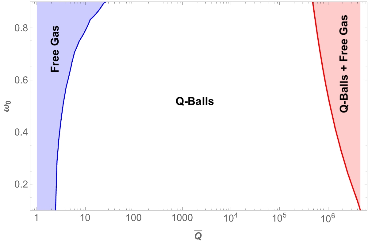
Figure 4: Phase diagram of the theory as a function of $\omega_{0}$ and the total charge $\bar{Q}\equiv Q/4\pi\phi_{0}^{2}$ for $\lambda=100$. The phase on the right (red) appears for Q-balls in the AdS background, but not in flat space.

In Fig. 4 we illustrate the phase diagram of AdS Q-balls as a function of the total charge $Q$ and $\omega_{0}$ for the benchmark value of $\lambda=100$. The phase of a free gas of unbound particles is largely the same as for flat space Q-balls. However, the phase on the right of the diagram cannot occur in flat space.

VI Comments on large Radius AdS Q-balls

It is interesting to note that in AdS space, the thin-wall Q-balls must have a maximal radius. This is easily seen by using the language of a particle rolling in a potential. In the thin-wall approximation, the field stays at the second maximum till it transitions. However, for extremely large $R$, the energy of the second maximum drops below the energy at $f=0$, and the transition can no longer occur. There is therefore a maximum possible radius.

There are two possible avenues to having stable AdS Q-balls with large radii. First, one could consider non-thin-wall solutions where the Q-ball profile rolls slowly between the two maxima. These solutions cannot be treated analytically using our methods, and so the formula (34) does not apply. However, the general argument of the previous paragraph still applies; as $\rho$ increases, the entire potential drops, and eventually the field does not have the energy to return to the final field value at $f=0$.

The other possibility is to consider an entirely different class of potential. The effective potential for the particle is of the form

$$V(f,\rho)={\Omega^{2}f^{2}\over\left(1+{\rho^{2}\over\lambda^{2}}\right)^{2}}-\frac{U(f)}{1+{\rho^{2}\over\lambda^{2}}}~{}.$$ (35)

For large $\rho$, the first term is additionally suppressed, and in our case, we recover similar dynamics to the original sextic potential, where the second maximum is below the maximum at $f=0$. However, we can consider a potential where the first term is always dominant at large $f$; this can happen if $U(f)$ grows slower than $f^{2}$ at large $f$. An example is the exponential potential considered in Hartmann:2012wa , where the potential goes to a constant at large $f$. In this model, the authors of Hartmann:2012wa indeed found Q-balls of arbitrarily large radius and charge. We therefore find that the existence of large Q-balls in AdS is possible, but requires a specific form of potential. We leave this issue for future consideration.

VII Implications in the dual theory

From the AdS/CFT correspondence, we expect our results to have an interpretation in a dual three-dimensional field theory. While the precise nature of this field theory is not determined, we note that the scalar field in the AdS bulk must map to a scalar field operator in the dual boundary theory. This operator is typically a composite of the fundamental fields of the theory. We leave the nature of the fundamental theory unspecified, but assume that it has a low energy limit or sector which is dominated by the interactions of this scalar operator. The bulk potential determines certain properties of this operator, and in particular, the dimension of this operator is Aharony:1999ti

$$\Delta={d\over 2}+\sqrt{{d^{2}\over 4}+\ell^{2}m_{\phi}^{2}}~{},$$ (36)

where $d$ is the dimension of the space and $\ell$ is the AdS radius.

The charge of the $U(1)$ scalar field in AdS maps to a $U(1)$ charge on the boundary. More precisely, by weakly gauging the $U(1)$ global symmetry of bulk theory (so that the gauge field does not affect the structure of the Q-ball) this symmetry would be dual to a global $U(1)$ symmetry on the boundary. By construction, the scalar field operator on the boundary carries a charge under this global $U(1)$, and states created by the action of this operator also carry this global charge.

We can understand the dynamics of this sector, and in particular the structure of the ground state of the theory as a function of the charge $Q$, using the bulk Q-ball solution.

Small charge: From the bulk description, we see that for very small charges, the solution is a gas of free particles. The energy increases proportionally to $Q$ as $E=m_{\phi}Q$ (here $m_{\phi}$ is related to the operator dimension by 36).

Intermediate charge: As we increase the charge, there is a critical value (corresponding to $Q_{\text{min}}$) at which the ground state becomes a condensate carrying charge $Q$. The Q-ball is localized in the interior of the AdS space, and has a nontrivial dependence on the $r$ coordinate. This indicates that the three dimensional field theory condensate has a nontrivial dependence on scale.

At the transition point, the condensate has an energy $E=m_{\phi}Q$. The transition therefore does not lead to a discontinuous jump in the energy. However, the condensate has an energy dependence of the form ${dE\over dQ}=\omega$, in contrast to the free gas which has the relation ${dE\over dQ}=m_{\phi}$. Since the transition occurs at a value $\omega$ which is not equal to $m_{\phi}$ (as seen in Figs. 2 and 3), we see that there is a discontinuity in ${dE\over dQ}$. This is therefore a second order phase transition. As the charge increases further, the condensate becomes increasingly bound till the binding energy per particle reaches a maximum value of $m_{\phi}-\omega_{\text{min}}$.

Large charge: As we continue increasing the charge, the binding energy begins to decrease, and vanishes at $Q_{\text{max}}$. Beyond this point, additional charge is not absorbed into the condensate. However, the condensate does not evaporate; instead the condensate is surrounded by a gas of free particles. More precisely, the condensate carries a charge $Q_{\text{max}}$, and the remaining charge $Q-Q_{\text{max}}$ is in free particles.

As mentioned above, the condensate has an energy dependence of the form ${dE\over dQ}=\omega$. Since the transition occurs exactly at $\omega=m_{\phi}$, the energy dependence is ${dE\over dQ}=m_{\phi}$. This is equal to the change in energy when we add a free particle. This implies that ${dE\over dQ}$ is continuous. However, for the gas around the Q-ball, ${d^{2}E\over dQ^{2}}=0$, while for the Q-ball ${d^{2}E\over dQ^{2}}={d\omega\over dQ}$. Hence ${d^{2}E\over dQ^{2}}$ is discontinuous, which implies that this is a third-order phase transition.

VIII Discussion and Conclusion

In this article we have studied Q-balls in a fixed AdS background, with particular focus on thin-wall Q-balls. The scalar field is subject to a sextic potential (which would allow Q-balls even in the absence of the AdS background), but the general features are expected to apply most, if not all, potentials that support thin-wall solitons. We have shown that the AdS background significantly modifies the physics of these Q-balls, even if gravity is not dynamical. In particular, Q-balls have a maximal radius in AdS, unless the potential is of a very special type.

We have also found new phases of the scalar field that composes the Q-balls which do not exist in flat space. Specifically, for large charges, the lowest energy field configuration is a Q-ball surrounded by a gas of massive particles, while in flat space, the ground state for larger charge is just a Q-ball with larger mass and radius.

The transitions between the states are also of a novel type. At low charges, as the charge is increased, there is a zero-temperature second order phase transition to a Q-ball state. Curiously, at high charges, there is a third-order phase transition to the mixed Q-ball scalar gas state mentioned above. These results imply that the dual boundary theory must also have similar transitions.

In this work case, we are consider Q-balls in a AdS scalar field theory, where we have ignored backreaction on the geometry. This implies that the gravitational interactions of order ${1\over M_{pl}}$ have been dropped, while keeping the curvature scale of the AdS constant. This would correspond in the original AdS/CFT correspondence to taking the $N$ of the dual gauge group to infinity while keeping the t’Hooft coupling $g^{2}N$ fixed.

Including dynamical gravity on the AdS side would be an important next step to see if these phase transitions survive the inclusion of gravity. It would also be interesting to connect these solutions to the known boson star solutions. Finally, it would be interesting to extend these solutions to de Sitter space. We leave these and other questions for future work.

References

- (1) O. Aharony, S. S. Gubser, J. M. Maldacena, H. Ooguri, and Y. Oz, “Large N field theories, string theory and gravity,” Phys. Rept. 323 (2000) 183–386, [hep-th/9905111].
- (2) J. M. Maldacena, “The Large N limit of superconformal field theories and supergravity,” Adv. Theor. Math. Phys. 2 (1998) 231–252, [hep-th/9711200].
- (3) E. Witten, “Anti-de Sitter space, thermal phase transition, and confinement in gauge theories,” Adv. Theor. Math. Phys. 2 (1998) 505–532, [hep-th/9803131].
- (4) D. Astefanesei and E. Radu, “Boson stars with negative cosmological constant,” Nucl. Phys. B 665 (2003) 594–622, [gr-qc/0309131].
- (5) A. Prikas, “Q stars in anti-de Sitter space-time,” Gen. Rel. Grav. 36 (2004) 1841–1869, [hep-th/0403019].
- (6) F. Nogueira, “Extremal Surfaces in Asymptotically AdS Charged Boson Stars Backgrounds,” Phys. Rev. D 87 (2013) 106006, [1301.4316].
- (7) Y. Brihaye, B. Hartmann, and S. Tojiev, “Stability of charged solitons and formation of boson stars in 5-dimensional Anti-de Sitter space-time,” Class. Quant. Grav. 30 (2013) 115009, [1301.2452].
- (8) A. Buchel, S. L. Liebling, and L. Lehner, “Boson stars in AdS spacetime,” Phys. Rev. D 87 no. 12, (2013) 123006, [1304.4166].
- (9) O. Kichakova, J. Kunz, and E. Radu, “Spinning gauged boson stars in anti-de Sitter spacetime,” Phys. Lett. B 728 (2014) 328–335, [1310.5434].
- (10) S. Kumar, U. Kulshreshtha, and D. S. Kulshreshtha, “Charged compact boson stars and shells in the presence of a cosmological constant,” Phys. Rev. D 94 no. 12, (2016) 125023, [1709.09449].
- (11) Y. Brihaye, F. Console, and B. Hartmann, “Charged and radially excited boson stars (in Anti-de Sitter),” Phys. Rev. D 106 no. 10, (2022) 104058, [2209.07978].
- (12) S. Hu, J. T. Liu, and L. A. Pando Zayas, “Charged Boson Stars in AdS and a Zero Temperature Phase Transition,” [1209.2378].
- (13) S. R. Coleman, “Q Balls,” Nucl. Phys. B262 (1985) 263. [Erratum: Nucl. Phys. B269, 744 (1986)].
- (14) J. Heeck, A. Rajaraman, R. Riley, and C. B. Verhaaren, “Understanding Q-Balls Beyond the Thin-Wall Limit,” Phys. Rev. D 103 no. 4, (2021) 045008, [2009.08462].
- (15) J. Heeck, A. Rajaraman, R. Riley, and C. B. Verhaaren, “Mapping Gauged Q-Balls,” Phys. Rev. D 103 no. 11, (2021) 116004, [2103.06905].
- (16) Y. Almumin, J. Heeck, A. Rajaraman, and C. B. Verhaaren, “Excited Q-balls,” Eur. Phys. J. C 82 no. 9, (2022) 801, [2112.00657].
- (17) J. Heeck, A. Rajaraman, R. Riley, and C. B. Verhaaren, “Proca Q-balls and Q-shells,” JHEP 10 (2021) 103, [2107.10280].
- (18) J. Heeck, A. Rajaraman, and C. B. Verhaaren, “The Ubiquity of Gauged Q-Shells,” [2105.02893].
- (19) B. Hartmann and J. Riedel, “Glueball condensates as holographic duals of supersymmetric Q-balls and boson stars,” Phys. Rev. D 86 (2012) 104008, [1204.6239].
- (20) B. Hartmann, B. Kleihaus, J. Kunz, and I. Schaffer, “Compact (A)dS Boson Stars and Shells,” Phys. Rev. D 88 no. 12, (2013) 124033, [1310.3632].
- (21) S. Kim, S. Kundu, E. Lee, J. Lee, S. Minwalla, and C. Patel, “’Grey Galaxies’ as an endpoint of the Kerr-AdS superradiant instability,” [2305.08922].
- (22) J. Heeck and M. Sokhashvili, “Q-balls in polynomial potentials,” Phys. Rev. D 107 no. 1, (2023) 016006, [2211.00021].
- (23) P. Virtanen, R. Gommers, T. E. Oliphant, M. Haberland, T. Reddy, D. Cournapeau, E. Burovski, P. Peterson, W. Weckesser, J. Bright, S. J. van der Walt, M. Brett, J. Wilson, K. J. Millman, N. Mayorov, A. R. J. Nelson, E. Jones, R. Kern, E. Larson, C. J. Carey, İ. Polat, Y. Feng, E. W. Moore, J. VanderPlas, D. Laxalde, J. Perktold, R. Cimrman, I. Henriksen, E. A. Quintero, C. R. Harris, A. M. Archibald, A. H. Ribeiro, F. Pedregosa, P. van Mulbregt, and SciPy 1.0 Contributors, “SciPy 1.0: Fundamental Algorithms for Scientific Computing in Python,” Nature Methods 17 (2020) 261–272.