Soliton resolution and asymptotic stability of $N$-loop-soliton solutions for the Ostrovsky-Vakhnenko equation

Abstract

In this paper, we study the soliton resolution and asymptotic stability of $N$-loop soliton solutions to the Cauchy problem for the Ostrovsky-Vakhenko equation

$$u_{txx}-3\kappa u_{x}+3u_{x}u_{xx}+uu_{xxx}=0,$$

$$u(x,0)=u_{0}(x),$$

where $u_{0}$ is assumed in the Schwartz space satisfying $-u_{0xx}+1>0$. It is shown that the solution of the Cauchy problem can be characterized via a Riemann-Hilbert (RH) problem in a new scale $(y,t)$. Using nonlinear steepest descent method to deform the RH problem, we derive the leading order approximation to the solution of OV equation for long times in the solitonic region of space-time. Our results implies that $N$-loop soliton solutions of the OV equation are symptotically stable.

1 Introduction and main results

In this paper, we study soliton resolution and asymptotic stability of N-loop soliton solutions for the Ostrovsky-Vakhenko (OV) equation on the line

$$u_{txx}-3\kappa u_{x}+3u_{x}u_{xx}+uu_{xxx}=0,$$ (1.1)

$$u(x,0)=u_{0}(x),\quad(x,t)\in\mathbb{R}\times\mathbb{R}^{+},$$ (1.2)

where $\kappa>0$ is a parameter and $u\equiv u(x,t)$ is a real valued function. The equation (1.1) arises in the theory of propagation of surface waves in deep water [1]. This equation can be named as the short wave model of the Degasperis-Procesi equation [2]

$$u_{t}-u_{xxt}+3\kappa u_{x}+4uu_{x}=3u_{x}u_{xx}+uu_{xxx}.$$ (1.3)

Indeed under a scaling transformation

$$x\to\epsilon x,\quad t\to t/\epsilon,\quad u\to\epsilon^{2}u,$$

then (1.3) becomes (1.1) as $\epsilon\to 0$.

In recent years, much work has been done to study the various mathematical properties of the OV equation. For example, as an integrable system, the OV equation can be solved by the inverse scattering method [3]. The initial-boundary value problem for the OV equation on the half-line was investigated via the Fokas unified method [4]. A bi-Hamiltonian formulation for the OV equation was established by using its higher order symmetry and a new transformation to the Caudrey-Dodd-Gibbon-Sawada-Kotera equation [5]. The shock solutions and singular soliton solution, such as peakon, cuspon and loop solitons for OV equation were constructed by developing discontinuous Galerkin method [6]. The well-posedness of the Cauchy problem for the OV equation and its relatives (reduced Ostrovsky equation, generalized Ostrovsky equation, etc.) in Sobolev spaces has been widely studies using analysis techniques [7, 8, 9, 10]. It was shown that the Cauchy problem for the OV equation has a unique global solution $u\in C(\mathbb{R}_{+},H^{3}(\mathbb{R}))$ with initial data $u_{0}\in H^{3}(\mathbb{R})$ and $-u_{0xx}(x)+1>0$, which plays an important role in the integrability of OV equation [11].

For $\kappa=0$ and $\kappa=-1/3$, equation (1.1) respectively reduces to the derivative Burgers equation

$$(u_{t}+uu_{xx})_{xx}=0,$$ (1.4)

and the differentiated Vakhnenko equation [12]

$$(u_{t}+uu_{x})_{x}+u=0.$$ (1.5)

The exact soliton solutions for the equation (1.5) were constructed by applying Hirota bilinear method [13, 14, 15]. These solutions are multi-valued functions having the form of a loop (1-soliton) or many loops (multi-soliton). Without loss of generality, in our paper we assume that $\kappa=1$.

Recently it was shown that the OV equation (1.1) has smooth solitary wave solutions and under the transformation [16, 17]

$$y(x,t):=x-\int_{x}^{\infty}((-u_{xx}+1)^{1/3}-1)d\xi.$$

In the original variable $(x,t)$, the soliton solution of OV equation (1.1) to be a multivalued function having a loop shape, and under the change of variable $y\to x$, which is not monotone, that makes the soliton in the variable $(y,t)$ having a bell shape, which is typical for solitons of integrable nonlinear evolution equations as shown in Fig.1.1.

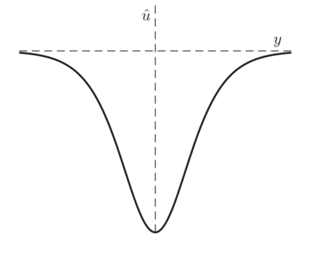
(a) The soliton in the $(y,t)$ variables

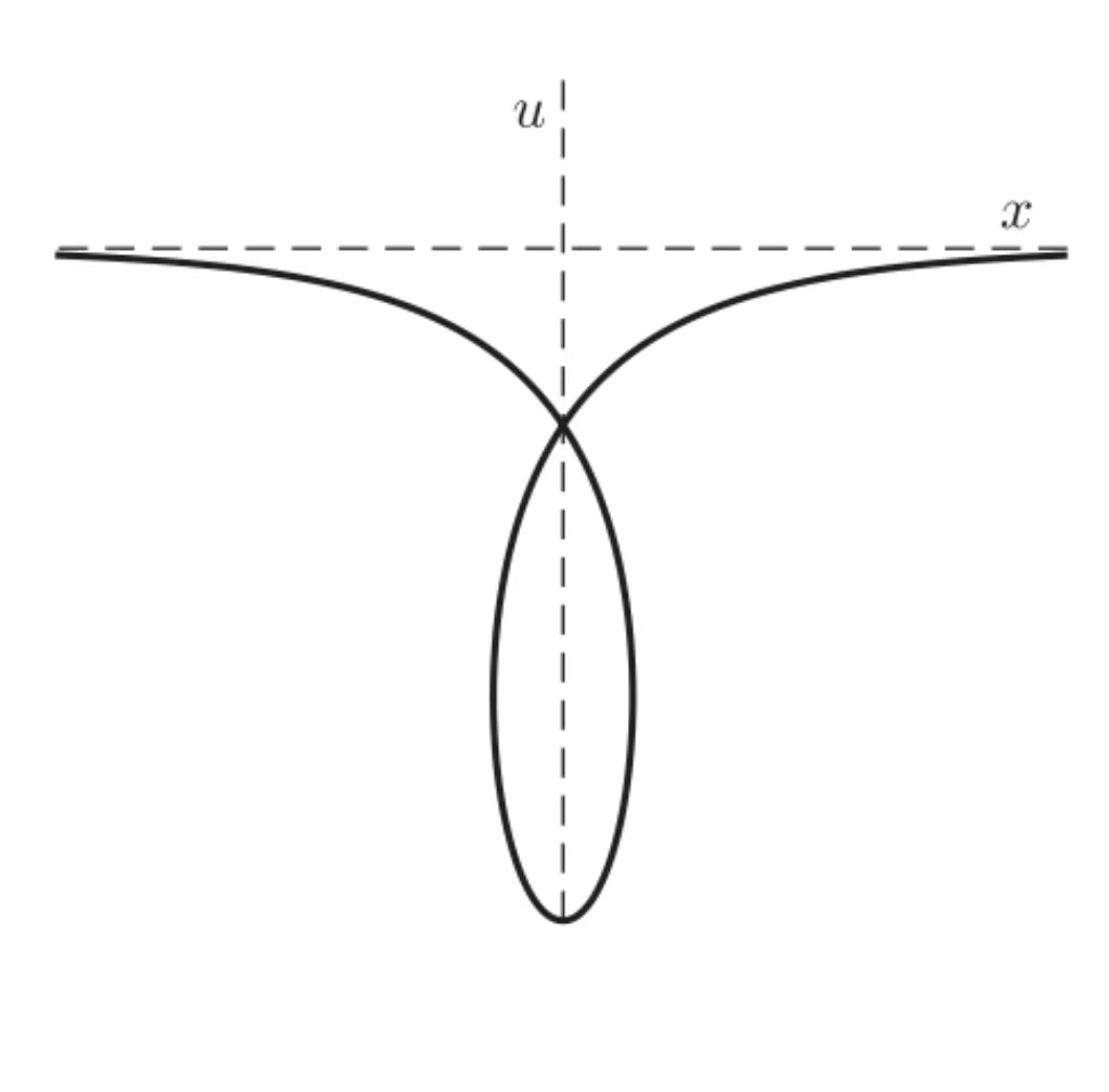
(b) The soliton in the $(x,t)$ variables

Figure 1.1: Expression of soliton in different coordinates

If we assume there are no loop solitons, the pure radiation case is discussed in [16]. It has shown that the OV equation (1.1) has different asymptotic behaviors in different space-time regions. To deduce large-time asymptotics and soliton resolution for (1.1) are established for initial data $u_{0}$ in the following regions:

Figure 1.2: Sectors in the $(x,t)$ half-plane.

• modulated oscillations region: In this region, we can observe loop solitons traveling in the left direction as $t\to\infty$

• soliton region: In this region, we can observe loop solitons traveling in the right direction as $t\to\infty$

From our brief discussion above, one should realize that general solution to the OV equation will consist of loop solitons and radiation term which differently in various space-time regions. In this generic setting, finitely many loop solitons can appear and they interact with the radiation. One might expect that as the consequence of integrability, these nonlinear modes interact elastically during the dynamics but the ways they influence the radiation are remarkably different.

1.1 Soliton resolution

Soliton resolution refers to the property that the solution decompose into the sum of a finite number of separated solitons and a radiative part as $|t|\to\infty$. The limiting soliton parameters are slightly modulated, due to the soliton-soliton and soliton-radiation interactions. We fully describe the dispersive part which contains two components, one coming from the continuous spectrum and another one from the interaction of the discrete and continuous spectrum. This decomposition ia s central feature in nonlinear wave dynamics and has been the object of many theoretical and numerical studies. It has been established in many perturbation contexts, that is when the initial condition is close to a soliton or a multi-soliton. A direct consequence of this result is that $N$-soliton solitons are asymptotically stable.

Our long-time asymptotic will also result in the verification of the soliton resolution conjecture for the OV equation with generic data. This conjecture asserts, roughly speaking, that any reasonable solution eventually resolves into a superposition of a radiation component plus a finite number of “nonlinear bound states” or “solitons”. Soliton resolution along a sequence of times for the focusing energy critical wave equation was studied [18]. By using $\bar{\partial}$-analysis and nonlinear steepest descent method, soliton resolution for the derivative NLS equation was investigated in [19]. In [20], soliton resolution for the focusing modified KdV equation is established. Soliton resolution and large time behavior of solutions to the Cauchy problem for the Novikov equation with a nonzero background was studied in [21]. Our main result is the following detailed soliton resolution for the solution to the OV equation.

Theorem 1.1.

Let $u$ be the solution of the OV equation (1.1), then $u$ can be written as the loop solutions and the radiation as follows

$$u(x,t)=\sum_{j=1}^{6N}u^{(lo)}(x,t)+R(x,t),$$ (1.6)

where the loop soliton $u^{(lo)}(x,t)$ and radiation part $R(x,t)$ are given by

• For the loop solitons part: We have the following asymptotics:

  $$u^{(lo)}(x,t) =\sum_{j=1}^{N^{\prime}}\frac{\hat{e}}{\rho_{j}^{2}}\frac{(\cos(\phi_{j}+\frac{\pi}{3})-\hat{e}+\cos(\phi_{j}+\frac{\pi}{3})\hat{e}^{2})}{(1-4\cos(\phi_{j}+\frac{\pi}{3})\hat{e}+\hat{e}^{2})^{2}}$$

  $$+\sum_{j=1}^{N^{\prime}}\frac{4}{\hat{e}}\frac{(j-1)\cos^{2}(\phi_{j}+\frac{\pi}{3})+\cos(\phi_{j}-\frac{\pi}{3})+\hat{e}}{(\cos(\phi_{j}+\frac{\pi}{3})\hat{e}^{2}+\hat{e})^{2}},$$

  where $\rho,\phi$ is determined by constant $c_{j}$ of residue condition in RH problem 2.1 and

  $$x(y,t)=y+\frac{2\sqrt{3}}{\rho_{j}}\frac{-2\cos(\phi_{j}+\frac{\pi}{3})\hat{e}+\hat{e}^{2}}{1-4\cos(\phi_{j}+\frac{\pi}{3})\hat{e}+\hat{e}^{2}}.$$

  We give the parameter representation for one loop soliton

  $$u^{(lo)}(x,t)=\frac{12}{\rho^{2}}\frac{\hat{e}(\cos(\phi+\frac{\pi}{3})-\hat{e}+\cos(\phi+\frac{\pi}{3})\hat{e}^{2})}{(1-4\cos(\phi+\frac{\pi}{3})\hat{e}+\hat{e}^{2})^{2}},$$ (1.7)

  where

  $$\hat{e}(y,t)=\frac{C}{2\sqrt{3}\rho}e^{-\sqrt{3}\rho(y+\frac{t}{\rho^{2}}-\frac{1}{\sqrt{3}\rho}\log\frac{C}{2\sqrt{3}\rho})},$$

  and $z=\rho e^{i\theta}$ is spectrum parameter and $\phi$ and $C>0$ is constant. The loop solitons have velocity $v=-\frac{1}{\rho^{2}}$, which means loop solitons can travel in both directions.

• For the radiation part: We have the following asymptotics:

  1. In the soliton region,

     $$|R(x,t)|\lesssim t^{-n},\quad n>1.$$ (1.8)

  2. In the modulated oscillations region,

     $$R(x,t)=u_{s}(x,t)+\mathcal{O}(t^{-\frac{\sqrt{3}}{3}-\frac{1}{2}}),$$ (1.9)

where

$$u_{s}(x,t)=\frac{k_{1}}{\sqrt{t}}\cos(\frac{2\sqrt{3}}{\varkappa}t+\nu\log t+k_{2})-\frac{\delta(\omega^{2}z)-\delta(\omega z)}{2z\delta(\omega z)\varkappa^{2}ct^{3/2}}+\mathcal{O}(t^{-\frac{\sqrt{3}}{3}-\frac{1}{2}}),$$

and

$$k_{1}=-2^{3/2}3^{1/4}\sqrt{\frac{\nu}{\varkappa}}\sin\Big{(}\frac{\arg r(\varkappa)-\arg r(-\varkappa)}{2}-\frac{2\pi}{3}\Big{)},$$

$$k_{2}=\nu\log\frac{8\sqrt{3}}{\varkappa}+\frac{\arg r(\varkappa)+\arg r(-\varkappa)}{2}+\arg\Gamma(-i\nu)+\frac{\pi}{4}$$

$$\qquad+\frac{3\varkappa}{\pi}\int_{\varkappa}^{\infty}\frac{\log(1-|r(s)|^{2})}{s^{2}}ds+\frac{1}{\pi}(\int_{-\infty}^{-\varkappa}+\int_{\varkappa}^{\infty})\log|\varkappa-s|d\log(1-|r(s)|^{2})$$

$$\qquad+\frac{1}{2\pi}(\int_{-\infty}^{-\varkappa}+\int_{\varkappa}^{\infty})\frac{\log(1-|r(s)|^{2})(2s+\varkappa)}{s^{2}+s\varkappa+\varkappa^{2}}$$

where $\Gamma$ is the Euler Gamma function and $\nu$ is define in (3.3).

1.2 Asymptotic stability

The full asymptotic stability of multi-loop soliton of the OV equation (1.1) which the by-products of our solitons resolution from the Theorem 1.1.

Theorem 1.2.

Given the loop solitons $u^{(lo)}(x,t,z_{0})$ with the discrete scattering data $(z_{0},c_{0})$ such that $z=\rho e^{i\theta}$, $\rho,\theta>0$ with velocity $v=-\frac{1}{\rho^{2}}<0$. Suppose $\|R(0)\|_{L^{\infty}(\mathbb{R})}<\epsilon$ for $0\leq\epsilon\ll$ small enough, consider the solution $u$ to the OV equation (1.1) with the initial data

$$u_{0}=u^{(lo)}(x,0,z_{0},c_{0})+R(0)$$ (1.10)

Then there exist $z_{1}=\rho_{1}e^{i\theta_{1}}$ and the norming constant $c_{1}$ such that

$$|z_{1}-z_{0}|+|c_{1}-c_{0}|\lesssim\epsilon.$$ (1.11)

Then, we obtain that

$$u=u^{(lo)}(x,t)+R(x,t),$$ (1.12)

where the loop solitons $u^{(lo)}(x,t)$ is given by the scattering data $\{r(z),\{z_{1},c_{1}\}\}$ and the radiation term $R(x,t)$ has the following asymptotics:

1. In the soliton region,

   $$|R(x,t)|\lesssim t^{-n},\quad n>1.$$ (1.13)

2. In the modulated oscillations region,

   $$R(x,t)=u_{s}(x,t)+\mathcal{O}(t^{-\frac{\sqrt{3}}{3}-\frac{1}{2}}),$$

where

$$u_{s}(x,t)=\frac{k_{1}}{\sqrt{t}}\cos(\frac{2\sqrt{3}}{\varkappa}t+\nu\log t+k_{2})-\frac{\delta(\omega^{2}z)-\delta(\omega z)}{2z\delta(\omega z)\varkappa^{2}ct^{3/2}}+\mathcal{O}(t^{-\frac{\sqrt{3}}{3}-\frac{1}{2}}),$$

and

$$k_{1}=-2^{3/2}3^{1/4}\sqrt{\frac{\nu}{\varkappa}}\sin\Big{(}\frac{\arg r(\varkappa)-\arg r(-\varkappa)}{2}-\frac{2\pi}{3}\Big{)},$$

$$k_{2}=\nu\log\frac{8\sqrt{3}}{\varkappa}+\frac{\arg r(\varkappa)+\arg r(-\varkappa)}{2}+\arg\Gamma(-i\nu)+\frac{\pi}{4}$$

$$\qquad+\frac{3\varkappa}{\pi}\int_{\varkappa}^{\infty}\frac{\log(1-|r(s)|^{2})}{s^{2}}ds+\frac{1}{\pi}(\int_{-\infty}^{-\varkappa}+\int_{\varkappa}^{\infty})\log|\varkappa-s|d\log(1-|r(s)|^{2})$$

$$\qquad+\frac{1}{2\pi}(\int_{-\infty}^{-\varkappa}+\int_{\varkappa}^{\infty})\frac{\log(1-|r(s)|^{2})(2s+\varkappa)}{s^{2}+s\varkappa+\varkappa^{2}}$$

where $\Gamma$ is the Euler Gamma function and $\nu$ is define in (3.3).

1.3 Notations

With regard to complex variables, given a variable $z$ or a function $f(z)$, we denote by $\bar{z}$ and $\bar{f}(z)$ their respective complex conjugates.

The symbol $\bar{\partial}$ denoted the derivative with respect to $\bar{z}$, i.e. if $z=x+iy$, then

$$\bar{\partial}f=\frac{1}{2}(f_{x}+if_{y}).$$

Let $C^{\pm}$ are the Cauchy projections:

$$(C^{\pm}f)(z)=\underset{z\to\Sigma_{\pm}}{\lim}\frac{1}{2\pi i}\int_{\Sigma}\frac{f(s)}{s-z}ds.$$

Here $+(-)$ denotes taking the limit from the positive (negative) side of the oriented contour.

As usual, $A:=B$ is definition of $A$ by means of the expression $B$. For positive quantities $a$ and $b$, we write $a\lesssim b$ for $a\leq Cb$ where $C$ is some prescribed constant. Throughout, we use $u_{t}:=\frac{\partial}{\partial_{t}}u$, $u_{x}:=\frac{\partial}{\partial_{x}}u$.

1.4 Outline of this paper

The paper is organized as follows. In Section 2, we report the results on the analyticity, sysmmetries and asymptotics for the Jost functions and scattering data via the inverse scattering transform for the spectral problem (2.1). Then we set up the original RH problem associated with the Cauchy problem (1.1)-(1.2) based on scattering data. In Section 3, we analyze long time asymptotic behavior in region $x/t<\epsilon$ via the $\bar{\partial}$ analysis. We construct a global model solution which captures the leading order asymptotic behavior of the solution, then removing this component of the solution results in a small-norm $\bar{\partial}$ problem. In section 4 we analyze long time asymptotic behavior in region $x/t>\epsilon$ via the steepest descent method.

2 Direct and inverse scattering transforms

2.1 Lax pair

The equation (1.1) is integrable and admits Lax pair [22]

$$\psi_{xxx}=\lambda(-u_{xx}+\kappa)\psi,$$ (2.1a)

$$\psi_{t}=\frac{1}{\lambda}\psi_{xx}-u\psi_{x}+u_{x}\psi,$$ (2.1b)

where $\psi\equiv\psi(t,x;\lambda)$, let $\Phi\equiv\Phi(x,t,z)$ be the matrix-valued function defined by $\Phi=\begin{pmatrix}\psi,\psi_{x},\psi_{xx}\end{pmatrix}^{T}$, then the Lax pair (2.1) can be written in the matrix form

$$\Phi_{x}=\begin{pmatrix}0&1&0\\ 0&0&1\\ z^{3}q^{3}&0&0\end{pmatrix}\Phi,$$ (2.2a)

$$\Phi_{t}=\begin{pmatrix}u_{x}&1&0\\ 0&0&1\\ z^{3}q^{3}&0&0\end{pmatrix}\Phi,$$ (2.2b)

where $q=(-u_{xx}+1)^{1/3}>0$ and $\lambda=z^{3}$. Introduce

$$D(x,t)=\begin{pmatrix}q^{-1}(x,t)&0&0\\ 0&1&1\\ 0&0&q(x,t)\end{pmatrix},$$ (2.3a)

$$P(z)=\begin{pmatrix}1&1&1\\ \lambda_{1}&\lambda_{2}&\lambda_{3}\\ \lambda_{1}^{2}&\lambda_{2}^{2}&\lambda_{3}^{2}\\ \end{pmatrix}\equiv\begin{pmatrix}1&0&0\\ 0&z&0\\ 0&0&z^{2}\\ \end{pmatrix}\begin{pmatrix}1&1&1\\ \omega&\omega^{2}&1\\ \omega^{2}&\omega&1\\ \end{pmatrix},$$ (2.3b)

where $\omega=e^{2\pi i/3}$, $\lambda_{j}(z)=z\omega^{j},j=1,2,3$.

2.2 Jost functions for large $\lambda$

Setting

$$\tilde{\Phi}=P^{-1}D^{-1}\Phi,$$ (2.4)

this leads (2.2) to another Lax pair

$$\tilde{\Phi}_{x}-q\Lambda\tilde{\Phi}=U\tilde{\Phi},$$ (2.5a)

$$\tilde{\Phi}_{t}+(uq\Lambda(z)-\Lambda^{-1}(z))\tilde{\Phi}=V\tilde{\Phi},$$ (2.5b)

where $\tilde{\Phi}\equiv\begin{pmatrix}\tilde{\Phi}_{1}&\tilde{\Phi}_{2}&\tilde{\Phi}_{3}\end{pmatrix}^{T}$ with $\tilde{\Phi}_{j}=\tilde{\Phi}_{j}(x,t,z)$, $j=1,2,3$ and

$$\Lambda=\begin{pmatrix}\lambda_{1}(z)&0&0\\ 0&\lambda_{2}&0\\ 0&0&\lambda_{3}(z)\end{pmatrix}=z\begin{pmatrix}\omega&0&0\\ 0&\omega^{2}&0\\ 0&0&1\end{pmatrix}=z\hat{\Lambda},$$

$$U=\frac{q_{x}}{3q}\begin{pmatrix}0&1-\omega^{2}&1-\omega\\ 1-\omega&0&1-\omega^{2}\\ 1-\omega^{2}&1-\omega&0\end{pmatrix},$$

$$V=-uU+\frac{1}{3z}\Bigg{\{}3\bigg{(}\frac{1}{q}-1\bigg{)}I+\bigg{(}q^{2}-\frac{1}{q}\bigg{)}\begin{pmatrix}1&1&1\\ 1&1&1\\ 1&1&1\end{pmatrix}\Bigg{\}}\begin{pmatrix}\omega^{2}&0&0\\ 0&\omega&0\\ 0&0&1\end{pmatrix},$$

where $\hat{\Lambda}=\mbox{diag}\{\omega,\omega^{2},1\}$ and $I$ is the 3$\times$3 identity matrix. The transformation (2.4) makes $U$ and $V$ are bounded at $z=\infty$ which is appropriate for controlling the behavior of its solutions for large $z$.

For the purpose of considering the eigenfunctions at $z=\infty$, introducing the new variable

$$y(x,t):=x-\int_{x}^{\infty}(q(\xi,t)-1)d\xi,$$ (2.7)

by observing the formula (2.5), one defines $Q$ by

$$Q(x,t,z)=y(x,t)\Lambda(z)+t\Lambda^{-1}(z),$$ (2.8)

and introduce the 3$\times$3 matrix $M\equiv M(x,t,z)$ by

$$M=\tilde{\Phi}e^{-Q}.$$ (2.9)

Then (2.5) reduces to the system

$$M_{x}-[Q_{x},M]=UM,$$ (2.10a)

$$M_{t}-[Q_{t},M]=VM,$$ (2.10b)

whose solutions can be constructed as the Fredholm integral equation whose exponential factors are bounded are determined by the signs of the difference $\mbox{Re}\lambda_{j}(z)-\mbox{Re}\lambda_{l}(z)$, $1\leq j\neq l\leq 3$. Namely, defining

$$\infty_{jl}=\begin{cases}+\infty,\quad\mbox{Re}\lambda_{j}(z)\geq\mbox{Re}\lambda_{l}(z),\\ -\infty,\quad\mbox{Re}\lambda_{j}(z)<\mbox{Re}\lambda_{l}(z),\end{cases}$$ (2.11)

and introduce the set

$$\Sigma=\{z\,|\,\mbox{Re}\,\lambda_{j}(z)=\mbox{Re}\,\lambda_{l}(z)\,\,\mbox{for some}\,\,j\neq l\},$$ (2.12)

that consists of six rays

$$l_{v}=\mathbb{R}_{+}e^{\frac{\pi i}{3}(\nu-1)},\quad\nu=1,\dots,6,$$ (2.13)

dividing the $z$-plane into six sectors,

$$\Omega_{\mu}=\Big{\{}z\,|\,\frac{\pi}{3}(\nu-1)<\mbox{arg}z<\frac{\pi}{3}\nu\Big{\}},\quad\nu=1,\dots,6,$$ (2.14)

and the matrix function $M(x,t;z)$ has to be understood as a collection of scalar Fredholm integral equation

$$M_{jl}(x,t;z)=I_{jl}+\int_{\infty_{jl}}^{x}e^{-\lambda_{j}(z)\int_{x}^{\xi}q(\zeta,t)d\zeta}[(UM)_{jl}(\xi,t;z)]e^{\lambda_{l}(z)\int_{x}^{\xi}q(\zeta,t)d\zeta}.$$ (2.15)

which provide the boundedness as $z\to\infty$. It was shown that the eigenfunction $M(z)$ defined by (2.9) has the following properties [16].

Proposition 2.1.

The equation (2.15) uniquely define 3$\times$3-matrix valued solution $M(z)=M(x,t,z)$ of (2.10) with the following properties:

• $\det M(z)\equiv 1$.

• For spectral parameter $z$, the function $M(z)$ is piecewise meromorphic with respect to $\Sigma$.

• $M(x,t,z)$ satisfies the symmetry relations:

  • (S1) $\Gamma_{1}\overline{M(x,t,\bar{z})}\Gamma_{1}=M(x,t,z)$ with $\Gamma_{1}=\begin{pmatrix}0&1&0\\ 1&0&0\\ 0&0&1\end{pmatrix}$.

  • (S2) $\Gamma_{2}\overline{M(x,t,\bar{z}\omega^{2})}\Gamma_{2}=M(x,t,z)$ with $\Gamma_{2}=\begin{pmatrix}0&0&1\\ 0&1&0\\ 1&0&0\end{pmatrix}$.

  • (S3) $\Gamma_{3}\overline{M(x,t,\bar{z}\omega)}\Gamma_{3}=M(x,t,z)$ with $\Gamma_{3}=\begin{pmatrix}1&0&0\\ 0&0&1\\ 0&1&0\end{pmatrix}=\Gamma_{2}\Gamma_{1}\Gamma_{2}$.
    

  • (S4) $M(x,t,z\omega)=C^{-1}M(x,t,z)C$ with $C=\begin{pmatrix}0&0&1\\ 1&0&0\\ 0&1&0\end{pmatrix}=\Gamma_{2}\Gamma_{1}.$

• According to [23], $M(z)$ is at most a finite number of simple poles lying in $\Omega_{\nu},\nu=1,\dots,6$. The poles may lie only on the lines $\rho e^{\frac{i\pi}{6}+\frac{i\pi m}{3}},\,m=0,\dots,5$ for $\rho>0$ as shown in Fig. 2.1 we denote them as

  $$\mathcal{Z}=\{z_{j},\bar{z}_{j},\omega z_{j},\omega\bar{z}_{j},\omega^{2}z_{j},\omega^{2}\bar{z}_{j}\}_{j=1}^{N}.$$

  which mean for $1\leq j\leq N$, the simplest case involves 6 poles and it does not depend on $(x,t)$.

• $M(x,t,z)$ is bounded as a function of $x$, for all fixed $t$ and $z\in\mathbb{C}$, $z\notin\Sigma\cup\mathcal{Z}$. Moreover, $M(x,t,z)\to I$ as $x\to\infty$.

• $M(x,t,z)\to I$ as $z\to\infty$.

Figure 2.1: Distribution of the discrete spectrum $\mathcal{Z}$.

2.3 Jost functions for small $\lambda$

Setting

$$\hat{\Phi}=P^{-1}\Phi,$$ (2.16)

this leads (2.2) to another Lax pair

$$\hat{\Phi}_{x}-\Lambda(z)\hat{\Phi}=\hat{U}\hat{\Phi},$$ (2.17a)

$$\hat{\Phi}_{t}-\Lambda^{-1}(z))\hat{\Phi}=\hat{V}\hat{\Phi},$$ (2.17b)

where $\hat{\Phi}\equiv\begin{pmatrix}\hat{\Phi}_{1}&\hat{\Phi}_{2}&\hat{\Phi}_{3}\end{pmatrix}^{T}$ with $\hat{\Phi}_{j}=\hat{\Phi}_{j}(x,t,z)$, $j=1,2,3$ and

$$\hat{U}=-\frac{zu_{xx}}{3}\begin{pmatrix}w&0&0\\ 0&w^{2}&0\\ 0&0&1\end{pmatrix}\begin{pmatrix}1&1&1\\ 1&1&1\\ 1&1&1\end{pmatrix},$$

$$\hat{V}=\frac{u_{x}}{3}\begin{pmatrix}0&1-w^{2}&1-w\\ 1-w&0&1-w^{2}\\ 1-w^{2}&1-w&0\end{pmatrix}-zu\begin{pmatrix}w&0&0\\ 0&w^{2}&0\\ 0&0&1\end{pmatrix}\Bigg{\{}I-\frac{u_{xx}}{3}\begin{pmatrix}1&1&1\\ 1&1&1\\ 1&1&1\end{pmatrix}\Bigg{\}}.$$

The transformation (2.7) makes $\hat{U}$ and $\hat{V}$ are bounded at $z=0$ which is appropriate for controlling the behavior of its solutions as $z\to 0$. One defines $\hat{Q}$ by

$$\hat{Q}=e^{x\Lambda+t\Lambda^{-1}},$$ (2.19)

and introduce the 3$\times$3 matrix $\hat{M}\equiv\hat{M}(x,t;z)$ by

$$\hat{M}=\hat{\Phi}e^{-\hat{Q}}.$$ (2.20)

Then (2.5) reduces to the system

$$\hat{M}_{x}-[\hat{Q}_{x},\hat{M}]=\hat{U}\hat{M},$$ (2.21a)

$$\hat{M}_{t}-[\hat{Q}_{t},\hat{M}]=\hat{V}\hat{M},$$ (2.21b)

and the matrix function $\hat{M}(x,t;z)$ has to be understood as a collection of scalar Fredholm integral equation

$$\hat{M}{jl}(x,t;z)=I_{il}-\frac{z}{3}\int_{\infty_{jl}}^{x}e^{\lambda_{j}(z)(x-\xi)}[(u_{xx}\Omega\hat{M})_{jl}(\xi,t;z)]e^{-\lambda_{l}(z)(x-\xi)}d\xi.$$ (2.22)

where $\infty_{jl}$ is defined in (2.11) and $\Omega=\begin{pmatrix}\omega&\omega&\omega\\ \omega^{2}&\omega^{2}&\omega^{2}\\ 1&1&1\end{pmatrix}.$ Similarly to Proposition 2.1, equation (2.22) determines a piecewise meromorphic, 3$\times$3 matrix-valued function $\hat{M}$. Moreover, the particular on $z$ in (2.22) implies a particular form of the first coefficients in the expansion of $\hat{M}$ as $z\to 0$.

Proposition 2.2.

The equation (2.20) uniquely define 3$\times$3-matrix valued solution $M(z)=M(x,t,z)$ of (2.21) with the following properties:

• $\det M(z)\equiv 1$.

• For spectral parameter $z$, the function $\hat{M}(z)$ is piecewise meromorphic with respect to $\Sigma$.

• $\hat{M}(x,t,z)$ satisfies the symmetry relations:

  • (S1)$\Gamma_{1}\overline{\hat{M}(x,t,\bar{z})}\Gamma_{1}=\hat{M}(x,t,z)$ with $\Gamma_{1}=\begin{pmatrix}0&1&0\\ 1&0&0\\ 0&0&1\end{pmatrix}$.

  • (S2)$\Gamma_{2}\overline{\hat{M}(x,t,\bar{z}\omega^{2})}\Gamma_{2}=\hat{M}(x,t,z)$ with $\Gamma_{2}=\begin{pmatrix}0&0&1\\ 0&1&0\\ 1&0&0\end{pmatrix}$.

  • (S3)$\Gamma_{3}\overline{\hat{M}(x,t,\bar{z}\omega)}\Gamma_{3}=\hat{M}(x,t,z)$ with $\Gamma_{3}=\begin{pmatrix}1&0&0\\ 0&0&1\\ 0&1&0\end{pmatrix}=\Gamma_{2}\Gamma_{1}\Gamma_{2}$.
    

  • (S4)$\hat{M}(x,t,z\omega)=C^{-1}\hat{M}(x,t,z)C$ with $C=\begin{pmatrix}0&0&1\\ 1&0&0\\ 0&1&0\end{pmatrix}=\Gamma_{2}\Gamma_{1}.$

• $\hat{M}(x,t,z)$ is bounded as a function of $x$, for all fixed $t$ and $z\in\mathbb{C}$, $z\notin\Sigma\cup\mathcal{Z}$, the set of poles of $\hat{M}(z)$ is $\mathcal{Z}_{0}$. Moreover, $M(x,t,z)\to I$ as $x\to\infty$.

• $M(x,t,z)\to I$ as $z\to 0$. Moreover,

  $$\hat{M}(x,t,z)=I+\hat{M}^{(1)}(x,t)z+M^{(2)}(x,t)z^{2}+\mathcal{O}(z^{3})\quad z\to 0,$$ (2.23)

  where

  $$\hat{M}^{(1)}=-\frac{1}{3}u_{x}\Omega,\quad\hat{M}^{(2)}=-\frac{1}{3}u\tilde{\Omega},$$

  with $\tilde{\Omega}=\hat{\Lambda}\Omega-\Omega\hat{\Lambda}$ and $\hat{\Lambda}=diag\{\omega,\omega^{1},1\}$.

Tracing back the linear system of PDEs (2.1), we notice that $M$ and $\hat{M}$ are related in the following way:

$$M(x,t,z)=G(x,t)\hat{M}(x,t,z)e^{N(x,t)z\hat{\Lambda}},$$ (2.24)

where

$$F(x,t):=x-y(x,t)=\int_{0}^{+\infty}(q(\xi,t)-1)d\xi,$$ (2.25)

and

$$G(x,t):=P^{-1}(z)D^{-1}(x,t)P(z)=\begin{pmatrix}\alpha&\beta&\gamma\\ \gamma&\alpha&\beta\\ \beta&\gamma&\alpha\end{pmatrix},$$

where $P$ and $D$ are as in (2.3) and with

$$\alpha=\bar{\alpha}=\frac{1}{3}\Big{(}q+1+\frac{1}{q}\Big{)},\qquad\beta=\bar{\gamma}=\frac{1}{3}\Big{(}q+\omega+\frac{\omega^{2}}{q}\Big{)}.$$ (2.26)

Remark 2.3.

If $z=0$, then

$$P^{-1}=\frac{1}{3}\begin{pmatrix}1&\omega^{2}&\omega\\ 1&\omega&\omega^{2}\\ 1&1&1\end{pmatrix}\begin{pmatrix}1&0&0\\ 0&z^{-1}&0\\ 0&0&z^{-2}\end{pmatrix},$$

becomes degenerate, the factor $G$ is non-singular. Moreover, it is independent of $z$. From (2.23) and (2.26) we derive the following expansion of $M$ as $z\to 0$:

$$M= G(x,t)\Big{(}I+z\big{\{}-\frac{u_{x}}{3}\Omega+N\hat{\Lambda}\big{\}}$$

$$+z^{2}\big{\{}-\frac{u}{3}\tilde{\Omega}-\frac{u_{x}}{3}N\omega\hat{\Lambda}+\frac{N^{2}}{2}\hat{\Lambda}^{2}\big{\}}+\mathcal{O}(z^{3})\Big{)}.$$ (2.27)

2.4 Scattering data

We consider $z$ on the common boundary of two adjacent domains $\Omega_{\nu}$, the limiting values of $\tilde{\Phi}=Me^{Q}$ being the solutions of the system of differential equation (2.5) must be related by a matrix independent of $(x,t)$. Denote $M_{\pm}(x,t,z)$ as the limiting values of $M(x,t,z^{\prime})$ as $z^{\prime}\to z$ from the positive or negative side of $l_{n}$, then they are related as follows

$$M_{+}(x,t,z)=M_{-}(x,t,z)S(x,t,z),\quad z\in\Sigma,$$ (2.28)

where

$$S(x,t,z)=e^{Q(x,t,z)}S_{0}e^{-Q(x,t,z)},$$ (2.29)

with some matrix $S_{0}$ independent of $(x,t)$ and $\Sigma=l_{1}\cup\dots\cup l_{6}$ as in (2.12).

The matrix $S_{0}$ has a particular structure[26] and only depends on $z$ and is completely determined by the initial data $u_{0}$ for the Cauchy problem (1.1). For example, $z\in l_{1}=\mathbb{R}_{+}$ we have $S_{0}$ have a special matrix structure

$$S_{0}=\begin{pmatrix}1&r_{+}(z)&0\\ -r_{-}(,z)&1-r_{-}r_{+}(z)&0\\ 0&0&1\end{pmatrix},$$ (2.30)

where $r_{\pm}(z)\in L^{\infty}(\mathbb{R}^{\pm})$, and $r_{\pm}(z)=\mathcal{O}(z^{-1})$ as $z\to\pm\infty$. Using similar arguments we get exactly the same structure for $z\in l_{4}=\mathbb{R}_{-}$. Now, by symmetry (S1) from Proposition 2.1, we get that $\Gamma_{1}\overline{S_{0}(z)}\Gamma_{1}=S_{0}^{-1}(z)$ and thus $r_{-}(z)=\overline{r_{+}(z)}$, which we acquire $z\in\mathbb{R}=l_{1}\cup l_{4}$,

$$S_{0}=\begin{pmatrix}1&\bar{r}(z)&0\\ -r(z)&1-|r(z)|^{2}&0\\ 0&0&1\end{pmatrix},$$ (2.31)

Here $r(z):=r_{-}(z)$ lies in Schwartz space [27, 28]. And as $z\to 0$, we have $r(z)=\mathcal{O}(z^{3}),z\in\mathbb{R}$.

In order to finish our following work, we assume our initial data satisfies that $u_{0}\in\mathcal{S}(\mathbb{R})$ to generic scattering data such that $M(z)$ at poles lie only on the lines $\rho e^{\frac{i\pi}{6}+\frac{i\pi m}{3}},\,m=0,\dots,5$ for $\rho>0$.

For initial data $u_{0}\in X_{0}$, the collection $\mathcal{D}=\{r(z),\{z_{k},c_{k}\}_{k=1}^{6N}\}$ is called the scattering data for $u_{0}(x)$ and map $\mathcal{S}:u_{0}\mapsto\mathcal{D}$ is called the forward scattering map. The essential fact of integrability is that if the potential $u_{0}(x)$ evolves according to (1.1) then the evolution of the scattering data $\mathcal{D}$ is trivial

$$\mathcal{D}(t)=\{r(z,t),\{z_{k}(t),c_{k}(t)\}_{k=1}^{6N}\}=\{r(z)e^{t\Lambda^{-1}},\{z_{k},c_{k}(t)e^{t\Lambda^{-1}}\}_{k=1}^{6N}\}.$$

The inverse scattering map $\mathcal{S}^{-1}:\mathcal{D}(t)\mapsto u(x,t)$ seeks to recover the solution of (1.1) from its scattering data.

In what follows, we will assume that $r(z)$ has an analytic extension to a small neighborhood of the real axis. This is , for example, the case if we assume that the solution is exponentially decaying as $|x|\to\infty$. Otherwise one can split $r(z)$ into an analytic part plus a reminder producing a polynomially decaying in $t$ error term, the decay depending on the rate of decay of the initial condition $u_{0}(x)$ as $|x|\to\infty$.

2.5 Set up of a RH problem

The dependence of $S(x,t,z)$ on the parameters $(x,t)$ justifies the use of the variable $y=y(x,t)$ in (2.7). The price to pay for this is that the solution of the initial problem can be given only implicitly, or perimetrically. It will be given in terms of functions in the new scale, whereas the original scale will also be given in terms of functions in the new scale. Indeed, introducing

$$M_{\Diamond}(y,t,z):=M(x(y,t),t,z),$$ (2.32)

(2.7) can be written in terms of the parameters $(y,t)$ as

$$M_{\Diamond+}(y,t,z)=M_{\Diamond-}(y,t,z)S_{\Diamond}(y,t,z),\quad z\in\Sigma,$$ (2.33)

where the jump matrix

$$S_{\Diamond}(y,t,z)=e^{y\Lambda(z)+t\Lambda^{-1}(z)}S_{0}(z)e^{-y\Lambda(z)-t\Lambda^{-1}(z)},$$

is determined in terms of the initial condition $u(x,0)=u_{0}(x)$ and depends explicitly on the parameters $(y,t)$.

RHP 2.1.

Find a analytic function $M_{\Diamond}(y,t;z):\mathbb{C}\setminus(\Sigma\cup\mathcal{Z})\to SL_{3}(\mathbb{C})$ with the following properties:

$\bigstar$(the normalization condition)

$$M_{\Diamond}(y,t,z)=I+\mathcal{O}(z^{-1})\quad z\to\infty.$$

$\bigstar$(the jump condition)

For each $z\in\Sigma=\mathbb{R}\,\cup\,\omega\mathbb{R}\,\cup\,\omega^{2}\mathbb{R}$, the boundary values $M_{\Diamond\pm}$ satisfy the jump relation $M_{\Diamond+}(y,t;z)=M_{\Diamond-}(y,t;z)S_{\Diamond}(y,t;z),\,\,y\in\Sigma$ where the jump matrix

$$S_{\Diamond}(y,t,z)=e^{y\Lambda(z)+t\Lambda^{-1}(z)}S_{0}(z)e^{-y\Lambda(z)-t\Lambda^{-1}(z)},$$ (2.34)

$$S_{\Diamond}(y,t,z) =\begin{pmatrix}1&\bar{r}(z)e^{-2it\theta(\zeta,z)}&0\\ -r(z)e^{2it\theta(\zeta,z)}&1-|r(z)|^{2}&0\\ 0&0&1\end{pmatrix},\qquad\qquad\,\,\,\,\,z\in\mathbb{R},$$

$$=\begin{pmatrix}1-|r(\omega^{2}z)|^{2}&0&-r(\omega^{2}z)e^{2it\theta(\zeta,\omega^{2}z)}\\ 0&1&0\\ \bar{r}(\omega^{2}z)e^{-2it\theta(\zeta,\omega^{2}z)}&0&1\end{pmatrix},\quad z\in\omega\mathbb{R},$$

$$=\begin{pmatrix}1&0&0\\ 0&1&\bar{r}(\omega z)e^{-2it\theta(\zeta,\omega z)}\\ 0&-r(\omega z)e^{2it\theta(\zeta,\omega z)}&1-|r(\omega z)|^{2}\end{pmatrix},\qquad\,\,\,\,z\in\omega^{2}\mathbb{R},$$

$\bigstar$(Singularities)

As $z\to 0$, the limit of $M(z)$ has pole singularities:

$$M_{\Diamond}(y,t,0)=\begin{pmatrix}\alpha&\beta&\gamma\\ \gamma&\alpha&\beta\\ \beta&\gamma&\alpha\end{pmatrix},$$ (2.35)

where $\alpha(y,t)$ and $\beta(y,t)$ have the form

$$\alpha=\frac{1}{3}\big{(}\hat{q}+1+\frac{1}{\hat{q}}\big{)},\quad\beta=\frac{1}{3}\big{(}\hat{q}+\omega+\frac{\omega^{2}}{\hat{q}}\big{)},$$

with some $\hat{q}(y,t)>0$ such that $\hat{q}\to 1$ as $y\to\infty$.

$\bigstar$(the residue condition)

$M_{\Diamond}(y,t,z)$ has simple poles at $\mathcal{Z}$ in $\Omega_{1}$ at which

$$\underset{z=z_{j}}{Res}M_{\Diamond}(y,t,z)=\underset{z\to z_{j}}{lim}M_{\Diamond}(y,t,z)\begin{pmatrix}0&0&0\\ 0&0&0\\ 0&c_{j}e^{2it\theta(\zeta,z_{j})}&0\\ \end{pmatrix},$$

$$\underset{z=\bar{z}_{j}}{Res}M_{\Diamond}(y,t,z)=\underset{z\to\bar{z}_{j}}{lim}M_{\Diamond}(y,t,z)\begin{pmatrix}0&0&0\\ 0&0&0\\ \bar{c}_{j}e^{-2it\theta(\zeta,\bar{z}_{j})}&0&0\\ \\ \end{pmatrix},$$

$$\underset{z=\omega z_{j}}{Res}M_{\Diamond}(y,t,z)=\underset{z\to\omega z_{j}}{lim}M_{\Diamond}(y,t,z)\begin{pmatrix}0&0&c_{j}e^{2it\theta(\zeta,\omega z_{j})}\\ 0&0&0\\ 0&0&0\\ \end{pmatrix},$$

$$\underset{z=\omega\bar{z}_{j}}{Res}M_{\Diamond}(y,t,z)=\underset{z\to\omega\bar{z}_{j}}{lim}M_{\Diamond}(y,t,z)\begin{pmatrix}0&0&0\\ 0&0&\bar{c}_{j}e^{-2it\theta(\zeta,\omega\bar{z}_{j})}\\ \ 0&0&0\\ \end{pmatrix},$$

$$\underset{z=\omega^{2}z_{j}}{Res}M_{\Diamond}(y,t,z)=\underset{z\to\omega^{2}z_{j}}{lim}M_{\Diamond}(y,t,z)\begin{pmatrix}0&0&0\\ c_{j}e^{2it\theta(\zeta,\omega^{2}z_{j})}&0&0\\ 0&0&0\\ \end{pmatrix},$$

$$\underset{z=\omega^{2}\bar{z}_{j}}{Res}M_{\Diamond}(y,t,z)=\underset{z\to\omega^{2}\bar{z}_{j}}{lim}M_{\Diamond}(y,t,z)\begin{pmatrix}0&\bar{c}_{j}e^{-2it\theta(\zeta,\omega^{2}\bar{z}_{j})}&0\\ 0&0&0\\ 0&0&0\\ \end{pmatrix}.$$

Remark 2.4.

The exist and uniqueness of the RH problem 2.1 is depend on the $\alpha$ and $\beta$ as in (2.24), that constitutes an additional condition that must be imposed on the solution of the RH problem 2.1. This is different from that in the case of classical integrable equation, on the other hand, it is typical for the so-called peakon equations, like the CH and DP equation[25, 26].

The solution $u(x,t)$ of OV equation (1.1) can be expressed $z\to 0$ in terms of the solution $M_{\Diamond}(y,t,z)$ of the matrix RH problem 2.1 and the expression is given in a parametric form:

$$u(x,t)=\hat{u}(y(x,t),t),$$ (2.36)

where

$$x(y,t)=y+\underset{z\to 0}{\lim}\Big{(}\frac{\sum_{j=1}^{3}M_{\Diamond j3}(y,t,z)}{\sum_{j=1}^{3}M_{\Diamond j3}(y,t,0)}-1\Big{)}\frac{1}{z},$$

$$\hat{u}(y,t)=\frac{\partial x(y,t)}{\partial t}.$$

2.6 Stationary saddle points and decay domains

In this section we first consider the structure of the jump matrix $S_{\Diamond}(y,t,z)$. By (2.34) its $(j,l)$ entry can be written

$$S_{\Diamond}(y,t,z)_{jl}=e^{y(\lambda_{j}-\lambda_{l})+t(\lambda_{j}^{-1}-\lambda_{l}^{-1})}S_{0}(z)_{jl}.$$

The exponential factor which is trivial for $j=l$ can otherwise be written as $e^{t(\zeta\nu+\frac{3}{\nu})}$, where $\zeta=\frac{y}{t}$ and $\nu=\lambda_{j}(z)-\lambda_{l}(z)=z(\omega^{j}-\omega^{l})$, Since $(\lambda_{j}(z)-\lambda_{l}(z))^{2}=-3\lambda_{j}(z)\lambda_{l}(z)$ for $j\neq l$ the exponential in (2.34) can be written as

$$e^{y(\lambda_{j}-\lambda_{l})+t(\lambda_{j}^{-1}-\lambda_{l}^{-1})}=e^{y\nu+t\frac{3}{\nu}},$$ (2.38)

For $1\leq j,l\leq 3$, we have

$$\theta_{jl}(z) =\Big{[}\zeta(\lambda_{j}-\lambda_{l})+\Big{(}\frac{1}{\lambda_{j}}-\frac{1}{\lambda_{l}}\Big{)}\Big{]}=(\zeta\nu+\frac{3}{\nu}),$$

and $\nu=\lambda_{j}(z)-\lambda_{l}(z)=z(\omega^{j}-\omega^{l})$. In particular, we have

$$\lambda_{1}(z)-\lambda_{2}(z)=z(\omega-\omega^{2})=zi\sqrt{3},$$

$$\lambda_{1}(z)-\lambda_{3}(z)=z(\omega-1)=-z\sqrt{3}e^{-i\pi/6},$$

$$\lambda_{3}(z)-\lambda_{2}(z)=z(1-\omega^{2})=z\sqrt{3}e^{i\pi/6},$$

that is for the $(1,2)$ entry one has $\nu=i\sqrt{3}z$ and thus

$$e^{t\theta_{12}}=e^{it\sqrt{3}(\zeta z-\frac{1}{z})}=e^{-2it\theta(\zeta,z)},$$

where

$$\theta(\zeta,z)=-\frac{\sqrt{3}}{2}\Big{(}\zeta z-\frac{1}{z}\Big{)},$$ (2.39)

and we also obtain that for the $(1,3)$ entry one have $-\theta(\zeta,\omega^{2}z)$ and for $(3,2)$ entry one have $\theta(\zeta,\omega z)$.

And we have

$$\frac{\partial}{\partial z}\theta(\zeta,z)=-\frac{\sqrt{3}}{2}\big{(}\zeta+\frac{1}{z^{2}}\big{)}=0.$$ (2.40)

1. For the range $\frac{y}{t}>\epsilon$, there is no stationary point on $\mathbb{R}$.

2. For the range $\frac{y}{t}<-\epsilon$, there are exist two stationary points $\pm\varkappa$, where $\varkappa\equiv\varkappa(\zeta)=1/\sqrt{|\zeta|}$.

(a) The distribution of stationary phase points for $\zeta>0$

(b) The distribution of stationary phase points for $\zeta=0$

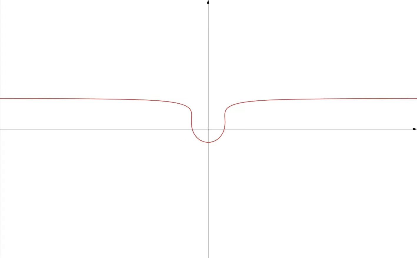
(c) The distribution of stationary phase points for $-2\leq\zeta<0$

(d) The distribution of stationary phase points for $\zeta<-2$

(e) In the case $\zeta>0$, $e^{2it\theta(\zeta,z)}\to 0$ as $|t|\to 0$ in the red region, $e^{-2it\theta(\zeta,z)}\to 0$ as $|t|\to 0$ in the white region

(f) In the case $\zeta<0$, $e^{2it\theta(\zeta,z)}\to 0$ as $|t|\to 0$ in the red region, $e^{-2it\theta(\zeta,z)}\to 0$ as $|t|\to 0$ in the white region

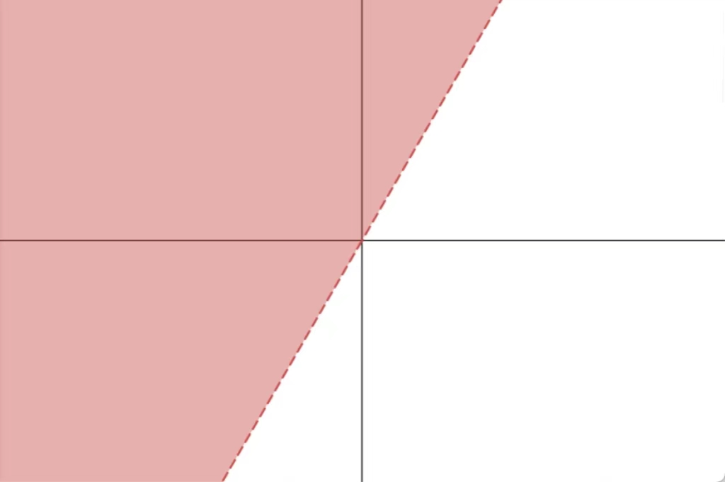
(g) In the case $\zeta>0$, $e^{2it\theta(\zeta,\omega z)}\to 0$ as $|t|\to 0$ in the red region, $e^{-2it\theta(\zeta,\omega z)}\to 0$ as $|t|\to 0$ in the white region

(h) In the case $\zeta<0$, $e^{2it\theta(\zeta,\omega z)}\to 0$ as $|t|\to 0$ in the red region, $e^{-2it\theta(\zeta,\omega z)}\to 0$ as $|t|\to 0$ in the white region

(i) In the case $\zeta>0$, $e^{2it\theta(\zeta,\omega^{2}z)}\to 0$ as $|t|\to 0$ in the red region, $e^{-2it\theta(\zeta,\omega^{2}z)}\to 0$ as $|t|\to 0$ in the white region

(j) In the case $\zeta<0$, $e^{2it\theta(\zeta,\omega^{2}z)}\to 0$ as $|t|\to 0$ in the red region, $e^{-2it\theta(\zeta,\omega^{2}z)}\to 0$ as $|t|\to 0$ in the white region

3 Soliton resolution in region $x/t<\epsilon$

In this section, we give the soliton resolution for the $N$-loop soliton solutions in the asymptotic region $x/t<\epsilon$.

3.1 Conjugation

Our analysis is to introduce a transformation which renormalizes the RH problem 2.1 such that it is well conditioned for $t\to\infty$ with $\pm\varkappa$ fixed. In order to arrive at a problem which is well normalized, we introduce the a new matrix-value function

$$M_{\oplus}(y,t,z)=M_{\Diamond}(y,t,0)\tilde{\delta}(z)^{-1}.$$ (3.1)

RHP 3.1.

Given $\pm\varkappa\in\mathbb{R}$, find a scalar function $\delta(z)=\delta(z,\varkappa)$, meromorphic for $z\in\mathbb{C}\setminus(|z|>\varkappa)$ with the following properties:

1. $\delta(z)\to 1$ as $z\to\infty$.

2. $\delta(z)$ has continuous boundary values $\delta_{\pm}(z)=\underset{\epsilon\to 0}{lim}\,\delta(z\pm i\epsilon)$ for $z\in(|z|>\varkappa)$.

3. $\delta_{\pm}(z)$ obey the jump relation

   $$\delta_{+}(z)=\begin{cases}\frac{\delta_{-}(z)}{1-|r(z)|^{2}},\quad|z|>\varkappa,\\ \delta_{-}(z),\qquad z\in(-\varkappa,\varkappa).\end{cases}$$

4. $\delta(z)$ has simple pole at $z_{k}\in\mathcal{Z}$.

The RH problem 3.1 has the unique solution

$$\delta(z)=\Big{(}\prod_{j=1}^{N}\frac{z-\omega^{2}z_{j}}{z-\omega\bar{z}_{j}}\Big{)}\Big{(}\prod_{j=1}^{N}\frac{z-\bar{z}_{k}}{z-z_{k}}\frac{z-\omega^{2}\bar{z}_{j}}{z-\omega z_{j}}\Big{)}e^{\chi(z)},$$ (3.2)

where

$$\chi(z)=-i\Big{(}\int_{-\infty}^{-\varkappa}+\int_{\varkappa}^{\infty}\Big{)}\frac{\nu(s)}{s-z}ds,$$

where

$$\nu=-\frac{1}{2\pi}\log(1-|r(s)|^{2}),$$ (3.3)

and

$$\delta_{1}(z) =\exp\Big{\{}i\int_{-\infty}^{-\varkappa}\frac{\nu(s)-\chi_{1}(s)\nu(-\varkappa)(s+\varkappa+1)}{s-z}ds+i\nu(-\varkappa)\int_{-\varkappa-1}^{-\varkappa}\frac{s+\varkappa+1}{s-z}ds\Big{\}}$$

$$=i\beta_{1}(z,-\varkappa)+i\nu(-\varkappa)+i\nu(-\varkappa)[(z+\varkappa)\log(z+\varkappa)$$

$$-(z+\varkappa+1)\log(z+\varkappa+1)]+i\nu(-\varkappa)\log(z+\varkappa)$$

$$=e^{i\nu(-\varkappa)+i\beta_{1}(z,-\varkappa)}(z+\varkappa)^{i\nu(-\varkappa)}e^{-i\nu(\varkappa)[(z+\varkappa)\log(z+\varkappa)-(z+\varkappa+1)\log(z+\varkappa+1)]},$$

$\chi_{1}(s)$ is the eigenfunction on the interval $(-\varkappa-1,-\varkappa)$ and

$$\beta_{1}(z,-\varkappa)=\int_{-\infty}^{-\varkappa}\frac{\nu(s)-\chi_{1}(s)\nu(-\varkappa)(s+\varkappa+1)}{s-z}ds,$$

and

$$\delta_{2}(z) =\exp\Big{\{}i\int^{\infty}_{\varkappa}\frac{\nu(s)-\chi_{2}(s)\nu(\varkappa)(s-\varkappa-1)}{s-z}ds+i\nu(\varkappa)\int_{\varkappa}^{\varkappa+1}\frac{s-\varkappa-1}{s-z}ds\Big{\}}$$

$$=i\beta_{2}(z,\varkappa)+i\nu(\varkappa)+i\nu(\varkappa)[(z-\varkappa-1)\log(z-\varkappa-1)$$

$$-(z-\varkappa)\log(z-\varkappa)]+i\nu(\varkappa)\log(z-\varkappa)$$

$$=e^{i\nu(\varkappa)+i\beta_{2}(z,\varkappa)}(z-\varkappa)^{i\nu(\varkappa)}e^{i\nu(\varkappa)[(z-\varkappa-1)\log(z-\varkappa-1)-(z-\varkappa)\log(z-\varkappa)]},$$

$\chi_{2}(s)$ is the eigenfunction on the interval $(\varkappa,\varkappa+1)$ and

$$\beta_{2}(z,\varkappa)=\int_{-\infty}^{-\varkappa}\frac{\nu(s)-\chi_{1}(s)\nu(-\varkappa)(s+\varkappa+1)}{s-z}ds.$$

We obtain that

$$e^{\chi(z)} =e^{i\nu(-\varkappa)+i\nu(\varkappa)+i\beta_{1}(z,-\varkappa)+i\beta_{2}(z,\varkappa)}(z+\varkappa)^{i\nu(-\varkappa)}(z-\varkappa)^{i\nu(\varkappa)}$$

$$e^{i\nu(-\varkappa)[(z+\varkappa)\log(z+\varkappa)-(z+\varkappa+1)\log(z+\varkappa+1)]+i\nu(\varkappa)[(z-\varkappa-1)\log(z-\varkappa-1)-(z-\varkappa)\log(z-\varkappa)]}.$$

Here we have chosen the branch of the logarithm with $-\pi<\arg(z)<\pi$ and we have

$$\|\beta_{1}\|_{L^{\infty}}\leq\frac{c\|r\|_{H^{1}}}{1-\|\rho\|_{L^{\infty}}},\quad\|\beta_{2}\|_{L^{\infty}}\leq\frac{c\|r\|_{H^{1}}}{1-\|\rho\|_{L^{\infty}}},$$

$$|\beta_{1}(z,-\varkappa)-\beta_{1}(-\varkappa,-\varkappa)|\leq\frac{c\|r\|_{H^{1}}}{1-\|\rho\|_{L^{\infty}}}|z+\varkappa|^{1/2},$$

$$|\beta_{1}(z,\varkappa)-\beta_{1}(\varkappa,\varkappa)|\leq\frac{c\|r\|_{H^{1}}}{1-\|\rho\|_{L^{\infty}}}|z-\varkappa|^{1/2}.$$

Proposition 3.1.

The function $\delta(z)$ defined by (3.2) has the following properties:

1. For $z\in\mathbb{C}\setminus(z>|\varkappa|)$, we have $\delta(z)=1/\overline{\delta(\bar{z})}$.

2. For $z\in\mathbb{C}\setminus(z>|\varkappa|)$, we have $\delta(z)\leq 1$.

Then we introduce the diagonal factor $\tilde{\delta}(z)$

$$\tilde{\delta}(z)=\begin{pmatrix}\delta(z)\delta^{-1}(\omega^{2}z)&0&0\\ 0&\delta(\omega z)\delta^{-1}(z)&0\\ 0&0&\delta(\omega^{2}z)\delta^{-1}(\omega z)\end{pmatrix}.$$ (3.4)

The function $M_{\oplus}(y,t,z)$ defined by (3.1) satisfies the following RH problem 3.2.

RHP 3.2.

Find an analytic function $M_{\oplus}(y,t,z):\mathbb{C}\setminus\Sigma\to SL_{3}(\mathbb{C})$ with the following properties:

$\bigstar$(the normalization condition)

$$M_{\oplus}(y,t,z)=I+\mathcal{O}(z^{-1})\quad z\to\infty.$$

$\bigstar$(the jump condition)

For each $z\in\Sigma$, the boundary values $M^{\pm}_{\oplus}(y,t,z)$ satisfy the jump relation $M^{+}_{\oplus}(y,t,z)=M^{-}_{\oplus}(y,t,z)S^{1}_{\oplus}(y,t,z),\,\,y\in\Sigma$ where

$$S^{1}_{\oplus}(y,t,z)$$

$$=\begin{pmatrix}1&0&0\\ -r(z)\frac{\delta(\omega^{2}z)\delta(\omega z)}{\delta^{2}(z)}e^{2it\theta(\zeta,z)}&1&0\\ 0&0&1\end{pmatrix}\begin{pmatrix}1&\bar{r}(z)\frac{\delta^{2}(z)}{\delta(\omega^{2}z)\delta(\omega z)}e^{-2it\theta(\zeta,z)}&0\\ 0&1&0\\ 0&0&1\end{pmatrix},\qquad\qquad\qquad z\leq|\varkappa|,$$

$$=\begin{pmatrix}1&\frac{\bar{r}(z)}{1-|r(z)|^{2}}\frac{\delta_{-}^{2}(z)}{\delta(\omega^{2}z)\delta(\omega z)}e^{-2it\theta}&0\\ 0&1&0\\ 0&0&1\end{pmatrix}\begin{pmatrix}1&0&0\\ -\frac{r(z)}{1-|r(z)|^{2}}\frac{\delta(\omega^{2}z)\delta(\omega z)}{\delta_{+}^{2}(z)}e^{2it\theta}&1&0\\ 0&0&1\end{pmatrix},\qquad\qquad\qquad z\geq|\varkappa|,$$

$$=\begin{pmatrix}1&0&-r(\omega^{2}z)\frac{\delta(z)\delta(\omega z)}{\delta^{2}(\omega^{2}z)}e^{2it\theta(\zeta,\omega^{2}z)}\\ 0&1&0\\ 0&0&1\end{pmatrix}\begin{pmatrix}1&0&0\\ 0&1&0\\ \bar{r}(\omega^{2}z)\frac{\delta^{2}(\omega^{2}z)}{\delta(\omega z)\delta(z)}e^{-2it\theta(\zeta,\omega^{2}z)}&0&1\end{pmatrix},z\in\omega\mathbb{R},|z|\leq|\varkappa|,$$

$$=\begin{pmatrix}1&0&\frac{\bar{r}(\omega^{2}z)}{1-|r(\omega^{2}z)|^{2}}\frac{\delta^{2}(\omega^{2}z)}{\delta(\omega z)\delta_{-}(z)}e^{-2it\theta(\zeta,\omega^{2}z)}&\\ 0&1&0\\ 0&0&1\end{pmatrix}\begin{pmatrix}1&0&0\\ 0&1&0\\ -\frac{r(\omega^{2}z)}{1-|r(\omega^{2}z|^{2}}\frac{\delta_{-}(z)\delta(\omega z)}{\delta^{2}(\omega^{2}z)}e^{2it\theta(\zeta,\omega^{2}z)}&0&1\end{pmatrix},z\in\omega\mathbb{R},z\geq|\varkappa|,$$

$$=\begin{pmatrix}1&0&0\\ 0&1&0\\ 0&-r(\omega z)\frac{\delta(\omega^{2}z)\delta(z)}{\delta^{2}(\omega z)}e^{2it\theta(\zeta,\omega z)}&1\end{pmatrix}\begin{pmatrix}1&0&0\\ 0&1&\bar{r}(\omega z)\frac{\delta^{2}(\omega z)}{\delta_{+}(\omega^{2}z)\delta(z)}e^{-2it\theta(\zeta,\omega^{2}z)}\\ 0&0&1\end{pmatrix},z\in\omega^{2}\mathbb{R},z\leq|\varkappa|,$$

$$=\begin{pmatrix}1&0&0\\ 0&1&0\\ 0&\frac{\bar{r}(\omega z)}{1-|r(\omega z)|^{2}}\frac{\delta^{2}(\omega z)}{\delta(\omega^{2}z)\delta_{-}(z)}e^{-2it\theta(\zeta,\omega^{2}z)}&1\end{pmatrix}\begin{pmatrix}1&0&0\\ 0&1&-\frac{r(\omega z)}{1-|r(\omega z)}\frac{\delta(\omega^{2}z)\delta_{+}(z)}{\delta^{2}(\omega z)}e^{2it\theta(\zeta,\omega z)}\\ 0&0&1\end{pmatrix},z\in\omega^{2}\mathbb{R},z\geq|\varkappa|.$$

$\bigstar$(the residue condition)

The residue condition of $M_{\oplus}(y,t,z)$ is as same as $M_{\Diamond}(y,t,z)$ of RH problem 2.1. $\bigstar$(Singularities)

As $z\to 0$, the limit of $M_{\oplus}(y,t,z)$ has pole singularities as $M_{\Diamond}(y,t,z)$.

3.2 A mixed $\bar{\partial}$-RH problem

In this section our introduce factorizations of the jump matrix whose factors admit continuous-but not necessarily analytic-extensions off the real axis following the ideas [29]. Since the phase function (2.39) has two stationary points at $\pm\varkappa$, our new contour is $\hat{\Sigma}$ as shown in Fig. 1(a).

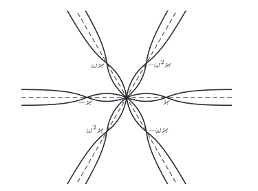
(a) Coutour $\hat{\Sigma}$ for $\zeta<0$.

Let $\chi_{\mathcal{Z}}\in C_{0}^{\infty}(\mathbb{C},[0,1])$ be supported near the discrete spectrum such that

$$\chi_{\mathcal{Z}}(z)=\begin{cases}1\quad\mbox{dist}(z,\mathcal{Z})\leq\rho/3,\\ 0\quad\mbox{dist}(z,\mathcal{Z})\geq 2\rho/3,\end{cases}$$ (3.5)

where

$$\rho=\min\{\underset{z,z^{\prime}\in\mathcal{Z}}{\min}|z-z^{\prime}|,\mbox{dist}(\mathcal{Z},\mathbb{R})\}.$$

Without loss of generality, we only consider jumps on the real axis and other case and other cases may be obtained by rotation.

Figure 3.1: the region $\Omega_{k}$

Lemma 3.2.

It is possible to define functions $R_{j}:\bar{\Omega}_{j}\to\mathbb{C},j=1,2,\dots,8$ with boundary values satisfying

$$R_{1}(z)=\begin{cases}-\frac{r(z)}{1-|r(z)|^{2}},\qquad\qquad\qquad\qquad\qquad\quad\,\,\,\,z\in(-\infty,\varkappa),\\ f_{1}=-\frac{\tilde{r}_{0}}{1-|\tilde{r}_{0}|^{2}}\frac{\delta_{+}^{2}(z)}{\delta(\omega^{2}z)\delta(\omega z)}(z+\varkappa)^{-2i\nu}(1-\chi_{\mathcal{Z}}(z)),\quad z\in\Sigma_{1},\end{cases}$$

$$R_{2}(z)=\begin{cases}\bar{r}(z),\qquad\qquad\qquad\qquad\qquad\qquad\qquad\,z\in(-\varkappa,0),\\ f_{2}=\tilde{r}_{0}\frac{\delta(\omega^{2}z)\delta(\omega z)}{\delta^{2}(z)}(z+\varkappa)^{2i\nu}(1-\chi_{\mathcal{Z}}(z))\quad\qquad\quad\,\,\,\,\,z\in\Sigma_{2},\end{cases}$$

$$R_{3}(z)=\begin{cases}\bar{r}(z),\qquad\qquad\qquad\qquad\qquad\qquad\qquad\,z\in(0,\varkappa),\\ f_{3}=\bar{r}_{0}\frac{\delta(\omega^{2}z)\delta(\omega z)}{\delta^{2}(z)}(z-\varkappa)^{2i\nu}(1-\chi_{\mathcal{Z}}(z))\quad\qquad\quad\,\,\,\,\,z\in\Sigma_{3},\end{cases}$$

$$R_{4}(z)=\begin{cases}-\frac{r(z)}{1-|r(z)|^{2}},\qquad\qquad\qquad\qquad\qquad\quad\,\,\,\,z\in(\varkappa,+\infty),\\ f_{4}=-\frac{\hat{r}_{0}}{1-|\hat{r}_{0}|^{2}}\frac{\delta_{+}^{2}(z)}{\delta(\omega^{2}z)\delta(\omega z)}(z-\varkappa)^{-2i\nu}(1-\chi_{\mathcal{Z}}(z))\quad\,\,\,z\in\Sigma_{4},\end{cases}$$

$$R_{5}(z)=\begin{cases}\frac{\bar{r}(z)}{1-|r(z)|^{2}},\quad\qquad\qquad\qquad\qquad\qquad\quad\,\,\,\,z\in(-\infty,\varkappa),\\ f_{5}=\frac{\tilde{r}_{0}}{1-|\tilde{r}_{0}|^{2}}\frac{\delta(\omega^{2}z)\delta(\omega z)}{\delta_{-}^{2}(z)}(z+\varkappa)^{2i\nu}(1-\chi_{\mathcal{Z}}(z))\qquad\quad z\in\Sigma_{5},\end{cases}$$

$$R_{6}(z)=\begin{cases}-r(z),\quad\qquad\qquad\qquad\qquad\qquad\qquad\,\,\,\,z\in(0,\varkappa),\\ f_{6}=-\tilde{r}_{0}\frac{\delta^{2}(z)}{\delta(\omega^{2}z)\delta(\omega z)}(z+\varkappa)^{-2i\nu}(1-\chi_{\mathcal{Z}}(z))\qquad\quad\,\,\,\,z\in\Sigma_{6},\end{cases}$$

$$R_{7}(z)=\begin{cases}-r(z),\quad\qquad\qquad\qquad\qquad\qquad\qquad\,\,\,\,z\in(0,\varkappa),\\ f_{7}=-\hat{r}_{0}\frac{\delta^{2}(z)}{\delta(\omega^{2}z)\delta(\omega z)}(z-\varkappa)^{-2i\nu}(1-\chi_{\mathcal{Z}}(z))\qquad\quad\,\,\,\,z\in\Sigma_{7},\end{cases}$$

$$R_{8}(z)=\begin{cases}\frac{\bar{r}(z)}{1-|r(z)|^{2}},\quad\qquad\qquad\qquad\qquad\qquad\quad\,\,\,\,z\in(\varkappa,+\infty),\\ f_{8}=\frac{\hat{r}_{0}}{1-|\hat{r}_{0}|^{2}}\frac{\delta(\omega^{2}z)\delta(\omega z)}{\delta_{-}^{2}(z)}(z-\varkappa)^{2i\nu}(1-\chi_{\mathcal{Z}}(z))\qquad\quad z\in\Sigma_{8},\end{cases}$$

where

$$\hat{r}_{0}=r(\varkappa)e^{-i\nu(-\varkappa)-i\nu(\varkappa)-i\beta_{1}(\varkappa,-\varkappa)+i\beta_{2}(\varkappa,\varkappa)}(2\varkappa)^{i\nu(-\varkappa)},$$

$$\tilde{r}_{0}=r(-\varkappa)e^{-i\nu(-\varkappa)-i\nu(\varkappa)-i\beta_{1}(-\varkappa,-\varkappa)+i\beta_{2}(-\varkappa,\varkappa)}(-2\varkappa)^{i\nu(\varkappa)}.$$

Lemma 3.3.

There exist function $R_{i}$ on $\Omega_{i}$ satisfying Lemma 3.2 so that

$$|\bar{\partial}R_{i}(z)|\lesssim|p^{\prime}(Re(z))|+|z\pm\varkappa|^{-1/2}+\bar{\partial}(\chi_{\mathcal{Z}}),$$ (3.6)

where the implied constant are uniform for $r$ in a bounded subset of $H^{1}$.

Proof.

We give the details firstly for $R_{4}(z)$:

$$R_{4}(z)=\Big{(}f_{4}+[-\frac{r(Rez)}{1-|r(Rez)|^{2}}-f_{4}(z)]\mathcal{K}(\phi)\Big{)}(1-\chi_{\mathcal{Z}}),$$

where $z=\varkappa+\rho e^{i\psi},\rho\geq 0,0\leq\psi\leq\arctan(\frac{0.2}{\varkappa-1.5})$, where $\phi=\arg(z-\varkappa)$ and $\mathcal{K}$ is a smooth function on $(0,\arctan(\frac{0.2}{\varkappa-1.5}))$,

$$\mathcal{K}(\phi)=\begin{cases}1,\quad z\in[0,\pi/20],\\ 0,\quad z\in[\pi/30,\pi/10].\end{cases}$$

We have

$$\bar{\partial}R_{4}(z) =\Big{(}\frac{1}{2}(-\frac{r(Rez)}{1-|r(Rez)|^{2}})^{\prime}\mathcal{K}(\phi)-\Big{[}-\frac{r(Rez)}{1-|r(Rez)|^{2}}-f_{4}(z)\Big{]}\frac{ie^{i\phi}}{|z-\varkappa|}\mathcal{K}^{\prime}(\phi)\Big{)}$$

$$\times(1-\chi_{\mathcal{Z}})-(f_{4}(z)+\Big{[}-\frac{r(Rez)}{1-|r(Rez)|^{2}}-f_{4}(z)\Big{]}\mathcal{K}(\phi))\bar{\partial}(\chi_{\mathcal{Z}}).$$

It follows that we acquire

$$|\bar{\partial}R_{4}(z)|\lesssim\Big{|}(-\frac{r(Rez)}{1-|r(Rez)|^{2}})^{\prime}\Big{|}+|z-\varkappa|^{-1/2}+\bar{\partial}(\chi_{\mathcal{Z}}).$$

Then we give the estimate for $R_{2}(z)$. The other cases are easily inferred. For $z\in\Omega_{3}$, we set

$$z=-\varkappa+re^{i\varphi}=(-\varkappa+r\cos\varphi)+ir\sin\varphi.$$

Then the continuous extension of $R_{2}(z)$ can be constructed by

$$R_{2}(z) =[h\bar{r}(z)+(1-h)f_{2}](1-\chi_{\mathcal{Z}}(z))$$

$$=f_{2}+h(\bar{r}(z)-f_{2})(1-\chi_{\mathcal{Z}}(z)),$$

where

$$h=h(r,\varphi)=\frac{d_{2}}{d_{1}+d_{2}},$$

where $d_{1,2}$ respectively represent the distance from $z$ to $(-\varkappa,0)$ and $\Sigma_{2}$, they are defined as

$$d_{1}=d_{1}(r,\varphi)=r\cos\varphi,$$

$$d_{2}=d_{2}(r,\varphi)=\min(\frac{1}{10}\sin\frac{\varkappa}{\pi}x-r\cos\varphi,\frac{0.2}{\varkappa-1.5}r\cos\varphi+\frac{0.2\varkappa}{\varkappa-1.5})$$

Finally, we have

$$|\bar{r}(z)(z+\varkappa)^{2i\nu}| =|\bar{r}(z)|e^{-2\nu\arg(z+\varkappa)}$$

$$\leq|\bar{r}(z|(1-|\bar{r}(z)|^{2}))^{-1}$$

$$\leq c_{1}+c_{2}|1+z^{2}|^{-\frac{1}{4}}.$$

Utilizing $\bar{\partial}=\frac{1}{2}e^{i\varphi}(\partial_{r}+ir^{-1}\partial_{\varphi})$, we have

$$\bar{\partial}R_{2}(z) =-[f_{2}+h(\bar{r}(z)-f_{2})]\bar{\partial}\chi_{\mathcal{Z}}(z)$$

$$+\frac{1}{2}e^{i\varphi}(h_{r}+ir^{-1}h_{\varphi})(\bar{r}(z)-f_{2})(1-\chi_{\mathcal{Z}}(z)),$$

and

$$|\bar{\partial}R_{11}(z)|\leq c_{1}|\bar{\partial}\chi_{\mathcal{Z}}(z)|+c_{2}|\bar{(}z)-f_{2}|+c_{3}\frac{|\bar{r}(z)-f_{2}|}{|z+\varkappa|},$$

which acquire the estimate of (3.6). ∎

We use the extension in Lemma 3.2 to define a new unknown function

$$M^{(2)}_{\oplus}(y,t,z)=M_{\oplus}(y,t,z)\mathcal{R}^{(2)}(z),$$ (3.7)

$$\mathcal{R}^{(2)}=\begin{cases}\begin{pmatrix}1&0&0\\ R_{1}\frac{\delta(\omega^{2}z)\delta(\omega z)}{\delta_{+}^{2}(z)}e^{2it\theta}&1&0\\ 0&0&1\end{pmatrix}^{-1},\quad z\in\Omega_{1},\quad\begin{pmatrix}1&R_{2}\frac{\delta^{2}(z)}{\delta(\omega^{2}z)\delta(\omega z)}e^{-2it\theta}&0\\ 0&1&0\\ 0&0&1\end{pmatrix}^{-1},\quad z\in\Omega_{2},\\ \\ \begin{pmatrix}1&R_{3}\frac{\delta^{2}(z)}{\delta(\omega^{2}z)\delta(\omega z)}e^{-2it\theta}&0\\ 0&1&0\\ 0&0&1\end{pmatrix}^{-1},\quad z\in\Omega_{3},\quad\begin{pmatrix}1&0&0\\ R_{4}\frac{\delta(\omega^{2}z)\delta(\omega z)}{\delta_{+}^{2}(z)}e^{2it\theta}&1&0\\ 0&0&1\end{pmatrix}^{-1},\quad z\in\Omega_{4},\\ \\ \begin{pmatrix}1&R_{5}\frac{\delta_{-}^{2}(z)}{\delta(\omega^{2}z)\delta(\omega z)}e^{-2it\theta}&0\\ 0&1&0\\ 0&0&1\end{pmatrix},\qquad z\in\Omega_{5},\quad\begin{pmatrix}1&0&0\\ R_{6}\frac{\delta(\omega^{2}z)\delta(\omega z)}{\delta^{2}(z)}e^{2it\theta}&1&0\\ 0&0&1\end{pmatrix},\qquad z\in\Omega_{6},\\ \\ \begin{pmatrix}1&0&0\\ R_{7}\frac{\delta(\omega^{2}z)\delta(\omega z)}{\delta^{2}(z)}e^{2it\theta}&1&0\\ 0&0&1\end{pmatrix},\qquad z\in\Omega_{7},\qquad\begin{pmatrix}1&R_{8}\frac{\delta_{-}^{2}(z)}{\delta(\omega^{2}z)\delta(\omega z)}e^{-2it\theta}&0\\ 0&1&0\\ 0&0&1\end{pmatrix},\qquad z\in\Omega_{8},\\ \\ \begin{pmatrix}1&0&0\\ 0&1&0\\ 0&0&1\end{pmatrix},\qquad z\in(\Omega_{9}\cup\Omega_{10}).\end{cases}$$

satisfies the following $\bar{\partial}-$RH problem.

RHP 3.3.

Find a continuous with sectionally continuous first partial derivatives function $M^{(2)}_{\oplus}(y,t,z):\mathbb{C}\setminus(\hat{\Sigma}\cup\Gamma)\to$SL${}_{3}(\mathbb{C})$ with the following properties:

$\bigstar$(the normalization condition)

$$M^{(2)}_{\oplus}(y,t,z)=I+\mathcal{O}(z^{-1})\quad z\to\infty.$$

$\bigstar$(the jump condition)

For each $z\in\hat{\Sigma}$, the boundary values $M^{(2)}_{\oplus}(y,t,z)$ satisfy the jump relation $M^{(2+)}_{\oplus}(y,t,z)=M^{(2-)}_{\oplus}(y,t,z)S^{(2)}_{\oplus}(y,t,z),\,\,y\in\hat{\Sigma}$ where the jump matrix

$$S^{(2)}_{\oplus}(y,t,z)=\begin{cases}\begin{pmatrix}1&0&0\\ R_{1}\frac{\delta(\omega^{2}z)\delta(\omega z)}{\delta_{+}^{2}(z)}e^{2it\theta}&1&0\\ 0&0&1\end{pmatrix},\quad z\in\Sigma_{1}\quad\begin{pmatrix}1&R_{2}\frac{\delta^{2}(z)}{\delta(\omega^{2}z)\delta(\omega z)}e^{-2it\theta}&0\\ 0&1&0\\ 0&0&1\end{pmatrix},\quad z\in\Sigma_{2}\\ \\ \begin{pmatrix}1&R_{3}\frac{\delta^{2}(z)}{\delta(\omega^{2}z)\delta(\omega z)}e^{-2it\theta}&0\\ 0&1&0\\ 0&0&1\end{pmatrix},\quad z\in\Sigma_{3}\quad\begin{pmatrix}1&0&0\\ R_{4}\frac{\delta(\omega^{2}z)\delta(\omega z)}{\delta_{+}^{2}(z)}e^{2it\theta}&1&0\\ 0&0&1\end{pmatrix},\quad z\in\Sigma_{4}\\ \\ \begin{pmatrix}1&R_{5}\frac{\delta_{-}^{2}(z)}{\delta(\omega^{2}z)\delta(\omega z)}e^{-2it\theta}&0\\ 0&1&0\\ 0&0&1\end{pmatrix},\quad z\in\Sigma_{5}\quad\begin{pmatrix}1&0&0\\ R_{6}\frac{\delta(\omega^{2}z)\delta(\omega z)}{\delta^{2}(z)}e^{2it\theta}&1&0\\ 0&0&1\end{pmatrix}\quad z\in\Sigma_{6}\\ \\ \begin{pmatrix}1&0&0\\ R_{7}\frac{\delta(\omega^{2}z)\delta(\omega z)}{\delta^{2}(z)}e^{2it\theta}&1&0\\ 0&0&1\end{pmatrix},z\in\Sigma_{7}quad\begin{pmatrix}1&R_{8}\frac{\delta_{-}^{2}(z)}{\delta(\omega^{2}z)\delta(\omega z)}e^{-2it\theta}&0\\ 0&1&0\\ 0&0&1\end{pmatrix},\quad z\in\Sigma_{8}\end{cases}$$ (3.8)

$\bigstar$(the residue condition)

The residue condition of $M^{(2)}_{\oplus}(y,t,z)$ is as same as $M_{\Diamond}(y,t,z)$ of RH problem 2.1.

$\bigstar$(Singularities)

As $z\to 0$, the limit of $M^{(2)}_{\oplus}(y,t,z)$ has pole singularities as $M_{\Diamond}(y,t,z)$.

$\bigstar$($\bar{\partial}$ about the jump matrix)

$$\bar{\partial}S^{(2)}(y,t;z)=\begin{cases}\begin{pmatrix}1&0&0\\ \bar{\partial}R_{1}\frac{\delta(\omega^{2}z)\delta(\omega z)}{\delta_{+}^{2}(z)}e^{2it\theta}&1&0\\ 0&0&1\end{pmatrix},\quad z\in\Sigma_{1}\quad\begin{pmatrix}1&\bar{\partial}R_{2}\frac{\delta^{2}(z)}{\delta(\omega^{2}z)\delta(\omega z)}e^{-2it\theta}&0\\ 0&1&0\\ 0&0&1\end{pmatrix},\quad z\in\Sigma_{2}\\ \\ \begin{pmatrix}1&\bar{\partial}R_{3}\frac{\delta^{2}(z)}{\delta(\omega^{2}z)\delta(\omega z)}e^{-2it\theta}&0\\ 0&1&0\\ 0&0&1\end{pmatrix},\quad z\in\Sigma_{3}\quad\begin{pmatrix}1&0&0\\ \bar{\partial}R_{4}\frac{\delta(\omega^{2}z)\delta(\omega z)}{\delta_{+}^{2}(z)}e^{2it\theta}&1&0\\ 0&0&1\end{pmatrix},\quad z\in\Sigma_{4}\\ \\ \begin{pmatrix}1&\bar{\partial}R_{5}\frac{\delta_{-}^{2}(z)}{\delta(\omega^{2}z)\delta(\omega z)}e^{-2it\theta}&0\\ 0&1&0\\ 0&0&1\end{pmatrix},\quad z\in\Sigma_{5}\quad\begin{pmatrix}1&0&0\\ \bar{\partial}R_{6}\frac{\delta(\omega^{2}z)\delta(\omega z)}{\delta^{2}(z)}e^{2it\theta}&1&0\\ 0&0&1\end{pmatrix}\quad z\in\Sigma_{6}\\ \\ \begin{pmatrix}1&0&0\\ \bar{\partial}R_{7}\frac{\delta(\omega^{2}z)\delta(\omega z)}{\delta^{2}(z)}e^{2it\theta}&1&0\\ 0&0&1\end{pmatrix},z\in\Sigma_{7}\qquad\,\,\,\begin{pmatrix}1&\bar{\partial}R_{8}\frac{\delta_{-}^{2}(z)}{\delta(\omega^{2}z)\delta(\omega z)}e^{-2it\theta}&0\\ 0&1&0\\ 0&0&1\end{pmatrix},\quad z\in\Sigma_{8}\end{cases}$$ (3.9)

Remark 3.4.

In the $\bar{\partial}$-RH problem 3.3, it is useful to recall how the extensions $R_{j}(z)$ are defined in Lemma 3.2, particularly in Lemma 3.3. Through the $\bar{\partial}$ of $M^{(2)}_{\oplus}(y,t,z)$ may seem to that $M^{(2)}_{\oplus}(y,t,z)$ is non-analytic near points the discrete spectrum, the $\bar{\partial}$-derivative vanishes in small neighborhoods of each point of the discrete spectrum so that $M^{(2)}_{\oplus}(y,t,z)$ is analytic in each neighborhood.

3.3 Analysis on the pure RH problem

In this section we build a solution $M_{rhp}^{(2)}(z)$ to the RH problem that results from RH problem 3.3 for $M^{(2)}_{\oplus}(y,t,z)$ by dropping the $\bar{\partial}$ component. Specifically: Let $M_{rhp}^{(2)}(z)$ be the solution of the RH problem 3.3 resulting from stetting $\bar{\partial}\mathcal{R}^{(2)}=0$. We perform the following factorization of $M^{(2)}_{\oplus}(y,t,z)$:

$$M^{(2)}_{\oplus}(y,t,z)=M^{(3)}(z)M_{rhp}^{(2)}(z),$$ (3.10)

where $M^{(3)}(z)$ is a continuously differentiable function satisfying the following $\bar{\partial}$-problem 3.1.

$\bar{\partial}$-RHP 3.1.

Find a continuous with sectionally continuous first partial derivatives function $M^{(3)}(z):\mathbb{C}\to SL_{3}(\mathbb{C})$ with the following properties:

$\bigstar$(the normalization condition)

$$M^{(3)}(z)=I+\mathcal{O}(z^{-1})\quad z\to\infty.$$

$\bigstar$(the $\bar{\partial}$ condition)

For $z\in\mathbb{C}$, we have

$$\bar{\partial}M^{(3)}(z)=M^{(3)}(z)W^{(3)}(z),$$ (3.11)

where $W^{(3)}(z):=M_{rhp}^{(2)}(z)\bar{\partial}\mathcal{R}^{(2)}(z)M_{rhp}^{(2)}(z)^{-1}$.

In this section focuses on find $M_{rhp}^{(2)}(z)$ which is meromorphic away from the contour $\hat{\Sigma}$ on which its boundary values satisfy the jump relation (3.8).

RHP 3.4.

Find an analytic function $M_{rhp}^{(2)}(z):\mathbb{C}\setminus\hat{\Sigma}_{r}\to SL_{3}(\mathbb{C})$ such that

$\bigstar$(the normalization condition)

$$M_{rhp}^{(2)}(z)=I+\mathcal{O}(z^{-1})\quad z\to\infty.$$

$\bigstar$(the jump condition)

For $z\in\mathbb{C}\setminus\hat{\Sigma}_{r}$, we have the jump relation $M_{rhp}^{(2)^{+}}(z)=M_{rhp}^{(2)^{-}}(z)V^{(2)}_{rhp}(z)$, where

$$V^{(2)}_{rhp}(z)=S^{(2)}_{\oplus}(y,t,z)|_{\Sigma_{r}}.$$

Figure 3.2: $\hat{\Sigma}=\hat{\Sigma}_{b}\cup\hat{\Sigma}_{r}$, where $\hat{\Sigma}_{b}$ and $\hat{\Sigma}_{r}$ are respectively the black and red portion of $\hat{\Sigma}$ and $\hat{\Sigma}_{b}=\hat{\Sigma}_{l}\cup\hat{\Sigma}_{r}$

Now we decompose $W^{(2)}=V^{(2)}_{rhp}(z)-I$ into two parts:

$$W^{(2)}=W^{e}+W^{\prime},$$ (3.12)

where $W^{\prime}=W^{(2)}|_{\hat{\Sigma}_{b}}$ and $W^{e}=W^{(2)}|_{\hat{\Sigma}_{r}}$. on $\hat{\Sigma}_{l}$ away from $-\varkappa$, we estimate:

$$|R_{1}e^{2it\theta}|\leq C_{r}e^{-\frac{1}{2}\epsilon^{2}t}, |R_{2}e^{-2it\theta}|\leq C_{r}e^{-\frac{1}{2}\epsilon^{2}t},$$

$$|R_{5}e^{-2it\theta}|\leq C_{r}e^{-\frac{1}{2}\epsilon^{2}t}, |R_{6}e^{2it\theta}|\leq C_{r}e^{-\frac{1}{2}\epsilon^{2}t},$$

and on $\hat{\Sigma}_{r}$ away from $\varkappa$, we estimate:

$$|R_{3}e^{-2it\theta}|\leq C_{r}e^{-\frac{1}{2}\epsilon^{2}t}, |R_{4}e^{2it\theta}|\leq C_{r}e^{-\frac{1}{2}\epsilon^{2}t},$$

$$|R_{7}e^{2it\theta}|\leq C_{r}e^{-\frac{1}{2}\epsilon^{2}t}, |R_{8}e^{-2it\theta}|\leq C_{r}e^{-\frac{1}{2}\epsilon^{2}t},$$

with the discussion above we conclude that

$$\big{|}W^{e}\big{|}\lesssim e^{-ct}.$$ (3.13)

Proposition 3.5.

There exists a 2$\times$2 matrix $E_{1}(z)$ with

$$E_{1}(z)=I+\mathcal{O}\big{(}\frac{e^{-ct}}{z}\big{)},$$ (3.14)

such that

$$M_{rhp}^{(2)}(z)=E_{1}(z)M_{rhp}^{(2)^{*}}(z),$$ (3.15)

where $M_{rhp}^{(2)^{*}}(z)$ solves the RH problem 3.5 and 3.8 with jump contour $\Sigma_{r}$ and $\Sigma_{l}$.

Proof.

We will later show the existence of $M_{rhp}^{(2)^{*}}(z)$ and $\big{\|}M_{rhp}^{(2)^{*}}(z)\big{\|}_{L^{\infty}}$ is finite. Assuming that, it is easy to see that on $\hat{\Sigma}^{(2)}\setminus(\hat{\Sigma}^{(2)}_{r}\cup\hat{\Sigma}^{(2)}_{l})$, $E_{1}$ satisfies the following jump condition:

$$E_{1+}=E_{1-}\big{(}M_{rhp}^{(2)^{*}}(z)(I+W^{e})\big{(}M_{*}^{LC}\big{)}^{-1}\big{)}.$$

Using (3.13) the conclusion follows from solving a small norm RH problem 3.5 and 3.8 see below. ∎

3.3.1 A local model near the saddle point

RHP 3.5.

Find a 3$\times$3 matrix-valued function $\mathbf{M_{r}}(z)$, analytic on $\mathbb{C}\setminus\hat{\Sigma}_{r}$, with the following properties:

$\bigstar$(the normalization condition)

$$\mathbf{M_{r}}(z)=I+\mathcal{O}(z^{-1}),\quad z\to\infty.$$

$\bigstar$(the jump condition)

$\mathbf{M_{r}}(z)$ is continuous boundary value $\mathbf{M_{r}}^{\pm}(z)$ on $\hat{\Sigma}_{r}$, we have the jump relation $\mathbf{M_{r}}^{+}(z)=\mathbf{M_{r}}^{-}(z)\mathbf{V_{r}}(z)$, where

$$\mathbf{V_{r}}(z)=S^{(2)}_{\oplus}(y,t,z)|_{\Sigma_{r}}..$$

Now set

$$\zeta(z)=\sqrt{ct}(z-\varkappa),\quad c=\frac{2\sqrt{3}}{\varkappa^{3}}.$$ (3.16)

and

$$r_{\xi}=\hat{r}_{0}e^{-\frac{\sqrt{3}}{\varkappa}t}\Big{(}\frac{8\sqrt{3}}{\varkappa}t\Big{)}^{-i\nu/2}.$$ (3.17)

Under the change of variables (3.38), the phase $e^{2it\theta}$ identifies to $e^{-i\zeta^{2}/2}e^{-i\sqrt{3}t/\varkappa}$. The factor $e^{-i\zeta^{2}/2}$ will be following important in the identification of parabolic cylinder functions.

RHP 3.6.

Find a 3$\times$3 matrix-valued function $\mathbf{N^{PC}}(z)$, analytic on $\mathbb{C}\setminus\hat{\Sigma}_{r}$, with the following properties:

$\bigstar$(the normalization condition)

$$\mathbf{N^{PC}}(z)=I+\mathcal{O}(z^{-1})\quad z\to\infty$$

$\bigstar$(the jump condition)

$\mathbf{N^{PC}}(z)$ is continuous boundary value $\mathbf{N^{PC}}^{\pm}(z)$ on $\hat{\Sigma}_{r}$, we have the jump relation $\mathbf{N^{PC}}^{+}(z)=\mathbf{N^{PC}}^{-}(z)\mathbf{V^{(PC)}}(z)$, where

$$\mathbf{V^{(PC)}}(z)=S^{(2)}_{\oplus}(y,t,z)|_{\hat{\Sigma}_{r}}$$

where

$$\mathbf{V^{(PC)}}(z)=\begin{cases}\begin{pmatrix}1&r_{\xi}(-\zeta)^{2i\nu}e^{-i\nu^{2}/2}&0\\ 0&1&0\\ 0&0&1\end{pmatrix},\qquad\quad z\in\Sigma_{3},\\ \\ \begin{pmatrix}1&0&0\\ -\frac{r_{\xi}}{1-|r_{\xi}|^{2}}(-\zeta)^{2i\nu}e^{-i\nu^{2}/2}&1&0\\ 0&0&1\end{pmatrix},\quad z\in\Sigma_{4},\\ \\ \begin{pmatrix}1&0&0\\ -r_{\xi}(-\zeta)^{2i\nu}e^{-i\nu^{2}/2}&1&0\\ 0&0&1\end{pmatrix},\qquad\quad z\in\Sigma_{7},\\ \\ \begin{pmatrix}1&\frac{r_{\xi}}{1-|r_{\xi}|^{2}}(-\zeta)^{2i\nu}e^{-i\nu^{2}/2}&0\\ 0&1&0\\ 0&0&1\end{pmatrix},\qquad z\in\Sigma_{8}.\\ \end{cases}$$ (3.18)

It is possible to further reduce the RH problem 3.6 to a model RH problem 3$\times$3 matrix solution is piecewise analytic in the upper and lower complex plane. In each half-plane, the entries of the matrix satisfy ODEs that are obtained from analytic properties as well as the large $\zeta$ behavior. The solution of the ODEs are explicitly calculated in terms of parabolic cylinder functions. Let

$$\mathbf{N^{PC}}(\xi,\zeta)=\Phi(\xi,\zeta)\mathcal{P}(\xi)\begin{pmatrix}e^{i\nu^{2}/4}&0&0\\ 0&e^{-i\nu^{2}/4}&0\\ 0&0&1\end{pmatrix}\begin{pmatrix}(-\zeta)^{-i\nu}&0&0\\ 0&(-\zeta)^{i\nu}&0\\ 0&0&1\end{pmatrix},$$ (3.19)

where

$$\mathbf{V^{(PC)}}(z)=\begin{cases}\begin{pmatrix}1&r_{\xi}&0\\ 0&1&0\\ 0&0&1\end{pmatrix},\quad z\in\Omega_{3},\qquad\begin{pmatrix}1&0&0\\ -\frac{r_{\xi}}{1-|r_{\xi}|^{2}}&1&0\\ 0&0&1\end{pmatrix},\quad z\in\Omega_{4},\\ \\ \begin{pmatrix}1&0&0\\ -r_{\xi}&1&0\\ 0&0&1\end{pmatrix},\quad z\in\Omega_{7},\quad\,\begin{pmatrix}1&\frac{r_{\xi}}{1-|r_{\xi}|^{2}}&0\\ 0&1&0\\ 0&0&1\end{pmatrix},\quad z\in\Omega_{8},\\ \\ \begin{pmatrix}1&0&0\\ 0&1&0\\ 0&0&1\end{pmatrix},\quad z\in\Omega_{9}\cup\Omega_{10}.\end{cases}$$ (3.20)

By construction, the matrix $\Phi$ is continuous along the rays of $\hat{\Sigma}_{r}$. Let us set up the RH problem it satisfies and compute its jumps along the real axis. We have along the real axis

$$\Phi_{+}=\Phi_{-}\Bigg{\{}\mathcal{P}\begin{pmatrix}e^{i\nu^{2}/4}&0&0\\ 0&e^{-i\nu^{2}/4}&0\\ 0&0&1\end{pmatrix}\begin{pmatrix}(-\zeta)^{-i\nu}&0&0\\ 0&(-\zeta)^{i\nu}&0\\ 0&0&1\end{pmatrix}\Bigg{\}}_{-}$$ (3.21)

$$\Bigg{\{}\begin{pmatrix}e^{-i\nu^{2}/4}&0&0\\ 0&e^{i\nu^{2}/4}&0\\ 0&0&1\end{pmatrix}\begin{pmatrix}(-\zeta)^{i\nu}&0&0\\ 0&(-\zeta)^{-i\nu}&0\\ 0&0&1\end{pmatrix}\mathcal{P}^{-1}\Bigg{\}}_{+}.$$ (3.22)

Due to the branch cut of the logarithmic function along the $(-\infty,-\varkappa)\cup(\varkappa,+\infty)$, we have along the negative real axis,

$$\begin{pmatrix}(-\zeta)^{-i\nu}&0&0\\ 0&(-\zeta)^{i\nu}&0\\ 0&0&1\end{pmatrix}_{-}\begin{pmatrix}(-\zeta)^{i\nu}&0&0\\ 0&(-\zeta)^{-i\nu}&0\\ 0&0&1\end{pmatrix}_{+}=\begin{pmatrix}e^{-2\nu\pi}&0&0\\ 0&e^{2\nu\pi}&0\\ 0&0&1\end{pmatrix}.$$

while along the $(-\varkappa,\varkappa)$

$$\begin{pmatrix}(-\zeta)^{-i\nu}&0&0\\ 0&(-\zeta)^{i\nu}&0\\ 0&0&1\end{pmatrix}_{-}\begin{pmatrix}(-\zeta)^{i\nu}&0&0\\ 0&(-\zeta)^{-i\nu}&0\\ 0&0&1\end{pmatrix}_{+}=I.$$

This implies that the matrix $\Phi$ has the same (constant) jump matrix along the

$$V^{(0)}=\begin{pmatrix}1&\bar{r}_{\xi}(z)&0\\ -r_{\xi}(z)&1-|r_{\xi}(z)|^{2}&0\\ 0&0&1\end{pmatrix}.$$ (3.23)

and the 3$\times$3 matrix $\Phi$ satisfies the following model RH problem 3.7.

RHP 3.7.

Find a 3$\times$3 matrix-valued function $\Phi(z;\xi)$, analytic on $\mathbb{C}\setminus\mathbb{R}$, with the following properties:

$\bigstar$(the boundary value condition)

$$\Phi(z)\sim\begin{pmatrix}e^{-i\nu^{2}/4}&0&0\\ 0&e^{i\nu^{2}/4}&0\\ 0&0&1\end{pmatrix}\begin{pmatrix}(-\zeta)^{i\nu}&0&0\\ 0&(-\zeta)^{-i\nu}&0\\ 0&0&1\end{pmatrix}\quad z\to\infty\quad\mbox{in}\quad\mathbb{C}\setminus\mathbb{R}.$$

$\bigstar$(the jump condition) $\Phi(z)$ is analytic for $z\in\mathbb{C}\setminus\mathbb{R}$ with continuous boundary values $\Phi_{\pm}$ on $\mathbb{R}$ with the jump relation

$$\Phi_{+}(z)=\Phi_{-}(z)V^{(0)}.$$ (3.24)

Differentiating (3.24) with respect to $\zeta$, we obtain that

$$\Bigg{(}\frac{d\Phi}{d\zeta}+\begin{pmatrix}\frac{1}{2}i\zeta&0&0\\ 0&-\frac{1}{2}i\zeta&0\\ 0&0&1\end{pmatrix}\Phi\Bigg{)}_{+}=\Bigg{(}\frac{d\Phi}{d\zeta}+\begin{pmatrix}\frac{1}{2}i\zeta&0&0\\ 0&-\frac{1}{2}i\zeta&0\\ 0&0&1\end{pmatrix}\Phi\Bigg{)}_{-}V^{(0)}.$$

We know that $\det V^{(0)}=1$, thus $\det\Phi_{+}=\det\Phi_{-}$ and $\det\Phi$ is analytic in the whole complex plane. It is equal to one at infinity, thus by Liouville theorem, $\det\Phi=1$. It follows that $(\Phi)^{-1}$ exists and it bounded. The matrix

$$\Bigg{(}\frac{d\Phi}{d\zeta}+\begin{pmatrix}\frac{1}{2}i\zeta&0&0\\ 0&-\frac{1}{2}i\zeta&0\\ 0&0&1\end{pmatrix}\Phi\Bigg{)}\Phi^{-1},$$

has no jump along the real line and is therefore an entire function of $\zeta$. According to (3.19), we have that

$$\Bigg{(}\frac{d\Phi}{d\zeta}+\begin{pmatrix}\frac{1}{2}i\zeta&0&0\\ 0&-\frac{1}{2}i\zeta&0\\ 0&0&1\end{pmatrix}\Phi\Bigg{)}\Phi^{-1}=\Bigg{(}\frac{\mathbf{N^{PC}}(z)}{d\zeta}+\frac{\mathbf{N^{PC}}(z)}{\zeta}\begin{pmatrix}i\nu&0&0\\ 0&-i\nu&0\\ 0&0&1\end{pmatrix}\Bigg{)}\mathbf{N^{PC}}(z)^{-1}$$

$$+\Bigg{\{}\begin{pmatrix}\frac{i\zeta}{2}&0&0\\ 0&-\frac{i\zeta}{2}&0\\ 0&0&1\end{pmatrix}\mathbf{N^{PC}}(z)-\mathbf{N^{PC}}(z)\begin{pmatrix}\frac{i\zeta}{2}&0&0\\ 0&-\frac{i\zeta}{2}&0\\ 0&0&1\end{pmatrix}\Bigg{\}}\mathbf{N^{PC}}(z)^{-1}.$$ (3.25)

The first term in the right hand side of (3.25) tends to $0$ as $\zeta\to\infty$ while the second term behaves like $\mathcal{O}(1/\zeta)$. For the last term in the right-hand side of (3.25), we use that

$$\mathbf{N^{PC}}(z)\sim(I+\frac{m^{(0)}}{\zeta}).$$ (3.26)

Defining

$$\beta =\begin{pmatrix}\frac{i}{2}&0&0\\ 0&-\frac{i}{2}&0\\ 0&0&1\end{pmatrix}\mathbf{N^{PC}}(z)-\mathbf{N^{PC}}(z)\begin{pmatrix}\frac{i}{2}&0&0\\ 0&-\frac{i}{2}&0\\ 0&0&1\end{pmatrix}$$ (3.27)

$$=\begin{pmatrix}0&im_{12}&0\\ -im_{21}&0&0\\ 0&0&0\end{pmatrix}.$$ (3.28)

Equivalently, $\beta_{12}=im_{12},\beta_{21}=-im_{21}$. Again applying Liouville’s theorem, the $3\times 3$ matrix $\Phi$ satisfies the ODE:

$$\frac{d\Phi}{d\zeta}+\begin{pmatrix}\frac{i\zeta}{2}&0&0\\ 0&-\frac{i\zeta}{2}&0\\ 0&0&1\end{pmatrix}\Phi=\beta\Phi,$$ (3.29)

where $\beta$ is an off-diagonal matrix.

The system (3.29) decouples into two first-order systems for $(\Phi_{11},\Phi_{21},\Phi_{31})$, $(\Phi_{12},\Phi_{22},\Phi_{32})$ and $(\Phi_{13},\Phi_{23},\Phi_{33})$,

$$\begin{cases}\frac{d\Phi_{11}}{d\zeta}+\frac{i\zeta}{2}\Phi_{11}=\beta_{12}\Phi_{21},\\ \frac{d\Phi_{21}}{d\zeta}-\frac{i\zeta}{2}\Phi_{21}=\beta_{21}\Phi_{11},\end{cases}$$ (3.30)

and

$$\begin{cases}\frac{d\Phi_{12}}{d\zeta}+\frac{i\zeta}{2}\Phi_{12}=\beta_{12}\Phi_{22},\\ \frac{d\Phi_{22}}{d\zeta}-\frac{i\zeta}{2}\Phi_{22}=\beta_{21}\Phi_{12},\end{cases}$$ (3.31)

and

$$\begin{cases}\frac{d\Phi_{13}}{d\zeta}+\frac{i\zeta}{2}\Phi_{13}=\beta_{12}\Phi_{23},\\ \frac{d\Phi_{23}}{d\zeta}-\frac{i\zeta}{2}\Phi_{23}=\beta_{21}\Phi_{13}.\end{cases}$$ (3.32)

Combining the above equations, one obtains that the entries of $\Phi$ satisfy following Lemma 3.6.

Lemma 3.6.

The entries of $\Phi$ obey the differential equations

$$\Phi_{11}^{{}^{\prime\prime}}+\Big{(}\frac{\zeta^{2}}{4}-(\beta_{12}\beta_{21})\Phi_{11}+\frac{i}{2}\Big{)}\Phi_{11}=0,$$

$$\Phi_{21}^{{}^{\prime\prime}}+\Big{(}\frac{\zeta^{2}}{4}-(\beta_{12}\beta_{21})\Phi_{21}-\frac{i}{2}\Big{)}\Phi_{21}=0,$$

$$\Phi_{12}^{{}^{\prime\prime}}+\Big{(}\frac{\zeta^{2}}{4}-(\beta_{12}\beta_{21})\Phi_{12}+\frac{i}{2}\Big{)}\Phi_{12}=0,$$

$$\Phi_{22}^{{}^{\prime\prime}}+\Big{(}\frac{\zeta^{2}}{4}-(\beta_{12}\beta_{21})\Phi_{21}-\frac{i}{2}\Big{)}\Phi_{22}=0,$$

$$\Phi_{13}^{{}^{\prime\prime}}+\Big{(}\frac{\zeta^{2}}{4}-(\beta_{12}\beta_{21})\Phi_{13}+\frac{i}{2}\Big{)}\Phi_{13}=0,$$

$$\Phi_{23}^{{}^{\prime\prime}}+\Big{(}\frac{\zeta^{2}}{4}-(\beta_{12}\beta_{21})\Phi_{23}-\frac{i}{2}\Big{)}\Phi_{23}=0.$$

The next step is to complement the ODEs with additional conditions taking into account the conditions at infinity as well as the jump conditions of $\Phi$. This will determine $\Phi$ uniquely and will identify the coefficients $\beta_{12},\beta_{21}$. The parabolic cylinder equation is

$$y^{\prime\prime}+(-\frac{z^{2}}{4}+a+\frac{1}{2})y=0.$$ (3.33)

The parabolic cylinder functions $D_{a}(z),D_{a}(-z),D_{-a-1}(iz),D_{-a-1}(-iz)$ all satisfy (3.33) and are entire for all any value $a$.
The large-$z$ behavior of $D_{a}(z)$ is given by the following formulas

$$D_{a}(z)\sim\begin{cases}z^{a}e^{-z^{2}/4},\qquad\qquad\qquad\qquad\qquad\qquad|\arg(z)|<\frac{3\pi}{4},\\ z^{a}e^{-z^{2}/4}-\frac{\sqrt{2\pi}}{\Gamma(-a)}e^{ia\pi}z^{-a-1}e^{z^{2}/4},\qquad\frac{\pi}{4}<\arg(z)<\frac{5\pi}{4},\\ z^{a}e^{-z^{2}/4}-\frac{\sqrt{2\pi}}{\Gamma(-a)}e^{-ia\pi}z^{-a-1}e^{z^{2}/4},\quad-\frac{5\pi}{4}<\arg(z)<-\frac{\pi}{4}.\end{cases}$$ (3.34)

Proposition 3.7.

The unique solution to RH Problem 3.7 is given by

$$\Phi(\zeta,r)=\begin{cases}\begin{pmatrix}e^{-\frac{3\pi\nu}{4}}D_{i\nu}(e^{-\frac{3i\pi}{4}}\zeta)&-\beta_{12}e^{\frac{\pi}{4}(\nu-i)}D_{-i\nu-1}(e^{-\frac{i\pi}{4}}\zeta)&0\\ i\beta_{21}e^{-\frac{3\pi}{4}(\nu+i)}D_{i\nu-1}(e^{-\frac{3i\pi}{4}}\zeta)&e^{\frac{\pi\nu}{4}}D_{-i\nu}(e^{-\frac{i\pi}{4}\zeta})&0\\ 0&0&1\end{pmatrix},\quad\zeta\in\mathbb{C}^{+},\\ \\ \begin{pmatrix}e^{\frac{\pi\nu}{4}}D_{i\nu}(e^{\frac{i\pi}{4}\zeta})&-\beta_{12}e^{-\frac{3\pi}{4}(\nu-i)}D_{-i\nu-1}(e^{\frac{3i\pi}{4}}\zeta)&0\\ i\beta_{21}e^{\frac{\pi}{4}(\nu+i)}D_{i\nu-1}(e^{\frac{i\pi}{4}}\zeta)&e^{-\frac{3\pi\nu}{4}}D_{-i\nu}(e^{\frac{3i\pi}{4}}\zeta)&0\\ 0&0&1\end{pmatrix},\quad\quad\,\,\zeta\in\mathbb{C}^{-}.\\ \end{cases}$$

We now impose the jump conditions to find the coefficients $\beta_{12}$ and $\beta_{21}$, we know that $\beta_{12}\beta_{21}=\nu$, we acquire

$$(\Phi_{-})^{-1}\Phi_{+}=V^{(0)}=\begin{pmatrix}1&\bar{r}_{\xi}(z)&0\\ -r_{\xi}(z)&1-|r_{\xi}(z)|^{2}&0\\ 0&0&1\end{pmatrix},$$

we obtain

$$-r_{\xi} =\Phi^{-}_{11}\Phi^{+}_{21}-\Phi^{-}_{21}\Phi^{+}_{11}$$

$$=e^{\frac{\pi}{4}\nu}D_{i\nu}(e^{i\pi/4}\zeta)\frac{1}{\beta_{12}}e^{-\frac{3\pi}{4}\nu}\Big{(}\partial_{\zeta}(D_{i\nu}(\zeta e^{-3i\pi/4}))+\frac{i\zeta}{2}D_{i\nu}(\zeta e^{-3i\pi/4})\Big{)}$$

$$\times\frac{e^{\frac{-\pi\nu}{2}}}{\beta_{12}}Wr\Big{(}D_{i\nu}(e^{i\pi/4}\zeta),D_{i\nu}(\varsigma e^{-3i\pi/4})\Big{)}$$

$$=\frac{\sqrt{2\pi}e^{-\frac{\pi\nu}{2}e^{i\pi/4}}}{\beta_{12}\Gamma(-i\nu)},$$

we obtain that $\beta_{12}$ and $\beta_{21}$ are the complex constants

$$\beta_{12}=-\frac{\sqrt{2\pi}e^{i\pi/4}e^{-\pi\nu/2}}{-r_{\xi}\Gamma(-i\nu)},$$

$$\beta_{21}=\frac{r_{\xi}\Gamma(i\nu)}{\sqrt{2\pi}e^{-i\pi/4}e^{-\pi\nu/2}}=\frac{\nu}{\beta_{12}}.$$ (3.35)

The essential fact for our needs is the asymptotic behavior of the solution, as is easily verified using the well known asymptotic behavior of $D_{a}(z)$

$$\mathbf{N^{PC}}(z)=I+\frac{1}{\zeta}\begin{pmatrix}0&-i\beta_{12}(r)&0\\ i\beta_{21}(r)&0&0\\ 0&0&1\end{pmatrix}+\mathcal{O}(\zeta^{-2}).$$ (3.36)

Lemma 3.8.

Let $c$ be a small but fixed positive number with $0<2c<1$. Then

$$\Big{|}(-\zeta)^{\pm 2i\nu}e^{\mp i\nu^{2}/2}-e^{\mp i\zeta^{2}/2}e^{\mp i\sqrt{3}t/\varkappa}\frac{\zeta^{2}\varkappa^{3}}{2\sqrt{3}t}\Big{|}\leq ct^{-1/2}.$$ (3.37)

RHP 3.8.

Find a 3$\times$3 matrix-valued function $\mathbf{M_{l}}(z)$, analytic on $\mathbb{C}\setminus\hat{\Sigma}_{l}$, with the following properties:

$\bigstar$(the normalization condition)

$$\mathbf{M_{l}}(z)=I+\mathcal{O}(z^{-1})\quad z\to\infty.$$

$\bigstar$(the jump condition)

$\mathbf{M_{l}}$ is continuous boundary value $\mathbf{M_{l}}^{\pm}(z)$ on $\hat{\Sigma}_{l}$, we have the jump relation $\mathbf{M_{l}}^{+}(z)=\mathbf{M_{l}}^{-}(z)\mathbf{V_{l}}(z)$, where

$$\mathbf{V_{l}}(z)=\hat{S}_{1}|_{\hat{\Sigma}_{l}}.$$

Now set

$$\zeta(z)=\sqrt{ct}(z+\varkappa),\quad c=\frac{2\sqrt{3}}{\varkappa^{3}},$$ (3.38)

and

$$r_{\xi}=\tilde{r}_{0}e^{-\frac{\sqrt{3}}{\varkappa}t}\Big{(}\frac{8\sqrt{3}}{\varkappa}t\Big{)}^{-i\nu/2}.$$ (3.39)

Under the change of variables (3.38), the phase $e^{2it\theta}$ identifies to $e^{-i\zeta^{2}/2}e^{-i\sqrt{3}t/\varkappa}$. The factor $e^{-i\zeta^{2}/2}$ will be following important in the identification of parabolic cylinder functions.

we obtain that $\beta_{12}$ and $\beta_{21}$ are the complex constants

$$\beta_{12}=\frac{\sqrt{2\pi}e^{i\pi/4}e^{-\pi\nu/2}}{-r_{\xi}\Gamma(-i\nu)},$$

$$\beta_{21}=\frac{-\sqrt{2\pi}e^{-i\pi/4}e^{-\pi\nu/2}}{r_{\xi}\Gamma(i\nu)}=\frac{\nu}{\beta_{12}}.$$ (3.40)

The essential fact for our needs is the asymptotic behavior of the solution, as is easily verified using the well known asymptotic behavior of $D_{a}(z)$

$$\mathbf{N^{PC}}(z)=I+\frac{1}{\zeta}\begin{pmatrix}0&-i\beta_{12}(r)&0\\ i\beta_{21}(r)&0&0\\ 0&0&1\end{pmatrix}+\mathcal{O}(\zeta^{-2}).$$ (3.41)

For the crosses $M_{rhp}^{(2)}(z)$ centered at $\pm\omega\varkappa$ and $\pm\omega^{2}\varkappa$, by using the symmetries, which gives the following

$$M_{rhp}^{(2)}(z)\sim I+\frac{1}{\sqrt{ct}(z+\varkappa)}\begin{pmatrix}0&-i\beta_{12}&0\\ i\beta_{21}&1&0\\ 0&0&1\end{pmatrix},$$ (3.42)

$$M_{rhp}^{(2)}(\bar{z})\sim I+\frac{1}{\sqrt{ct}(\bar{z}+\varkappa)}\begin{pmatrix}0&i\beta_{12}&0\\ -i\beta_{21}&1&0\\ 0&0&1\end{pmatrix},$$ (3.43)

$$M_{rhp}^{(2)}(z\omega)\sim I+\frac{1}{\sqrt{ct}(-z\omega+\varkappa)}\begin{pmatrix}0&0&0\\ 0&0&i\beta_{12}\\ 0&-i\beta_{21}&0\end{pmatrix},$$ (3.44)

$$M_{rhp}^{(2)}(-z\omega)\sim I+\frac{1}{\sqrt{ct}(z\omega+\varkappa)}\begin{pmatrix}0&0&0\\ 0&0&-i\beta_{12}\\ 0&i\beta_{21}&0\end{pmatrix},$$ (3.45)

$$M_{rhp}^{(2)}(z\omega^{2})\sim I+\frac{1}{\sqrt{ct}(-z\omega^{2}+\varkappa)}\begin{pmatrix}0&0&i\beta_{12}\\ 0&0&0\\ -i\beta_{21}&0&0\end{pmatrix},$$ (3.46)

$$M_{rhp}^{(2)}(-z\omega^{2})\sim I+\frac{1}{\sqrt{ct}(z\omega^{2}+\varkappa)}\begin{pmatrix}0&0&-i\beta_{12}\\ 0&0&0\\ i\beta_{21}&0&0\end{pmatrix}.$$ (3.47)

3.3.2 A small-norm RH problem

We will construct the solution $M_{rhp}^{(2)}$ by seeking a solution of the form

$$M_{rhp}^{(2)}(z)=\begin{cases}E(z)\mathbf{M^{(lo)}}(z),\quad|z\pm z_{0}|>\rho,\\ E(z)\mathbf{M^{(r)}}(z),\quad\,\,|z-z_{0}|\leq\rho,\\ E(z)\mathbf{M^{(l)}}(z),\quad\,\,|z+z_{0}|\leq\rho,\end{cases}$$ (3.48)

where $z_{0}=\pm\varkappa,\omega\varkappa,\bar{\omega}\varkappa,\omega^{2}\varkappa,\bar{\omega}^{2}\varkappa$ and $\rho$ be the radius of the circle $C_{r}$ centered at $z_{0}$ and $\mathbf{M^{(r)}}(z),\mathbf{M^{(l)}}(z),\mathbf{M^{(lo)}}(z)$ solve the RH problem 3.5, 3.8, 4.2 and the error $E(z)$, the solution of a small-norm RH problem, we will prove exists and bound it asymptotically.

RHP 3.9.

Find a 3$\times$3 matrix-valued function $E(z)$, analytic on $\mathbb{C}\setminus C_{r}$ with the following properties:

$\bigstar$(the normalization condition)

$$E(z)=I+\mathcal{O}(z^{-1})\quad z\to\infty.$$

$\bigstar$(the jump condition)

$E(z)$ is continuous boundary value $E^{\pm}(z)$ on $C$, we have the jump relation $E^{+}(z)=E^{-}(z)V^{(E)}(z)$, where

$$V^{(E)}(z)=\begin{cases}\mathbf{M^{(lo)}}(z)\mathbf{M^{(r)}}(z)\mathbf{M^{(lo)}}(z)^{-1},\quad z\in C_{r}(\varkappa),\\ \mathbf{M^{(lo)}}(z)\mathbf{M^{(l)}}(z)\mathbf{M^{(lo)}}(z)^{-1},\quad z\in C_{l}(-\varkappa).\\ \mathbf{M^{(lo)}}(z)\mathbf{M^{(r)}}(z)\mathbf{M^{(lo)}}(z)^{-1},\quad z\in C_{l}(\omega\varkappa).\\ \mathbf{M^{(lo)}}(z)\mathbf{M^{(l)}}(z)\mathbf{M^{(lo)}}(z)^{-1},\quad z\in C_{l}(\bar{\varkappa}).\\ \mathbf{M^{(lo)}}(z)\mathbf{M^{(r)}}(z)\mathbf{M^{(lo)}}(z)^{-1},\quad z\in C_{l}(\omega^{2}\varkappa).\\ \mathbf{M^{(lo)}}(z)\mathbf{M^{(l)}}(z)\mathbf{M^{(lo)}}(z)^{-1},\quad z\in C_{l}(\omega\bar{\varkappa}).\end{cases}$$

Starting from (3.42)-(3.47) and using (4.2) the boundedness of $\mathbf{M^{(lo)}}(z)$, one finds that

$$|V^{(E)}(z)-I|\lesssim t^{-1/2},$$ (3.49)

and it follows that

$$\|C_{V^{(E)}}f\|_{L^{2}}\leq\|f\|_{L^{2}}\|V^{(E)}-I\|_{L^{\infty}}\lesssim t^{-1/2}.$$ (3.50)

This uniformly vanishing bounded on $V^{(E)}-I$ establishes RH problem 3.9 as a small-norm RH problem, for which there is a well known existence and uniqueness theorem [30, 31, 32]. In fact, we may write

$$E(z)=I+\frac{1}{2\pi i}\int_{C_{r}\cup C_{l}}\frac{(I+\eta(s))(V^{(E)}-I)}{s-z}ds,$$ (3.51)

where $\eta\in L^{2}(C)$ is the unique solution of

$$(I-C_{V^{(E)}})\eta=C_{V^{(E)}}I.$$ (3.52)

The singular integral operator $C_{V^{(E)}}:L^{2}(C)$ is defined by

$$C_{V^{(E)}}f=C_{-}(f(V^{(E)}-I)),$$ (3.53)

$$C_{-}f(z)=\underset{z\to C}{\lim}\frac{1}{2\pi i}\int_{C}f(s)\frac{ds}{s-z},$$ (3.54)

where $C_{-}$ is the well known Cauchy projection operator. It’s well known that $\|C_{-}\|_{L^{2}}$ is bounded. It then follows from (3.50) and (3.53) that

$$\|C_{V^{(E)}}\|_{L^{2}(C_{r}\cup C_{l})}\lesssim\|C_{-}\|_{L^{2}(C_{r}\cup C_{l})}\|V^{(E)}-I\|_{C_{r}\cup C_{l}}\lesssim\mathcal{O}(t^{-1/2}),$$ (3.55)

which guarantees the existence of the resolvent operator $(I-C_{V^{(E)}})^{-1}$ and thus of both $\eta$ and $E$.

In order to reconstruct the solution $u(x,t)$ of (1.1) we need consider the behavior of $z\to 0$ of the solution RH problem 2.1. This will include the behavior $z\to 0$ expansion of $E$ which we give here. Geometrically expanding $(s-z)^{-1}$ for $z$ large in (3.51), which is justified by the finiteness of moments in (3.49), we have

$$E(z)=I+\frac{E_{1}}{z}+\mathcal{O}(z^{-2}),$$ (3.56)

where

$$E_{1}=-\frac{1}{2\pi i}\int_{C_{r}\cup C_{l}}(I+\eta(s))(V^{(E)}-I)ds.$$ (3.57)

Then using the bounds on $V^{(E)}-I$ we have

$$E_{1}=-\frac{1}{2\pi i}\int_{C_{r}\cup C_{l}}(V^{(E)}-I)ds+\mathcal{O}(t^{-1}).$$

This last integral can be asymptotically computed by residue yield to leading order

$$E_{1}(x,t) =\frac{1}{2i\sqrt{t}}\mathbf{M^{(lo)}}(z)\begin{pmatrix}0&\beta_{12}(r_{\xi})\\ -\beta_{21}(r_{\xi})&0\end{pmatrix}\mathbf{M^{(lo)}}(z)^{-1}$$

$$+\frac{1}{2i\sqrt{t}}\mathbf{M^{(lo)}}(z)\begin{pmatrix}0&\beta_{12}(r_{\xi})\\ -\beta_{21}(r_{\xi})&0\end{pmatrix}\mathbf{M^{(lo)}}(z)^{-1}+\mathcal{O}(t^{-1}).$$

3.3.3 Analysis on the $N$-loop soliton problem

RHP 3.10.

Find a 3$\times$3 matrix-valued function $\mathbf{M^{(lo)}}(z)$ analytic on $\mathbb{C}\setminus\Gamma$, with the following properties:

$\bigstar$(the normalization condition)

$$\mathbf{M^{(lo)}}(z)=I+\mathcal{O}(z^{-1})\quad z\to\infty.$$

$\bigstar$(the residue condition)

The residue condition of $\mathbf{M^{(lo)}}(z)$ is as same as $M_{\Diamond}(y,t,z)$ of RH problem 2.1.

$\bigstar$(Singularities)

As $z\to 0$, the limit of $\mathbf{M^{(lo)}}(z)$ has pole singularities as $M_{\Diamond}(y,t,z)$.

According to symmetries of Proposition 2.1, the simplest cases involves $6$ poles. Suppose there exists $N^{\prime}$ poles in $\Omega_{1}$ where $N=6N^{\prime}$ which is $z=\rho e^{\frac{i\pi}{6}+\frac{i\pi m}{3}},m=0,\dots,5$ for some $r>0$. Then yield the following behavior as $z\to 0$:

$$\sum_{i=1}^{3}\mathbf{M^{(lo)}}_{j1}(z)=\hat{q}(1+z\omega F+\frac{1}{2}z^{2}\omega^{2}F^{2})+\mathcal{O}(z^{3}),$$ (3.58)

$$\sum_{i=1}^{3}\mathbf{M^{(lo)}}_{j2}(z)=\hat{q}(1+z\omega^{2}F+\frac{1}{2}z^{2}\omega F^{2})+\mathcal{O}(z^{3}),$$ (3.59)

$$\sum_{i=1}^{3}\mathbf{M^{(lo)}}_{j3}(z)=\hat{q}(1+zF+\frac{1}{2}z^{2}F^{2})+\mathcal{O}(z^{3}).$$ (3.60)

where for $1\leq i,j\leq 3$, the $\mathbf{M^{(lo)}}_{ij}(z)$ stands for the $(i,j)$ entry of matrix $\mathbf{M^{(lo)}}(z)$ and $q(x,t)=\hat{q}(y(x,t),t)=\sum_{i=1}^{3}\mathbf{M^{(lo)}}_{j3}(0)$.

On the other hand, the definitions of $y(x,t)$ and $F(y,t)$ as (2.7) and (2.25) yield the following necessary condition to be satisfied by the coefficients $F$ and $\hat{q}$ in the expansion (4.3)-(4.5), for small $z$, of the solution of the RH problem 4.2:

$$\frac{\partial F}{\partial y}=\frac{1-\hat{q}}{\hat{q}},$$

and $\hat{q}(y,t)$ satisfies the differential equation:

$$\Bigg{(}\frac{\hat{q}_{y}}{\hat{q}}\Bigg{)}_{t}=\hat{q}^{2}-\frac{1}{\hat{q}}.$$

We yield real-valued $x(y,t)$ as same as $\hat{u}(y,t)$ for all $\alpha\in\mathbb{C}$:

$$x(y,t)=y-\frac{2}{\rho}\frac{\mbox{Re}(\alpha e^{i\pi/3})}{1+2/\rho\mbox{Im}\alpha},$$

$$\hat{q}(y,t)=1+\frac{2}{\rho}\mbox{Im}\alpha.$$

Moreover, in order to evaluate the asymptotics of $u(x,t)$, we use the expansion as $z\to 0$,

$$u(x,t)^{(lo)} =\hat{u}(y,t)=\frac{\partial x(y,t)}{\partial t}$$

$$=\sum_{j=1}^{N^{\prime}}\frac{\hat{e}}{\rho_{j}^{2}}\frac{(\cos(\phi_{j}+\frac{\pi}{3})-\hat{e}+\cos(\phi_{j}+\frac{\pi}{3})\hat{e}^{2})}{(1-4\cos(\phi_{j}+\frac{\pi}{3})\hat{e}+\hat{e}^{2})^{2}}$$

$$+\sum_{j=1}^{N^{\prime}}\frac{4}{\hat{e}}\frac{(j-1)\cos^{2}(\phi_{j}+\frac{\pi}{3})+\cos(\phi_{j}-\frac{\pi}{3})+\hat{e}}{(\cos(\phi_{j}+\frac{\pi}{3})\hat{e}^{2}+\hat{e})^{2}}.$$

Where

$$\hat{e}(y,t)=\frac{|\gamma|}{2\sqrt{3}\rho}e^{-\sqrt{3}\rho y-\frac{\sqrt{3}}{\rho}t}=e^{-\sqrt{3}\rho(y+\frac{t}{\rho^{2}}+y_{0})},$$

and

$$y_{0}=-\frac{1}{\sqrt{3}\rho}\log\frac{|\gamma|}{2\sqrt{3}\rho},$$

where $\phi,\rho$ is determined by the constant of residue condition of RH problem 2.1 and

$$x(y,t)=y+F(y,t)=y+\frac{2\sqrt{3}}{\rho_{j}}\frac{-2\cos(\phi_{j}+\frac{\pi}{3})\hat{e}+\hat{e}^{2}}{1-4\cos(\phi_{j}+\frac{\pi}{3})\hat{e}+\hat{e}^{2}}.$$

3.4 Analysis on the remaining $\bar{\partial}$-problem

$\bar{\partial}$-RH problem 3.1 is equivalent to the integral equation

$$M^{(3)}(z)=I-\frac{1}{\pi}\iint_{\mathbb{C}}\frac{\bar{\partial}M^{(3)}(s)}{s-z}dA(s)=I-\frac{1}{\pi}\iint_{\mathbb{C}}\frac{M^{(3)}(s)W^{(3)}(z)}{s-z}dA(s),$$ (3.61)

where $dA(s)$ is Lebesgue measure on the plane.

Equation (3.61) can be written using operator notation as

$$(I-S)M^{(3)}(z)=I,$$ (3.62)

where $S$ is the solid Cauchy operator

$$S(f)(z)=-\frac{1}{\pi}\iint_{\mathbb{C}}\frac{f(s)W^{(3)}(s)}{s-z}dA(s).$$ (3.63)

The following Proposition 3.9 shows that for sufficiently large $t$ the operator $S$ is small-norm, so that the resolvent operator $(I-S)^{-1}$ exists and can be expressed as a Neumann series.

Proposition 3.9.

There exist a constant $C$ such that for all $t>0$, the operator (3.63) satisfies the inequality

$$\|S\|_{L^{\infty}\to L^{\infty}}\leq Ct^{-1/2\sqrt{3}}.$$ (3.64)

Proof.

We detail the case for matrix functions having support in the region $\Omega_{4}$, the case for the other regions follows similarly. Let $A\in L^{\infty}(\Omega_{4})$ and $s=u+iv$, then it follows that

$$|S(A)(s)|\leq\iint_{\Omega_{4}}\frac{|A(s)M^{(2)}_{rhp}(s)W^{(2)}(s)M^{(2)}_{rhp}(s)^{-1}|}{|s-z|}$$

$$\lesssim\|A\|_{L^{\infty}(\Omega_{4})}\|M^{(2)}_{rhp}\|_{L^{\infty}(\Omega_{4}^{*})}\|M^{(2)^{-1}}_{rhp}\|_{L^{\infty}(\Omega_{4}^{*})}\iint_{\Omega_{4}}\frac{|\bar{\partial}R_{4}(s)|e^{-2\sqrt{3}t\zeta uv-\frac{\sqrt{3}tv}{u^{2}+v^{2}}}}{|s-z|},$$ (3.65)

where $\Omega_{4}^{*}:=\Omega_{4}\cap\mbox{supp}(1-\chi_{\mathcal{Z}})$ is bounded away from the pole $z_{k}$ of $M^{(2)}_{RHP}$, so that $\|(M^{(2)}_{rhp})^{\pm 1}\|_{L^{\infty}(\Omega_{4}^{*})}$ are finite.

Using (3.6) the result follows Proposition 3.10 using the estimates to bound the finial integral term of (3.65):

$$\|S\|_{L^{\infty}\to L^{\infty}}\leq C(I_{1}+I_{2}+I_{3})\leq Ct^{-1/2\sqrt{3}},$$ (3.66)

where

$$I_{1}=\iint_{\Omega_{4}}\frac{|\bar{\partial}(\chi_{\mathcal{Z}})|e^{-2\sqrt{3}t\zeta uv-\frac{\sqrt{3}tv}{u^{2}+v^{2}}}}{|s-z|}dA(s),$$ (3.67)

$$I_{2}=\iint_{\Omega_{4}}\frac{|p^{\prime}(Re(z))|e^{-2\sqrt{3}t\zeta uv-\frac{\sqrt{3}tv}{u^{2}+v^{2}}}}{|s-z|}dA(s),$$ (3.68)

$$I_{3}=\iint_{\Omega_{4}}\frac{|z\pm\varkappa|^{-1/2}e^{-2\sqrt{3}t\zeta uv-\frac{\sqrt{3}tv}{u^{2}+v^{2}}}}{|s-z|}dA(s).$$ (3.69)

∎

Proposition 3.10.

There exist constants $c_{1},c_{2},$ and $c_{3}$ such that for all $t>0$, the integrals $I_{j},j=1,2,3$, defined by (3.67)-(3.69) satisfy the bounds

$$|I_{j}|\leq c_{j}t^{-1/2\sqrt{3}},\quad j=1,2,3.$$ (3.70)

Proof.

Our proof follows that found in [33]. Let $s=u+iv$ and $z=\alpha+i\beta$. Throughout we use the elementary fact

$$\Big{\|}\frac{1}{s-z}\Big{\|}_{L^{2}(v+\varkappa)}^{2} =\Big{(}\int_{v+\xi}^{\infty}\frac{1}{(u-\alpha)^{2}+(v-\beta)^{2}}du\Big{)}^{1/2}$$

$$\leq\int_{\mathbb{R}}\frac{1}{u^{2}+(v-\beta)^{2}}du=\frac{\pi}{|v-\beta|},$$

to shown that

$$|I_{1}| \leq\int_{0}^{\infty}\int_{v+\varkappa}^{\infty}\frac{|\chi_{\mathcal{Z}}(s)|e^{-2\sqrt{3}t\zeta uv-\frac{\sqrt{3}tv}{u^{2}+v^{2}}}}{|s-z|}dudv\lesssim\int_{0}^{\infty}e^{-2\sqrt{3}tv^{2}}\int_{v+\varkappa}^{\infty}\frac{|\chi_{\mathcal{Z}}(s)|}{|s-z|}dudv$$

$$\lesssim\int_{0}^{\infty}e^{-2\sqrt{3}tv^{2}}\|\chi_{\mathcal{Z}}(s)\|_{L^{2}(v+\varkappa,\infty)}\Big{\|}\frac{1}{s-z}\Big{\|}_{L^{2}(v+\varkappa,\infty)}dv$$

$$\lesssim c_{1}t^{-1/2\sqrt{3}}\int_{\mathbb{R}}\frac{e^{-4\omega^{2}}}{|\omega|^{1/2}}\leq c_{1}t^{-1/2\sqrt{3}}.$$

The bound for $I_{2}$ is similar to $I_{1}$ that is

$$|I_{1}| \lesssim\int_{0}^{\infty}e^{-2\sqrt{3}tv^{2}}\int_{v+\varkappa}^{\infty}\frac{|r^{\prime}(u)|}{|s-z|}dudv$$

$$\lesssim\int_{0}^{\infty}e^{-2\sqrt{3}tv^{2}}\Big{\|}\frac{1}{s-z}\Big{\|}_{L^{2}(v+\varkappa,\infty)}dv\leq c_{2}t^{-1/2\sqrt{3}}.$$

For $I_{3}$ choose $p>2$ and $q$ Hölder conjugate to $p$, then

$$|I_{3}| \lesssim\int_{0}^{\infty}e^{-2\sqrt{3}tv^{2}}\|(s-\varkappa)^{-1/2}\|_{L^{p}(v+\varkappa,\infty)}\|(s-z)^{-1}\|_{L^{q}(v+\xi,\infty)}dv$$

$$\lesssim c_{p}\int_{0}^{\infty}e^{-2\sqrt{3}tv^{2}}v^{1/p-1/2}|v-\beta|^{1/q-1}dv\leq c_{3}t^{-1/2\sqrt{3}}.$$

The result is confirmed. ∎

To recover the long-time asymptotic behavior of $u(x,t)$ it is necessary to determine the asymptotic behavior of the coefficient of the $z^{-1}$ term in the Laurent expansion of $M^{(3)}(z)$ at infinity. An integral representation of this term is given by the expansion

$$M^{(3)}(z) =I-\frac{1}{\pi}\iint_{\mathbb{C}}\frac{M^{(3)}(s)W^{(3)}(s)}{s-z}dA(s)$$

$$=I+\frac{M_{1}}{z}+\frac{1}{\pi}\iint_{\mathbb{C}}\frac{sM^{(3)}(s)W^{(3)}(s)}{z(s-z)}dA(s),$$ (3.71)

where

$$M_{1}^{(3)}=\frac{1}{\pi}\iint_{\mathbb{C}}M^{(3)}(s)W^{(3)}dA(s).$$ (3.72)

Proposition 3.11.

For all $t>0$ there exists a constant $c$ such that

$$|M_{1}^{(3)}|\leq ct^{-\frac{\sqrt{3}}{3}-\frac{1}{2}}.$$ (3.73)

Proof.

Recalling that the set $\Omega_{4}^{*}=\Omega_{4}\cap\mbox{supp}(1-\chi_{\mathcal{Z})}$ is bounded away from the poles of $M^{({2})}_{rhp}$, we have

$$|M_{1}^{(3)}| \leq\frac{1}{\pi}\iint_{\Omega_{4}}|M^{(3)}(s)M^{(2)}_{rhp}(s)W^{(2)}(s)M^{(2)}_{rhp}(s)^{-1}|dA$$

$$\leq\frac{1}{\pi}\|M^{(3)}\|_{L^{\infty}(\Omega_{4})}\|M^{(2)}_{rhp}\|_{L^{\infty}(\Omega^{*})}\|M^{(2)^{-1}}_{rhp}\|_{L^{\infty}(\Omega^{*})}\iint_{\Omega_{4}}|\bar{\partial}R_{4}e^{2it\theta}|dA$$

$$\leq C(I_{4}+I_{5}+I_{6}),$$

where

$$I_{4}=\iint_{\Omega_{4}}|\bar{\partial}(\chi_{\mathcal{Z})}|e^{-2\sqrt{3}t\zeta uv-\frac{\sqrt{3}tv}{u^{2}+v^{2}}}dA(s),$$ (3.74)

$$I_{5}=\iint_{\Omega_{4}}|p^{\prime}(Re(z))|e^{-2\sqrt{3}t\zeta uv-\frac{\sqrt{3}tv}{u^{2}+v^{2}}}dA(s),$$ (3.75)

$$I_{6}=\iint_{\Omega_{4}}|z\pm\varkappa|^{-1/2}e^{-2\sqrt{3}t\zeta uv-\frac{\sqrt{3}tv}{u^{2}+v^{2}}}dA(s).$$ (3.76)

We bound $I_{4}$ by applying the Cauchy-Schwartz inequality:

$$|I_{4}| \lesssim\int_{0}^{\infty}\|\chi_{\mathcal{Z}}\|_{L^{2}(v+\varkappa,\infty)}\Big{(}\int_{v}^{\infty}e^{-2\sqrt{3}t\zeta uv}\Big{)}^{1/2}dv$$

$$\lesssim ct^{-1/2}\int_{0}^{\infty}\frac{e^{-\sqrt{3}tv^{2}}}{\sqrt{v}}dv\lesssim ct^{-\frac{\sqrt{3}}{3}-\frac{1}{2}}$$

The bound for $I_{5}$ follows in the same manner as for $I_{4}$. For $I_{6}$ we proceed as with $I_{3}$ applying Hölder’s inequality with

$$|I_{6}|\leq c\int_{0}^{\infty}v^{1/p-1/2}\Big{(}\int_{v}^{\infty}e^{-2\sqrt{3}t\zeta uv}\Big{)}^{1/q}dv\lesssim ct^{-\frac{\sqrt{3}}{3}-\frac{1}{2}}$$

∎

3.5 The proof of Theorem 1.1 in region $x/t<\epsilon$

In this region we have the solution of RH problem 2.1 is given by

$$M_{\Diamond}(y,t,z)=M^{(3)}(z)E(z)M^{(2)}_{rhp}(z)\mathcal{R}^{(2)}(z)\tilde{\delta}(z),$$ (3.77)

Now

$$u(x,t) =u^{(lo)}(x,t)+\Big{(}\underset{z\to 0}{\lim}\Big{(}\frac{\sum_{j=1}^{3}f(y,t,z)}{\sum_{j=1}^{3}f(y,t,0)}-1\Big{)}\frac{1}{z}\Big{)}_{t}+\mathcal{O}(t^{-\frac{\sqrt{3}}{3}-\frac{1}{2}}),$$ (3.78)

where

$$f(x,t,z) \sim\wp(z)\Big{(}\frac{\delta(\omega^{2}z)}{\delta(\omega z)}+\frac{i\beta_{12}}{\sqrt{ct}(-z\omega+\varkappa)}+\frac{-i\beta_{21}}{\sqrt{ct}(z\bar{\omega}^{2}+\varkappa)}$$

$$+\frac{i\beta_{12}}{\sqrt{ct}(-z\bar{\omega}+\varkappa)}+\frac{-i\beta_{21}}{\sqrt{ct}(z\omega^{2}+\varkappa)}+1\Big{)},$$

and

$$\wp(z)=1+z\Delta+\mathcal{O}(z^{2}),$$

and

$$\Delta=\Delta(\varkappa(\zeta))=\frac{\sqrt{3}}{\pi}\int_{\varkappa}^{\infty}\frac{\log(1-|r(s)|^{2})}{s^{2}}ds,$$

We have

$$\frac{f(x,t,z)-f(0)}{f(0)z}=\Delta+\frac{2}{\varkappa^{2}\sqrt{ct}}\big{(}\mbox{Re}(i\beta_{12})-\mbox{Re}(-i\beta_{21})\big{)}+\frac{\delta(\omega^{2}z)-\delta(\omega z)}{z\delta(\omega z)\varkappa^{2}\sqrt{ct}}$$ (3.79)

By using (3.16), (3.35), (3.40) we obtain

$$\mbox{Re}(i\beta_{12})=\sqrt{\nu}\cos\Bigg{(}\frac{2\sqrt{3}}{\varkappa}t+\nu\log t+\phi_{1}\Bigg{)},$$

$$-\mbox{Re}(i\beta_{21})=\sqrt{\nu}\cos\Bigg{(}\frac{2\sqrt{3}}{\varkappa}t+\nu\log t+\phi_{2}\Bigg{)},$$

where for $j=1,2$, we obtain

$$\phi_{j}=\arg\Gamma(-i\nu)+\arg r((-1)^{-1}\varkappa)+\nu\log\frac{8\sqrt{3}}{\varkappa}+\frac{\pi}{4}+(-1)^{j}\frac{2\pi}{3}$$

Now we asymptotics of $u(x,t)$ can be calculated by differentiating (3.79) with respect to $t$ and taking into account the change of variables $y\mapsto x$, we acquire that

$$u(x,t)=u^{(lo)}(x,t)+\frac{k_{1}}{\sqrt{t}}\cos(\frac{2\sqrt{3}}{\varkappa}t+\nu\log t+k_{2})-\frac{\delta(\omega^{2}z)-\delta(\omega z)}{2z\delta(\omega z)\varkappa^{2}ct^{3/2}}+\mathcal{O}(t^{-\frac{\sqrt{3}}{3}-\frac{1}{2}}),$$ (3.80)

where

$$k_{1}=-2^{3/2}3^{1/4}\sqrt{\frac{\nu}{\varkappa}}\sin\Big{(}\frac{\arg r(\varkappa)-\arg r(-\varkappa)}{2}-\frac{2\pi}{3}\Big{)},$$

$$k_{2}=\nu\log\frac{8\sqrt{3}}{\varkappa}+\frac{\arg r(\varkappa)+\arg r(-\varkappa)}{2}+\arg\Gamma(-i\nu)+\frac{\pi}{4}$$

$$\qquad+\frac{3\varkappa}{\pi}\int_{\varkappa}^{\infty}\frac{\log(1-|r(s)|^{2})}{s^{2}}ds+\frac{1}{\pi}(\int_{-\infty}^{-\varkappa}+\int_{\varkappa}^{\infty})\log|\varkappa-s|d\log(1-|r(s)|^{2})$$

$$\qquad+\frac{1}{2\pi}(\int_{-\infty}^{-\varkappa}+\int_{\varkappa}^{\infty})\frac{\log(1-|r(s)|^{2})(2s+\varkappa)}{s^{2}+s\varkappa+\varkappa^{2}}$$

where $\Gamma$ is the Euler Gamma function and $\nu$ is define in (3.3).

4 Soliton resolution in region $x/t>\epsilon$

4.1 Conjugation

In order to move the oscillatory terms, in the jump relation, into regions where they are decaying, the signature table 2(j) suggests the deformation of the original RH problem 2.1 according to trigonal factorizations of the jump matrix of type (2.34):

$$S_{\Diamond}(y,t;z)$$

$$=\begin{pmatrix}1&0&0\\ -r(z)e^{2it\theta(\zeta,z)}&1&0\\ 0&0&1\end{pmatrix}\begin{pmatrix}1&\bar{r}(z)e^{-2it\theta(\zeta,z)}&0\\ 0&1&0\\ 0&0&1\end{pmatrix},\qquad\qquad\qquad z\in\mathbb{R},$$

$$=\begin{pmatrix}1&0&-r(\omega^{2}z)e^{2it\theta(\zeta,\omega^{2}z)}\\ 0&1&0\\ 0&0&1\end{pmatrix}\begin{pmatrix}1&0&0\\ 0&1&0\\ \bar{r}(\omega^{2}z)e^{-2it\theta(\zeta,\omega^{2}z)}&0&1\end{pmatrix},\qquad z\in\omega\mathbb{R},$$

$$=\begin{pmatrix}1&0&0\\ 0&1&0\\ 0&-r(\omega z)e^{2it\theta(\zeta,\omega z)}&1\end{pmatrix}\begin{pmatrix}1&0&0\\ 0&1&\bar{r}(\omega z)e^{-2it\theta(\zeta,\omega^{2}z)}\\ 0&0&1\end{pmatrix},\qquad\quad\,\,z\in\omega^{2}\mathbb{R}.$$

4.2 Analysis on the pure RH problem

In order to transform the triangular factors into the new RH problem, we define $M^{(1)}_{\Diamond}(y,t,z)$ with the contour $\hat{\Sigma}$ shown in Fig. 4.1 as following:

$$M_{\Diamond}^{(1)}(y,t,z)=\begin{cases}M_{\Diamond}(y,t,z)\begin{pmatrix}1&0&0\\ -r(z)e^{2it\theta(\zeta,z)}&1&0\\ 0&0&1\end{pmatrix},\qquad\,\,z\in\mbox{yellow part},\\ \\ M_{\Diamond}(y,t,z)\begin{pmatrix}1&-\bar{r}(z)e^{-2it\theta(\zeta,z)}&0\\ 0&1&0\\ 0&0&1\end{pmatrix},\qquad\,\,z\in\mbox{gray part},\\ \\ M_{\Diamond}(y,t,z)\begin{pmatrix}1&0&-r(\omega^{2}z)e^{2it\theta(\zeta,\omega^{2}z)}\\ 0&1&0\\ 0&0&1\end{pmatrix},\quad z\in\mbox{violet part},\\ \\ M_{\Diamond}(y,t,z)\begin{pmatrix}1&0&0\\ 0&1&0\\ -\bar{r}(\omega^{2}z)e^{-2it\theta(\zeta,\omega^{2}z)}&0&1\end{pmatrix},\quad z\in\mbox{orange part},\\ \\ M_{\Diamond}(y,t,z)\begin{pmatrix}1&0&0\\ 0&1&0\\ 0&-r(\omega z)e^{2it\theta(\zeta,\omega z)}&1\end{pmatrix},\qquad\,\,\,z\in\mbox{pink part},\\ \\ M_{\Diamond}(y,t,z)\begin{pmatrix}1&0&0\\ 0&1&\bar{r}(\omega z)e^{-2it\theta(\zeta,\omega^{2}z)}\\ 0&0&1\end{pmatrix},\qquad z\in\mbox{green part},\\ \\ M_{\Diamond}(y,t,z),\quad\mbox{everywhere\,\,else}\end{cases}$$

According this transformation, we obtain the following RH problem.

RHP 4.1.

Find a analytic function $M^{(1)}_{\Diamond}(y,t;z):\mathbb{C}\setminus(\hat{\Sigma}\cup\Gamma)\to SL_{3}(\mathbb{C})$ with the following properties:

$\bigstar$(the normalization condition)

$$M^{(1)}_{\Diamond}(y,t,z)=I+\mathcal{O}(z^{-1})\quad z\to\infty.$$

$\bigstar$(the jump condition)

For each $z\in\hat{\Sigma}$, the boundary values $M^{(1)}_{\Diamond\pm}$ satisfy the jump relation $M^{(1)}_{\Diamond+}(y,t;z)=M^{(1)}_{\Diamond-}(y,t;z)S^{(1)}_{{\dagger}}(y,t;z),\,\,y\in\hat{\Sigma}$ where

$$S^{(1)}_{{\dagger}}(y,t;z)=\begin{cases}\begin{pmatrix}1&\bar{r}(z)e^{-2it\theta(\zeta,z)}&0\\ 0&1&0\\ 0&0&1\end{pmatrix},\quad z\in l_{11}\cup l_{12},\\ \\ \begin{pmatrix}1&0&0\\ -r(z)e^{2it\theta(\zeta,z)}&1&0\\ 0&0&1\end{pmatrix},\quad z\in l_{41}\cup l_{42},\\ \\ \begin{pmatrix}1&0&0\\ 0&1&\bar{r}(\omega z)e^{-2it\theta(\zeta,\omega^{2}z)}\\ 0&0&1\end{pmatrix},\quad z\in l_{21}\cup l_{51},\\ \\ \begin{pmatrix}1&0&0\\ 0&1&0\\ 0&-r(\omega z)e^{2it\theta(\zeta,\omega z)}&1\end{pmatrix},\quad z\in l_{22}\cup l_{52},\\ \\ \begin{pmatrix}1&0&0\\ 0&1&\bar{r}(\omega z)e^{-2it\theta(\zeta,\omega^{2}z)}\\ 0&0&1\end{pmatrix},\quad z\in l_{31}\cup l_{61},\\ \\ \begin{pmatrix}1&0&0\\ 0&1&0\\ 0&-r(\omega z)e^{2it\theta(\zeta,\omega z)}&1\end{pmatrix},\quad z\in l_{32}\cup l_{62},\\ \end{cases}$$

$\bigstar$(the residue condition)

The residue condition of $M^{(1)}_{\Diamond}(y,t,z)$ is as same as $M_{\Diamond}(y,t,z)$ .

$\bigstar$(Singularities)

As $z\to 0$, the limit of $M^{(1)}_{\Diamond}$ has pole singularities:

$$M^{(1)}_{\Diamond}(y,t,0)=\begin{pmatrix}\alpha&\beta&\gamma\\ \gamma&\alpha&\beta\\ \beta&\gamma&\alpha\end{pmatrix},$$ (4.1)

where $\alpha(y,t)$ and $\beta(y,t)$ have the form

$$\alpha=\frac{1}{3}\big{(}\hat{q}+1+\frac{1}{\hat{q}}\big{)},\quad\beta=\frac{1}{3}\big{(}\hat{q}+\omega+\frac{\omega^{2}}{\hat{q}}\big{)},$$

with some $\hat{q}(y,t)>0$ such that $\hat{q}\to 1$ as $y\to\infty$.

Figure 4.1: Coutour $\hat{\Sigma}=\sum_{j}l_{j1(2)}$ for $j=1,\dots,6$.

We notice that the jump matrix $S^{(1)}_{{\dagger}}(y,t;z)$ is exponentially decaying in $t$ to the identity matrix, the solution to this problem decay to $I$ and consequently $\hat{u}(y,t)$ decay fast to $0$ uniformly in this region. From the signature table of Fig.2(j) and the triangulates of the jump matrices, we observe that along the characteristics line $x=vt$, by choosing the radius of each element of $\Gamma$ small enough, we have for

$$|S^{(1)}_{{\dagger}}(y,t;z)|\lesssim e^{-ct}.$$ (4.2)

4.3 Analysis on the $N$-loop soliton problem

Next we consider the contribution of discrete spectrum to the solution of the RH problem. The exact $N$ loop soliton solution to the OV equation (1.1) is found in implicit form by means of a transformation back to the original independent variables. The shifts that occurs when the solitons interact are found. For solving this problem we firstly consider the following RH problem 4.2 with $r=0$.

RHP 4.2.

Find a 3$\times$3 matrix-valued function $\mathbf{M^{(lo)}}(z)$ analytic on $\mathbb{C}\setminus\Gamma$, with the following properties:

$\bigstar$(the normalization condition)

$$\mathbf{M^{(lo)}}(z)=I+\mathcal{O}(z^{-1})\quad z\to\infty.$$

$\bigstar$(the residue condition)

The residue condition of $\mathbf{M^{(lo)}}(z)$ is as same as $M_{\Diamond}(y,t,z)$ of RH problem 2.1.

$\bigstar$(Singularities)

As $z\to 0$, the limit of $\mathbf{M^{(lo)}}(z)$ has pole singularities as $M_{\Diamond}(y,t,z)$.

According to symmetries of Proposition 2.1, the simplest cases involves $6$ poles. Suppose there exists $N^{\prime}$ poles in $\Omega_{1}$ where $N=6N^{\prime}$ which is $z=\rho e^{\frac{i\pi}{6}+\frac{i\pi m}{3}},m=0,\dots,5$ for some $r>0$. Then yield the following behavior as $z\to 0$:

$$\sum_{i=1}^{3}\mathbf{M^{(lo)}}_{j1}(z)=\hat{q}(1+z\omega F+\frac{1}{2}z^{2}\omega^{2}F^{2})+\mathcal{O}(z^{3}),$$ (4.3)

$$\sum_{i=1}^{3}\mathbf{M^{(lo)}}_{j2}(z)=\hat{q}(1+z\omega^{2}F+\frac{1}{2}z^{2}\omega F^{2})+\mathcal{O}(z^{3}),$$ (4.4)

$$\sum_{i=1}^{3}\mathbf{M^{(lo)}}_{j3}(z)=\hat{q}(1+zF+\frac{1}{2}z^{2}F^{2})+\mathcal{O}(z^{3}).$$ (4.5)

where for $1\leq i,j\leq 3$, the $\mathbf{M^{(lo)}}_{ij}(z)$ stands for the $(i,j)$ entry of matrix $\mathbf{M^{(lo)}}(z)$ and $q(x,t)=\hat{q}(y(x,t),t)=\sum_{i=1}^{3}\mathbf{M^{(lo)}}_{j3}(0)$.

On the other hand, the definitions of $y(x,t)$ and $F(y,t)$ as (2.7) and (2.25) yield the following necessary condition to be satisfied by the coefficients $F$ and $\hat{q}$ in the expansion (4.3)-(4.5), for small $z$, of the solution of the RH problem 4.2:

$$\frac{\partial F}{\partial y}=\frac{1-\hat{q}}{\hat{q}},$$

and $\hat{q}(y,t)$ satisfies the differential equation:

$$\Bigg{(}\frac{\hat{q}_{y}}{\hat{q}}\Bigg{)}_{t}=\hat{q}^{2}-\frac{1}{\hat{q}}.$$

We yield real-valued $x(y,t)$ as same as $\hat{u}(y,t)$ for all $\alpha\in\mathbb{C}$:

$$x(y,t)=y-\frac{2}{\rho}\frac{\mbox{Re}(\alpha e^{i\pi/3})}{1+2/\rho\mbox{Im}\alpha},$$

$$\hat{q}(y,t)=1+\frac{2}{\rho}\mbox{Im}\alpha.$$

Moreover, in order to evaluate the asymptotics of $u(x,t)$, we use the expansion as $z\to 0$,

$$u^{(lo)}(x,t) =\hat{u}(y,t)=\frac{\partial x(y,t)}{\partial t}$$

$$=\sum_{j=1}^{N^{\prime}}\frac{\hat{e}}{\rho_{j}^{2}}\frac{(\cos(\phi_{j}+\frac{\pi}{3})-\hat{e}+\cos(\phi_{j}+\frac{\pi}{3})\hat{e}^{2})}{(1-4\cos(\phi_{j}+\frac{\pi}{3})\hat{e}+\hat{e}^{2})^{2}}$$

$$+\sum_{j=1}^{N^{\prime}}\frac{4}{\hat{e}}\frac{(j-1)\cos^{2}(\phi_{j}+\frac{\pi}{3})+\cos(\phi_{j}-\frac{\pi}{3})+\hat{e}}{(\cos(\phi_{j}+\frac{\pi}{3})\hat{e}^{2}+\hat{e})^{2}}.$$

Where

$$\hat{e}(y,t)=\frac{|\gamma|}{2\sqrt{3}\rho}e^{-\sqrt{3}\rho y-\frac{\sqrt{3}}{\rho}t}=e^{-\sqrt{3}\rho(y+\frac{t}{\rho^{2}}+y_{0})},$$

and

$$y_{0}=-\frac{1}{\sqrt{3}\rho}\log\frac{|\gamma|}{2\sqrt{3}\rho},$$

where $\phi,\rho$ is determined by the constant of residue condition of RH problem 2.1 and

$$x(y,t)=y+F(y,t)=y+\frac{2\sqrt{3}}{\rho_{j}}\frac{-2\cos(\phi_{j}+\frac{\pi}{3})\hat{e}+\hat{e}^{2}}{1-4\cos(\phi_{j}+\frac{\pi}{3})\hat{e}+\hat{e}^{2}}.$$

4.4 The proof of Theorem 1.1 in region $x/t>\epsilon$

Proposition 4.1.

For $z=\rho e^{i\theta}$ and $\rho\to\infty$, and $j=1,2,3$ the function

$$u(x,t)= u^{(lo)}+R(x,t)$$

$$=\sum_{j=1}^{N^{\prime}}\frac{12}{\rho_{j}^{2}}\frac{\hat{e}(\cos(\phi_{j}+\frac{\pi}{3})-\hat{e}+\cos(\phi_{j}+\frac{\pi}{3})\hat{e}^{2})}{(1-4\cos(\phi_{j}+\frac{\pi}{3})\hat{e}+\hat{e}^{2})^{2}}$$

$$+\sum_{j=1}^{N^{\prime}}\frac{4}{\hat{e}}\frac{(j-1)\cos^{2}(\phi_{j}+\frac{\pi}{3})+\cos^{2}(\phi_{j}-\frac{\pi}{3})+\hat{e}}{(\cos(\phi_{j}+\frac{\pi}{3})\hat{e}^{2}+\hat{e})^{2}}+\mathcal{O}(t^{-n}),$$

where $\phi,\rho$ is determined by the constant of residue condition of RH problem 2.1 and

$$x(y,t)=y+F(y,t)=y+\frac{2\sqrt{3}}{\rho_{j}}\frac{-2\cos(\phi_{j}+\frac{\pi}{3})\hat{e}+\hat{e}^{2}}{1-4\cos(\phi_{j}+\frac{\pi}{3})\hat{e}+\hat{e}^{2}}.$$

Acknowledgements This work is supported by the National Natural Science Foundation of China (Grant No. 12271104, 51879045).

Data Availability Statements

The data that supports the findings of this study are available within the article.

Conflict of Interest

The authors have no conflicts to disclose.

References

• [1] R. A. Kraenkel, H. Leblond, M. Manna, An integrable evolution equation for suface waves in deep water, Journal of Physics A: Mathematical and Theoretical 47 (2014) 025208.
• [2] A. Degasperis, M. Procesi, Asymptotic integrability. In: Symmetry and Perturbation Theory (Rome 1998), World Scientific Publishers, New Jersey (1999).
• [3] B. d. Monvel, A. D. Shepelsky, The Ostrovsky-Vakhnenko equation by a Riemann-Hilbert approach, Journal of Physics A: Mathematical and Theoretical, 48 (2015) 035204.
• [4] J. Xu, E. G. Fan, The initial-boundary Value problem for the Ostrovsky-Vakhnenko equation on the Half-line, Mathematical Physics, Analysis and Geometry, 19 (2016) 20.
• [5] J. C. Brunelli, S. Sakovich, Hamiltonian structures for the Ostrovsky-Vakhenko equation, Commun Nonlinear Sci Numer Simulat, 18 (2013) 56-62.
• [6] Q. Zhang, Y. H. Xia, Discontinuous Galerkin Methods for the Ostrovsky-Vakhnenko Equation, Journal of Scientific Computing, 82 (2020) 24
• [7] M. Davidson, Continuity properties of the solution map for the generalized reduced Ostrovsky equation, Journal of Differential Equations, 252 (2012) 3797-3815.
• [8] K.R. Khusnutdinova, K.R. Moore, Initial-value problem for coupled Boussinesq equations and a hierarchy of Ostrovsky equations, Wave Motion, 8 (2011) 738-752.
• [9] F. Linares, A. Milanés, Local and global well-posedness for the Ostrovsky equation, Journal of Differential Equations, 222 (2006) 325-340.
• [10] A. Stefanov, Y. Shen, P.G. Kevrekidis, Well-posedness and small data scattering for the generalized Ostrovsky equation, Journal of Differential Equations, 249 (2010) 2600-2617.
• [11] R. Grimshaw, D. Pelinovsky, Global existence of small-norm solutions in the reduced Ostrovsky equation, Discrete and Continuous Dynamical Systems, 34 (2014) 557-566.
• [12] E. J. Parkes, The stability of solutions of Vakhnenko’s equation, Journal of Physics A: Mathematical and Theoretical, 26 (1993) 6469-6589.
• [13] A. J. Morrison, E. J. Parkes, V. O. Vakhnenko, The $N$ loop soliton solution of the Vakhnenko equation, Nonlinearity, 12 (1999) 1427.
• [14] V. O. Vakhnenko, E. J. Parkes, The two loop soliton solution of the Vakhnenko equation, Nonlinearity, 11 (1998) 1457.
• [15] A. M. Wazwaz, $N$-soliton solitons for the Vakhnenko equation and its generalized forms, Physica Scripta, 82 (2010) 065006.
• [16] A. B. d. Monvel, D. Shepelsky, The Ostrovsky-Vakhnenko equation by a Riemann- Hilbert approach, Journal of Physics A, 48 (2015) 204-238.
• [17] Y. Liu, D. Pelinosky, A. Sakovich, Wave breaking in the Ostrovsky-Hunter equation, Mathematical analysis, 42 (2010) 1967-1985.
• [18] T. Duyckaets, H. Jia, C. Kenig, F. Merle, Soliton resolution along a sequence of times for the focusing energy critical wave equation, Geometric and Functional Anyalysis, 27 (2017) 798-862.
• [19] R. Jenkins, J. Q. Liu, P. Perry, C. Sulem, Soliton resolution for the derivative Nonlinear Schrödinger equation, Communications in Mathematical Physics, 363 (2018) 1003-1049.
• [20] G. Chen, J. Q. Liu, Soliton resolution for the focusing modified KdV equation, Annales de l’Institut Henri Poincaré C, Analyse non linéaire, 38 (2021) 2005-2071.
• [21] Y. L. Yang, E. G. Fan, Soliton resolution and large time behavior of solutions to the Cauchy problem for the Novikov equation with a nonzero background, Advances in Mathematics, 426 (2023) 109088.
• [22] A. N. W. Hone, J. P. Wang, Prolongation algebras and Hamiltonian operators for peakon equations, Journal of Physics A, 19 (2002) 129-145.
• [23] R. Beals, R. R. Coifman, Scattering and inverse scattering for first order systems, Communications on Pure and Applied Mathematics, 37 (1984) 39-90.
• [24] P. Deift, X. Zhou, A steepest descent method for oscillatory Riemann-Hilbert problems. Aymptotics for the MkdV equation, Annals of Mathematics, 2 (1993) 295-368.
• [25] A. B. d. Monvel, D. Shepelsky, A Riemann-Hilbert approach for the Degasperis-Procesi equation, Nonlinearity, 26 (2013) 2081-2107.
• [26] A. B. d. Monvel, D. Shepelsky, The Camassa-Holm equation on the half-line: a Riemann-Hilbert approach, Journal of Geometric analysis, 18 (2008) 285-323.
• [27] C. Charlier, J. Lenells, On Boussinesq’s equation for water wave, arXiv:2204.02365
• [28] P. Deift, X. Zhou, A steepest descent method for oscillatory Riemann-Hilbert problems, Bulletin of the American Mathematical Society 26 (1992) 119-123.
• [29] K. McLaughlin, P. Miller, The $\bar{\partial}$ steepest descent method and the asymptotic behavior of polynomials orthogonal on the unit circle with fixed and exponentially varying nonanalytic weights, arXiv:0406484v1.
• [30] P. Deift, X. Zhou, Long-time asymptotics for solutions of the NLS equation with initial data in a weighted Sobolev space, Commun Pure Appl Math 8 (2003) 1029–1077.
• [31] P. Deift, X. Zhou, Long time asymptotic behavior of the focusing nonlinear Schrodinger equation, Annales de l’Institut Henri Poincare. Analye non lineaire, 4 (2018) 887-920.
• [32] X. Zhou, Direct and inverse scattering transforms with arbitrary spectral singularities, Commun Pure Appl Math, 42 (1989) 895–938.
• [33] R. Jenkins, J. Q. Liu, P. Perry, C. Sulem, Soliton resolution for the derivative nonlinear Schrödinger equation, Communications in mathematical physics, 363 (2018) 1003-1049.