Distributed Adaptive Time-Varying Convex Optimization for Multi-agent Systems

Abstract

This paper focus on the time-varying convex optimization problems with uncertain parameters. A new class of adaptive algorithms are proposed to solve time-varying convex optimization problems. Under the mild assumption of Hessian and partial derivative of the gradient with respect to time, the dependence on them is reduced through appropriate adaptive law design. By integrating the new adaptive optimization algorithm and a modified consensus algorithms, the time-varying optimization problems can be solved in a distributed manner. Then, they are extended from the agents with single-integrator dynamics to double-integrator dynamics, which describes more practical systems. As an example, the source seeking problem is used to verify the proposed design.

, ,

1 Introduction

As an optimization method, distributed optimization has more advantages than centralized optimization in dealing with the optimization problem of large-scale networked systems. The aim of distributed optimization over a network is to find the optimal solution to a global objective function by using local information and the information obtained from other agents. Early studies on distributed optimization can be traced back to [5, 22, 16]. In the past decade, the research of distributed optimization has made great progress. By combining the subgradient and consensus algorithms, the distributed optimization algorithms with discrete-time form are considered in [15] and [20]. The continuous-time version of algorithms are also proposed in [28] and [9]. They have a profound influence on the optimization problems of physical systems, such as sensor networks, robot networks and power systems [32, 10, 13, 30]. Then, some modified algorithms for high-order nonlinear systems and Euler-Lagrange systems are proposed in [27], [29] and [33]. In addition, based on the framework of distributed optimization, the refined behaviors of multi-agent systems in the process of finding optimal solution, such as formation and obstacle avoidance behaviors are studied in [1] and [14].

Note that all the aforementioned work focus on the time-invariant objective functions. In some cases, however, the objective functions of optimization problems may change with time. This dynamic property can be expressed in some engineering systems [25, 23]. The literature related to time-varying optimization problems are much less than time-invariant optimization problems. Few results of centralized method [25, 24, 8] are obtained. Recently, based on the distributed manners of multi-agent systems to solve convex optimization problems, there are some algorithms for time-varying cases [21, 26, 12, 6]. For example, the discontinuous algorithms are proposed in [21] by centralized and distributed implementations for single-integrator and double-integrator dynamics. In [26], a gradient-based searching method and a projected gradient-based method with a neighboring coupled objective function are proposed for time-varying quadratic optimization problems. By designing an auxiliary system, the problem of finding the optimal solution can be converted into a tracking problem for a class of nonlinear systems in [12]. Inspired by output regulation theory, two distributed methods are proposed in [6] to solve periodically time-varying optimization problems and optimal resource allocation problems.

It can be seen that the gradient (or subgradient) plays the role of a feedback term in the close-loop system. Similarly, in the process of searching for the time-varying solution of optimization problems, not only the gradient but also the Hessian and the partial derivative of the gradient with respect to time are used in most algorithms [25, 21, 12, 6]. The combination of the last two terms can be regarded as a feedforward term involved in the closed-loop system. If the parameters of the objective functions are known in advance, then by calculating the values of gradient, Hessian and partial derivative of the gradient with respect to time according to their analytic expressions, the optimization problems can be solved by most existing algorithms. This means that the process of searching the optimal solution of time-varying cases is highly dependent on the exact analytic expressions of the objective functions.

Our work is motivated by an interesting source seeking problem [31, 33], where multiple mobile agents equipped with sensors seek a moving signal source. It can be formulated as a time-varying optimization problem of minimizing the distance function (see more details in Section 5). However, since the parameters related to the motion trajectory and the power of the moving source may not be obtained in advance, it is difficult to obtain a completely exact objective function of the signal source of interest. Thus, how to design optimization algorithms in this problem setting is the main challenge faced by this paper. The contributions of this paper lie in:

• We focus on the time-varying convex optimization problems with uncertain parameters. With the absence of part of the key information derived from objective functions, the algorithms in existing literature can not be applied here. To the best of our knowledge, this is the first study on time-varying convex optimization problems for objective functions with uncertain parameters.

• We first propose a new adaptive optimization algorithm for centralized time-varying convex optimization problems. Only part of the information of Hessian and part of the information of partial derivative of gradient with respect to time is needed under the mild assumption of them. Then, by integrating the new adaptive optimization algorithm and a modified consensus algorithm, we propose a distributed design to solve time-varying convex optimization problems.

• The algorithms are extended from the agents with single-integrator dynamics to double-integrator dynamics, which describes more practical systems. Note that all the proposed centralized and distributed algorithms are continuous, where the distributed designs based on the boundary layer concept reduce the chattering phenomenon.

The remainder of this article is organized as follows. In Section 2, some fundamental graph theory, essential mathematical definitions and notations are introduced. In Section 3, we focus on the agents with single-integrator form dynamics. Centralized and distributed adaptive algorithms are proposed for time-varying convex optimization problems. Then, these two algorithms are extended to the agents with double-integrator form dynamics in Section 4. In Section 5, a simulation example is given to illustrate the proposed design. The summative conclusions are drawn in Section 6.

2 Notations and Preliminaries

The set of real, nonnegative and positive numbers are represented by $\mathbb{R}$, $\mathbb{R}_{+}$ and $\mathbb{R}_{++}$, respectively. Denote $1_{N}$ the vector $\operatorname{col}(1,\cdots,1)\in\mathbb{R}^{N}$ and $I_{m}$ the $m$-dimensional identity matrix. The cardinality of a set $B$ is represented by $|B|$. Given a vector $x=\operatorname{col}(x_{1},\cdots,x_{n})\in\mathbb{R}^{n}$, define $S(x)=\operatorname{col}(s(x_{1}),\cdots,s(x_{n}))$, where $s(\cdot)$ is a nonlinear function

$$s(y)=\frac{y}{|y|+\epsilon\exp(-ct)},$$ (1)

with positive constants $\epsilon$ and $c$.

The information exchange topology among agents is represented by an undirected graph $\mathcal{G}=(\mathcal{N},\mathcal{E})$, where $\mathcal{N}=\left\{\mu_{1},\dots,\mu_{N}\right\}$ is the vertex set corresponding to all agents and $\mathcal{E}\subseteq\mathcal{N}\times\mathcal{N}$ is the edge set. Denote the weighted adjacency matrix of $\mathcal{G}$ as $\mathcal{A}=[a_{ij}]_{N\times N}$. An edge $(\mu_{i},\mu_{j})\in\mathcal{E}$ means that vertices $\mu_{i},\mu_{j}$ can receive information from each other. If $(\mu_{j},\mu_{i})\in\mathcal{E}$, then $a_{ij}>0$, and $a_{ij}=0$ otherwise. The sets of the first-order and second-order neighbors of $\mu_{i}$ are denoted by $\mathcal{N}_{i}$ and $\mathcal{N}_{i}^{2}$, respectively. Moreover, denote $\bar{\mathcal{N}}_{i}=\{\mu_{i}\}\cup\mathcal{N}_{i}$. The Laplacian of a graph $\mathcal{G}$, denoted by $L$, is defined as $L=[l_{ij}]_{N\times N}$ with $l_{ii}=\sum_{j\neq i}a_{ij}$ and $l_{ij}=-a_{ij}$ for $j\neq i$. Then, $L1_{N}=0$ holds. If there is a path from any vertex to any other vertex in the graph $\mathcal{G}$, it is called connected. By assigning an orientation for the edges in graph $\mathcal{G}$, denote the incidence matrix associated with $\mathcal{G}$ as $D=[d_{ik}]_{N\times|\mathcal{E}|}$, where $d_{ik}=1$ if the edge $e_{k}$ enters the vertex $\mu_{i}$, $d_{ik}=-1$ if the edge $e_{k}$ leaves the vertex $\mu_{i}$, and $d_{ik}=0$ otherwise.

A differentiable function $f:\mathbb{R}^{n}\rightarrow\mathbb{R}$ is convex, if $f(x)-f(y)\geq\nabla f(y)^{T}(x-y)$, $\forall x,y\in\mathbb{R}^{n}$, where $\nabla f$ represents the gradient of $f$. The function $f$ is strictly convex, if $(x-y)^{T}(\nabla f(x)-\nabla f(y))>0$, $\forall x,y\in\mathbb{R}^{n}$ and $x\neq y$.

The following lemmas can be used to analyze the subsequent optimization problems.

Lemma 1.

For an undirected connected graph $\mathcal{G}$ with Laplacian matrix $L$, the second-smallest eigenvalue $\lambda_{2}$ of $L$ satisfies $\lambda_{2}=\min_{x\neq 0,x^{T}1_{N}=0}(x^{T}Lx/x^{T}x)$

Lemma 2.

[2]: For a continuously differentiable convex function $f:\mathbb{R}^{m}\rightarrow\mathbb{R}$, it is minimized at $x^{*}$ if and only if $\nabla{f}(x^{*})=0$.

According to Lemma 2, we have the optimal condition for time-varying objective function, i.e., $\nabla{f}(x^{*}(t),t)=0$. When the function is changing with time, to guarantee that this condition holds true for $\forall t\geq 0$, there is

$$\frac{d}{dt}{\nabla}f(x^{*},t)=H(x^{*},t)\dot{x^{*}}+\frac{\partial}{\partial t}\nabla f(x^{*},t)=0.$$ (2)

Then, if Hessian $H(x^{*},t)$ is invertible, we have

$$\dot{x^{*}}=-H^{-1}(x^{*},t)\frac{\partial}{\partial{t}}\nabla f(x^{*},t).$$ (3)

3 Time-varying convex optimization for Single-Integrator Dynamics

Consider a group of $N$ agents with the dynamics modeled as single-integrator form

$$\dot{x}_{i}(t)=u_{i}(t),~{}~{}~{}i\in\mathcal{N},$$ (4)

where $x_{i}\in\mathbb{R}^{m}$ and ${u}_{i}\in\mathbb{R}^{m}$ represent the state and control input of agent $i$, respectively. The information exchange topology of these agents is represented by $\mathcal{G}$.

The objective is to design proper controller for multi-agent system (4) such that the outputs $x_{i}(t)$s converge to the solution of the following optimization problem

$$\min_{x\in\mathbb{R}^{mN}}f(x,t),~{}~{}~{}f(x,t)=\sum_{i\in\mathcal{N}}{f_{i}(x_{i},t)},$$

$$~{}~{}s.t.~{}~{}x_{i}=x_{j}~{}~{}~{}~{}~{}i,j\in\mathcal{N},$$ (5)

where $x=\operatorname{col}(x_{1},\dots,x_{N})$, $f_{i}:\mathbb{R}^{m}\rightarrow\mathbb{R}$ is the local objective function, $f$ is the global objective function.

Assumption 1.

The function $f_{i}(x_{i},t)$ is twice continuously differentiable with respect to $x_{i}$, and its Hessian is invertible and satisfies $H_{i}(x_{i},t)=H_{j}(x_{j},t)$, $\forall i,j\in\mathcal{N}$.

Assumption 2.

There exists a constant $\alpha$ such that $||(\partial/\partial{t})$ $\nabla f_{i}(x_{i},t)||_{2}<\alpha$, $\forall i\in\mathcal{N}$, $\forall t$.

Assumption 3.

There exist constant parameter matrices $\Omega_{i}\in\mathbb{R}^{m\times m}$ and $A_{i}\in\mathbb{R}^{m\times p_{i}}$ and known matrix-valued function $h_{i}(x_{i},t)\in\mathbb{R}^{m\times m}$ and vector-valued function ${g}_{i}(x_{i},t)\in\mathbb{R}^{p_{i}}$ such that $H_{i}(x_{i},t)=\Omega_{i}h_{i}(x_{i},t)$ and $(\partial/\partial{t})\nabla f_{i}(x_{i},t)=A_{i}{g}_{i}(x_{i},t)$, $\forall i\in\mathcal{N}$, $\forall t$.

Remark 1.

In Assumption 1, the invertible Hessian implies that function $f_{i}(x_{i},t)$ is strictly convex with respect to $x_{i}$, and there exists a unique solution $x^{*}(t)$ of optimization problem (5). The identicalness of Hessian $H_{i}(x_{i},t)$ has been used in [21] and [12]. Although Assumption 1 might be restrictive, they hold for many important objective functions, such as the function for energy minimization, $f_{i}(x_{i},t)=\left[k_{1}x_{i}+k_{2}r_{1}(t)\right]^{2}$ and the function for optimizing electrical power supply in a power grid to meet a specific time-varying load demand, $f_{i}(x_{i},t)=\left[x_{i}+k_{1}r_{1}(t)+k_{2}r_{2}(t)\right]^{2}$, where $k_{1}$, $k_{2}$ and $k_{3}$ are positive constants. It can be checked that the boundedness of $(\partial/\partial{t})\nabla f_{i}(x_{i},t)$ given by Assumption 2 holds for a class of time-varying functions, $r_{1}(t)$ and $r_{2}(t)$, such as $2t$, $\sin(t)$, $t^{2}/e^{t}$ and $\ln(t+1)$.

Remark 2.

In Assumption 3, $H_{i}(x_{i},t)$ and $(\partial/\partial{t})\nabla$ $f_{i}(x_{i},t)$ are deconstructed into the form of a parameter matrix multiplied by a matrix-valued or vector-valued function. This assumption is intuitive. For example, consider the source seeking problem with the objective function related to distance, $f_{i}(x,t)=k_{1}(x_{i}-k_{2}t)^{2}$, where $k_{1}>0$ represents the strength coefficient of source, and function $k_{2}t$ represents the trajectory of source with a velocity constant $k_{2}$. By using Assumption 3, we have $\Omega_{i}=2k_{1}$, $h_{i}(x_{i},t)=1$, $A_{i}=-2k_{1}k_{2}$ and $g_{i}(x_{i},t)=1$. Moreover, the functions for other optimization problems mentioned in Remark 1 also satisfy this parameterized form. Compared with the existing work in [25, 21, 12, 6], the assumption of $H_{i}(x_{i},t)$ and $(\partial/\partial{t})\nabla f_{i}(x_{i},t)$ are relaxed from being fully available to including parameters that may be not accurate or even unavailable. Note that $(\partial/\partial{t})\nabla f_{i}(x_{i},t)$ may be different, the dimension $p_{i}$ may also be different, $\forall i\in\mathcal{N}$. The parameterizable property of $H_{i}(x_{i},t)$ and $(\partial/\partial{t})\nabla f_{i}(x_{i},t)$ plays a key role in the design of the following algorithms.

Remark 3.

The design of the following algorithms is motivated by a classical optimization algorithm proposed in [25] for centralized time-varying convex optimization problem (7)

$$\dot{x}=-H_{c}^{-1}(x,t)\left(k\nabla f_{c}(x,t)+\frac{\partial}{\partial t}\nabla f_{c}(x,t)\right),$$ (6)

where $k$ is a positive constant. Three critical functions derived from global objective function, i.e., gradient $\nabla f_{c}(x,t)$, Hessian $H_{c}(x,t)$ and partial derivative of gradient with respect to time $(\partial/\partial{t})\nabla f_{c}(x,t)$, are used here. However, if there exist uncertain parameters in objective functions, e.g., the example in Remark 2 with not exact $k_{1}$ and $k_{2}$, the result obtained by applying Algorithm (6) will have tracking error to the optimal solution. To solve this problem, the gradient function may be replaced by the real-time gradient value that can be estimated in state $x$ at time $t$ [27, 19]. Moreover, from the perspective of control, the exact parameter matrix $\Omega_{c}$ and $A_{c}$ may be unnecessary for searching for the optimal solution of optimization problem by designing appropriate controller. Based on this idea, we propose the following designs.

3.1 Centralized Method for Single-Integrator Dynamics

In this subsection, we focus on the centralized time-varying convex optimization problem

$$\min_{x}f_{c}(x,t),$$ (7)

where $f_{c}:\mathbb{R}^{m}\times\mathbb{R}_{+}\rightarrow\mathbb{R}$ is convex in $x\in\mathbb{R}^{m}$. Consider the single-integrator dynamics

$$\dot{x}=u,$$ (8)

where $x,u\in\mathbb{R}^{m}$ are system’s state and control input, respectively. According to Assumption 1 and 3, we know that $\Omega_{i}$ and $h_{i}(x_{i},t)$ are always invertible, $\forall i\in\mathcal{N}$, $\forall t$. Then, we solve the optimization problem (7) by using the following controller

$$u= -\nabla f_{c}(x,t)-h_{c}^{-1}\hat{\eta}_{1}{g}_{c},$$ (9)

$$\dot{\hat{\eta}}_{1}= \gamma_{1}(h_{c}^{-1})^{T}\nabla f_{c}(x,t){g}_{c}^{T},$$ (10)

where $\hat{\eta}_{1}\in\mathbb{R}^{m\times p}$ is an estimate variable, ${h}_{c}\in\mathbb{R}^{m\times m}$ and ${g}_{c}\in\mathbb{R}^{p}$ are known functions following from Assumption 3 and $\gamma_{1}\in\mathbb{R}^{m\times m}$ is a positive definite constant matrix which can be adjusted to improve transient performance of the system [18]. For convenience, we use $h_{c}$ and $g_{c}$ to represent ${h}_{c}(x,t)$ and $g_{c}(x,t)$, respectively.

Theorem 1.

Suppose that function $f_{c}(x,t)$ satisfies Assumption 1, 2 and 3. By using (9)-(10) for system (8), the state $x(t)$ converges to the solution of the optimization problem (7), i.e., $\lim_{t\rightarrow\infty}(x(t)-x^{*}(t))=0$.

Proof. Define

$$\tilde{\eta}_{1}={\Omega_{c}}^{-1}A_{c}-\hat{\eta}_{1},$$ (11)

where $A_{c}$ and $\Omega_{c}$ are given by Assumption 3. Then, define the following Lyapunov function candidate

$$V=\frac{1}{2}\nabla f_{c}(x,t)^{T}H_{c}^{-1}\nabla f_{c}(x,t)+\frac{1}{2}tr(\tilde{\eta}_{1}^{T}\gamma_{1}^{-1}\tilde{\eta}_{1}).$$ (12)

Its derivative along (8)-(10) is given by

$$\dot{V}= \nabla f_{c}(x,t)^{T}H_{c}^{-1}\frac{d}{dt}{\nabla}f_{c}(x,t)+tr(\tilde{\eta}_{1}^{T}\gamma_{1}^{-1}\dot{\tilde{\eta}}_{1})$$

$$= \nabla f_{c}(x,t)^{T}H_{c}^{-1}\frac{\partial}{\partial{t}}\nabla f_{c}(x,t)$$

$$+\nabla f_{c}(x,t)^{T}\dot{x}+tr(\tilde{\eta}_{1}^{T}\gamma_{1}^{-1}\dot{\tilde{\eta}}_{1})$$

$$= -||\nabla f_{c}(x,t)||_{2}^{2}+tr(\tilde{\eta}_{1}^{T}\gamma_{1}^{-1}\dot{\tilde{\eta}}_{1})$$

$$+\nabla f_{c}(x,t)^{T}{h_{c}}^{-1}\tilde{\eta}_{1}{g}_{c}$$

$$= -||\nabla f_{c}(x,t)||_{2}^{2}-tr(\tilde{\eta}_{1}^{T}\gamma_{1}^{-1}\dot{\hat{\eta}}_{1})$$

$$+tr\left[\tilde{\eta}_{1}^{T}({h_{c}}^{-1})^{T}\nabla f_{c}(x,t){g}_{c}^{T}\right]$$

$$= -||\nabla f_{c}(x,t)||_{2}^{2},$$ (13)

where the third equation follows from (11) and the last equation follows from (10). Thus, $V(t)\leq V(0)$, $\forall t\geq 0$, which implies the boundedness of $\nabla f_{c}(x,t)$ and $\tilde{\eta}_{1}$. From (11), $\hat{\eta}_{1}$ is bounded. Then, with Assumption 2 satisfied, by (9), $\ddot{V}$ is also bounded. By applying Barbalat’s lemma [17], $\lim_{t\rightarrow\infty}\nabla f_{c}(x,t)=0$. This further implies the asymptotic stability of the optimal solution $x^{*}(t)$ by using Lemma 2. ∎

Adaptive approach is used here to deal with the uncertain parameter matrices. Directly estimating the parameter matrices $\Omega_{c}$ and $A_{c}$ separately may cause complexity in algorithm design and analysis. To avoid this issue, we skillfully use $\hat{\eta}_{1}$ to estimate the coupled term $\Omega_{c}^{-1}A_{c}$.

3.2 Distributed Method for Single-Integrator Dynamics

In this subsection, we solve the time-varying convex optimization problem (5) in a distributed manner for the agents with single-integrator dynamics. The algorithm for system (4) includes two separate parts, the finite-time estimator and controller. By using distributed average tracking technique, with $\alpha>0$, the finite-time estimator for agent $i\in\mathcal{N}$ is given by

$$\dot{\sigma}_{i} =-\alpha\sum_{j\in\mathcal{N}_{i}}\operatorname{sgn}(\xi_{i}-\xi_{j}),~{}~{}~{}{\xi}_{i}=\sigma_{i}+\nabla f_{i}(x_{i},t),$$ (14)

where $\sigma_{i}$ is the internal state of estimator. Then, the controller for agent $i\in\mathcal{N}$ is given by

$$u_{i} =-\sum_{j\in\mathcal{N}_{i}}\beta_{ij}S(x_{i}-x_{j})+\phi_{i},$$ (15)

$$\dot{\beta}_{ij} ={||x_{i}-x_{j}||}_{1}-m\epsilon\exp(-ct),~{}~{}j\in\mathcal{N}_{i},$$ (16)

$$\phi_{i} =-\nabla f_{i}(x_{i},t)-{h_{i}}^{-1}\hat{\theta}_{i}g_{i},$$ (17)

$$\dot{\hat{\theta}}_{i} =N^{2}\Gamma_{\theta,i}(h_{i}^{-1})^{T}\xi_{i}(x_{i},t)g_{i}^{T},$$ (18)

where function $S(\cdot)$ is defined above (1), $\hat{\theta}_{i}\in\mathbb{R}^{m\times p_{i}}$ is an estimate variable, $\Gamma_{\theta,i}\in\mathbb{R}^{m\times m}$ is a positive definite constant matrix, and $h_{i}$ and $g_{i}$ follow from Assumption 3.

Assumption 4.

The graph $\mathcal{G}$ is undirected and connected.

Assumption 5.

$||\nabla f_{i}(x_{i},t)-\nabla f_{j}(x_{j},t)||_{2}$ is bounded, $\forall i,j\in\mathcal{N}$.

Remark 4.

Assumption 5 implies that there exist some certain conditions for gradient functions should be satisfied. For example, for function $\nabla f_{i}(x_{i},t)=kx_{i}+r_{i}(x_{i},t)$ with a constant $k$, if the condition $||r_{i}(x_{i},t)-r_{j}(x_{j},t)||_{2}\leq\bar{r}$ holds for certain positive constant $\bar{r}$, then the boundedness of $||x_{i}-x_{j}||_{2}$ can guarantee the boundedness of $||\nabla f_{i}(x_{i},t)-\nabla f_{j}(x_{j},t)||_{2}$, i.e., Assumption 5 holds. See [21, Appendix A] for more details. Assumption 5 plays a key role in guaranteeing the boundedness of $||\phi_{i}-\phi_{j}||_{2}$. Similarly, to guarantee the convergence of consensus error, the assumption that directly places an upper bound on $||\phi_{i}-\phi_{j}||_{2}$ has been adopted in [21], [12] and [34].

Theorem 2.

Consider the system (4) with the information exchange topology satisfying Assumption 4. Suppose Assumption 1, 2, 3 and 5 hold. By using (14)-(18) with the initial condition $\sum_{i=1}^{N}\sigma_{i}(0)=0$, the state $x_{i}(t)$ converges to the solution of the optimization problem (5), i.e., $\lim_{t\rightarrow\infty}(x_{i}(t)-x^{*}(t))=0$.

Proof.

Step 1: Convergence Analysis of finite-time estimator

Note that the graph $\mathcal{G}$ is undirected and connected. With the initial condition $\sum_{i=1}^{N}\sigma_{i}(0)=0$ and Assumption 2 satisfied, by using Theorem 2 in [4] for estimator (14), there exists a time instant $T>0$ such that

$$\bigg{|}\bigg{|}\xi_{i}-\frac{1}{N}\zeta_{n}\bigg{|}\bigg{|}_{2}=0,~{}~{}i\in\mathcal{N},~{}~{}\forall t\geq T,$$ (19)

where

$$\zeta_{n}=\sum_{i=1}^{N}\nabla f_{i}(x_{i},t).$$ (20)

This implies that (18) becomes the following form

$$\dot{\hat{\theta}}_{i} =N\Gamma_{\theta,i}(h_{i}^{-1})^{T}\zeta_{n}g_{i}^{T},~{}~{}i\in\mathcal{N},~{}~{}\forall t\geq T.$$ (21)

Based on the above consequence, we give the following analysis, $\forall t\geq T$.

Step 2: Optimality Analysis

With Assumption 3 satisfied, define

$$\tilde{\theta}_{i}=\left(\sum_{j=1}^{N}\Omega_{j}\right)^{-1}A_{i}-\frac{1}{N}\hat{\theta}_{i}.$$ (22)

Consider the following Lyapunov function candidate

$$V= \frac{1}{2}\zeta_{n}^{T}\left(\sum_{j=1}^{N}H_{j}\right)^{-1}\zeta_{n}+\frac{1}{2}tr\left(\sum_{j=1}^{N}\tilde{\theta}_{j}^{T}\Gamma_{\theta,j}^{-1}\tilde{\theta}_{j}\right).$$ (23)

The positive definiteness of $\sum_{j=1}^{N}H_{j}$ can be guaranteed by using Assumption 1. Taking the derivative of $V$ along the trajectories of the system (4) and (15)-(18) yields

$$\dot{V}= \zeta_{n}^{T}\left(\sum_{j=1}^{N}H_{j}\right)^{-1}\left(\sum_{j=1}^{N}H_{j}\dot{x}_{j}+\sum_{j=1}^{N}\frac{\partial}{\partial{t}}\nabla f_{j}(x_{j},t)\right)$$

$$+tr\left(\sum_{j=1}^{N}\tilde{\theta}_{j}^{T}\Gamma_{\theta,j}^{-1}\dot{\tilde{\theta}}_{j}\right).$$ (24)

With the assumption of identical Hessians, define $H_{i}=H$, $\forall i\in\mathcal{N}$. Then, we have

$$\dot{V}= \frac{1}{N}\zeta_{n}^{T}H^{-1}\left[H\left(-\sum_{j=1}^{N}\nabla f_{j}(x_{j},t)-\sum_{j=1}^{N}h_{j}^{-1}\hat{\theta}_{j}g_{j}\right)\right.$$

$$+\sum_{j=1}^{N}A_{j}g_{j}(x_{j},t)\Bigg{]}+tr\left(\sum_{j=1}^{N}\tilde{\theta}_{j}^{T}\Gamma_{\theta,j}^{-1}\dot{\tilde{\theta}}_{j}\right)$$

$$= -\frac{1}{N}||\zeta_{n}||_{2}^{2}+tr\left(\sum_{j=1}^{N}\tilde{\theta}_{j}^{T}\Gamma_{\theta,j}^{-1}\dot{\tilde{\theta}}_{j}\right)$$

$$+\frac{1}{N}\zeta_{n}^{T}H^{-1}\left[\sum_{j=1}^{N}A_{j}g_{j}-H\sum_{j=1}^{N}h_{j}^{-1}\hat{\theta}_{j}g_{j}\right]$$ (25)

By using Assumption 3 and (22), we have

$$\dot{V} -\frac{1}{N}||\zeta_{n}||_{2}^{2}+tr\left(\sum_{j=1}^{N}\tilde{\theta}_{j}^{T}\Gamma_{\theta,j}^{-1}\dot{\tilde{\theta}}_{j}\right)$$

$$+\zeta_{n}^{T}\sum_{j=1}^{N}\left[h_{j}^{-1}\left(\frac{1}{N}\Omega_{j}^{-1}A_{j}-\frac{1}{N}\hat{\theta}_{j}\right)g_{j}\right]$$

$$= -\frac{1}{N}||\zeta_{n}||_{2}^{2}+tr\left(\sum_{j=1}^{N}\tilde{\theta}_{j}^{T}\Gamma_{\theta,j}^{-1}\dot{\tilde{\theta}}_{j}\right)+\zeta_{n}^{T}\sum_{j=1}^{N}h_{j}^{-1}\tilde{\theta}_{j}{g}_{j}$$

$$= -\frac{1}{N}||\zeta_{n}||_{2}^{2}-\frac{1}{N}tr\left(\sum_{j=1}^{N}\tilde{\theta}_{j}^{T}\Gamma_{\theta,j}^{-1}\dot{\hat{\theta}}_{j}\right)$$

$$+tr\left[\sum_{j=1}^{N}\tilde{\theta}_{j}^{T}(h_{j}^{-1})^{T}\zeta_{n}{g}_{j}^{T}\right]$$

$$= -\frac{1}{N}||\zeta_{n}||_{2}^{2},$$ (26)

where the last equation follows from (21). By using the similar analysis below (3.1), it can be concluded that $\zeta_{n}$ and $\hat{\theta}_{i}$ are bounded, $\forall i\in\mathcal{N}$, and $\lim_{t\rightarrow\infty}\zeta_{n}=\lim_{t\rightarrow\infty}\sum_{i=1}^{N}\nabla f_{i}(x_{i},t)=0$. Then, we will give the consensus analysis to guarantee that the equality constraint in optimization problem (5) holds.

Step 3: Consensus Analysis

Define a diagonal matrix $B$, whose order is equal to the number of edges in the graph $\mathcal{G}$. The nodes corresponding to non-zero elements in column $i$ of matrix $D$ are denoted as $i_{1}$ and $i_{2}$, respectively. Then, the diagonal element $B_{ii}$ of $B$ is defined as $\beta_{i_{1}i_{2}}$. For convenience, define $x=\operatorname{col}(x_{1},\cdots,x_{N})$ and $\phi=\operatorname{col}(\phi_{1},\cdots,\phi_{N})$, and rewrite (4) and (15) in the following compact form

$$\dot{x} =-(DB\otimes I_{m})S[(D^{T}\otimes I_{m})x]+\phi.$$ (27)

By defining consensus error $e_{i}=x_{i}-1/N\sum_{j=1}^{N}x_{j}$, we have

$$e=x-1_{N}\otimes\left(\frac{1}{N}\sum_{j=1}^{N}x_{j}\right)=(M\otimes I_{m})x,$$ (28)

where $e=\operatorname{col}(e_{1},\cdots,e_{N})$ and $M=I_{N}-(1/N)1_{N}1_{N}^{T}$. Then, with the fact that $MD=D$, the error system of (27) is

$$\dot{e} =-(DB\otimes I_{m})S[(D^{T}\otimes I_{m})e]+(M\otimes I_{m})\phi.$$ (29)

Consider a Lyapunov function candidate $W=e^{T}e+1/2$ $\sum_{i=1}^{N}\sum_{j\in\mathcal{N}_{i}}(\beta_{ij}-\bar{\beta})^{2}$, where $\bar{\beta}$ is a positive constant to be determined. The derivative of $W$ along the trajectories of system (29) is given by

$$\dot{W}= -2e^{T}(DB\otimes I_{m})S[(D^{T}\otimes I_{m})e]+2e^{T}(M\otimes I_{m})\phi$$

$$+\sum_{i=1}^{N}\sum_{j\in\mathcal{N}_{i}}(\beta_{ij}-\bar{\beta})\dot{\beta}_{ij}.$$ (30)

It can be derived from (1) that

$$-2e^{T}(DB\otimes I_{m})S[(D^{T}\otimes I_{m})e]$$

$$= -\sum_{i=1}^{N}\sum_{j\in\mathcal{N}_{i}}\beta_{ij}(e_{i}-e_{j})^{T}S(e_{i}-e_{j})$$

$$\leq -\sum_{i=1}^{N}\sum_{j\in\mathcal{N}_{i}}\beta_{ij}\left(||e_{i}-e_{j}||_{1}-m\epsilon\exp(-ct)\right).$$ (31)

Recall the boundedness of $g_{i}$ given by Assumption 2, the boundedness of $||\nabla f_{i}(x_{i},t)-\nabla f_{j}(x_{j},t)||_{2}$ given by Assumption 5 and the boundedness of $\hat{\theta}_{i}$ concluded by Step 2. Then, there exists a positive constant $\bar{\phi}$ such that $||\phi_{i}-\phi_{j}||_{2}\leq\bar{\phi}$, $\forall i,j\in\mathcal{N}$, $\forall t$. By using Assumption 4, we have

$$2e^{T}(M\otimes I_{m})\phi= \frac{1}{N}\sum_{i=1}^{N}\sum_{j=1}^{N}(e_{i}-e_{j})^{T}(\phi_{i}-\phi_{j})$$

$$\leq \frac{\bar{\phi}}{N}\sum_{i=1}^{N}\sum_{j=1}^{N}||e_{i}-e_{j}||_{1}$$

$$\leq \bar{\phi}\max_{i}\left\{\sum_{j=1,j\neq i}^{N}||e_{i}-e_{j}||_{1}\right\}$$

$$\leq \frac{\bar{\phi}(N-1)}{2}\sum_{i=1}^{N}\sum_{j\in\mathcal{N}_{i}}||e_{i}-e_{j}||_{1}.$$ (32)

Substitute (3) and (3) into (3). Choosing $\bar{\beta}>\bar{\phi}(N-1)/2$ yields

$$\dot{W}\leq \left(\frac{\bar{\phi}(N-1)}{2}-\bar{\beta}\right)\sum_{i=1}^{N}\sum_{j\in\mathcal{N}_{i}}||e_{i}-e_{j}||_{1}$$

$$+m\epsilon N^{2}\bar{\beta}\exp(-ct)$$

$$= \left(\bar{\phi}(N-1)-2\bar{\beta}\right)e^{T}(D\otimes I_{m})\operatorname{sgn}[(D^{T}\otimes I_{m})e]$$

$$+m\epsilon N^{2}\bar{\beta}\exp(-ct)$$

$$\leq \left(\bar{\phi}(N-1)-2\bar{\beta}\right)\sqrt{e^{T}(DD^{T}\otimes I_{m})e}$$

$$+m\epsilon N^{2}\bar{\beta}\exp(-ct)$$

$$\leq \left(\bar{\phi}(N-1)-2\bar{\beta}\right)\sqrt{\lambda_{2}}||e||_{2}+m\epsilon N^{2}\bar{\beta}\exp(-ct),$$ (33)

where the last inequality follows from $L=DD^{T}$ and Lemma 1 with $e^{T}1_{N}\equiv 0$. By integrating both sides of (3), $W$ and $e$ are bounded. Moreover, we have $e\in\mathcal{L}_{2}$. Note that $||\phi_{i}-\phi_{j}||_{2}$ is bounded. Then, $(M\otimes I_{m})\phi$ is also bounded. It follows (29) that $\dot{e}$ is bounded. By applying Barbalat’s lemma, we have $\lim_{t\rightarrow\infty}e(t)=0$. Note that $M$ has a zero eigenvalue for the right eigenvector $1_{N}$ and non-zero eigenvalues for the other eigenvectors. This further implies $\lim_{t\rightarrow\infty}(x_{i}(t)-x_{j}(t))=0$, $\forall i,j\in\mathcal{N}$.

Now, combine the analysis in Step 2 and 3. By using Lemma 2, we can conclude that $\lim_{t\rightarrow\infty}(x_{i}(t)-x^{*}(t))=0$, $\forall i\in\mathcal{N}$. ∎

Remark 5.

It may be difficult to obtain the boundary value of $||\phi_{i}-\phi_{j}||_{2}$ with the existence of $||\nabla f_{i}(x_{i},t)-\nabla f_{j}(x_{j},t)||_{2}$ and estimate variable $\hat{\theta}_{i}$. However, the influence of the unknown boundary value of $||\phi_{i}-\phi_{j}||_{2}$ can be eliminated by introducing the adaptive gain $\beta_{ij}$. Based on a continuous approximation of discontinuous function, the modified consensus algorithm used in (15)-(16) reduces the chattering of system’s output. Moreover, although the discontinuous function is used in estimator (14), the existence of $\hat{\theta}_{i}$-subsystem and $x_{i}$-subsystem can also reduce the chattering of control input and system’s output.

4 Time-varying convex optimization for Double-Integrator Dynamics

Compared with the agents modeled as single-integrator dynamics, it is more general to use refined second-order systems to describe many practical systems in applications, such as vehicles and manipulators. This drives us to extend the former algorithms to classical double-integrator dynamics.

4.1 Centralized Method for Double-Integrator Dynamic

In this subsection, we focus on the optimization problem (7) for double-integrator dynamics

$$\dot{x}(t) =v(t),~{}~{}~{}~{}~{}~{}~{}\dot{v}(t)=u(t),$$ (34)

where $x,v\in\mathbb{R}^{m}$ are system’s states (e.g. position and velocity, respectively) and $u\in\mathbb{R}^{m}$ is control input. The controller is

$$u= -\nabla f_{c}(x,t)-\hat{\eta}_{2}h_{c}{v}-\hat{\eta}_{3}{g}_{c}-\frac{d}{dt}\left({h}_{c}^{-1}\hat{\eta}_{1}g_{c}\right),$$ (35)

$$\dot{\hat{\eta}}_{1}= \gamma_{1}(h_{c}^{-1})^{T}\nabla f_{c}(x,t){g}_{c}^{T},$$ (36)

$$\dot{\hat{\eta}}_{2}= \gamma_{2}\zeta v^{T}h_{c},~{}~{}~{}~{}~{}~{}~{}~{}~{}~{}~{}~{}~{}~{}\zeta=v-v^{*},$$ (37)

$$\dot{\hat{\eta}}_{3}= \gamma_{3}\zeta{g}_{c}^{T},$$ (38)

where $v^{*}=-\nabla f_{c}(x,t)-h_{c}^{-1}\hat{\eta}_{1}g_{c}$, ${\hat{\eta}}_{1}$-subsystem is rewritten here for readability, $\hat{\eta}_{2}\in\mathbb{R}^{m\times m}$ and $\hat{\eta}_{3}\in\mathbb{R}^{m\times p}$ are estimate variables, and $\gamma_{1},\gamma_{2},\gamma_{3}\in\mathbb{R}^{m\times m}$ are positive definite constant matrices.

Theorem 3.

Suppose that function $f_{c}(x,t)$ satisfies Assumption 1, 2 and 3. By using (35)-(38) for system (34), the state $x(t)$ converges to the solution of the optimization problem (7), i.e., $\lim_{t\rightarrow\infty}(x(t)-x^{*}(t))=0$.

Proof. See appendix A. ∎

4.2 Distributed Method for Double-Integrator Dynamic

In this subsection, we further focus on a distributed manner to solve the optimization problem (5) for double-integrator dynamics

$$\dot{x}_{i}(t) =v_{i}(t),~{}~{}~{}~{}~{}~{}~{}\dot{v}_{i}(t)=u_{i}(t),~{}~{}~{}~{}~{}~{}i\in\mathcal{N}.$$ (39)

The controller for agent $i\in\mathcal{N}$ is given by

$${u}_{i}= -\sum_{j\in\mathcal{N}_{i}}k_{1}(x_{i}-x_{j})+k_{2}(v_{i}-v_{j})$$

$$-\sum_{j\in\mathcal{N}_{i}}\beta_{ij}S\left(k_{1}(x_{i}-x_{j})+k_{2}(v_{i}-v_{j})\right)+\phi_{i},$$ (40)

$$\dot{\beta}_{ij}= {||k_{1}(x_{i}-x_{j})+k_{2}(v_{i}-v_{j})||}_{1}$$

$$-m\epsilon\exp(-ct),~{}~{}~{}j\in\mathcal{N}_{i},$$ (41)

where

$$\phi_{i}= -\nabla f_{i}(x_{i},t)-\hat{\Omega}_{i}h_{i}v_{i}-\hat{A}_{i}g_{i}-\frac{d}{dt}\left({h_{i}}^{-1}\hat{\theta}_{i}g_{i}\right),$$ (42)

$$\dot{\hat{\theta}}_{i}= N\Gamma_{\theta,i}(h_{i}^{-1})^{T}\zeta_{n}g_{i}^{T},~{}~{}~{}~{}\dot{\hat{\Omega}}_{i}=\frac{1}{N}\Gamma_{\Omega}\zeta_{g}\left(\sum_{j=1}^{N}h_{j}v_{j}\right)^{T},$$ (43)

$$\dot{\hat{A}}_{i}= \frac{1}{N}\Gamma_{A,i}\zeta_{g}g_{i}^{T},~{}~{}~{}~{}\zeta_{g}=\sum_{i=1}^{N}\nabla f_{i}(x_{i},t)+h_{i}^{-1}\hat{\theta}_{i}g_{i}+v_{i},$$ (44)

where $\zeta_{n}$ has been defined in (20), and $\Gamma_{\theta,i},\Gamma_{\Omega},\Gamma_{A,i}\in\mathbb{R}^{m\times m}$ are positive definite constant matrices.

Assumption 6.

In graph $\mathcal{G}$, any two nodes are neighbors or have at least one common neighbor.

Assumption 7.

$(\partial^{2}/\partial{t}^{2})\nabla f_{i}(x_{i},t)$ and $(\partial/\partial{t})H_{i}(x_{i},t)$ are bounded, $\forall i\in\mathcal{N}$.

Note that the global variables $\zeta_{n}$, $\sum_{i=1}^{N}h_{i}v_{i}$ and $\zeta_{g}$ are used in (43)-(44). To obtain the global variables in a distributed way, all agents executes the following distributed summation algorithm in parallel within each time-step $t$. Based on Assumption 6, the pseudocode of the algorithm is given by taking $h_{i}v_{i}$ as an example.

Algorithm 1 Distributed Summation Algorithm

1:Initialize $\psi_{i}[0]:=h_{i}v_{i}$

2:for $k=0$ to $1$ do

3:     if $k=0$ then

4:         $\psi_{i}[k+1]:=\psi_{i}[0]+\sum_{j\in\mathcal{N}_{i}}h_{j}v_{j}$

5:     end if

6:     if $k=1$ then

7:         $\psi_{i}[k+1]:=\psi_{i}[k]+\sum_{l\in C}h_{l}v_{l}$, $C=\cup_{j\in\mathcal{N}_{i}}\bar{\mathcal{N}}_{j}\backslash\bar{\mathcal{N}}_{i}$

8:     end if

9:end for

10:Return $\psi_{i}[2]$

Remark 6.

According to Algorithm 1, we have $\psi_{i}[2]=\sum_{j\in\bar{\mathcal{N}}_{i}\cup\mathcal{N}_{i}^{2}}h_{j}v_{j}$. With the fact that $\bar{\mathcal{N}}_{i}\cup\mathcal{N}_{i}^{2}=\mathcal{N}$ concluded by Assumption 6, we have $\psi_{i}[2]=\sum_{j=1}^{N}h_{j}v_{j}$. This implies the global variable $\sum_{i=1}^{N}h_{i}v_{i}$ is available to each agent, and other global variables, $\zeta_{n}$ and $\zeta_{g}$, can also be obtained in this distributed way. Note that Assumption 6 has been used in [1] for collision avoidance. There are a class of objective functions satisfy the assumption of the boundedness of $(\partial^{2}/\partial{t}^{2})\nabla f_{i}$ $(x_{i},t)$ and $(\partial/\partial{t})H_{i}(x_{i},t)$, e.g., the functions mentioned in Remark 1.

Theorem 4.

Consider the system (39) with the information exchange topology satisfying Assumption 4 and 6. Suppose Assumption 1, 2, 3, 5 and 7 hold. If $\Omega_{i}=\Omega_{j}$, $\forall i,j\in\mathcal{N}$, by using (40)-(41) with $k_{1}/(2k_{2}^{2})<\lambda_{2}$, the state $x_{i}(t)$ converges to the solution of the optimization problem (5), i.e., $\lim_{t\rightarrow\infty}(x_{i}(t)-x^{*}(t))=0$.

Proof. See Appendix B. ∎

Remark 7.

The distributed average tracking technique [4] may not be applied here for the tracking of time-varying signals $\sum_{i=1}^{N}h_{i}v_{i}$ and $\zeta_{g}$, because it is difficult to determine the boundary values of $||h_{i}v_{i}||_{2}$ and $||h_{i}^{-1}\hat{\theta}_{i}g_{i}||_{2}$ related to the parameter selection of estimator (14). Based on Assumption 6, we design Algorithm 1 for each agent to obtain global variables, which requires at most two communications between neighbor agents within a time-step $t$. Since the finite-time estimator is removed here, the control program can start at any time without waiting for some time $T$. Note that the assumption of completely connected graph on information exchange topology can also be used for each agent to obtain global variables, but this means that any two agents need to communicate with each other. Thus, Assumption 6 is a relatively loose condition.

5 An Example

Consider the scenario of source seeking with multiple agents [33, 31]. There are $N$ mobile agents to cooperatively search a moving acoustic source with $J$ known reference anchors around the source. Note that the reference anchors enable agents to locate their own positions. Define a matrix $Q=d\times[q_{ij}]\in\mathbb{R}^{N\times J}$ with a positive weighting coefficient $d$, where $q_{ij}=1$ if agent $i$ can obtain the position information of anchor $j$, and $q_{ij}=0$, otherwise. The strength of the signal received by agent $i$ located at position $x_{i}$ is modeled as $f_{i}(x_{i},t)=a/||x_{i}-br(t)||_{2}^{2}$, $x_{i}\neq br(t)$, where $a\in\mathbb{R}_{++}$ and $b\in\mathbb{R}^{m\times p}$ represent power parameter and trajectory parameter matrix, respectively, and $br(t)\in\mathbb{R}^{m}$ represents the trajectory of moving acoustic source. It is required that each agent moves closer to the acoustic source and the available reference anchors. Thus, the local objective function of agent $i$ can be formulated as $F_{i}=f_{i}^{-1}+\sum_{j=1}^{J}p_{ij}||x_{i}-R_{j}||_{2}^{2}$, where $R_{j}\in\mathbb{R}^{m}$ represents the position of anchor $j$, and the sum of them should be minimized, i.e., $\min F(z)=\min\sum_{i=1}^{N}F_{i}(z)$. The optimal solution of this problem can be regarded as the estimation of the acoustic source’s trajectory. The dynamics of agent $i$ is modeled as a simplified vehicle model [17]:

$$\dot{q}_{i}=v_{i},~{}~{}~{}b_{i}\dot{v}_{i}=\tau_{i}+c_{i}h_{i}(v_{i}),~{}~{}~{}~{}i\in\mathcal{N},$$ (45)

where $q_{i},v_{i},\tau_{i}\in\mathbb{R}^{2}$ represent the position, velocity and control force, $b_{i}\in\mathbb{R}$ is the mass, $c_{i}=\operatorname{diag}(c_{i1},c_{i2})\in\mathbb{R}^{2\times 2}$ is friction coefficient, and $h_{i}(v_{i})=[-v_{i1}|v_{i1}|,-v_{i2}|v_{i2}|]^{T}\in\mathbb{R}^{2}$.

As an example, suppose that the scenario parameters are given by $m=p=2$, $N=5$, $a=0.9$, $b=\operatorname{diag}(1.9,2.1)$, $R_{1}=[-6,6]^{T}$, $R_{2}=[6,6]^{T}$, $R_{3}=[6,-6]^{T}$, $R_{4}=[-6,-6]^{T}$, $r(t)=[\sin(t),\cos(t)]^{T}$ and $Q=0.1\times[1~{}1~{}0~{}0;~{}0~{}1~{}1~{}0;$ $~{}0~{}0~{}1~{}1;~{}1~{}0~{}0~{}1;~{}1~{}0~{}1~{}0]$. The parameters of agent $i$ are given by $b_{i}=1.8+0.1i$, $c_{i}=\operatorname{diag}(0.5+0.1i,0.6+0.2i)$. By using feedback linearization technique, system (45) can be transformed into system (39). Then, the control force is designed as $\tau_{i}=b_{i}u_{i}-c_{i}h_{i}(v_{i})$, where $u_{i}$ follows from the algorithm proposed in Section 4.2. The parameters of (40) are given by $k_{1}=3.12$, $k_{2}=1.1$, $\epsilon=c=0.1$, $\Gamma_{\theta,i}=0.8\times I_{2}$, $\Gamma_{\Omega}=0.5\times I_{2}$ and $\Gamma_{A,i}=I_{2}$, $\forall i\in\mathcal{N}$. The initial states are given by $x_{1}(0)=[4,4]^{T}$, $x_{2}(0)=[-4,4]^{T}$, $x_{3}(0)=[-4,-4]^{T}$, $x_{4}(0)=[4,-4]^{T}$, $x_{5}(0)=[1,3]^{T}$, $v_{i}(0)=0$ and $\hat{\theta}_{i}(0)=\hat{\Omega}(0)=\hat{A}_{i}(0)=0$, $\forall i\in\mathcal{N}$. The information exchange topology $\mathcal{G}$ is defined as $\mathcal{A}=[0~{}1~{}0~{}0~{}1;1~{}0~{}1~{}0~{}0;0~{}1~{}0~{}1~{}0;0~{}0~{}1~{}0~{}1;1~{}0~{}0~{}1~{}0]$. It can be checked all the assumptions used in Theorem 4 are satisfied. In our problem setting, the parameters $a$ and $b$ of local objective function $F_{i}$ are unavailable for each agent, but the value of real-time $\nabla{f}_{i}(x_{i},t)$ can be estimated by sampling the strength of the signal from the sensors installed by each agent [7, 3].

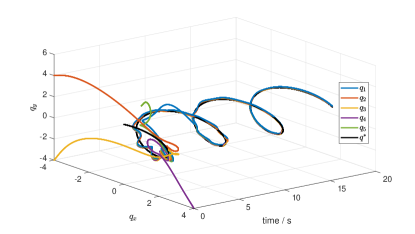
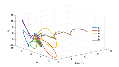
Figure 1: Position trajectories of mobile agents.

Figure 2: Velocity trajectories of mobile agents.

Fig. 2 shows the position trajectories of mobile agents. Fig. 2 shows the velocity trajectories of mobile agents. It can be observed that the positions of all mobile agents ultimately converge to the solution to optimization problem (5).

6 Conclusion

In this paper, time-varying convex optimization problems with uncertain parameters are studied for single-integrator and double-integrator dynamics. By making some common assumptions, we propose a new adaptive algorithm to solve centralized time-varying convex optimization problems. Then, by integrating the new adaptive optimization algorithm and a modified consensus algorithm, the time-varying optimization problems can be solved in a distributed manner. The dependence on Hessian and partial derivative of the gradient with respect to time is reduced through appropriate adaptive law design. These results make it more feasible for multi-agent systems to search the time-varying optimal solution of optimization problems in uncertain high dynamic environments.

Appendix A Proof of Theorem 3

Define a Lyapunov function candidate

$$V= \frac{1}{2}\nabla f_{c}(x,t)^{T}H_{c}^{-1}\nabla f_{c}(x,t)+\frac{1}{2}\zeta^{T}\zeta+\frac{1}{2}tr(\tilde{\eta}_{1}^{T}\gamma_{1}^{-1}\tilde{\eta}_{1})$$

$$+\frac{1}{2}tr(\tilde{\eta}_{2}^{T}\gamma_{2}^{-1}\tilde{\eta}_{2})+\frac{1}{2}tr(\tilde{\eta}_{3}^{T}\gamma_{3}^{-1}\tilde{\eta}_{3}),$$ (46)

where $\tilde{\eta}_{2}=\Omega_{c}-\hat{\eta}_{2}$ and $\tilde{\eta}_{3}=A_{c}-\hat{\eta}_{3}$. Taking the derivative of $V$ along the trajectories of the system (34)-(38) yields

$$\dot{V}= \nabla f_{c}(x,t)^{T}H_{c}^{-1}\frac{d}{dt}{\nabla}f_{c}(x,t)+\zeta^{T}\left(u-\dot{v^{*}}\right)$$

$$+tr(\tilde{\eta}_{1}^{T}\gamma_{1}^{-1}\dot{\tilde{\eta}}_{1})+tr(\tilde{\eta}_{2}^{T}\gamma_{2}^{-1}\dot{\tilde{\eta}}_{2})+tr(\tilde{\eta}_{3}^{T}\gamma_{3}^{-1}\dot{\tilde{\eta}}_{3}).$$ (47)

Note that $\dot{v^{*}}=-\Omega_{c}h_{c}v-A_{c}g_{c}-d/dt\left({h}_{c}^{-1}\hat{\eta}_{1}g_{c}\right)$. Then, we have

$$\dot{V}= \nabla f_{c}(x,t)^{T}v+\nabla f_{c}(x,t)^{T}H_{c}^{-1}\frac{\partial}{\partial{t}}\nabla f_{c}(x,t)$$

$$+\zeta^{T}\left(-{\nabla}f_{c}(x,t)+\tilde{\eta}_{2}h_{c}v+\tilde{\eta}_{3}g_{c}\right)+tr(\tilde{\eta}_{1}^{T}\gamma_{1}^{-1}\dot{\tilde{\eta}}_{1})$$

$$+tr(\tilde{\eta}_{2}^{T}\gamma_{2}^{-1}\dot{\tilde{\eta}}_{2})+tr(\tilde{\eta}_{3}^{T}\gamma_{3}^{-1}\dot{\tilde{\eta}}_{3})$$

$$= -||\nabla f_{c}(x,t)||_{2}^{2}+\nabla f_{c}(x,t)^{T}h_{c}^{-1}\tilde{\eta}_{1}{g}_{c}$$

$$+\zeta^{T}\tilde{\eta}_{2}h_{c}v+\zeta^{T}\tilde{\eta}_{3}g_{c}+tr(\tilde{\eta}_{1}^{T}\gamma_{1}^{-1}\dot{\tilde{\eta}}_{1})$$

$$+tr(\tilde{\eta}_{2}^{T}\gamma_{2}^{-1}\dot{\tilde{\eta}}_{2})+tr(\tilde{\eta}_{3}^{T}\gamma_{3}^{-1}\dot{\tilde{\eta}}_{3})$$

$$= -||\nabla f_{c}(x,t)||_{2}^{2}+tr\left[\tilde{\eta}_{1}^{T}({h_{c}}^{-1})^{T}\nabla f_{c}(x,t){g}_{c}^{T}\right]$$

$$-tr(\tilde{\eta}_{1}^{T}\gamma_{1}^{-1}\dot{\hat{\eta}}_{1})+tr\left(\tilde{\eta}_{2}^{T}\zeta v^{T}h_{c}\right)-tr(\tilde{\eta}_{2}^{T}\gamma_{2}^{-1}\dot{\hat{\eta}}_{2})$$

$$+tr\left(\tilde{\eta}_{3}^{T}\zeta g_{c}^{T}\right)-tr(\tilde{\eta}_{3}^{T}\gamma_{3}^{-1}\dot{\hat{\eta}}_{3})$$

$$= -||\nabla f_{c}(x,t)||_{2}^{2},$$ (48)

where the last equation follows from (36), (37) and (38). Thus, $V(t)\leq V(0)$, $\forall t\geq 0$, which implies the boundedness of $\nabla f_{c}(x,t)$, $\zeta$, $\tilde{\eta}_{1}$, $\tilde{\eta}_{2}$ and $\tilde{\eta}_{3}$. Then, $\hat{\eta}_{1}$, $\hat{\eta}_{2}$ and $\hat{\eta}_{3}$ are bounded. With the definition of $v^{*}$ below (38), $v^{*}$ and $v$ are also bounded. Moreover, $\ddot{V}$ is bounded. By applying Barbalat’s lemma, $\lim_{t\rightarrow\infty}\nabla f_{c}(x,t)=0$. This implies $\lim_{t\rightarrow\infty}(x(t)-x^{*}(t))=0$ by using Lemma 2.

Appendix B Proof of Theorem 4

Step 1: Optimality Analysis

With identicalness of $\Omega_{i}$, define $\Omega_{i}=\Omega$, $\forall i\in\mathcal{N}$. Then, define

$$\tilde{\Omega}=\Omega-\hat{\Omega},~{}~{}~{}~{}~{}\tilde{A}_{i}=A_{i}-\hat{A}_{i},$$ (49)

and $v_{i}^{*}=-\nabla f_{i}(x_{i},t)-{h_{i}}^{-1}\hat{\theta}_{i}g_{i}$, $i\in\mathcal{N}$. Consider the following Lyapunov function candidate

$$V= \frac{1}{2}\zeta_{n}^{T}\left(\sum_{j=1}^{N}H_{j}\right)^{-1}\zeta_{n}+\frac{1}{2}tr\left(\sum_{j=1}^{N}\tilde{\theta}_{j}^{T}\Gamma_{\theta,j}^{-1}\tilde{\theta}_{j}\right)$$

$$+\frac{1}{2}tr\left(\sum_{j=1}^{N}\tilde{A}_{j}^{T}\Gamma_{A,j}^{-1}\tilde{A}_{j}\right)+\frac{1}{2}tr\left(\tilde{\Omega}^{T}\Gamma_{\Omega}^{-1}\tilde{\Omega}\right)$$

$$+\frac{1}{2N}\left(\sum_{j=1}^{N}v_{j}^{*}-\sum_{j=1}^{N}v_{j}\right)^{T}\left(\sum_{j=1}^{N}v_{j}^{*}-\sum_{j=1}^{N}v_{j}\right).$$ (50)

Its derivative along (39)-(44) is given by

$$\dot{V}= \zeta_{n}^{T}\left(\sum_{j=1}^{N}H_{j}\right)^{-1}\left(\sum_{j=1}^{N}H_{j}{v}_{j}+\sum_{j=1}^{N}\frac{\partial}{\partial{t}}\nabla f_{j}(x_{j},t)\right)$$

$$+\frac{1}{N}\left(\sum_{j=1}^{N}v_{j}^{*}-\sum_{j=1}^{N}v_{j}\right)^{T}\left(\sum_{j=1}^{N}\dot{v}_{j}^{*}-\sum_{j=1}^{N}\dot{v}_{j}\right)$$

$$+tr\left(\sum_{j=1}^{N}\tilde{\theta}_{j}^{T}\Gamma_{\theta,j}^{-1}\dot{\tilde{\theta}}_{j}\right)+tr\left(\sum_{j=1}^{N}\tilde{A}_{j}^{T}\Gamma_{A,j}^{-1}\dot{\tilde{A}}_{j}\right)$$

$$+tr\left(\tilde{\Omega}^{T}\Gamma_{\Omega}^{-1}\dot{\tilde{\Omega}}\right)$$ (51)

By using $\sum_{j=1}^{N}\dot{v}_{j}=\sum_{j=1}^{N}\phi_{j}$ and $\dot{v}_{j}^{*}=-\Omega_{j}h_{j}v_{j}-A_{j}g_{j}-d/dt\left({h_{i}}^{-1}\hat{\theta}_{i}g_{i}\right)$, we have

$$\dot{V} =\frac{1}{N}\zeta_{n}^{T}H^{-1}\left(H\sum_{j=1}^{N}v_{j}+\sum_{j=1}^{N}A_{j}g_{j}\right)-\frac{1}{N}\zeta_{g}^{T}$$

$$\times\left(\sum_{j=1}^{N}\nabla f_{j}(x_{j},t)-\tilde{\Omega}\sum_{j=1}^{N}h_{j}{v}_{j}-\sum_{j=1}^{N}\tilde{A}_{j}{g}_{j}\right)$$

$$+tr\left(\sum_{j=1}^{N}\tilde{\theta}_{j}^{T}\Gamma_{\theta,j}^{-1}\dot{\tilde{\theta}}_{j}\right)+tr\left(\sum_{j=1}^{N}\tilde{A}_{j}^{T}\Gamma_{A,j}^{-1}\dot{\tilde{A}}_{j}\right)$$

$$+tr\left(\tilde{\Omega}^{T}\Gamma_{\Omega}^{-1}\dot{\tilde{\Omega}}\right)$$

$$=\frac{1}{N}\zeta_{n}^{T}H^{-1}\sum_{j=1}^{N}A_{j}g_{j}-\frac{1}{N}\left(\zeta_{n}+\sum_{j=1}^{N}h_{j}^{-1}\hat{\theta}_{j}g_{j}\right)^{T}\zeta_{n}$$

$$+\frac{1}{N}\zeta_{g}^{T}\tilde{\Omega}\sum_{j=1}^{N}h_{j}{v}_{j}+\frac{1}{N}\zeta_{g}^{T}\sum_{j=1}^{N}\tilde{A}_{j}{g}_{j}+tr\left(\tilde{\Omega}^{T}\Gamma_{\Omega}^{-1}\dot{\tilde{\Omega}}\right)$$

$$+tr\left(\sum_{j=1}^{N}\tilde{\theta}_{j}^{T}\Gamma_{\theta,j}^{-1}\dot{\tilde{\theta}}_{j}\right)+tr\left(\sum_{j=1}^{N}\tilde{A}_{j}^{T}\Gamma_{A,j}^{-1}\dot{\tilde{A}}_{j}\right).$$ (52)

Recall (22). Then, we have

$$\frac{1}{N}\zeta_{n}^{T}H^{-1}\sum_{j=1}^{N}A_{j}g_{j}-\frac{1}{N}\left(\zeta_{n}+\sum_{j=1}^{N}h_{j}^{-1}\hat{\theta}_{j}g_{j}\right)^{T}\zeta_{n}$$

$$= -\frac{1}{N}||\zeta_{n}||_{2}^{2}+\zeta_{n}^{T}\sum_{j=1}^{N}\left[h_{j}^{-1}\left(\frac{1}{N}\Omega_{j}^{-1}A_{j}-\frac{1}{N}\hat{\theta}_{j}\right)g_{j}\right]$$

$$= -\frac{1}{N}||\zeta_{n}||_{2}^{2}+tr\left[\sum_{j=1}^{N}\tilde{\theta}_{j}^{T}(h_{j}^{-1})^{T}\zeta_{n}g_{j}^{T}\right].$$ (53)

Recall (49). Substitute (B) into (B) yields

$$\dot{V}= -\frac{1}{N}||\zeta_{n}||_{2}^{2}+tr\left[\sum_{j=1}^{N}\tilde{\theta}_{j}^{T}(h_{j}^{-1})^{T}\zeta_{n}g_{j}^{T}\right]$$

$$-\frac{1}{N}tr\left(\sum_{j=1}^{N}\tilde{\theta}_{j}^{T}\Gamma_{\theta,j}^{-1}\dot{\hat{\theta}}_{j}\right)-tr\left(\tilde{\Omega}^{T}\Gamma_{\Omega}^{-1}\dot{\hat{\Omega}}\right)$$

$$+\frac{1}{N}tr\left[\tilde{\Omega}^{T}\zeta_{g}\left(\sum_{j=1}^{N}h_{j}v_{j}\right)^{T}\right]$$

$$+\frac{1}{N}tr\left(\sum_{j=1}^{N}\tilde{A}_{j}^{T}\zeta_{g}g_{j}^{T}\right)-tr\left(\sum_{j=1}^{N}\tilde{A}_{j}^{T}\Gamma_{A,j}^{-1}\dot{\hat{A}}_{j}\right)$$

$$= -\frac{1}{N}||\zeta_{n}||_{2}^{2},$$ (54)

where the last equation follows from (43)-(44). By using the similar analysis below (A), we have $\lim_{t\rightarrow\infty}\zeta_{n}=\lim_{t\rightarrow\infty}\sum_{i=1}^{N}\nabla f_{i}(x_{i},t)=0$. Then, we will give the following consensus analysis to guarantee that the equality constraint in optimization problem (5) holds.

Step 2: Consensus Analysis

System (39) with input (40) can be rewritten as

$$\dot{x}= v,$$

$$\dot{v}= -(L\otimes I_{m})(k_{1}x+k_{2}v)+\phi$$

$$-(DB\otimes I_{m})S[(D^{T}\otimes I_{m})(k_{1}x+k_{2}v)].$$ (55)

According to the definition of $e$ in (28), similarly, define $\delta=(M\otimes I_{m})v$. Then, with the fact that $MD=D$ and $ML=LM=L$, the error system of (B) is

$$\dot{e}= \delta,$$

$$\dot{\delta}= -(L\otimes I_{m})(k_{1}e+k_{2}\delta)+(M\otimes I_{m})\phi$$

$$-(DB\otimes I_{m})S[(D^{T}\otimes I_{m})(k_{1}e+k_{2}\delta)].$$ (56)

Consider the following Lyapunov function candidate

$$W=yPy^{T}+\frac{1}{2}\sum_{i=1}^{N}\sum_{j\in\mathcal{N}_{i}}(\beta_{ij}-\bar{\beta})^{2},~{}~{}y=\operatorname{col}(e,\delta),$$ (57)

where

$$P=\left[\begin{matrix}2k_{1}k_{2}L\otimes I_{m}&k_{1}I_{mN}\\ k_{1}I_{mN}&k_{2}I_{mN}\\ \end{matrix}\right],$$ (58)

and $\bar{\beta}$ is a positive constant to be determined. By using Lemma 1 and Schur Complement Lemma [11], the positive definiteness of $W$ can be guaranteed by choosing $k_{1}$ and $k_{2}$ such that $k_{1}/(2k_{2}^{2})<\lambda_{2}$ with the fact that $e^{T}1_{N}\equiv 0$. Then, the derivative of $W$ along the trajectories of system (B) is given by

$$\dot{W} =-2k_{1}^{2}e^{T}(L\otimes I_{m})e-2\delta^{T}[(k_{2}^{2}L-k_{1}I_{N})\otimes I_{m}]\delta$$

$$-2(k_{1}e+k_{2}\delta)^{T}(DB\otimes I_{m})S[(D^{T}\otimes I_{m})(k_{1}e+k_{2}\delta)]$$

$$+2(k_{1}e+k_{2}\delta)^{T}(M\otimes I_{m})\phi+\sum_{i=1}^{N}\sum_{j\in\mathcal{N}_{i}}(\beta_{ij}-\bar{\beta})\dot{\beta}_{ij}.$$ (59)

From (1), it can be derived that

$$-2(k_{1}e+k_{2}\delta)^{T}(DB\otimes I_{m})S[(D^{T}\otimes I_{m})(k_{1}e+k_{2}\delta)]$$

$$\leq -\sum_{i=1}^{N}\sum_{j\in\mathcal{N}_{i}}\beta_{ij}\left(||k_{1}(e_{i}-e_{j})+k_{2}(\delta_{i}-\delta_{j})||_{1}\right.$$

$$\left.-m\epsilon\exp(-ct)\right).$$ (60)

Note that

$$||\phi_{i}-\phi_{j}||_{2}\leq ||\nabla f_{i}(x_{i},t)-\nabla f_{j}(x_{j},t)||_{2}$$

$$+\hat{\Omega}||h_{i}v_{i}-h_{j}v_{j}||_{2}+||\hat{A}_{i}g_{i}-\hat{A}_{j}g_{j}||_{2}$$

$$+||(d/dt)h_{i}^{-1}\hat{\theta}_{i}{g}_{i}-(d/dt)h_{j}^{-1}\hat{\theta}_{j}{g}_{j}||_{2}.$$ (61)

According to the analysis in Step 1, $\zeta_{n}$, $\hat{\theta}_{i}$, $\hat{\Omega}$ and $\hat{A}_{i}$ are bounded. With the identicalness of $H_{i}(x_{i},t)$ and $\Omega_{i}$, we have $h_{i}=h_{j}$, $\forall i,j\in\mathcal{N}$, $\forall t$. Moreover, $||v_{i}-v_{j}||_{2}$ is also bounded (See [21, Appendix A]). By using Assumption 2, 5 and 7, we know that $g_{i}(x_{i},t)$, $||\nabla f_{i}(x_{i},t)-\nabla f_{j}(x_{j},t)||_{2}$, $(d/dt)g_{i}(x_{i},t)$ and $(d/dt)h_{i}^{-1}(x_{i},t)$ are bounded. Then, there exists a positive constant $\bar{\phi}$ such that $||\phi_{i}-\phi_{j}||_{2}\leq\bar{\phi}$, $\forall i,j\in\mathcal{N}$. By using Assumption 4, we have

$$2(k_{1}e+k_{2}\delta)^{T}(M\otimes I_{m})\phi$$

$$\leq \frac{\bar{\phi}(N-1)}{2}\sum_{i=1}^{N}\sum_{j\in\mathcal{N}_{i}}||k_{1}(e_{i}-e_{j})+k_{2}(\delta_{i}-\delta_{j})||_{1}.$$ (62)

Substituting (B) and (B) into (B) yields

$$\dot{W}\leq -2k_{1}^{2}e^{T}(L\otimes I_{m})e-2\delta^{T}[(k_{2}^{2}L-k_{1}I_{N})\otimes I_{m}]\delta$$

$$-\sum_{i=1}^{N}\sum_{j\in\mathcal{N}_{i}}\beta_{ij}\left(||k_{1}(e_{i}-e_{j})+k_{2}(\delta_{i}-\delta_{j})||_{1}\right.$$

$$\left.-m\epsilon\exp(-ct)\right)+\sum_{i=1}^{N}\sum_{j\in\mathcal{N}_{i}}(\beta_{ij}-\bar{\beta})\dot{\beta}_{ij}$$

$$+\frac{\bar{\phi}(N-1)}{2}\sum_{i=1}^{N}\sum_{j\in\mathcal{N}_{i}}||k_{1}(e_{i}-e_{j})+k_{2}(\delta_{i}-\delta_{j})||_{1}.$$ (63)

Then, by choosing $\bar{\beta}>\bar{\phi}(N-1)/2$, we have

$$\dot{W}\leq -2k_{1}^{2}e^{T}(L\otimes I_{m})e-2\delta^{T}[(k_{2}^{2}L-k_{1}I_{N})\otimes I_{m}]\delta$$

$$+\left(\frac{\bar{\phi}(N-1)}{2}-\bar{\beta}\right)\sum_{i=1}^{N}\sum_{j\in\mathcal{N}_{i}}||k_{1}(e_{i}-e_{j})$$

$$+k_{2}(\delta_{i}-\delta_{j})||_{1}+m\epsilon N^{2}\bar{\beta}\exp(-ct)$$

$$\leq -2k_{1}^{2}\lambda_{2}||e||_{2}^{2}-2(\lambda_{2}k_{2}^{2}-k_{1})||\delta||_{2}^{2}$$

$$+\left(\bar{\phi}(N-1)-2\bar{\beta}\right)\sqrt{\lambda_{2}}||k_{1}e+k_{2}\delta||_{2}$$

$$+m\epsilon N^{2}\bar{\beta}\exp(-ct).$$ (64)

By using the similar analysis below (3), it can be concluded that $e$ and $\delta$ are bounded, and $e,\delta\in\mathcal{L}_{2}$. It follows (B) that $\dot{e}$ and $\dot{\delta}$ are bounded. By applying Barbalat’s lemma, we have $\lim_{t\rightarrow\infty}e(t)=0$ and $\lim_{t\rightarrow\infty}\delta(t)=0$. This further implies $\lim_{t\rightarrow\infty}(x_{i}(t)-x_{j}(t))=0$ and $\lim_{t\rightarrow\infty}(v_{i}(t)-v_{j}(t))=0$, $\forall i,j\in\mathcal{N}$.

Now, combine the analysis in Step 1 and 2. By using Lemma 2, we can conclude that $\lim_{t\rightarrow\infty}(x_{i}(t)-x^{*}(t))=0$, $\forall i\in\mathcal{N}$.

References

• [1] Liwei An and Guang-Hong Yang. Collisions-free distributed optimal coordination for multiple Euler-Lagrangian systems. IEEE Transactions on Automatic Control, 67(1):460–467, 2022.
• [2] Stephen Boyd and Lieven Vandenberghe. Convex Optimization. Cambridge University Press, 2004.
• [3] Lara Briñón-Arranz, Alessandro Renzaglia, and Luca Schenato. Multirobot symmetric formations for gradient and hessian estimation with application to source seeking. IEEE Transactions on Robotics, 35(3):782–789, 2019.
• [4] Fei Chen, Yongcan Cao, and Wei Ren. Distributed average tracking of multiple time-varying reference signals with bounded derivatives. IEEE Transactions on Automatic Control, 57(12):3169–3174, 2012.
• [5] Jorge Cortés and Francesco Bullo. Coordination and geometric optimization via distributed dynamical systems. SIAM Journal on Control and Optimization, 44(5):1543–1574, 2005.
• [6] Zhengtao Ding. Distributed time-varying optimization—an output regulation approach. IEEE Transactions on Cybernetics, 2022. DOI:10.1109/TCYB.2022. 3219295.
• [7] Ruggero Fabbiano, Carlos Canudas De Wit, and Federica Garin. Source localization by gradient estimation based on poisson integral. Automatica, 50(6):1715–1724, June 2014.
• [8] Mahyar Fazlyab, Santiago Paternain, Victor M. Preciado, and Alejandro Ribeiro. Prediction-correction interior-point method for time-varying convex optimization. IEEE Transactions on Automatic Control, 63(7):1973–1986, 2018.
• [9] Bahman Gharesifard and Jorge Cortés. Distributed continuous-time convex optimization on weight-balanced digraphs. IEEE Transactions on Automatic Control, 59(3):781–786, 2013.
• [10] Trevor Halsted, Ola Shorinwa, Javier Yu, and Mac Schwager. A survey of distributed optimization methods for multi-robot systems. arXiv preprint arXiv:2103.12840, 2021.
• [11] Roger A. Horn and Charles R. Johnson. Matrix Analysis. Cambridge University Press, 2nd edition, 2013.
• [12] Bomin Huang, Yao Zou, Ziyang Meng, and Wei Ren. Distributed time-varying convex optimization for a class of nonlinear multiagent systems. IEEE Transactions on Automatic Control, 65(2):801–808, 2020.
• [13] Wanjun Huang, Weiye Zheng, and David J Hill. Distributionally robust optimal power flow in multi-microgrids with decomposition and guaranteed convergence. IEEE Transactions on Smart Grid, 12(1):43–55, January 2021.
• [14] Liangze Jiang, Zhenghong Jin, and Zhengyan Qin. Distributed optimal formation for uncertain euler-lagrange systems with collision avoidance. IEEE Transactions on Circuits and Systems II: Express Briefs, 69(8):3415–3419, 2022.
• [15] Bjorn Johansson, Tamás Keviczky, Mikael Johansson, and Karl Henrik Johansson. Subgradient methods and consensus algorithms for solving convex optimization problems. In 2008 47th IEEE Conference on Decision and Control, pages 4185–4190. IEEE, 2008.
• [16] Björn Johansson, Maben Rabi, and Mikael Johansson. A randomized incremental subgradient method for distributed optimization in networked systems. SIAM Journal on Optimization, 20(3):1157–1170, 2010.
• [17] Hassan K. Khalil. Nonlinear Systems. Prentice Hall, 3rd edition, 2002.
• [18] M. Krstić, I. Kanellakopoulos, and P. V. Kokotović. Nonlinear and Adaptive Control Design. NY: John Wiley & Sons, 1995.
• [19] Tengfei Liu, Zhengyan Qin, Yiguang Hong, and Zhong-Ping Jiang. Distributed optimization of nonlinear multiagent systems: A small-gain approach. IEEE Transactions on Automatic Control, 67(2):676–691, 2022.
• [20] A. Nedic and A. Ozdaglar. Distributed subgradient methods for multi-agent optimization. IEEE Transactions on Automatic Control, 54(1):48–61, 2009.
• [21] Salar Rahili and Wei Ren. Distributed continuous-time convex optimization with time-varying cost functions. IEEE Transactions on Automatic Control, 62(4):1590–1605, 2017.
• [22] S Sundhar Ram, A Nedić, and Venugopal V Veeravalli. Incremental stochastic subgradient algorithms for convex optimization. SIAM Journal on Optimization, 20(2):691–717, 2009.
• [23] Andrea Simonetto, Emiliano Dall’Anese, Santiago Paternain, Geert Leus, and Georgios B. Giannakis. Time-varying convex optimization: Time-structured algorithms and applications. Proceedings of the IEEE, 108(11):2032–2048, 2020.
• [24] Andrea Simonetto, Aryan Mokhtari, Alec Koppel, Geert Leus, and Alejandro Ribeiro. A class of prediction-correction methods for time-varying convex optimization. IEEE Transactions on Signal Processing, 64(17):4576–4591, 2016.
• [25] Wenjing Su. Traffic engineering and time-varying convex optimization. The Pennsylvania State University, 2009.
• [26] Chao Sun, Maojiao Ye, and Guoqiang Hu. Distributed time-varying quadratic optimization for multiple agents under undirected graphs. IEEE Transactions on Automatic Control, 62(7):3687–3694, 2017.
• [27] Yutao Tang, Zhenhua Deng, and Yiguang Hong. Optimal output consensus of high-order multiagent systems with embedded technique. IEEE Transactions on Cybernetics, 49(5):1768–1779, 2019.
• [28] Jing Wang and Nicola Elia. Control approach to distributed optimization. In 2010 48th Annual Allerton Conference on Communication, Control, and Computing (Allerton), pages 557–561. IEEE, 2010.
• [29] Yijing Xie and Zongli Lin. Global optimal consensus for higher-order multi-agent systems with bounded controls. Automatica, 99:301–307, 2019.
• [30] Peng Yi, Yiguang Hong, and Feng Liu. Initialization-free distributed algorithms for optimal resource allocation with feasibility constraints and application to economic dispatch of power systems. Automatica, 74:259–269, 2016.
• [31] Tianpeng Zhang, Victor Qin, Yujie Tang, and Na Li. Source seeking by dynamic source location estimation. In 2021 IEEE/RSJ International Conference on Intelligent Robots and Systems (IROS), pages 2598–2605, 2021.
• [32] Y. Zhang, Y. Lou, Y. Hong, and L. Xie. Distributed projection-based algorithms for source localization in wireless sensor networks. IEEE Transactions on Wireless Communications, 14(6):3131–3142, June 2015.
• [33] Yanqiong Zhang, Zhenhua Deng, and Yiguang Hong. Distributed optimal coordination for multiple heterogeneous Euler–Lagrangian systems. Automatica, 79:207–213, May 2017.
• [34] Yu Zhao, Yongfang Liu, Guanghui Wen, and Guanrong Chen. Distributed optimization for linear multiagent systems: Edge- and node-based adaptive designs. IEEE Transactions on Automatic Control, 62(7):3602–3609, 2017.